Structural Controllability of Switched Continuous and Discrete Time
  Linear Systems

Abstract

This paper explores the structural controllability of switched continuous and discrete time linear systems. It identifies a gap in the proof for a pivotal criterion for structural controllability of switched continuous time systems in the literature. To address this void, we develop novel graph-theoretic concepts, such as multi-layer dynamic graphs, generalized stems/buds, and generalized cactus configurations, and based on them, provide a comprehensive proof for this criterion. Our approach also induces a new, generalized cactus based graph-theoretic criterion for structural controllability. This not only extends Lin’s cactus-based graph-theoretic condition to switched systems for the first time, but also provides a lower bound for the generic dimension of controllable subspaces (which is conjectured to be exact). Finally, we present extensions to reversible switched discrete-time systems, which lead to not only a simplified necessary and sufficient condition for structural controllability, but also the determination of the generic dimension of controllable subspaces.

I Introduction

Switched systems represent a class of hybrid systems where multiple subsystems are regulated by switching laws. This dynamic switching among subsystems can enrich the control strategies, often resulting in superior control performance compared to non-switched systems [1]. For instance, scenarios arise where stabilization through a constant feedback controller remains unattainable, yet becomes feasible through transitions between distinct constant feedback controllers [2]. Due to its significance in both practical applications and theoretical exploration, the study of switched systems has garnered substantial attention [3, 4, 5].

Controllability and observability are two fundamental concepts that are prerequisite for design of switched systems. Extensive investigations have been dedicated to these concepts [3, 6, 4, 7, 8]. Notably, it has been revealed that the reachable and controllable sets of switched continuous-time systems exist as subspaces within the total space, with complete characterizations established in [4]. However, for discrete-time systems, the reachable and controllable sets do not necessarily manifest as subspaces [9]. Geometric characterizations, ensuring these sets to span the entire space, were introduced in [6]. Simplified criteria for reversible systems can be found in [8].

It is important to note that the aforementioned outcomes rely on algebraic computations centered around precise values of system matrices. In practical scenarios, these exact system parameters might be elusive due to modeling inaccuracies or parameter uncertainties [10]. When only the zero-nonzero patterns of system matrices are accessible, Liu et al. [11] introduced the concept of structural controllability for switched systems, aligning with the generic controllability concept initiated by [12]. In [11], several equivalent criteria, grounded in colored union graphs, were proposed to assess structural controllability. Notably, one criterion involves an input accessibility condition and a generic rank condition, distinguished by its simplicity and elegance. This criterion extends naturally from the structural controllability criterion for linear time-invariant (LTI) systems [13]. Exploiting this resemblance, elegant outcomes regarding optimal input selections for LTI systems [14] have been extended to switched systems [15, 16]. Liu et al.’s work has also stimulated research exploration into (strong) structural controllability for other class of time-varying systems, such as linear parameter varying systems [17], temporal networks [18, 19].

Nevertheless, in this paper, we identify a gap in the proof of the criterion’s sufficiency. Regrettably, this gap seems unaddressed if we follow the original research thread in [11] (refer to Section II). Nonetheless, we establish the correctness of the said criterion by providing a rigorous and comprehensive proof for it. Our proof relies on novel graph-theoretic concepts, including multi-layer dynamic graphs, generalized stems, generalized buds, and generalized cactus configurations. Our approach also births a new criterion for structural controllability based on generalized stem-bud structures. Notably, this extends Lin’s cactus-based graph-theoretic condition for structural controllability [20] to switched systems for the first time. This criterion also induces a lower bound for the generic dimension of controllable subspaces, which we conjecture to be exact. Lastly, we extend these results to reversible switched discrete-time systems. This not only yields simplified necessary and sufficient conditions for structural controllability but also enables us to determine the generic dimension of controllable subspaces.

The rest are organized as follows. Section II provides some basic preliminaries and the motivation of this paper by identifying a gap in the existing literature. Section III presents a new generalized cactus configuration based criterion for structural controllability and establishes the correctness of the existing one. Extensions to reversible switched discrete-time systems are given in Section IV. The last section concludes this paper.

II Preliminaries and Motivation

II-A Controllability of switched systems

Consider a switched continuous time linear system whose dynamics is governed by [5]

$$\dot{x}(t)=A_{\sigma(t)}x(t)+B_{\sigma(t)}u_{\sigma(t)}(t),$$ (1)

where $x(t)\in{\mathbb{R}}^{n}$ is the state, $\sigma(t):[0,\infty)\to\{1,...,N\}$ is the switching signal that can be designed, $u_{\sigma(t)}(t)\in{\mathbb{R}}^{m_{\sigma(t)}}$ is the piecewise continuous input, $m_{i}\in{\mathbb{N}}$, $i=1,...,N$. $(A_{i},B_{i})$ is called a subsystem of system (1), $i=1,...,N$. $\sigma(t)=i$ implies the subsystem $(A_{i},B_{i})$ is activated as the system realization at time instant $t$. We may use the matrix set $(A_{i},B_{i})|_{i=1}^{N}$ to denote the switched system (1).

Definition 1 ([4])

A state $x\in{\mathbb{R}}^{n}$ is said to be controllable, if there exists a finite $t_{f}$, a switching signal $\sigma(t):[0,t_{f})\to\{1,...,N\}$ and an input $u(t)\in{\mathbb{R}}^{m_{\sigma(t)}}$, $t\in[0,t_{f})$, such that $x(0)=x$ and $x(t_{f})=0$. The controllable set (controllable subspace) of system (1) is the set of controllable states. System (1) is said to be controllable, if its controllable set is ${\mathbb{R}}^{n}$.

It is noted that if we change ‘$x(0)=x$ and $x(t_{f})=0$’ to ‘$x(0)=0$ and $x(t_{f})=x$’ in Definition 1, then the concept ‘reachability’ can be defined. For switched continuous time systems and reversible switched discrete time systems (see Section IV), their reachability and controllability always coincide [4, 6].

Lemma 1 ([4])

The switched system (1) is controllable, if and only if the following controllability matrix ${\cal R}$ has full row rank:

$${\cal R}=\left[A_{i_{n}}^{j_{n}}A_{i_{n-1}}^{j_{n-1}}\cdots A_{i_{1}}^{j_{1}}B_{i_{1}}|_{i_{1},...,i_{n}=1,...,N}^{j_{n},...,j_{1}=0,...,n-1}\right].$$

Here, each item $A_{i_{n}}^{j_{n}}\cdots A_{i_{1}}^{j_{1}}B_{i_{1}}$ constitutes sub-columns of ${\cal R}$. Moreover, the controllable subspace of system (1) is the column space spanned by ${\cal R}$, denoted as ${\rm span}{\cal R}$, and its dimension equals ${\rm rank}{\cal R}$.

A structured matrix is a matrix with either fixed zero entries or free entries that can take values independently (the latter are called nonzero entries). The generic rank of a structured matrix (or a polynomial of structured matrices), given by ${\rm grank}$, is the maximum rank it can achieve as a function of parameters for its nonzero entries. It turns out that the generic rank is also the rank this matrix can achieve for almost all values of its nonzero entries. When only the zero-nonzero patterns of matrices $(A_{i},B_{i})|_{i=1}^{N}$ are available, that is, $(A_{i},B_{i})|_{i=1}^{N}$ are structured matrices, system (1) is called a structured system. $(\tilde{A}_{i},\tilde{B}_{i})|_{i=1}^{N}$ is a realization of $(A_{i},B_{i})|_{i=1}^{N}$, if $\tilde{A}_{i}$ ($\tilde{B}_{i}$) is obtained by assigning some particular values to the nonzero entries of $A_{i}$ ($\tilde{B}_{i}$), $i=1,...,N$.

Definition 2 ([11])

A structured system (1) is said to be structurally controllable, if there is a realization $(\tilde{A}_{i},\tilde{B}_{i})|_{i=1}^{N}$ of $(A_{i},B_{i})|_{i=1}^{N}$, such that $(\tilde{A}_{i},\tilde{B}_{i})|_{i=1}^{N}$ is controllable.

From Lemma 1, if a (structured) system is structurally controllable, then almost all its realizations are controllable. This generic property makes the concept appealing, particularly for large-scale network systems [10].

II-B Graph-theoretic preliminaries

A directed graph (digraph) is denoted by ${\cal G}=(V,E)$, where $V$ is the vertex set, and $E\subseteq V\times V$ is the edge set. A subgraph of ${\cal G}$ is a graph ${\cal G}_{s}=(V_{s},E_{s})$ such that $V_{s}\subseteq V$ and $E_{s}\subseteq E$, and is called a subgraph induced by $V_{s}$, if $E_{s}=(V_{s}\times V_{s})\cap E$. We say ${\cal G}_{s}$ covers $V_{s}^{\prime}\subseteq V$ if $V_{s}^{\prime}\subseteq V_{s}$, and ${\cal G}_{s}$ spans ${\cal G}$ if $V_{s}=V$. An edge from $i_{1}$ to $i_{2}$, given by $(i_{1},i_{2})$, is called an ingoing edge of vertex $i_{2}$, and an outgoing edge of vertex $i_{1}$. A sequence of successive edges $(i_{1},i_{2}),(i_{2},i_{3}),...,(i_{k-1},i_{k})$ is called a walk from vertex $i_{1}$ to vertex $i_{k}$. Such a walk $p$ is either denoted by the sequence of edges it contains, i.e., $p=(e_{1},e_{2},...,e_{k-1})$, where $e_{j}=(i_{j},i_{j+1})$, or the sequence of vertices it passes, i.e., $p=(i_{1},i_{2},...,i_{k})$. Vertex $i_{1}$ is called the tail (initial vertex), denoted as ${\rm tail}(p)$, and vertex $i_{k}$ is called the head (terminal vertex), denoted as ${\rm head}(p)$. The length of a walk $p$, given by $|p|$, is the edges it contains (counting repeated edges). A walk without repeated vertices is called a path. A walk from a vertex to itself is called a loop. If the head (or tail) of a loop is the only repeated vertex when traversing along its way, this loop is called a cycle.

Two typical graph-theoretic presentations of system (1) are introduced. For the $i$th subsystem, the system digraph ${\cal G}_{i}=(V_{Xi}\cup V_{Ui},E_{XXi}\cup E_{UXi})$, where the state vertices $V_{Xi}=\{v^{i}_{1},...,v^{i}_{n}\}$, the input vertices $V_{Ui}=\{v^{i}_{n+1},...,v^{i}_{n+m_{i}}\}$, the state edges $E_{XXi}=\{(v^{i}_{k},v^{i}_{j}):A_{i,jk}\neq 0\}$, and input edges $E_{UXi}=\{(v^{i}_{n+k},v^{i}_{j}):B_{i,jk}\neq 0\}$. The colored union graph ${\cal G}_{c}$ of system (1) is the union of ${\cal G}_{1},\cdots,{\cal G}_{N}$ by using different colors to distinguish state edges from different subsystems. More precisely, ${\cal G}_{c}$ is a digraph ${\cal G}_{c}=(X\cup U,E_{XX}\cup E_{UX})$, where $X=\{v_{1},...,v_{n}\}$, $U=V_{U1}\cup\cdots\cup V_{UN}$, $E_{XX}=\{(v_{k},v_{j}):A_{i,jk}\neq 0,i=1,...,N\}$, and $E_{UX}=\{(v^{i}_{n+k},v_{j}):B_{i,jk}\neq 0,i=1,...,N,k=1,...,m_{i}\}$. Notice that multiple edges are allowable in $E_{XX}$, and to distinguish them, we assign the color index $i$ to the edge $(v_{k},v_{j})$ (resp. $(v_{n+k},v_{j})$) corresponding to $A_{i,jk}\neq 0$ ($B_{i,jk}\neq 0$), $i\in\{1,...,N\}$. An edge $(v_{k},v_{j})$ with color index $i$ is also denoted by $e_{kj}^{i}$. A stem is a path from some $u\in U$ to some $v\in X$ in ${\cal G}_{c}$.

Definition 3

A state vertex $v_{i}\in X$ is said to be input-reachable, if there is a path from an input vertex $u\in U$ to $v$ in ${\cal G}_{c}$.

Definition 4 ([11])

In the colored union graph ${\cal G}_{c}$, $k$ edges are said to be S-disjoint if their heads are all distinct and if all the edges that have the same tail have different color indices.

The following lemma reveals the relation between the $S$-disjoint edge and ${\rm grank}[A_{1},...,A_{N},B_{1},...,B_{N}]$.

Lemma 2 ([11])

There are $n$ $S$-disjoint edges in ${\cal G}_{c}$, if and only if ${\rm grank}[A_{1},...,A_{N},B_{1},...,B_{N}]=n$.

II-C Motivation of this paper

Liu et al. [11] propose a criterion for the structural controllability of system (1). This criterion says system (1) is structurally controllable, if and only if two conditions hold: (i) every state vertex is input-reachale in ${\cal G}_{c}$, and (ii) ${\rm grank}[A_{1},...,A_{N},B_{1},...,B_{N}]=n$ (see [11, Theo 9]).

The necessity of conditions (i) and (ii) is relatively straightforward. The sufficiency, however, is not. In the proof for the sufficiency of conditions (i) and (ii), the authors of [11] intended to show that if the switched system (1) is not structurally controllable and condition (i) holds, then condition (ii) cannot hold, i.e., ${\rm grank}[A_{1},...,A_{N},B_{1},...,B_{N}]<n$. To achieve this, the authors argued that if for every matrix pair $(\tilde{\bar{A}},\tilde{\bar{B}})$, where $\tilde{\bar{A}}=\sum\nolimits_{i=1}^{N}\bar{u}_{i}\bar{A}_{i}$, $\tilde{\bar{B}}=\sum\nolimits_{i=1}^{m}\bar{u}_{i}\bar{B}_{i}$, $(\bar{A}_{i},\bar{B}_{i})$ can be any realization of $(A_{i},B_{i})$, and $\bar{u}_{1},...,\bar{u}_{N}\in{\mathbb{R}}$, there is a nonzero vector $q$ such that $q\tilde{\bar{A}}=0$ and $q\tilde{\bar{B}}=0$, then ${\rm grank}[A_{1},...,A_{m},B_{1},...,B_{m}]=n$ cannot hold. However, this claim is not necessarily true. The following counter-example demonstrates this.

Example 1

Consider a switched system with $N=2$, whose subsystem parameters are ($a_{21},a_{31},b_{1}\in{\mathbb{R}}$):

$$A_{1}=\left[\begin{array}[]{ccc}0&0&0\\ a_{21}&0&0\\ 0&0&0\\ \end{array}\right],B_{1}=\left[\begin{array}[]{c}b_{1}\\ 0\\ 0\end{array}\right],$$

$$A_{2}=\left[\begin{array}[]{ccc}0&0&0\\ 0&0&0\\ a_{31}&0&0\\ \end{array}\right],B_{2}=\left[\begin{array}[]{c}0\\ 0\\ 0\end{array}\right].$$

Then, ${\rm grank}[A_{1},A_{2},B_{1},B_{2}]=3$. However, for $\bar{u}_{1},\bar{u}_{2}\in{\mathbb{R}}$,

$$[\bar{u}_{1}A_{1}+\bar{u}_{2}A_{2},\bar{u}_{1}B_{1}+\bar{u}_{2}B_{2}]=\left[\begin{array}[]{cccc}0&0&0&\bar{u}_{1}b_{1}\\ \bar{u}_{1}a_{21}&0&0&0\\ \bar{u}_{2}a_{31}&0&0&0\\ \end{array}\right].$$

It follows that for all the values of $a_{21},a_{31},b_{1}$ and $\bar{u}_{1},\bar{u}_{2}$, ${\rm rank}[\bar{u}_{1}A_{1}+\bar{u}_{2}A_{2},\bar{u}_{1}B_{1}+\bar{u}_{2}B_{2}]<3$. Hence, there exists a corresponding nonzero vector $q$, such that $q[\bar{u}_{1}A_{1}+\bar{u}_{2}A_{2},\bar{u}_{1}B_{1}+\bar{u}_{2}B_{2}]=0$.

In fact, the essential idea of the above-mentioned proof in [11] is to derive the structural uncontrollability of the switched system $(A_{i},B_{i})|_{i=1}^{N}$ from the structural uncontrollability of the LTI system $(\tilde{\bar{A}},\tilde{\bar{B}})$. However, this direction is not necessarily true, since the structural controllability of $(A_{i},B_{i})|_{i=1}^{N}$ does not imply the structural controllability of $(\tilde{\bar{A}},\tilde{\bar{B}})$. The primary goal of this paper is to develop new criteria for structural controllability of switched systems, and meanwhile, rigorously establish the sufficiency (and necessity) of conditions (i) and (ii),

III Generalized cactus configuration and structural controllability

This section presents a novel generalized stem-bud based criterion for the structural controllability of switched systems. Based on it, the sufficiency of conditions (i) and (ii) is established. Key to this new criterion is the introduction of some novel graph-theoretic concepts, detailed in the first two subsections.

III-A Multi-layer dynamic graph

Given a subspace ${\cal V}\subseteq{\mathbb{R}}^{n}$, let $\Gamma_{A}{\cal V}=\sum_{i=0}^{n-1}A^{i}{\cal V}$. Let $\left\langle A|B\right\rangle=\sum_{i=0}^{n-1}A^{i}{\rm Im}B$ be the controllable subspace of $(A,B)$, with ${\rm Im}B$ being the subspace spanned by the columns of $B$. From [4], the controllable subspace of system (1), denoted by $\bf\Omega$, can be iteratively expressed as

$${\mathbf{\Omega}}_{1}=\sum_{i=1}^{N}\langle A_{i}|B_{i}\rangle,\ {\mathbf{\Omega}}_{i}=\sum_{k=1}^{N}\Gamma_{A_{k}}{\bf\Omega}_{i-1},i=2,...,n.$$

Then, ${\mathbf{\Omega}}={\rm span}{\cal R}={\mathbf{\Omega}}_{n}$.

Inspired by [4], we define the nested subspaces $\{{\bf\Phi}_{i}|_{i=0}^{\infty}\}$ as

$$\begin{array}[]{c}{\bf\Phi}_{0}={\rm Im}\ B_{1}+{\rm Im}\ B_{2}+\cdots+{\rm Im}\ B_{N},\\ {\bf\Phi}_{j}=\sum\nolimits_{i=1}^{N}A_{i}{\bf\Phi}_{j-1},j=1,....\infty\end{array}$$

Construct $\{{\bf W}_{j}|_{j=-1}^{\infty}\}$ as ${\bf W}_{-1}=\emptyset$, ${\bf W}_{j}={\bf W}_{j-1}+{\bf\Phi}_{j}$ for $j=0,1,\cdots,\infty$. This implies ${\bf W}_{j}=\sum_{i=0}^{j}{\bf\Phi}_{i}$ ($j=0,1,\cdots,\infty$), ${\bf W}_{0}\subseteq{\bf W}_{1}\subseteq\cdots\subseteq{\bf W}_{\infty}$, and ${\bf W}_{\infty}={\bf\Omega}$. It turns out that ${\bf W}_{j}={\bf W}_{j-1}+\sum\nolimits_{i=1}^{N}A_{i}{\bf W}_{j-1}$. Therefore, if for some $j$, it holds ${\bf W}_{j}={\bf W}_{j+1}$, then ${\bf W}_{j+2}={\bf W}_{j+1}+\sum\nolimits_{i=1}^{N}A_{i}{\bf W}_{j+1}={\bf W}_{j}+\sum\nolimits_{i=1}^{N}A_{i}{\bf W}_{j}={\bf W}_{j+1}$, leading to ${\bf W}_{k}={\bf W}_{j}={\bf\Omega}$ for any $k\geq j$. This means there exists some $l_{0}\leq n$, such that ${\bf W}_{\bar{l}}={\bf\Omega}$ for any $\bar{l}\geq l_{0}$. It is worth noting that the difference between the nested subspaces $\{{\bf\Phi}_{j}|_{j=0}^{\infty}\}$ and those in [4, Sec 4.3] lies in that, ${\bf\Phi}_{j}$ does not necessarily contain ${\bf\Phi}_{j-1}$, which is important to reduce the redundant edges in constructing the associated dynamic graphs shown below.

Corresponding to $\{{\bf\Phi}_{i}|_{i=0}^{\infty}\}$, define the matrix series $\{\Gamma_{j}|_{j=0}^{\infty}\}$ as

$$\Gamma_{0}=[B_{1},...,B_{N}],$$

$$\Gamma_{j}=[A_{i}\Gamma_{j-1}|_{i=1}^{N}],j=1,2...$$

Moreover, let

$$W_{0}=\Gamma_{0},W_{j}=[W_{j-1},\Gamma_{j}],j=1,...\infty$$

Following the above analysis, if ${\rm rank}W_{j}={\rm rank}W_{j+1}$ for some $j$, then ${\rm rank}W_{k}={\rm rank}W_{j}$ for any $k\geq j$. Since all the above relations hold for any numerical matrices, they must hold when ‘${\rm rank}$’ is replaced by ‘${\rm grank}$’ (the corresponding matrices $(A_{i},B_{i})$ become structured ones).

In what follows, we construct the dynamic graphs $\{\hat{\cal G}_{i}:i=0,1,\cdots,\bar{l}\}$ associated with $\{W_{i}|_{i=0}^{\bar{l}}\}$ iteratively, with $\bar{l}\geq l_{0}\doteq n-{\rm grank}\Gamma_{0}$. In the construction, we shall use the state vertex notation $v_{\#\circ}^{\star\bullet}$, in which superscripts $\star$, $\bullet$ denote the subsystem and copy indices, while subscripts $\#,\circ$ indicates its index in $X$ and the layer index, respectively, and so is the input vertex notation $v_{\#,t\circ}^{\star\bullet}$, in which the extra ‘$t$’ indicates which subsystem this input vertex is copied from (‘layer’ and ‘copy’ shall be explained subsequently). At the beginning, ${\hat{\cal G}}_{0}=(\hat{V}_{0},\hat{E}_{0})$ with $\hat{V}_{0}=\hat{V}_{U0}\cup\hat{V}_{X0}$, $\hat{V}_{X0}=\{v_{j0}^{00}:j=1,...,n\}$, $\hat{V}_{U0}=\{v_{n+k,j0}^{00}:j=1,...,N,k=1,...,m_{j}\}$, and $\hat{E}_{0}=\{(v_{n+k,j0}^{00},v_{q0}^{00}):B_{j,qk}\neq 0,j=1,...,N,k=1,...,m_{j}\}$. For $i\geq 1$, ${\hat{\cal G}}_{i}$ is obtained by adding vertices $\hat{V}_{i}=\hat{V}_{Ui}\cup\hat{V}_{Xi}$ and the associated edges $\hat{E}_{i}\cup\hat{E}_{i,i-1}$ to $\hat{\cal G}_{i-1}$, where $\hat{V}_{Xi}=\{v_{ji}^{kt}:j=1,...,n,k=1,...,N,t=1,...,N^{i-1}\}$, $\hat{V}_{Ui}=\{v^{kt}_{n+j,li}:k,l=1,...,N,j=1,...,m_{l},t=1,...,N^{i-1}\}$, and $\hat{E}_{i}=\{(v^{pl}_{n+k,ti},v^{pl}_{qi}):p,t=1,...,N,l=1,...,N^{i-1},k=1,...,m_{t},B_{t,qk}\neq 0\}$. The edge set $\hat{E}_{i,i-1}$ is defined as

$$\hat{E}_{i,i-1}=\bigcup_{{\tiny{\begin{array}[]{c}k=1,...,N,\\ A_{k,pj}\neq 0\end{array}}}}\begin{array}[]{c}\left\{(v_{ji}^{k1},v_{p,i-1}^{11}),(v_{ji}^{k2},v_{p,i-1}^{12}),\right.\\ \left.\cdots,(v_{ji}^{kN^{i-1}},v_{p,i-1}^{NN^{i-2}})\right\},\end{array}$$

that is, for each $k\in\{1,...,N\}$, there is exactly one edge from the $t$th vertex of $\{v^{k1}_{ji},\cdots,v^{kN^{i-1}}_{ji}\}$ to the $t$th vertex of $\hat{V}_{X,i-1}=\{v_{p,i-1}^{11},v_{p,i-1}^{12},\cdots,v_{p,i-1}^{1N^{i-2}},\cdots,v_{p,i-1}^{NN^{i-2}}\}$ whenever $A_{k,pj}\neq 0$, for $t=1,...,N^{i-1}$, where we set $N^{-1}=0$, and $v^{q0}_{p,0}\equiv v^{00}_{p0}$ for $q=1,...,N$ and multiple edges are disallowed (i.e., $\hat{E}_{1,0}=\{(v_{j1}^{k1},v^{00}_{p0}):k=1,...,N,A_{k,pj}\neq 0\}$). For an edge $e=(v_{ji}^{ks},v_{p,i-1}^{k^{\prime}s^{\prime}})\in\hat{E}_{i,i-1}$, the weight $w(e)=A_{k,pj}$, and for an edge $e=(v_{n+k,ti}^{pl},v_{qi}^{pl})\in\hat{E}_{i}$, its weight $w(e)=B_{t,qk}$.

We call the subgraph of ${\hat{\cal G}}_{\bar{l}}$ induced by $\hat{V}_{i}$ the $i$th layer, $i=0,...,\bar{l}$. As can be seen, in the $i$th layer ($i\geq 1$), we copy the state vertex set $\{v^{j}_{1},...,v^{j}_{n}\}$ of the $j$th subsystem $N^{i-1}$ times (thus each set is called a copy), and each copy of them is connected to a copy of input vertices of the $1,...,N$-th subsystems. Moreover, between two successive layers, there are edges (corresponding to nonzero entries of $A_{k}$) from each copy of state vertices ($N^{i-1}$ copies in total) of the $k$th subsystem in $i$th layer to one and only one copy of state vertices of the $1,2,...,N$th subsystems in the $(i-1)$th layer, $k=1,...,N$, $i=1,...,\bar{l}$. Since $\hat{\cal G}_{\bar{l}}$ has multiple layers, we call it the multi-layer dynamic graph (MDG). See Fig. 1 for illustration of an MDG associated with a switched system. It can be seen that MDG generalizes the dynamic graph adopted in [21] for LTI systems to switched systems.

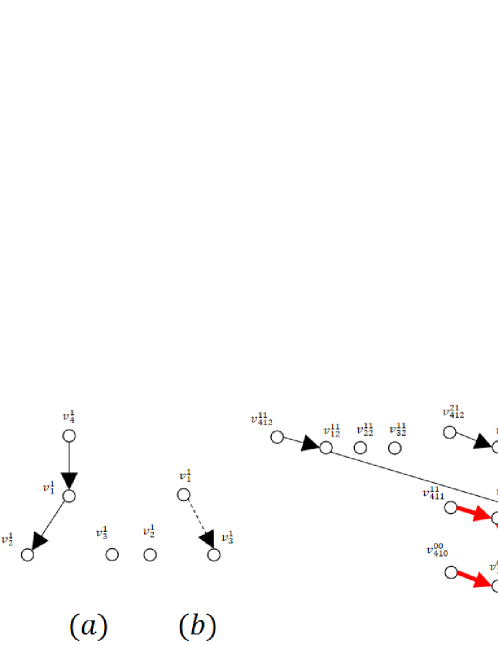
Figure 1: Illustration of MDG of a switched system with two subsystems, where (a) and (b) are respectively the subsystem digraphs ${\cal G}_{1}$ and ${\cal G}_{2}$, and (c) is the MDG $\hat{\cal G}_{2}$ with $3$ layers. Throughout this paper, edges with different color indices are depicted with different styles of lines. Bold red lines represent a $\hat{V}_{U}-\hat{V}_{X0}$ linking with size $3$.

A collection of $k$ vertex-disjoint paths $L=(p_{1},...,p_{k})$ in $\hat{\cal G}_{\bar{l}}$ is called a linking (with size $k$). We call $L$ a $S-T$ linking, if ${\rm tail}(L)\doteq\{{\rm tail}(p_{i}):i=1,...,k\}\subseteq S$, and ${\rm head}(L)\doteq\{{\rm head}(p_{i}):i=1,...,k\}\subseteq T$. We are interested in the linkings from $\hat{V}_{U}$ to $\hat{V}_{X0}$, where $\hat{V}_{U}=\bigcup_{i=0}^{\bar{l}}\hat{V}_{Ui}$ (the dependence of $\bar{V}_{U}$ on $\bar{l}$ is omitted for simplification), i.e., $S-T$ linkings with $S\subseteq\hat{V}_{U}$ and $T\subseteq\hat{V}_{X0}$. For such a linking $L=(p_{1},...,p_{k})$, define $w(p_{i})$ as the product of weights of all individual edges in each path $p_{i}$ of $L$, $i=1,...,k$, and $w(L)=w(p_{1})w(p_{2})\cdots w(p_{k})$. Let $\prec$ be a fixed order of vertices in $\hat{V}_{U}$ and $\hat{V}_{X0}$. For a linking $L=(p_{1},...,p_{k})$, let $s_{1}\prec s_{2}\prec\cdots\prec s_{k}$ and $t_{1}\prec t_{2}\prec\cdots\prec t_{k}$ be respectively the tails and heads of $L$. Moreover, suppose $s_{\pi{(i)}}$ and $t_{i}$ are the tail and head of the path $p_{i}$, $i=1,...,k$. Then, we obtain a permutation $\pi\doteq(\pi(1),...,\pi(k))$ of $(1,2,...,k)$, and denote its sign by ${\rm sign}(\pi)\in\{1,-1\}$. Recall that the sign of a permutation is defined as $(-1)^{q}$, where $q$ is the number of transpositions required to transform the permutation into an ordered sequence.

Let $A_{i}(j,p)$ be the $(j,p)$th entry of $A_{i}$, and $B_{i}(j,p)$ defined similarly. Observe that the $(t_{k},t_{0}^{\prime})$th entry of $A_{i_{k}}A_{i_{k-1}}\cdots A_{i_{1}}B_{i_{0}}$ is the sum of all products in the form of

$$A_{i_{k}}(t_{k},t_{k-1})A_{i_{k-1}}(t_{k-1},t_{k-2})\cdots A_{i_{1}}(t_{1},t_{0})B_{i_{0}}(t_{0},t_{0}^{\prime}),$$ (2)

where $k\leq\bar{l}$, $t_{k},t_{k-1},...,t_{0}=1,...,n$, $i_{k},...,i_{0}=1,...,N$, and each involved entry in the product is nonzero. We call such a nonzero term a product term in $W_{\bar{l}}$. By the construction of $\hat{\cal G}_{\bar{l}}$, for each product term (2), there exists a path

$$p\doteq(v_{n+t_{0}^{\prime},i_{0}k}^{i_{1},j_{1}},v^{i_{1},j_{1}}_{t_{0},k},v_{t_{1},k-1}^{i_{2},j_{2}},\cdots,v_{t_{k-1},1}^{i_{k},j_{k}},v^{00}_{t_{k},0})$$ (3)

with head in $\hat{V}_{X0}$ and tail in $\hat{V}_{U}$ of $\hat{\cal G}_{\bar{l}}$, where $j_{1},...,j_{k}$ are the corresponding copy indices in the $k$th,$\cdots,1$st layers, respectively; and vice versa, that is, any $\hat{V}_{U}-\hat{V}_{X0}$ path, say $p$, corresponds to a unique product term in ${\cal W}_{l}$.

Denote by $W_{\bar{l}}(I,J)$ the submatrix of $W_{\bar{l}}$ given by rows corresponding to $I$ and columns corresponding to $J$. Based on the above relation, there are one-one correspondences between rows of $W_{\bar{l}}$ and the set $\hat{V}_{X0}$, and between columns of $W_{\bar{l}}$ and the set $\hat{V}_{U}$. The following proposition relates the determinant of a square sub-matrix $W_{\bar{l}}(I,J)$ to the $J-I$ linkings of $\hat{\cal G}_{\bar{l}}$.

Proposition 1

Let $W_{\bar{l}}(I,J)$ be a square-sub matrix of $W_{\bar{l}}$. Then

$$\det W_{\bar{l}}(I,J)=\sum_{L:\ J-I\ {\rm linking\ with\ size}\ |I|\ {\rm in}\ \hat{\cal G}_{\bar{l}}}{\rm sign}(L)w(L),$$ (4)

where $J$ and $I$ are regarded as subsets of $\hat{V}_{U}$ and $\hat{V}_{X0}$, respectively.

Proof:

Based on the above analysis, the entry at the position $(v_{t_{k},0}^{00},v_{n+t_{0}^{\prime},t_{0}k}^{i_{0},j_{1}})$ of $W_{\bar{l}}$, with $v_{t_{k},0}^{00}\in\hat{V}_{X0}$, $v_{n+t_{0}^{\prime},t_{0}k}^{i_{0},j_{1}}\in\hat{V}_{U}$, is expressed as

$$W_{\bar{l}}(v_{t_{k},0}^{00},v_{n+t_{0}^{\prime},t_{0}k}^{i_{0},j_{1}})=\sum_{p}w(p),$$ (5)

where the summation is taken over all paths $p$ in $\hat{\cal G}_{\bar{l}}$ from $v_{n+t_{0}^{\prime},t_{0}k}^{i_{0},j_{1}}$ to $v_{t_{k},0}^{00}$, i.e., all paths in the form of (3). With the understanding of $J\subseteq\hat{V}_{U}$ and $I\subseteq\hat{V}_{X0}$, by submitting (5) into the expression of the determinant, we have

$$\det W_{\bar{l}}(I,J)=\sum_{\pi}{\rm sign}(\pi)\prod_{v_{t_{k},0}^{00}\in I}W_{\bar{l}}(v_{t_{k},0}^{00},\pi(v_{t_{k},0}^{00})),$$ (6)

where the summation is taken over all permatations $\pi:I\to J$ such that $\prod\nolimits_{v_{t_{k},0}^{00}\in I}W_{\bar{l}}(v_{t_{k},0}^{00},\pi(v_{t_{k},0}^{00}))\neq 0$.

Notice that each nonzero $\prod\nolimits_{v_{t_{k},0}^{00}\in I}W_{\bar{l}}(v_{t_{k},0}^{00},\pi(v_{t_{k},0}^{00}))$ is the product of weights of $|I|$ paths, each path from $\pi(i)\in J$ to $i\in I$, given by $p_{\pi(i),i}$. Let $P_{\pi}$ be the collection of such $|I|$ paths. If two paths $p_{\pi(i),i},p_{\pi(i^{\prime}),i^{\prime}}\in P_{\pi}$ intersect at a vertex $v$, let $w$ and $\sigma$ be respectively the path from $\pi(i)$ to $v$ and the path from $v$ to $i$ in $p_{\pi(i),i}$, and $w^{\prime}$ and $\sigma^{\prime}$ be the path from $\pi(i^{\prime})$ to $v$ and the path from $v$ to $i^{\prime}$ in $p_{\pi(i^{\prime}),i^{\prime}}$. Then, two new paths are constructed by connecting $w$ with $\sigma^{\prime}$ and $w^{\prime}$ with $\sigma$, and the remaining paths remain unchanged. This produces a new collection of $|I|$ paths, denoted by $P_{\pi^{\prime}}$, with $\pi^{\prime}(i)=\pi(i^{\prime})$ and $\pi^{\prime}(i^{\prime})=\pi(i)$, leading to ${\rm sign}(\pi^{\prime})=-{\rm sign}(\pi)$, while $\prod\nolimits_{p_{i}\in P_{\pi}}w(p_{i})=\prod\nolimits_{p_{i}\in P_{\pi^{\prime}}}w(p_{i})$. It is easy to see the correspondence between such $P_{\pi}$ and $P_{\pi^{\prime}}$ is one-to-one in all $|I|$ paths from $J$ to $I$. Consequently, all collections of $|I|$ paths from $J$ to $I$ that are not vertex-disjoint will cancel out in (6). This leads to (4). ∎

Remark 1

A direct corollary of Proposition 1 is that the generic dimension of controllable subspaces ${\rm grank}{\cal R}$ is no more than the maximum size of a $\hat{V}_{U}-\hat{V}_{X0}$ linking in $\hat{\cal G}_{\bar{l}}$, $\bar{l}\geq l_{0}$.

III-B Generalized stem, bud, and cactus walking/configuration

Now we introduce some new graph-theoretic notions, namely, generalized stem, generalized bud, generalized cactus configuration, and generalized cactus walking, which extends the corresponding graph-theoretic concepts from LTI systems to switched systems. These extensions are crucial to our results.

Definition 5 (Generalized stem)

A subgraph ${\cal G}_{s}\!=\!(V_{s},E_{s})$ of the color union graph ${\cal G}_{c}$ is said to be a generalized stem, if ${\cal G}_{s}$ satisfies:

• There is only one input vertex $u\in V_{s}$ and no cycle;

• Each state vertex $x\in V_{s}\backslash\{u\}$ has exactly one ingoing edge (thus $|E_{s}|=|V_{s}|-1$);

• All edges of $E_{s}$ are S-disjoint.

Definition 6 (Generalized bud)

A subgraph ${\cal G}_{s}=(V_{s},E_{s})$ of the color union graph ${\cal G}_{c}$ is said to be a generalized bud, if ${\cal G}_{s}$ satisfies:

• There is no input vertex in $V_{s}$ and only one cycle;

• Every state vertex $x\in V_{s}$ is input-reachable in ${\cal G}_{c}$;

• Each state vertex $x\in V_{s}$ has exactly one ingoing edge (thus $|E_{s}|=|V_{s}|$);

• All edges of $E_{s}$ are S-disjoint.

Fig. 2 presents an example of a generalized stem and a generalized bud. It can be verified that when ${\cal G}_{c}$ is the system digraph of an LTI system (i.e., without being colored), the generalized stem collapses to a conventional stem, and the generalized bud collapses to a cycle which is input-reachable.

Definition 7

A subset $X_{s}\subset X$ is said to be covered by a generalized cactus configuration, if there is a collection of vertex-disjoint generalised stems and generalised buds that cover $X_{s}$.

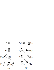
Figure 2: Example of a generalized stem (a) and generalized bud (b). In (a), ‘u’ represents an input vertex. Note that there are $3$ different color indices, depicted by $3$ different line styles.

Before introducing the notion generalized cactus walking, some notations on walks of the colored union graph ${\cal G}_{c}$ are presented. Given a walk $p=(e^{i_{1}}_{j_{1},j_{2}},e^{i_{2}}_{j_{2},j_{3}},...,e^{i_{k}}_{j_{k},j_{k+1}})$ of ${\cal G}_{c}$, the color index of $p$, given by ${\rm clo}(p)$, is the sequence of color indices $(i_{1},...,i_{k})$ of edges $e^{i_{1}}_{j_{1},j_{2}},...,e^{i_{k}}_{j_{k},j_{k+1}}$ after the following multiplication: if any $q\geq 2$ successive color indices repeat, then remove $q-1$ ones so that there is no successively repeated color indices in ${\rm clo}(p)$. In other words, ${\rm clo}(p)$ is the sequence of subsystem indices without successively repeated ones when traversing along the walk $p$. For example, given $|X|=4$, the walk $p=(e^{3}_{5,1},e^{2}_{1,2},e^{2}_{2,1},e^{1}_{1,3})$ has color index ${\rm clo}(p)=(3,2,1)$. The reverse edge of an edge $e=e^{i}_{kj}$ is the edge $e^{c}=e^{i}_{jk}$. For a walk $p=(e_{1},...,e_{k})$, its reverse walk is given by $p^{c}=(e^{c}_{k},...,e^{c}_{1})$, i.e., obtained by reversing the direction of this walk. Given two walks $p_{1}=(v_{i_{1}},...,v_{i_{k}})$ and $p_{2}=(v_{j_{1}},...,v_{j_{k^{\prime}}})$, their first intersection vertex, given by ${\rm{ins}}(p_{1},p_{2})$, is the first vertex when they intersect, i.e., ${\rm{ins}}(p_{1},p_{2})=v_{i_{k^{*}}}$, with $k^{*}=\min\{q:i_{q}=j_{q^{\prime}},\exists q^{\prime}\in\{1,...,k^{\prime}\}\}$. Note that ${\rm{ins}}(p_{1},p_{2})={\rm{ins}}(p_{2},p_{1})$. It follows that if $p_{1}$ and $p_{2}$ are vertex disjoint, then ${\rm{ins}}(p_{1},p_{2})=\emptyset$. In addition, if ${\rm{ins}}(p_{1},p_{2})=v_{i_{k^{*}}}\neq\emptyset$, we use ${\rm Pins}(p_{1}\backslash p_{2})$ to denote the sub-graph of $p_{1}$ from $v_{i_{1}}$ to ${\rm{ins}}(p_{1},p_{2})$, i.e., ${\rm Pins}(p_{1}\backslash p_{2})=(v_{i_{1}},v_{i_{2}},...,v_{i_{k^{*}}})$. Similarly, ${\rm Pins}(p_{2}\backslash p_{1})=(v_{j_{1}},v_{j_{2}},...,v_{i_{k^{*}}})$.

An input-state walk is a walk with head in $X$ and tail in $U$ of ${\cal G}_{c}$. For an input-state walk $p=(e^{i_{1}}_{j_{1},j_{2}},e^{i_{2}}_{j_{2},j_{3}},...,e^{i_{k}}_{j_{k},j_{k+1}})$, it is easy to see that there is a unique walk $(v_{j_{1},i_{1},k-1}^{i_{2},\bullet},v_{j_{2},k-1}^{i_{2},\bullet},v_{j_{3},k-2}^{i_{3},\bullet},...,v_{j_{k},1}^{i_{k},1},v_{j_{k+1},0}^{00})$ from $\hat{V}_{U}$ to $\hat{V}_{X0}$ in ${\hat{\cal G}}_{\bar{l}}$, where $\bar{l}\geq|p|$, and $\bullet$ is the omitted copy indices. We call such a path the MDG-path of $p$, and use $\hat{p}$ to denote the MDG-path of $p$ (in the corresponding dynamic graph ${\hat{\cal G}}_{\bar{l}}$ for any $\bar{l}\geq|p|$). All notations introduced for $p$ (such as ${\rm Pins}(\cdot)$) are also valid for $\hat{p}$. Specially, for an edge $e=(v_{ji}^{ks},v_{p,i-1}^{k^{\prime}s^{\prime}})\in\hat{E}_{i,i-1}$, its color index is $k$.

For two walks $p_{1}$ and $p_{2}$, if ${\rm head}(p_{1})={\rm tail}(p_{2})$, $p_{1}\vee p_{2}$ denotes the walk obtained by appending $p_{2}$ to $p_{1}$. For notation simplicity, we write $(p_{1}\vee p_{2})\vee p_{3}$ as $p_{1}\vee p_{2}\vee p_{3}$. If ${\rm tail}(p)={\rm heap}(p)$, define

$$p^{\wedge k}\doteq\underbrace{p\vee p\vee\cdots\vee p}_{k\ {\rm times}}.$$

Definition 8

A collection of input-state walks $\{p_{1},...,p_{k}\}$ is called a generalized cactus walking (with size $k$), if the corresponding MDG-paths $\{\hat{p}_{1},...,\hat{p}_{k}\}$ form a linking in the MDG $\hat{\cal G}_{\bar{l}}$, with $\bar{l}\geq\max\{|p_{1}|,...,|p_{k}|\}$. The head of a generalized cactus walking is the set of heads of its walks.

Remark 2

For an LTI system, say $(A_{i},B_{i})$, a set $V_{Xi}^{\prime}\subseteq V_{Xi}$ is said to be covered by a cactus configuration [20], if (i) every vertex $v\in V_{Xi}^{\prime}$ is input-reachable in ${\cal G}_{i}$, and (ii) $V_{Xi}^{\prime}$ is covered by a collection of vertex-disjoint stems and cycles of ${\cal G}_{i}$. Suppose $V_{Xi}^{\prime}$ is covered by a cactus configuration. As we shall show, this cactus configuration can naturally introduce $|V_{Xi}^{\prime}|$ input-state walks that form a generalized cactus walking with size $|V^{\prime}_{Xi}|$ [22]. This is why the terminologies generalized cactus configuration in Definition 7 and generalized cactus walking in Definition 8 are used.

The following property of walks is useful to show the vertex-disjointness of their corresponding MDG-paths.

Lemma 3

For any two input-state walks $p_{i}$ and $p_{j}$ ($i\neq j$), their corresponding MDG-paths $\hat{p}_{i},\hat{p}_{j}$ are vertex-disjoint, if either $p_{i}$ and $p_{j}$ are vertex-disjoint, or if they intersect, then ${\rm Pins}(p_{i}^{c}\backslash p_{j}^{c})$ and ${\rm Pins}(p_{j}^{c}\backslash p_{i}^{c})$ have distinct color indices.

Proof:

If $p_{i}$ and $p_{j}$ are vertex-disjoint in ${\cal G}_{c}$, then $\hat{p}_{i}$ and $\hat{p}_{j}$ are obviously so in ${\hat{\cal G}}_{\bar{l}}$ by definition. If ${\rm ins}(\hat{p}_{i}^{c},\hat{p}_{j}^{c})\neq\emptyset$, or equivalently, $\hat{p}_{i}$ and $\hat{p}_{j}$ intersect, then we have ${\rm clo}({\rm Pins}(\hat{p}_{i}^{c}\backslash\hat{p}_{j}^{c}))={\rm clo}({\rm Pins}(\hat{p}_{j}^{c}\backslash\hat{p}_{i}^{c}))$, which follows from the fact that all outgoing edges from the same copy of state vertex set are injected into the same copy of state vertex set in the lower layer. As a result, ${\rm clo}({\rm Pins}(p_{i}^{c}\backslash p_{j}^{c}))={\rm clo}({\rm Pins}(p_{j}^{c}\backslash p_{i}^{c}))$, which contradicts the fact that ${\rm Pins}(p_{i}^{c}\backslash p_{j}^{c})$ and ${\rm Pins}(p_{j}^{c}\backslash p_{i}^{c})$ have distinct color indices. ∎

The following result reveals that each generalized stem (bud) can induce a generalized cactus walking, which is crucial for Theorem 1.

Proposition 2

The following statements are true:

(1) If ${\cal G}_{c}$ contains a generalized stem that covers $X_{s}\subseteq X$, then there is a generalized cactus walking whose head is $X_{s}$.

(2) If ${\cal G}_{c}$ contains a generalized bud that covers $X_{s}\subseteq X$, then there is a generalized cactus walking whose head is $X_{s}$, and the length of the shortest walk in it can be arbitrarily large.

Proof:

For a generalized stem, denoted as ${\cal G}_{\rm stem}$, suppose it consists of vertices $u,v_{1},...,v_{k}$, where $u$ is the unique input vertex. Since there is no cycle in ${\cal G}_{\rm stem}$ and each state vertex has only one ingoing edge, there is a unique path from $u$ to $v_{1},...,v_{k}$, denoted by $p_{uv_{1}},...,p_{uv_{k}}$, respectively. We are to show that $\{p_{uv_{1}},...,p_{uv_{k}}\}$ is a generalized cactus walking. To this end, for any two $p_{uv_{i}}$ and $p_{uv_{j}}$ ($i\neq j$), consider a schedule of $2$ walkers along the paths $p_{uv_{j}}^{c}$ and $p_{uv_{i}}^{c}$ satisfying the following rules:

• At the time $t=0$, they are located at $v_{j}$ and $v_{i}$, respectively;

• The walker starting from $v_{j}$ (called walker $j$; similar for $v_{i}$) located at vertex $v_{k_{1}}$ at time $t$ must move along the path $p_{uv_{j}}^{c}$ (resp. $p_{uv_{i}}^{c}$) to a neighboring vertex $v_{k_{2}}$ such that $(v_{k_{1}},v_{k_{2}})$ is an edge of $p_{uv_{j}}^{c}$ (resp. $p_{uv_{i}}^{c}$);

• In case a walker reaches $u$ at time $t$, it will leave $u$ at time $t+1$.

It can be seen that if the walker $j$ located at vertex $v_{k_{1}}$ at time $t$, then the corresponding MDG-path $\hat{p}_{uv_{j}}$ will pass through $v^{\star,\bullet}_{k_{1},t}$ for some $\star$ and $\bullet$. From this schedule, we know if $p_{uv_{i}}$ and $p_{uv_{j}}$ have different lengths, then walker $i$ and walker $j$ will not be located at the same position at the same time (otherwise $|p_{uv_{i}}|=|p_{uv_{j}}|$), which implies that $\hat{p}_{uv_{i}}$ and $\hat{p}_{uv_{j}}$ cannot intersect. Otherwise, if walker $i$ and walker $j$ are located at the same position ${\rm ins}(p_{uv_{i}}^{c},p_{uv_{j}}^{c})$ at the same time $t$ for the first time, the edges that they walk along from time $t-1$ to time $t$ must have different color indices (by the S-disjointness condition). This implies that ${\rm Pins}(p_{uv_{i}}^{c}\backslash p_{uv_{j}}^{c})$ and ${\rm Pins}(p_{uv_{j}}^{c}\backslash p_{uv_{i}}^{c})$ have distinct color indices. By Lemma 3, $\hat{p}_{uv_{i}}$ and $\hat{p}_{uv_{j}}$ are vertex-disjoint.

Now consider a generalized bud, denoted by ${\cal G}_{\rm bud}$. Suppose it consists of vertices $v_{1},...,v_{k}$, in which vertices $v_{1},...,v_{r}$ form a cycle $p_{\rm cyc}\doteq(v_{1},v_{2},...,v_{r},v_{1})$, $1\leq r\leq k$. By definition, if we remove any one edge from $p_{\rm cyc}$, say, $(v_{i-1},v_{i})$ ($1\leq i\leq r$; if $r=1$, the edge becomes $(v_{1},v_{1})$), and add a virtual input $u^{\prime}$ as well as the edge $(u^{\prime},v_{i})$ to ${\cal G}_{\rm bud}$, then the obtained graph, given by ${\cal G}_{\rm bud\to stem}$, becomes a generalized stem. Let $p_{v_{i}v_{1}},...,p_{v_{i}v_{k}}$ be the unique edge from $v_{i}$ to $v_{1},...,v_{k}$ in ${\cal G}_{\rm bud\to stem}$, respectively, where $p_{v_{i}v_{i}}=\emptyset$. From the above argument on the generalized stem, we know the corresponding MDG-paths $\hat{p}_{v_{i}v_{1}},...,\hat{p}_{v_{i}v_{k}}$ of $p_{v_{i}v_{1}},...,p_{v_{i}v_{k}}$ are vertex-disjoint. Let $p_{v_{i}\to v_{i}}$ be the cycle from $v_{i}$ to $v_{i}$ in ${\cal G}_{\rm bud}$, and let $p_{u\to v_{i}}$ be a path from an input vertex $u\in U$ to $v_{i}$ in ${\cal G}_{c}$. By definition, such a path always exists. For $q\in{\mathbb{N}}$, let

$$\begin{array}[]{c}p^{q}_{uv_{1}}=p_{u\to v_{i}}\vee p_{v_{i}\to v_{i}}^{\wedge q}\vee p_{v_{i}v_{1}},\\ \vdots\\ p^{q}_{uv_{k}}=p_{u\to v_{i}}\vee p_{v_{i}\to v_{i}}^{\wedge q}\vee p_{v_{i}v_{k}}.\end{array}$$

By adopting the walking schedule rule mentioned above, since $\hat{p}_{v_{i}v_{1}},...,\hat{p}_{v_{i}v_{k}}$ are vertex-disjoint, prefixing the same path to them will not affect the vertex-disjointness. Consequently, the collection of walks $\{p^{q}_{uv_{1}},...,p^{q}_{uv_{k}}\}$ corresponds to a collection of vertex-disjoint MDG-paths $\{\hat{p}^{q}_{uv_{1}},...,\hat{p}^{q}_{uv_{k}}\}$ with size $k$, for any $q\in{\mathbb{N}}$. Since $q$ can be arbitrarily large, the length of the shortest walk in $\{p^{q}_{uv1},...,p^{q}_{uv_{k}}\}$ can be so, too. ∎

III-C Criteria for structural controllability

Based on Proposition 2, the following theorem reveals that the existence of a generalized cactus configuration covering $X$ is sufficient for structural controllability.

Theorem 1

If ${\cal G}_{c}$ contains a collection of vertex-disjoint generalized stems and generalized buds that cover $X$, then system (1) is structurally controllable.

Proof:

We divide the proof into two steps. In the first step, we show a linking can be obtained from the union of generalized cactus walkings associated with a collection of vertex-disjoint generalized stems and buds. In the second step, we show that no other terms can cancel out the weight product term associated with this linking in (4).

Step 1: Suppose there are $s\in{\mathbb{N}}$ generalized stems, given by ${\cal G}_{\rm stem}^{1},...,{\cal G}_{\rm stem}^{s}$, and $d\in{\mathbb{N}}$ generalized buds, given by ${\cal G}_{\rm bud}^{1},...,{\cal G}_{\rm bud}^{d}$, all of them vertex-disjoint. Suppose the vertex set of ${\cal G}_{\rm bud}^{i}$ is $\{v_{i1},...,v_{id_{i}}\}$, for $i=1,...,d$ (hence $d_{i}$ is the number of vertices in ${\cal G}_{\rm bud}^{i}$), and for $i=1,...,s$, the vertex set of ${\cal G}_{\rm stem}^{i}$ is $\{v^{\prime}_{i0},v^{\prime}_{i1},...,v^{\prime}_{is_{i}}\}$, in which $v^{\prime}_{i0}$ is the unique input vertex (hence $s_{i}$ is the number of state vertices in ${\cal G}_{\rm stem}^{i}$). Denote the unique path from $v^{\prime}_{i0}$ to $v^{\prime}_{ik}$ in ${\cal G}_{\rm stem}^{i}$ by $p_{v^{\prime}_{i0}v^{\prime}_{ik}}$, $i=1,...,s$, $k=1,...,s_{i}$. It is not difficult to see that we can extend the unions of ${\cal G}_{\rm stem}^{i}|_{i=1}^{s}$ and ${\cal G}_{\rm bud}^{i}|_{i=1}^{d}$ to a subgraph ${\cal G}_{\rm cact}$ of ${\cal G}_{c}$ such that there is a unique path (in ${\cal G}_{\rm cact}$) from some input vertex $v_{i0}\in U$ to every state vertex of the cycle in ${\cal G}_{\rm bud}^{i}$, per $i\in\{1,...,d\}$. Without loss of generality, assume that $\{{\cal G}_{\rm bud}^{i}:i=1,...,d\}$ are partially ordered ${\cal G}_{\rm bud}^{1}\preceq{\cal G}_{\rm bud}^{2}\preceq\cdots\preceq{\cal G}_{\rm bud}^{d}$ such that in ${\cal G}_{\rm cact}$, there is no edge starting from ${\cal G}_{\rm bud}^{k}$ to ${\cal G}_{\rm bud}^{j}$ if $k>j$. Moreover, assume that $v_{i1}$ is the head of the shortest path (in ${\cal G}_{\rm cact}$) from the input vertex $v_{i0}$ to a vertex of the cycle of ${\cal G}_{\rm bud}^{i}$, and denote by the path from $v_{i0}$ to $v_{i1}$ in ${\cal G}_{\rm cact}$ by $p_{v_{i0}\to v_{i1}}$, for $i=1,...,d$. The cycle from $v_{i1}$ to $v_{i1}$ in ${\cal G}_{\rm bud}^{i}$ is denoted by $p_{v_{i1}\to v_{i1}}$, and the shortest path from $v_{i1}$ to $v_{ik}$ is denoted by $p_{v_{i1}v_{ik}}$, $k=1,...,d_{i}$. Then, construct a collection of walks $\{p^{q_{i}}_{v_{i0}v_{ik}}:i=1,...,d,k=1,...,d_{i}\}$ as

$$p^{q_{i}}_{v_{i0}v_{ik}}=p_{v_{i0}\to v_{i1}}\vee p_{v_{i1}\to v_{i1}}^{\wedge q_{i}}\vee p_{v_{i1}v_{ik}},$$

where $q_{1},...,q_{d}$ are defined as follows:

$$q_{1} =\max\{s_{1},...,s_{s}\},$$

$$q_{2} =\max\{|p^{q_{1}}_{v_{10}v_{11}}|,...,|p^{q_{1}}_{v_{10}v_{1d_{1}}}|\},$$

$$q_{i} =\max\{|p^{q_{i-1}}_{v_{{i-1},0}v_{{i-1},1}}|,...,|p^{q_{i-1}}_{v_{{i-1},0}v_{{i-1},d_{i-1}}}|\},i=2,...,d.$$

We are to show the collection of walks $\{p_{v_{i0}^{\prime}v_{ik}^{\prime}}:i=1,...,s,k=1,...,s_{i}\}\cup\{p^{q_{i}}_{v_{i0}v_{ik}}:i=1,...,d,k=1,...,d_{i}\}$ constructed above forms a generalized cactus walking. Due to the vertex-disjointness of ${\cal G}_{\rm stem}^{i}|_{i=1}^{s}$, it is obvious that the MDG-paths $\{\hat{p}_{v_{i0}^{\prime}v_{ik}^{\prime}}:i=1,...,s,k=1,...,s_{i}\}$ are vertex-disjoint. The vertex-disjointness of the MDG-paths $\{\hat{p}^{q_{i}}_{v_{i0}v_{ik}}:k=1,...,d_{i}\}$ within each generalized bud ${\cal G}_{\rm bud}^{i}$ has been demonstrated in Proposition 2 for any $q_{i}\geq 0$. Given a $j\in\{1,...,d\}$, the vertex-disjointness between any path in $\{\hat{p}^{q_{j}}_{v_{j0}v_{jk}}:k=1,...,d_{j}\}$, say $\hat{p}_{j}$, and any one in $\{\hat{p}_{v_{i0}^{\prime}v_{ik}^{\prime}}:i=1,...,s,k=1,...,s_{i}\}\cup\{\hat{p}^{q_{i}}_{v_{i0}v_{ik}}:i=1,...,j-1,k=1,...,d_{i}\}$, say $\hat{p}_{j^{\prime}}$, is demonstrated as follows. Observe that the number $q_{j}$ of repeated cycles $p_{v_{j1}\to v_{j1}}$ in $p_{j}$ is no less than $|p_{j^{\prime}}|$ by the construction of $\{q_{i}:i=1,...,d\}$. As a result, each of the first $|p_{j^{\prime}}|$ vertices in $p_{j}^{c}$ is different from any vertex in $p_{j^{\prime}}^{c}$. Since $\hat{p}_{j^{\prime}}^{c}$ terminates at the $|\hat{p}_{j^{\prime}}^{c}|$th layer in the corresponding MDG, the last $|\hat{p}_{j}^{c}|-|\hat{p}_{j^{\prime}}^{c}|$ vertices of $\hat{p}_{j}^{c}$ are in different layers from any vertex of $\hat{p}_{j^{\prime}}^{c}$, which cannot intersect. Therefore, $\hat{p}_{j}$ and $\hat{p}_{j^{\prime}}$ are vertex-disjoint. Taking together, we obtain that ${L}\doteq\{\hat{p}_{v_{i0}^{\prime}v_{ik}^{\prime}}:i=1,...,s,k=1,...,s_{i}\}\cup\{\hat{p}^{q_{i}}_{v_{i0}v_{ik}}:i=1,...,d,k=1,...,d_{i}\}$ is a linking with ${\rm head}(L)=\hat{V}_{X0}$ in the MDG $\hat{\cal G}_{\bar{l}}$, where $\bar{l}$ is the largest length of a path in $L$.

Step 2: We are to demonstrate that ${\rm sign}(L)w(L)$ cannot be canceled out in (4), in which $I=\hat{V}_{X0}$, $J={\rm tail}(L)$, and $W_{\bar{l}}$ (as well as $\hat{\cal G}_{\bar{l}}$) corresponds to the structured switched system associated with ${\cal G}_{\rm cact}$ (i.e., preserving the edges in ${\cal G}_{\rm cact}$ and removing those not in ${\cal G}_{\rm cact}$). Let $S_{i}\subseteq\hat{V}_{U}$ and $T_{i}\subseteq\hat{V}_{X0}$ be respectively the set of tails and heads of paths in $L_{i}\doteq\{\hat{p}^{q_{i}}_{v_{i0}v_{ik}}:k=1,...,d_{i}\}$, and $S^{\prime}_{i}\subseteq\hat{V}_{U}$ and $T^{\prime}_{i}\subseteq\hat{V}_{X0}$ be respectively the set of tails and heads of paths in $L^{\prime}_{i}\doteq\{\hat{p}_{v_{i0}^{\prime}v_{ik}^{\prime}}:k=1,...,s_{i}\}$. Then, $w(L)=\prod_{i=1}^{d}w(L_{i})\prod_{i=1}^{s}w(L_{i}^{\prime})$. By Proposition 2 and Step 1, as well as the construction of the MDG $\hat{\cal G}_{\bar{l}}$, if there is a path from a vertex $v\in S^{\prime}_{i}$ (resp. $v\in S_{i}$) to a vertex $v^{\prime}\in T^{\prime}_{i}$ ($v^{\prime}\in T_{i}$), then this path is the unique path from $v$ to $v^{\prime}$ in $\hat{\cal G}_{\bar{l}}$. In addition, there is no path from any $v^{\prime\prime}\in S^{\prime}_{i}\backslash\{v\}$ (resp. $v^{\prime\prime}\in S_{i}\backslash\{v\}$) to $v^{\prime}$, and no path from $v$ to any $v^{\prime\prime}\in T^{\prime}_{i}\backslash\{v^{\prime}\}$ (resp. $v^{\prime\prime}\in T_{i}\backslash\{v^{\prime}\}$). As a result, there is only one nonzero entry per row and column in $W_{\bar{l}}(T_{i}^{\prime},S_{i}^{\prime})$, $i=1,...,s$, so is in $W_{\bar{l}}(T_{i},S_{i})$, $i=1,...,d$.

As $\{p_{v^{\prime}_{i0}v^{\prime}_{ik}}:k=1,...,s_{i}\}$ and $\{p_{v^{\prime}_{j0}v^{\prime}_{jk}}:k=1,...,s_{j}\}$ have no common vertices when $i\neq j$, we have $W_{\bar{l}}(T_{i}^{\prime},S_{j}^{\prime})=0$ for any $i\neq j$. Therefore, if there is a linking $\bar{L}$ such that $w(\bar{L})=w(L)$, ${\rm head}(\bar{L})={\rm head}(L)$ and ${\rm tail}(\bar{L})={\rm tail}(L)$, the only possible case is that $\bigcup_{i=1}^{d}S_{i}$ can be partitioned into disjoint subsets $\bar{S}_{i}|_{i=1}^{d}$, such that there exists a $\bar{S}_{i}-T_{i}$ linking, denoted as $\bar{L}_{i}$, per $i\in\{1,...,d\}$, satisfying $\prod_{i=1}^{d}w(L_{i})=\prod_{i=1}^{d}w(\bar{L}_{i})$. Suppose $i^{*}$ is the smallest $i$ satisfying $\bar{S}_{i}\neq S_{i}$. Then, there is at least one $v^{\prime}\in T_{i^{*}}$ and one $v\in\bar{S}_{i^{*}}$ but $v\notin S_{i^{*}}$, such that a path from $v$ to $v^{\prime}$ exists in $\hat{\cal G}_{\bar{l}}$. Denote such a path by $p_{v\to v^{\prime}}$. Observe that the length of $p_{v\to v^{\prime}}$ is larger than the longest path in the linking $L_{i^{*}}$. As a result, there is at least one edge in ${\cal G}_{\rm bud}^{i^{*}}$, denoted as $e$, such that the degree of $w(e)$ in the term $w(\bar{L}_{i^{*}})$ is larger than that in $w(L_{i^{*}})$ (the degree of $w(e)$ in $w(\bar{L}_{i^{*}})$ equals the number of occurrences of $e$ in all paths of $\bar{L}_{i^{*}}$). Notice also that the factor involving $w(e)$ in other term $w(\bar{L}_{j})$, $j\in\{i^{*}+1,...,d\}$, if any, is the same as it is in $w(L_{j})$, since the path from ${\cal G}_{\rm bud}^{i^{*}}$ to ${\cal G}_{\rm bud}^{j}$, $i^{*}<j$, is unique (if any) in ${\cal G}_{\rm cact}$. This further leads to that $w(L)\neq w(\bar{L})$. Consequently, ${\rm sign}(L)w(L)$ cannot be canceled out by other terms in (4). It follows that $W_{\bar{l}}$ has full row generic rank, indicating the structural controllability of system (1). ∎

It can be seen that the graph ${\cal G}_{\rm cact}$ constructed in the proof of Theorem 1, which consists of the union of all generalized stems and buds, as well as the unique path (in ${\cal G}_{\rm cact}$) from an input vertex to each vertex of the cycle per generalized bud, coincides with the cactus concept introduced in Lin’s work [20] when $N=1$. Hence, we call ${\cal G}_{\rm cact}$ a generalized cactus. It follows that ${\cal G}_{\rm cact}$ serves as a subgraph of ${\cal G}_{c}$ that preserves structural controllability of the original system. The following corollary is immediate from the proof of Theorem 1. This corollary shows that the number of state vertices that can be covered by a generalized cactus configuration provides a lower bound for the generic dimension of controllable subspaces.

Corollary 1

Suppose $X_{s}\subseteq X$ is covered by a generalized cactus configuration. Then, ${\rm grank}{\cal R}\geq|X_{s}|$.

Theorem 2

The following conditions are equivalent:

• Every state vertex $v_{i}\in X$ is input-reachable in ${\cal G}_{c}$ (a.i), and ${\rm grank}[A_{1},...,A_{N},B_{1},...,B_{N}]=n$ (a.ii).

• ${\cal G}_{c}$ contains a collection of vertex-disjoint generalized stems and generalized buds that cover $X$ (i.e., ${\cal G}_{c}$ contains a generalized cactus configuration covering $X$).

• System (1) is structurally controllable.

Proof:

(b)$\Rightarrow$(a): By definition, every vertex in a generalized stem or bud is input reachable, leading to condition (a.i). Moreover, observe that all edges in a generalized stem or bud are S-disjoint. The collection of edges of a generalized cactus configuration covering $X$ is immediately S-disjoint with size $n$. By Lemma 2, condition (a.ii) holds.

(a)$\Rightarrow$(b): Suppose conditions (a.i) and (a.ii) hold. By Lemma 2, there exist $n$ S-disjoint edges $E_{S}$ in ${\cal G}_{c}$. We are to show that a collection of vertex-disjoint generalized stems and buds can be constructed from $E_{S}$. To begin with, a generalized stem ${\cal G}_{\rm stem}=(V_{\rm stem},E_{\rm stem})$ is constructed as follows. Let $e_{1}\in E_{S}$ be such that ${\rm tail}(e_{1})\in U$ (if such an edge does not exist, then no generalized stem can be found). Add $e_{1}$ to $E_{\rm stem}$. Then, find all edges $e_{2}\in E_{2}\doteq\{e\in E_{S}:{\rm tail}(e)={\rm head}(e_{1})\}$, and add them to $E_{\rm stem}$. Next, add all edges $e_{3}\in E_{3}\doteq\{e\in E_{S}:{\rm tail}(e)={\rm head}(e_{2}),e_{2}\in E_{2}\}$ to $E_{\rm stem}$. Repeat this procedure until the set $E_{i+1}=\{e\in E_{S}:{\rm tail}(e)={\rm head}(e_{i}),e_{i}\in E_{i}\}$ is empty for some $i$ (let $E_{1}=\{e_{1}\}$). Let $V_{\rm stem}$ be the set of end vertices of edges in $E_{\rm stem}$. Then, it can be verified that all three conditions in Definition 5 are satisfied for ${\cal G}_{\rm stem}=(V_{\rm stem},E_{\rm stem})$. Hence, ${\cal G}_{\rm stem}$ is a generalized stem. Other possible generalized stems can be constructed from $E_{S}\backslash E_{\rm stem}$ in a similar way.

After finding all generalized stems from $E_{S}$, let $E^{0}_{S}$ be the subset of $E_{S}$ by removing all edges belonging to the generalized stems. A generalized bud ${\cal G}_{\rm bud}=(V_{\rm bud},E_{\rm bud})$ can be constructed as follows. Pick an arbitrary $e_{1}\in E^{0}_{S}$ and add it to $E_{\rm bud}$. Let $E_{1}=\{e_{1}\}$ and $E^{1}_{S}=E^{0}_{S}\backslash E_{1}$. Find $E_{2}=\{e\in E^{1}_{S}:{\rm head}(e)={\rm tail}(e_{1}),{\rm or}\ {\rm tail}(e)={\rm head}(e_{1})\}$, and add $E_{2}$ to $E_{\rm bud}$. Let $E_{S}^{2}=E_{S}^{1}\backslash E_{2}$. Next, find $E_{3}=\{e\in E^{2}_{S}:{\rm head}(e)={\rm tail}(e_{2}),{\rm or}\ {\rm tail}(e)={\rm head}(e_{2}),e_{2}\in E_{2}\}$, add $E_{3}$ to $E_{\rm bud}$, and update $E_{S}^{3}=E_{S}^{2}\backslash E_{3}$. Repeat this procedure until the set $E_{i+1}=\{e\in E^{i}_{S}:{\rm head}(e)={\rm tail}(e_{i}),{\rm or}\ {\rm tail}(e)={\rm head}(e_{i}),e_{i}\in E_{i}\}$ is empty. Let $V_{\rm bud}$ be the set of end vertices of edges in $E_{\rm bud}$. It turns out that there is at least one cycle in ${\cal G}_{\rm bud}=(V_{\rm bud},E_{\rm bud})$. If not, since every vertex $x\in V_{\rm bud}$ has exactly one ingoing edge in $E_{\rm bud}$, the above-mentioned procedure cannot terminate. On the other hand, if there are two or more cycles in ${\cal G}_{\rm bud}$, then at least one vertex has two or more ingoing edges, a contraction to the S-disjointness condition. Therefore, ${\cal G}_{\rm bud}$ is a generalized bud. Other generalized buds can be found similarly.

(c)$\Rightarrow$(a): From Proposition 1, if system (1) is structurally controllable, i.e., ${\rm grank}W_{n}=n$, then there is a $\hat{V}_{U}-\hat{V}_{X0}$ linking of size $n$ in ${\hat{\cal G}}_{n}$. By the construction of ${\hat{\cal G}}_{n}$, every state vertex $v_{i0}^{00}\in\hat{V}_{X0}$ is the head of a path from $\hat{V}_{U}$, which leads to the necessity of condition (a.i). Moreover, there are $n$ vertex-disjoint edges between $\hat{V}_{U0}\cup\hat{V}_{X1}$ and $\hat{V}_{X0}$, which implies the necessity of condition (a.ii) via Lemma 2.

Since (b)$\Rightarrow$(c) has been proved in Theorem 1, the equivalence among (a), (b) and (c) follows from the above analysis immediately. ∎

Remark 3

The proof ‘(a)$\Leftrightarrow$(b)’ above implies that a generalized cactus configuration covering $X$ can be uniquely determined by a set of $n$ S-disjoint edges, and vice versa (given that all $v\in X$ are input-reachable).

Below we provide two examples to illustrate Theorem 2.

Example 2

Consider a switched system with $N=2$ subsystems and $n=7$ state variables. The colored union graph ${\cal G}_{c}$ is given in Fig. 3(a). It turns out that ${\cal G}_{c}$ can be spanned by the union of a generalized stem Fig. 3(b) and a generalized bud Fig. 3(c). From Theorem 2, this switched system is structurally controllable.

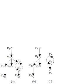
Figure 3: (a): ${\cal G}_{c}$ of a switched system with $N=2$ and $n=7$. No multiple edges exist in ${\cal G}_{c}$. (b) and (c): a generalized stem and a generalized bud that span ${\cal G}_{c}$.

Example 3

Consider a switched system with $N=2$ and $n=10$. The colored union graph ${\cal G}_{c}$ is given in Fig. 4(a), where there is no multiple edge (thus the subsystem digraphs ${\cal G}_{1}$ and ${\cal G}_{2}$ can be uniquely extracted from it). Let $(A_{1},B_{1})$ and $(A_{2},B_{2})$ be respectively the system matrices corresponding to ${\cal G}_{1}$ (solid edges) and ${\cal G}_{2}$ (dotted edges). It can be verified that ${\rm grank}[A_{1},A_{2},B_{1},B_{2}]=9$, implying that this system is not structurally controllable via Theorem 2. Furthermore, Fig. 4(b) shows that vertices $\{v_{1},...,v_{6},v_{9},v_{10}\}$ can be covered by a generalized cactus configuration. It follows from Corollary 1 that ${\rm grank}{\cal R}\geq 8$. A lower bound of ${\rm grank}{\cal R}\geq 6$ can also be obtained from Fig. 4(c), which shows that ${\cal G}_{c}$ contains a conventional cactus configuration covering $\{v_{1},...,v_{5},v_{9}\}$. A further inspection on the MDG $\hat{\cal G}_{\bar{l}}$ yields that any $\hat{V}_{U}-\hat{V}_{X0}$ linking in $\hat{\cal G}_{\bar{l}}$ for any $\bar{l}\geq 2$ has a size at most $8$. Combining it with the lower bound from Fig. 4(b), we obtain ${\rm grank}{\cal R}=8$.

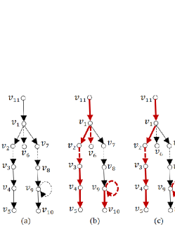
Figure 4: (a): ${\cal G}_{c}$ (no multiple edges) of a switched system with $N=2$ and $n=10$. (b): a generalized cactus configuration in ${\cal G}_{c}$ (depicted in bold red lines). (c): a conventional cactus configuration in ${\cal G}_{c}$ (bold red lines).

Example 3 shows that the lower bound for ${\rm grank}{\cal R}$ provided by Corollary 1 can be tighter than the one provided by the conventional cactus configuration covering. In addition, the upper bound provided by Proposition 1 can be tighter than the one provided by ${\rm grank}[A_{1},...,A_{N},B_{1},...,B_{N}]$. Motivated by this, we conjecture that the maximum size of state vertices that can be covered by a generalized cactus configuration in ${\cal G}_{c}$ and the maximum size of a $\hat{V}_{U}-\hat{V}_{X0}$ linking in $\hat{\cal G}_{\bar{l}}$ ($\bar{l}\geq n$) always coincide. If this conjecture is true, then Corollary 1 can determine the exact generic dimension of controllable subspaces of switched systems. Notice that when ${\rm grank}{\cal R}=n$, or when $N=1$ (i.e., for LTI systems), this conjecture is true [23, 21].

IV Extension to discrete-time systems

We extend the previous results to reversible switched discrete-time systems. This leads to not only simplified necessary and sufficient conditions for the structural controllability, but also the determination of the generic dimension of controllable subspaces.

Consider a switched discrete-time system governed by

$$x(k+1)=A_{\sigma(k)}x(k)+B_{\sigma(k)}u(k),$$ (7)

where $\sigma:\{0,1,...\}\to\{1,2...,N\}$ is the switching path, $x(k)\in{\mathbb{R}}^{n}$, $u(k)\in{\mathbb{R}}^{m_{\sigma(k)}}$. Like the continuous-time case, $(A_{i},B_{i})$ is called the subsystem of (7), $i=1,...,N$. In a switching path $\sigma$, $\sigma(k)=i$ implies that subsystem $(A_{i},B_{i})$ is chosen as the system realization.

Definition 9

[6] System (7) is said to be controllable, if for any $x\in{\mathbb{R}}^{n}$, there exists a finite $M$, a switching path $\sigma(k):\{0,...,M-1\}\to\{1,...,N\}$, and input $u(k)\in{\mathbb{R}}^{m_{\sigma(k)}}$ for $k=0,...,M-1$, such that $x(0)=x$ and $x(M)=0$.

Like [8, 24], we assume that system (7) is reversible, i.e., $A_{i}$ is non-singular for $i=1,...,N$. According to [25], it is possible to represent any causal discrete-time system (input-output) through a reversible state variable representation. Moreover, sampled data systems are naturally reversible. Therefore, reversible system representation is very general and applicable to a wide range of systems. On the other hand, as shown in [6, Theo 1, 2], criteria for controllability of non-reversible systems require checking an infinite number of switching paths. While for the class of reversible systems, its controllability can be characterized as follows.

Lemma 4

For a reversible system (7), it is controllable if and only if the following controllability matrix ${\cal R}$ has full row rank:

$${\cal R}=\left[A_{i_{n}}^{j_{n}}A_{i_{n-1}}^{j_{n-1}}\cdots A_{i_{1}}^{j_{1}}B_{i_{1}}|_{i_{1},...,i_{n}=1,...,N}^{j_{n},...,j_{1}=0,...,n-1}\right].$$

Moreover, the dimension of the controllable subspaces is ${\rm rank}{\cal R}$.

Structural controllability of the discrete-time system (7) is defined in the same way as it is for the continuous-time system (1). Observe that the controllability matrix in Lemma 4 is of the same form as that in Lemma 1. This means the methods and results in the previous section can be directly applied to reversible switched discrete-time systems. However, by leveraging the reversible structure, some deeper insights can be obtained. In what follows, all graph-theoretic notions and notations are the same as in the continuous-time case.

Theorem 3

The generic dimension of controllable subspaces of the reversible system (7) equals the number of input-reachable state vertices in ${\cal G}_{c}$.

Proof:

Let $X_{\rm re}\subseteq X$ be the input-reachable state vertex set in ${\cal G}_{c}$. By the construction of $W_{\bar{l}}$ ($\bar{l}\geq n$), any linking from $\hat{V}_{U}$ to $\hat{V}_{X0}$ has a size upper bounded by $|X_{\rm re}|$. From Proposition 1, ${\rm grank}{\cal R}$ is no more than the maximum size of a $\hat{V}_{U}-\hat{V}_{X0}$ linking in $\hat{\cal G}_{\bar{l}}$, thus upper bounded by $|X_{\rm re}|$.

Since system (7) is reversible, ${\rm grank}A_{i}=n$ for $i=1,...,N$. It follows that there are $n$ S-disjoint edges consisting of only edges from $E_{XX}$ in ${\cal G}_{c}$. From the proof ‘(a)$\Rightarrow$(b)’ of Theorem 2, ${\cal G}_{c}$ contains a collection of vertex-disjoint cycles covering $X$. Notice that all vertices of a cycle are either input-reachable simultaneously, or not input-reachable simultaneously. Therefore, $X_{\rm re}$ can be covered by a collection of input-reachable vertex-disjoint cycles (generalized buds). It follows from Corollary 1 that ${\rm grank}W_{\bar{l}}\geq|X_{\rm re}|$, i.e., ${\rm grank}{\cal R}\geq|X_{\rm re}|$. Taking both bounds together, we obtain ${\rm grank}{\cal R}=|X_{\rm re}|$. ∎

Corollary 2

The reversible system (7) is structurally controllable, if and only if each $x\in X$ is input-reachable in ${\cal G}_{c}$.

Proof:

Immediate from Theorem 3. ∎

V Conclusions

In this paper, we have investigated the structural controllability of switched continuous time systems and reversible switched discrete time systems. By introducing new graph-theoretic concepts such as multi-layer dynamic graphs, generalized stems, buds, cactus, and cactus walking, we provide a novel generalized cactus configuration based criterion for structural controllability, which extends Lin’s graph-theoretic condition to switched systems for the first time. This not only fixes a gap in the existing literature regarding the proof of a pivotal criterion for structural controllability, but also yields a lower bound for the generic dimension of controllable subspaces (which is conjectured to be exact). Additionally, we present extensions to reversible switched discrete-time systems, leading to the determination of the generic dimension of controllable subspaces. Our future work will consist of proving or disproving the conjecture made in this paper and finding a computationally efficient way to compute the maximum size of state vertices that can be covered by generalized cactus configurations.

References

- [1] D. Liberzon, A. S. Morse, Basic problems in stability and design of switched systems, IEEE Control Systems Magazine 19 (5) (1999) 59–70.
- [2] K. S. Narendra, J. Balakrishnan, Adaptive control using multiple models, IEEE Transactions on Automatic Control 42 (2) (1997) 171–187.
- [3] L. T. Conner Jr, D. P. Stanford, The structure of the controllable set for multimodal systems, Linear Algebra and its Applications 95 (1987) 171–180.
- [4] Z. Sun, S. S. Ge, T. H. Lee, Controllability and reachability criteria for switched linear systems, Automatica 48 (5) (2002) 775–786.
- [5] Z. Sun, S. S. Ge, Analysis and synthesis of switched linear control systems, Automatica 41 (2) (2005) 181–195.
- [6] S. S. Ge, Z. Sun, T. H. Lee, Reachability and controllability of switched linear discrete-time systems, IEEE Transactions on Automatic Control 46 (9) (2001) 1437–1441.
- [7] G. Xie, L. Wang, Controllability and stabilizability of switched linear-systems, Systems & Control Letters 48 (2) (2003) 135–155.
- [8] Z. Ji, H. Lin, T. H. Lee, A new perspective on criteria and algorithms for reachability of discrete-time switched linear systems, Automatica 45 (6) (2009) 1584–1587.
- [9] D. P. Stanford, L. T. Conner, Jr, Controllability and stabilizability in multi-pair systems, SIAM Journal on Control and Optimization 18 (5) (1980) 488–497.
- [10] Y. Y. Liu, J. J. Slotine, A. L. Barabasi, Controllability of complex networks, Nature 48 (7346) (2011) 167–173.
- [11] X. Liu, H. Lin, B. M. Chen, Structural controllability of switched linear systems, Automatica 49 (12) (2013) 3531–3537.
- [12] C. T. Lin, Structural controllability, IEEE Transactions on Automatic Control 19 (3) (1974) 201–208.
- [13] J. M. Dion, C. Commault, J. Van DerWoude, Generic properties and control of linear structured systems: a survey, Automatica 39 (2003) 1125–1144.
- [14] G. Ramos, A. P. Aguiar, S. D. Pequito, An overview of structural systems theory, Automatica 140 (2022) 110229.
- [15] S. Pequito, G. J. Pappas, Structural minimum controllability problem for switched linear continuous-time systems, Automatica 78 (2017) 216–222.
- [16] Y. Zhang, Y. Xia, S. Liu, Z. Su, On polynomially solvable constrained input selections for fixed and switched linear structured systems, Automatica, in press, 2023.
- [17] S. S. Mousavi, M. Haeri, M. Mesbahi, Strong structural controllability of networks under time-invariant and time-varying topological perturbations, IEEE Transactions on Automatic Control 66 (3) (2020) 1375–1382.
- [18] M. Pósfai, P. Hövel, Structural controllability of temporal networks, New Journal of Physics 16 (12) (2014) 123055.
- [19] Y. Zhang, Y. Xia, L. Wang, On the reachability and controllability of temporal continuous-time linear networks: A generic analysis, arXiv preprint arXiv:2302.11881,2023.
- [20] C. T. Lin, Structural controllability, IEEE Transactions on Automatic Control 48 (3) (1974) 201–208.
- [21] S. Poljak, On the generic dimension of controllable subspaces, IEEE Transactions on Automatic Control 35 (3) (1990) 367–369.
- [22] K. Murota, S. Poljak, Note on a graph-theoretic criterion for structural output controllability, IEEE Transactions on Automatic Control 35 (8) (1990) 939–942.
- [23] S. Hosoe, Determination of generic dimensions of controllable subspaces and its application, IEEE Transactions on Automatic Control 25 (6) (1980) 1192–1196.
- [24] Y. Zhu, Z. Sun, Stabilizing design for discrete-time reversible switched linear control systems: A deadbeat control approach, Automatica 129 (2021) 109617.
- [25] M. Fliess, Reversible linear and nonlinear discrete-time dynamics, IEEE Transactions on Automatic Control 37 (1992) 1144–1153.