Lagrangian descriptors and their applications to deterministic chaos

Abstract.

We present our recent contributions to the theory of Lagrangian descriptors for discriminating ordered and deterministic chaotic trajectories. The class of Lagrangian Descriptors we are dealing with is based on the Euclidean length of the orbit over a finite time window. The framework is free of tangent vector dynamics and is valid for both discrete and continuous dynamical systems. We review its last advancements and touch on how it illuminated recently Dvorak’s quantities based on maximal extent of trajectories’ observables, as traditionally computed in planetary dynamics.

1. Introduction

This present short presentation aims at summarising our recent contributions to the theory of Lagrangian Descriptors (LDs) for deterministic chaos detection. It is predominantly based on Daquin et al., (2022) and Daquin and Charalambous, (2023) to which we refer for a comprehensive literature review. LDs are scalar quantities rooted in fluid mixing and coined as such by Mendoza and Mancho, (2010). There were initially introduced by Madrid and Mancho, (2009) for vector fields. Consider the autonomous regular vector field

(1) $$\dot{x}=v(x),\,x\in\mathbb{R}^{n},$$

and the orbit associated to Eq. (1) starting at $x_{0}\in\mathbb{R}^{n}$ at $t=0$. Its LD at time $T>0$ is defined as

(2) $$\textrm{LD}(x_{0};T)=\int_{0}^{T}\left\lVert v\big{(}x(s)\big{)}\right\rVert_{2}\,\textrm{d}s,$$

and corresponds to the Euclidean arc-length of the trajectory over the time-window $[0,T]$. LDs have been generalised by considering the integration of others bounded and intrinsic observable associated to an orbit (Mancho et al.,, 2013). We stick here to the LD based on the arc-length method. Extending LDs to discrete systems is straightforward. Let us denote by $\{z_{0},z_{1},\dots,z_{N}\}$, $z_{j}\in\mathbb{R}^{m}\,j=0,\cdots,N$, a finite orbit associated to a discrete mapping $f$, $z_{j}=f^{j}(z_{0}),j=1,\cdots,N$. The LD associated to such orbit is given by

(3) $$\textrm{LD}(z_{0};N)=\sum_{j=0}^{N-1}\sqrt{\sum_{l=1}^{m}(z_{j+1}^{(l)}-z_{j}^{(l)})^{2}},$$

where $z_{j}^{(l)}$ denotes the $l$-th component of the state $z$ at time $j$.

The rest of this contribution is organised as follows. In Sect. 2, we highlight the phenomenology of the LDs for chaos detection by presenting new applications to the paradigmatic one-dimensional logistic map. Sect. 3 presents the finite-time chaos indicator we have derived from LDs computations and discuss the models on which it has been successfully employed so far. Sect. 4 connects the LD framework with maximal excursions traditionally computed in celestial mechanics in the context of stability maps. Sect. 5 closes the paper with conclusive remarks.

2. Lagrangian Descriptors applied to the logistic model

We consider the one-dimensional quadratic logistic map (see e.g., May, (1976)) as a testing ground to illustrate the LDs concepts. The mapping is defined by

(4) $$x_{n+1}=\mathcal{L}_{\mu}(x_{n})=\mu x_{n}(1-x_{n}).$$

The state space of the dynamics is $M=[0,1]$ for $0<\mu\leq 4$ and $n\in\mathbb{N}$. Dealing with the orbit $\{x_{0},x_{1},\dots,x_{N}\}$, Eq. (5) becomes

(5) $$\textrm{LD}(x_{0};N)=\sum_{i=0}^{N-1}|x_{i+1}-x_{i}|.$$

The top panel of Fig. 1 shows the bifurcation diagram of the logisitc map for $2.9\leq\mu\leq 4$ with fixed $x_{0}=0.15$. It highlights the presence of periodic orbits, the chain of bifurcation occurring in the dynamics as $\mu$ is varied, periodic windows immersed within aperiodic range of motions. Such a window is exemplified around $\mu=3.63$ and will be further discussed. The middle panel of Fig. 1 shows the value of the finite time Lyapunov exponent (FTLE) computed at time $N=10^{6}$ as a function of $\mu$. The FTLE is defined as

(6) $$\lambda(x_{0};N)=\frac{1}{N}\log_{10}\big{(}\prod_{i=0}^{N}|D\mathcal{L}_{\mu}(x_{i})|\big{)}=\frac{1}{N}\sum_{i=0}^{N}\log_{10}(|\mu(1-2x_{i})|).$$

We have colored the final value of $\lambda$ according to its sign. Negative FTLEs appear in blue and correspond to regular motions. The values $\lambda=0$ indicate bifurcations. The positive FTLEs appear in red and correspond to orbits with sensitive dependence upon the initial conditions, i.e., chaotic motions. Interestingly enough, there is a sharp link between the values of the FTLEs and properties of the LD map. In fact, the bottom panel of Fig. 1 shows the LD landscape (computed also at the final time $N=10^{6}$), colored according to the final value of $\lambda$. We observe that negative $\lambda$’s correspond to smooth parts of the LD curve, whilst positive $\lambda$’s correspond to domains where the LD metric is irregular. Fig. 2 repeats the computations of FTLEs and LDs at a much thinner scale of the control parameter $\mu$ (the shaded area around $\mu=3.63$ highlighted in Fig. 1) and further confirm our former observations. This demonstrates the sensitivity and robustness of the regularity of the LD metric as diagnostic for chaos detection. For $\mu=4$, $\mathcal{L}_{4}$ is chaotic for every $x_{0}$ (May,, 1976; Banks et al.,, 2003). Fig. 3 shows the LD landscape for varying $x_{0}$ in $(0,1)$ with fixed $\mu=4$ at $N=10^{4}$. The obtained landscape is nowhere smooth, in accordance with the former numerical results.

Figure 1. Bifurcation diagram (top panel), Lyapunov exponents (middle panel) and LD lengths (bottom panel) of the logistic equation when $\mu$ is varied. There is a strong connection between the regularity of the orbits (sign of Lyapunov exponent) and the regularity of the LD map. See text for further details.

Figure 2. Computation of Lyapunov exponents $\lambda$ and LD lengths on a small range of the control parameter $\mu$. The regularity of the length application provides a very sensitive and reliable indicator of the ordered and chaotic nature of the motion.

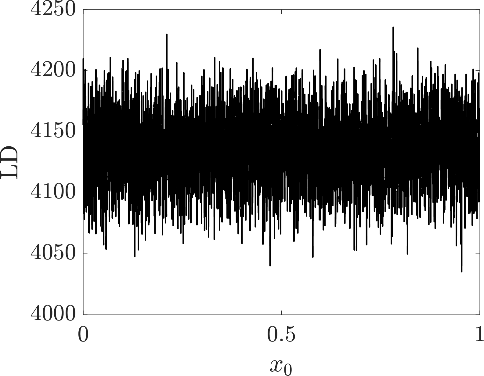
Figure 3. Landscape of LDs as a function of $x_{0}$ for the logistic map with $\mu=4$. For this parameter, the map is known to be chaotic. This is reflected in the absence of regularity of the LD metric.

3. The new non-variational geometrical chaos indicators

As just illustrated on the logistic model, the regularity of the LD metric keeps trace of the possible chaotic nature of the orbit. This property has also been observed on a series of integrable and non-integrable mechanical models supporting interacting resonances (Daquin et al.,, 2022). For integrable 1-degree-of-freedom (DoF) systems, Pédenon-Orlanducci et al., (2022) showed that the rate of divergence of the derivative of the length metric (using a time-free parametrisation of LDs) scales as a power law when crossing transversally separatrices. The scaling obeys $\mathcal{O}(1/\sqrt{E})$, where $E$ is the energy labelling the level curve. Those observations led us to assume that the LD map is $\mathcal{C}^{\infty}$ on the set $\mathcal{R}$ of regular motions. Leveraging on this, Daquin et al., (2022) introduced the $\left\lVert\Delta\textrm{LD}\right\rVert$ index measuring the regularity of the LD metric through second-derivatives estimates, similarly to the frequency analysis method (Laskar,, 1993). For the dimension $n=1$ and a point $y\in\mathcal{R}$, $\left\lVert\Delta\textrm{LD}\right\rVert$ is defined as

(7) $$\left\lVert\Delta\textrm{LD}\right\rVert(y;T)=|\textrm{LD}^{{}^{\prime\prime}}(y;T)|.$$

Numerically, the second derivative in Eq. (7) is estimated by finite differences of the type

(8) $$|\textrm{LD}^{{}^{\prime\prime}}(y;T)|\simeq\frac{|\textrm{LD}(y+h;T)+\textrm{LD}(y-h;T)-2\textrm{LD}(y;T)|}{h^{2}},$$

for a small enough discretisation step $h$. The $\left\lVert\Delta\textrm{LD}\right\rVert$ index is proposed as new chaos indicator and undergoes sharp increases on the complement set $\mathcal{R}^{C}$ of $\mathcal{R}$ when crossing transversally separatrices of integrable model or hyperbolic domains of non-integrable models (Daquin et al.,, 2022). In the more general case ($n>1$), $\left\lVert\Delta\textrm{LD}\right\rVert$ reads as

(9) $$\left\lVert\Delta\textrm{LD}\right\rVert(y;T)=\sum_{i=1}^{n}|\partial_{y^{(i)}y^{(i)}}^{2}\textrm{LD}(y;T)|.$$

The $\left\lVert\Delta\textrm{LD}\right\rVert$ index has been applied and benchmarked on several low-dimensional models to derive stability maps computed on fine domains of initial conditions or parameter space, including: the $2$ dimensional standard map and higher $4$ dimensional coupled standard maps, non-autonomous pendulum-like models having resonant junctions and interactions supporting resonant webs, as ubiquitous in celestial mechanics. The $\left\lVert\Delta\textrm{LD}\right\rVert$ keeps trace of manifolds’ oscillations when computed on a short timescale, as observed on the $2$-DoF Hénon-Heiles model (Daquin et al.,, 2022). Qualitative comparison with established variational methods (e.g., the FLI, MEGNO, SALI) have shown excellent agreements in disentangling ordered and chaotic orbits. Recently, quantitative oriented analysis of the performance of LD like diagnostics have been investigated (Hillebrand et al.,, 2022; Zimper et al.,, 2023). On $4D$ coupled standard maps in a mixed phase space regime, it has been shown that the probability of agreement $P_{A}$ in the discrimination of the orbit against the SALI index is on the order of $90\%$. Thus, the $\left\lVert\Delta\textrm{LD}\right\rVert$ index is a cheap, easily implementable and reliable tool for detecting separatrices and chaotic motions.

4. Diameters and Dvorak’s amplitudes

The LDs just presented are based on the length of the orbit, see Eq. (3) and (5). For bounded orbits, the amplitude (or diameter) is another geometrical quantity that might be considered. Consider Eq. (1), a trajectory $x(t;x_{0})$ with initial condition $x_{0}$ and an observable $\phi$. The diameter on the finite time segment $[0,T]$ along the observable $\phi$ is defined as

(10) $$D(x_{0};T)=\max_{0\leq\tau\leq T}\phi\big{(}x(\tau;x_{0})\big{)}-\min_{0\leq\tau\leq T}\phi\big{(}x(\tau;x_{0})\big{)},$$

with similar definitions for the discrete case. The diameter $D$ is called maximal shift in Mundel et al., (2014). The study of its cumulative distribution function demonstrated relevance to characterise fluid mixing properties, and is certainly an interesting direction of future research. Daquin and Charalambous, (2023) considered diameters of $n$-DoF Hamiltonian systems by looking more specifically at the diameter of the actions. It turns out that LD and D maps share analogies, and of practical interest is the loss of regularity when crossing separatrices or chaotic layers transversally. This led to introduce the analogue of Eq.(9) for the diameter of Eq. (10), denoted $\left\lVert\Delta D\right\rVert$. Diameters like quantities have been computed for a while in planetary dynamics in the context of stability maps, by focusing on stretches of some keplerian elements $a$, $e$ or $i$ (respectively semi-major axis, eccentricity and inclination), usually denoted by $\delta a$, $\delta e$ or $\delta i$, see e.g., Dvorak et al., (2004); Sándor et al., (2007). In the context of $2$ and $3$-body co-planar simulations triggered towards mean-motion resonances, Daquin and Charalambous, (2023) shown in particular how the $\left\lVert\Delta D\right\rVert$ maps supplements the traditional diameter analysis, allowing to reinflate and recover sharply separatrices, detect thin chaotic lines and the web of resonances, otherwise undetected with the classical diameter metric. As for $\left\lVert\Delta\textrm{LD}\right\rVert$, $\left\lVert\Delta D\right\rVert$ is a cheap non-variational geometrical index allowing sensitive chaos detection.

5. Conclusive remarks

This short manuscript has presented and summarised our latest contributions to the theory of Lagrangian Descriptors for chaos detection. A finite-time non-variational chaos indicator can be easily derived from the the study of the regularity of length map. For this, we suggested a second-derivatives based index. We have discussed connection of Lagrangian diagnostics with quantities employed to characterise fluid flow mixing and diameter quantities encountered in celestial mechanics. The Lagrangian framework offers a convenient mold for detecting chaos without the need of deriving the variational equations, possibly leading to substantial implementation reduction. Our current efforts focus on the quantitative assessments of their performances.

References

- Banks et al., (2003) Banks, J., Dragan, V., and Jones, A. (2003). Chaos: a mathematical introduction, volume 18. Cambridge University Press.
- Daquin and Charalambous, (2023) Daquin, J. and Charalambous, C. (2023). Detection of separatrices and chaotic seas based on orbit amplitudes. Celestial Mechanics and Dynamical Astronomy, 135(3):1–18.
- Daquin et al., (2022) Daquin, J., Pedenon-Orlanducci, M., Agaoglou, M., Garcia-Sanchez, G., and Mancho, A. M. (2022). Global dynamics visualisation from Lagrangian Descriptors. Applications to discrete and continuous systems. Physica D: Nonlinear Phenomena, 442:133520.
- Dvorak et al., (2004) Dvorak, R., Pilat-Lohinger, E., Schwarz, R., and Freistetter, F. (2004). Extrasolar Trojan planets close to habitable zones. Astronomy & Astrophysics, 426(2):L37–L40.
- Hillebrand et al., (2022) Hillebrand, M., Zimper, S., Ngapasare, A., Katsanikas, M., Wiggins, S. R., and Skokos, C. (2022). Quantifying chaos using Lagrangian descriptors.
- Laskar, (1993) Laskar, J. (1993). Frequency analysis for multi-dimensional systems. Global dynamics and diffusion. Physica D: Nonlinear Phenomena, 67(1-3):257–281.
- Madrid and Mancho, (2009) Madrid, J. J. and Mancho, A. M. (2009). Distinguished trajectories in time dependent vector fields. Chaos: An Interdisciplinary Journal of Nonlinear Science, 19(1):013111.
- Mancho et al., (2013) Mancho, A., Wiggins, S., Curbelo, J., and Mendoza, C. (2013). Lagrangian descriptors: A method for revealing phase space structures of general time dependent dynamical systems. Commun Nonlinear Sci Numer Simulat, 18:3530–3557.
- May, (1976) May, R. M. (1976). Simple mathematical models with very complicated dynamics. Nature, 261(5560):459–467.
- Mendoza and Mancho, (2010) Mendoza, C. and Mancho, A. (2010). Hidden geometry of ocean flows. Physical review letters, 105(3):038501.
- Mundel et al., (2014) Mundel, R., Fredj, E., Gildor, H., and Rom-Kedar, V. (2014). New Lagrangian diagnostics for characterizing fluid flow mixing. Physics of Fluids, 26(12):126602.
- Pédenon-Orlanducci et al., (2022) Pédenon-Orlanducci, R., Carletti, T., Lemaitre, A., and Daquin, J. (2022). Geometric parametrisation of Lagrangian Descriptors for 1 degree-of-freedom systems. In Pinto, C. M., editor, Nonlinear Dynamics and Complexity: Mathematical Modelling of Real-World Problems, pages 221–238. Springer International Publishing.
- Sándor et al., (2007) Sándor, Z., Süli, Á., Érdi, B., Pilat-Lohinger, E., and Dvorak, R. (2007). A stability catalogue of the habitable zones in extrasolar planetary systems. Monthly Notices of the Royal Astronomical Society, 375(4):1495–1502.
- Zimper et al., (2023) Zimper, S., Ngapasare, A., Hillebrand, M., Katsanikas, M., Wiggins, S. R., and Skokos, C. (2023). Performance of chaos diagnostics based on Lagrangian descriptors. Application to the 4D standard map. Physica D: Nonlinear Phenomena, 453:133833.