Symmetric conformity functions make decision-making processes independent of the distribution of learning strategies

Abstract

Two main procedures characterize the way in which social actors evaluate the qualities of the options in decision-making processes: they either seek to evaluate their intrinsic qualities (individual learners) or they rely on the opinion of the others (social learners). For the latter, social experiments have suggested that the mathematical form of the probability of adopting an option, called the conformity function, is symmetric in the adoption rate. However, the literature on decision making includes models where social learners employ either symmetric and non-symmetric conformity functions. Here, we generalize previous models and show analytically that when symmetric conformity functions are considered, the form of the probability distribution of the individual strategies (behaving as a social or an individual learner) does not matter: only the expected value of this distribution influences the determination of the steady state. Moreover, we show that a dynamics that considers strategies as idiosyncratic properties of the agents and another that allows them to change in time lead to the same result in the case of symmetric conformity functions, while the results differ in the case of non-symmetric ones. This fact can inspire experiments that could shed light on the debate about this point.

I Introduction

Decision making is an individual task that benefits from a detailed knowledge about the possible options. The vast literature addressing the way in which different species of animals, and in particular humans, acquire this knowledge is pluri-disciplinary and targets different aspects of the problem [1, 2, 3]. Social actors are usually classified according to their learning strategies as individual learners, those who search to identify the intrinsic merits of the options without suffering any peer pressure, or social learners, those who simply follow their peers’ choice. However, this is a rough classification as each class entails a variety of cognitive processes that are very difficult to disentangle experimentally. Early studies on decision making were challenged by new experimental techniques [4, 5]. A question that raised strong debates concerns the transmission of learning abilities, in the light of natural selection. As social learning (in any of its forms) is considered less costly than individual learning, it is supposed to enhance individual fitness and then prevail [6]. However, A. Rogers showed that this may not be the case if the environment is subject to changes. In this case, if social learners are selected, their proportion in society increases, and the probability that they obtain a wrong information about the environment by copying other social learners with “old” information increases, and therefore, their fitness diminishes. This is known as the Rogers’ paradox [7]. Rogers’ paradox does not mean that social learning—thus culture—prevents social agents from adapting to the environment, it just points out that a model that only evaluates the cost-benefit of the chosen strategies is not enough to account for the observations. Rogers himself had suggested to introduce some biases in the social learning like to copy preferentially high fitness individuals, or as proposed by Boyd and Richerson, just copy individual learners. Neither of the two lifted the paradox, and the fitness of the group decreases with generations because the strategy of social learners is frequency dependent while that of individual learners is not [8]. Other modifications introduce the possibility for the strategies of an individual to evolve according to different situations (cost of individual learning, changing environment, fitness of the neighbours, etc.). These modifications may lift Rogers’ paradox or not depending on details of the parameters [9, 10]. All this shows that the problem of how learning strategies are transmitted goes beyond a cost-benefit problem and that flexibility in the learning strategies is essential in order to maintain a high fitness of the population.

Another aspect of the problem would be to ask how a given generation composed of individual and social learners reaches a collective decision. In this case, the particular ways in which both social and individual learners acquire new knowledge are studied. For example, one can consider that social learners conform to an option because of peer pressure. Individual learners, who seek information on their own about the options, may also take advantage of the knowledge about the choices of others but in a different way, as the merit of an option may in some cases, be correlated to the number of individuals that have already chosen it, either positively or negatively [11]. Let us consider for example the usage of electric cars. Individual learners may consider that part of the merit of this option resides in that it limits the $CO_{2}$ emissions, but they may also be interested in learning that a large fraction of the population has already adopted it because this will enhance the development of recharging stations, increasing the merit of this option further. On the contrary, if they were to decide about choosing public transportation, which also reduces $CO_{2}$ emission, they may also evaluate the fact that if a large fraction of others already chose this option, its merit diminishes because of the discomfort of crowded transportation. In this sense, the merit of the options is not a constant but may be dependent on the frequency. It is interesting to notice here that this point also addresses the main ingredient of Rogers’ paradox [8].

Recently, a dynamical system model has showed that social learners may, when numerous, impair collective performance [12]. This model considers the proportion of social and individual learners as well as the value of the merit as a fixed parameter of the model and chooses a symmetric conformity function to describe social learning. However, the specific form of social learning function is still a subject of study. McElreath et al. have detailed different heuristics for social learning which lead to either symmetric or non-symmetric functional forms [13]. Experiments, both in laboratory and in real settings, show different ways in which individuals learn from peers [14] and whether there is a general mathematical form representing a general social learning function is far from being clear [15, 16]. These experiments also observed the situation where subjects change their strategies during the experiment [16] alternating the ways in which they gather information (either by learning individually or by getting information from their peers).

In this work, we present a general theoretical model that allows us to explore analytically the possible outcomes of dynamics based either on fixed (quenched dynamics) or alternating learning strategies (annealed dynamics), and where the social learning function may be symmetric, as the one considered in Ref. [12], or non-symmetric, as in the well-known $q$-voter model [17]. The model also allows for a general distribution of such strategies, $f_{p}(p_{i})$, where $p_{i}$ is the probability that a given agent acts as an individual learner. We show analytically that a symmetric learning function has important consequences in the phase diagram of the system, which does not depend on the distribution $f_{p}(p_{i})$, but only on its first moment, $\bar{p}$. Moreover, in this situation, the phase diagrams of the quenched and annealed dynamics are identical. On the contrary, for the non-symmetric learning function the resulting phase diagrams for the quenched and annealed dynamics are different, even with variations in the presence of discontinuous or continuous transitions depending on the parameters.

Our results confirm and extend those presented in Ref. [12] which is a particular case of our model for a given set of parameters.

II model and methods

We study the situation where individuals (agents) of the society have to make a binary decision—choosing a product, adopting a given behaviour, or a social norm—where the options are called $A$ and $B$. Those who behave as individual learners evaluate the options’ properties by themselves, while social learners rely on what has been chosen by others. Each agent $i$ chooses to behave as an individual learner with probability $p_{i}$ and the distribution of such probabilities over the population may follow a general distribution $f_{p}(p_{i})$, as illustrated in the left part of Fig. 1. There are two possible dynamics: either the agents choose their $p_{i}$ from the start and stay with them throughout the entire dynamical learning process (quenched dynamics), or the agents choose their $p_{i}$ at each step of the dynamics (annealed dynamics).

An agent that follows the individual learner dynamics will evaluate the probability of choosing one of the options, let’s say $A$, using the function $f_{I}(a)$, where $a$ represents the fraction of the population that has chosen that option. Therefore, the probability of selecting option $B$ through the same process is given by the complementary probability $1-f_{I}(a)$. At a difference with previous works, we use an individual learning function, instead of a constant parameter, to account for the situation where the merit of the option may increase or decrease according to the fraction of the population that has already adopted it [11]. Following the Rasch model [18], we use the logit function to define $f_{I}(a)$. Thus, the natural logarithm of the odds of choosing $A$ is proportional to the fraction of individuals favoring this option over the fraction $a_{m}$, which gives the equal probability to both options:

$$\ln\left[\frac{f_{I}(a)}{1-f_{I}(a)}\right]=k(a-a_{m}).$$ (1)

The parameter $k$ accounts for the tendency and the strength of the likelihood of choosing option $A$, whereas $a_{m}$ is the midpoint of $f_{I}(a)$, i.e., $f_{I}(a_{m})=1/2$, which we set here as $a_{m}=1/2$.

The left hand side of Eq. (1) can be interpreted as a trade-off between an individual’s attitudes towards option $A$ and its adoption difficulties [19, 20]. In our model, this trade-off depends explicitly on the number of adopters. From Eq. (1), we get the following form of the individual leaning probability:

$$f_{I}(a)=\frac{1}{1+e^{-k(a-a_{m})}}.$$ (2)

The right panel of Fig. 1 illustrates the shape of $f_{I}(a)$ for different values of $k$. Notice that the model studied in Ref. [12] is a particular case of this one for $k=0$ and quenched dynamics.

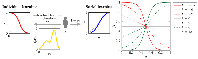
Figure 1: Main elements of the model. (left panel) Model’s diagram: agent $i$ has a personal inclination towards individual learning, represented by the probability $p_{i}$ of choosing this strategy. Its value is drawn from distribution $f_{p}(p_{i})$. In the quenched dynamics a $p_{i}$ value is asigned to agent $i$ at the beginning of the process; alternatively in the annealed dynamics, the tendency to individual learning may change at each time step. Both learning strategies depend on the fraction of opinion $A$ followers, $a$. (right panel) Individual learning as a function of the fraction of option $A$ followers for a few values of $k$.

On the other hand, social learners will be directly influenced by the choice of their peers. The form of this influence is given by a conformity function $f_{S}(x)$ that returns the probability of changing to the option favored by a fraction $x$ of individuals. This function accounts for the average social influence felt by the agent, which is growing with the fraction of adopters of the option. Table 1 summarises the way individual and social learning functions are used to update the agents’ options.

Table 1: Probabilities that an agent with a given option remains it or changes it to the alternative one using a corresponding learning strategy.

Option before learning	Option after
	Individual learning		Social learning
	$A$	$B$	$A$	$B$
$A$	$f_{I}(a)$	$1-f_{I}(a)$	$1-f_{S}(1-a)$	$f_{S}(1-a)$
$B$	$f_{I}(a)$	$1-f_{I}(a)$	$f_{S}(a)$	$1-f_{S}(a)$

The mathematical properties of the conformity function are still a subject of debate. In simple models of frequency-dependent bias [6], the conformity function is taken to be an increasing function, symmetric around a midpoint $f_{S}(0.5)=0.5$. Some experimental results tend to support this hypothesis [14, 13, 21]. For such a conformity function, the following dependency holds:

$$f_{S}(x)+f_{S}(1-x)=1$$ (3)

for all $x\in\left[0,1\right]$. Other works have represented social influence through non-symmetric conformity functions [22, 6, 23]. There is also experimental evidence for such a form, in particular concerning what is know as frequency-dependent direct bias in social learning [6, 16, 13]. Thus, we study both cases in this work. For the symmetric case, and for the sake of comparison, we use the same form as in Ref. [12]:

$$f_{S}(x)=\begin{cases}\frac{1}{2}(2x)^{q}&\text{if }0\leq x<0.5,\\ 1-\frac{1}{2}\left[2(1-x)\right]^{q}&\text{if }0.5\leq x\leq 1.\end{cases}$$ (4)

For the non-symmetric conformity functions, we assume a simple mathematical form inspired from the non-linear q-voter model [17, 23, 24]:

$$f_{S}(x)=x^{q}.$$ (5)

Both these functions are parameterized by $q$, which reflects their degree of non-linearity, where $q=1$ corresponds to a linear response.

III Results

We study two dynamical scenarios where $p_{i}$ is either a quenched or annealed property of agent $i$ [23, 24]. In this section, we present the general equations for these two dynamics without imposing any specific form of the learning strategy distribution, $f_{p}(p_{i})$. We also illustrate the behaviour of the system in the particular case treated in Ref. [12], where the choice between the two strategies follows a simple Bernoulli distribution. These general results along with their specification for the individual and social learning functions, given by Eq. (2), Eq. (4), and Eq. (5), are summarized below in Table 2.

III.1 General results

Let $f_{p}(x)$ be an arbitrary distribution with mean $\bar{p}=\int xf_{p}(x)dx$.

III.1.1 Annealed dynamics

At each time step, each agent is assigned a probability of being individual learner from the distribution $f_{p}(p_{i})$. It should be noticed that the probability distribution itself does not change in time.

The time evolution of the fraction of adopters of choice A, $a$, is given by:

$$\frac{da}{dt}=P_{B\rightarrow A}(1-a)-P_{A\rightarrow B}a,$$ (6)

where $P_{B\rightarrow A}$ and $P_{A\rightarrow B}$ are the transition probabilities. The transition probabilities from one option to the other are formed at each step by those agents that learnt about the options either individually or socially:

$$\begin{split}P_{B\rightarrow A}=&\int xf_{I}(a)f_{p}(x)dx+\int(1-x)f_{S}(a)f_{p}(x)dx,\\ P_{A\rightarrow B}=&\int x\left[1-f_{I}(a)\right]f_{p}(x)dx\\ &+\int(1-x)f_{S}(1-a)f_{p}(x)dx.\end{split}$$ (7)

Having integrated the above formulas, we get:

$$\begin{split}P_{B\rightarrow A}&=\bar{p}f_{I}(a)+(1-\bar{p})f_{S}(a),\\ P_{A\rightarrow B}&=\bar{p}\left[1-f_{I}(a)\right]+(1-\bar{p})f_{S}(1-a).\end{split}$$ (8)

From Eqs. (6) and (8), we get that

$$\frac{da}{dt}=\bar{p}\left[f_{I}(a)-a\right]+(1-\bar{p})\left[(1-a)f_{S}(a)-af_{S}(1-a)\right].$$ (9)

Calling $a^{*}$ the fixed points that make:

$$\left.\frac{da}{dt}\right|_{a^{*}}=0.$$ (10)

We get $a^{*}=1/2$ for any value of $\bar{p}$, and also those satisfying the following equation:

$$\bar{p}=\frac{a^{*}\left[f_{S}(a^{*})+f_{S}(1-a^{*})\right]-f_{S}(a^{*})}{a^{*}\left[f_{S}(a^{*})+f_{S}(1-a^{*})\right]-f_{S}(a^{*})+f_{I}(a^{*})-a^{*}}.$$ (11)

If the conformity function, $f_{S}(a)$, is symmetric, we can use Eq. (3) to simplify the above formula. As a result, Eq. (11) becomes:

$$\bar{p}=\frac{a^{*}-f_{S}(a^{*})}{f_{I}(a^{*})-f_{S}(a^{*})}.$$ (12)

Table 2: Summary of the results. Formulas for the fixed points with majoritarian option of the models with different dynamics and types of conformity functions.

Conformity function	Annealed dynamics	Quenched dynamics
Symmetric	Annealed and quenched dynamics lead to the same fixed points that do not depend on the full distribution of learning strategies, but only on its mean: $$\bar{p}=\frac{a^{*}-f_{S}(a^{*})}{f_{I}(a^{*})-f_{S}(a^{*})},\text{ where }\bar{p}=\int xf_{p}(x)dx.$$ (13) For a special case of symmetric conformity function given by Eq. (4), we have $$\bar{p}=\begin{dcases}\frac{2a^{*}-(2a^{*})^{q}}{2f_{I}(a^{*})-(2a^{*})^{q}}&\text{if }0\leq a^{*}<0.5,\\ \frac{2(a^{*}-1)+\left[2(1-a^{*})\right]^{q}}{2\left[f_{I}(a^{*})-1\right]+\left[2(1-a^{*})\right]^{q}}&\text{if }0.5\leq a^{*}\leq 1.\end{dcases}$$ (14)
Non-symmetric	Fixed points depend on the mean of the distribution of learning strategies: $$\bar{p}=\frac{a^{*}\left[f_{S}(a^{*})+f_{S}(1-a^{*})\right]-f_{S}(a^{*})}{a^{*}\left[f_{S}(a^{*})+f_{S}(1-a^{*})-1\right]+f_{I}(a^{*})-f_{S}(a^{*})},$$ (15) where $\displaystyle\bar{p}=\int xf_{p}(x)dx.$ For a special case of non-symmetric conformity function given by Eq. (5), we have $$\bar{p}=\frac{a^{*}(1-a^{*})^{q}-(1-a^{*})(a^{*})^{q}}{a^{*}\left[(a^{*})^{q}+(1-a^{*})^{q}-1\right]+f_{I}(a^{*})-(a^{*})^{q}}.$$ (16)	Fixed points depend on the whole shape of the distribution of learning strategies: $\begin{aligned} a^{*}&=\int a_{x}^{*}f_{p}(x)dx,\text{ where}\\ a_{x}^{*}&=\frac{xf_{I}(a^{*})+(1-x)f_{S}(a^{*})}{x+(1-x)\left[f_{S}(a^{*})+f_{S}(1-a^{*})\right]}.\end{aligned}$ For a special case of non-symmetric conformity function given by Eq. (5) and $f_{p}(x)$ given by Bernoulli distribution with mean $\bar{p}$, we have $$\bar{p}=\frac{a^{*}(1-a^{*})^{q}-(1-a^{*})(a^{*})^{q}}{f_{I}(a^{*})\left[(a^{*})^{q}+(1-a^{*})^{q}\right]-(a^{*})^{q}}.$$ (17)

III.1.2 Quenched dynamics

The probability of being an individual learner is assigned for each individual at the beginning of the dynamics, and each agent keeps the same probability value during all the evolution.

Let $a_{x}$ denote the fraction of agents that choose to act as individual learners with probability $p_{i}=x$ and who favor option $A$ and $1-a_{x}$ those who being individual learners, with the same probability, favour option $B$. For each value of the probability $x$ of being individual learner, we have the following rate equation for the adopters of $A$:

$$\frac{da_{x}}{dt}=P^{x}_{B\rightarrow A}(1-a_{x})-P^{x}_{A\rightarrow B}a_{x},$$ (18)

where $P^{x}_{B\rightarrow A}$ and $P^{x}_{A\rightarrow B}$ are the transition probabilities for the group of agents that are individual learners with probability $p_{i}=x$ (and therefore, social learners with probability $1-x$):

$$\begin{split}P^{x}_{B\rightarrow A}&=xf_{I}(a)+(1-x)f_{S}(a),\\ P^{x}_{A\rightarrow B}&=x\left[1-f_{I}(a)\right]+(1-x)f_{S}(1-a).\end{split}$$ (19)

We look for the fractions of adopters $a_{x}^{*}$ of option $A$ among agents with $p_{i}=x$ that make the evolution of all the populations stationary:

$$\left.\frac{da_{x}}{dt}\right|_{\{a_{x}^{*}\}}=0.$$ (20)

We see that $a_{x}^{*}=1/2$ is a fix point for all values of $x$, in this case, Eq. (20) is satisfied for any distribution $f_{p}(x)$. The remaining fixed points are determined by combining Eqs. (18), (19), and (20):

$$a_{x}^{*}=\frac{xf_{I}(a^{*})+(1-x)f_{S}(a^{*})}{x+(1-x)\left[f_{S}(a^{*})+f_{S}(1-a^{*})\right]},$$ (21)

where

$$a^{*}=\int a_{x}^{*}f_{p}(x)dx.$$ (22)

The fixed values of $a$ are obtained by solving Eq. (22) with the obtained formulas for $a_{x}^{*}$. If the conformity function is non-symmetric, we cannot perform further calculations without knowing the exact distribution $f_{p}(x)$. However, if the conformity function is symmetric, we can perform the integration in Eq. (22) without imposing any special form of $f_{p}(x)$ since we can use Eq. (3) to simplify Eq. (21). In such a case, we get

$$a^{*}=\bar{p}f_{\text{I}}(a^{*})+(1-\bar{p})f_{\text{S}}(a^{*}),$$ (23)

so the fixed points depend only on the mean of the distribution $\bar{p}=\int xf_{p}(x)dx$. By transforming Eq. (23), we get

$$\bar{p}=\frac{a^{*}-f_{\text{S}}(a^{*})}{f_{\text{I}}(a^{*})-f_{\text{S}}(a^{*})}.$$ (24)

Comparing Eq. (24) with Eq. (12), we get the main general result of this work: if the conformity function is symmetric, the fixed points of the quenched and the annealed dynamics are the same and only depend on the first moment of the distribution $f_{p}(p_{i})$ and not on the details of this distribution.

((a))

((b))

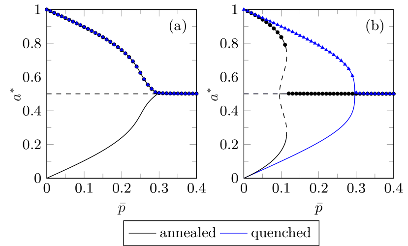
Figure 2: Stable (solid lines) and unstable (dashed lines) fixed points for the model with $q=3$ and $k=-15$ for (a) a symmetric conformity function and (b) a non-symmetric conformity function. For the symmetric conformity function, annealed and quenched approaches produce the same diagrams. Symbols represent the results from the simulations of the model with $\bullet$ annealed and $\blacktriangle$ quenched dynamics. Detailed information about the simulations can be found in the Supporting Information.

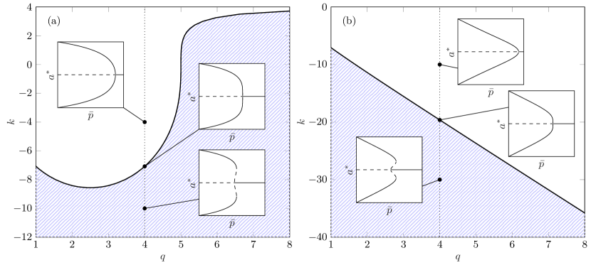
Figure 3: Phase diagrams for the model with a non-symmetric conformity function and (a) annealed (b) quenched dynamics. White and blue areas indicate regions of parameter space where only continuous and discontinuous transitions take place, respectively. Insets illustrate fixed point diagrams in given regions. More detailed versions of these figures are presented in the Supporting Information.

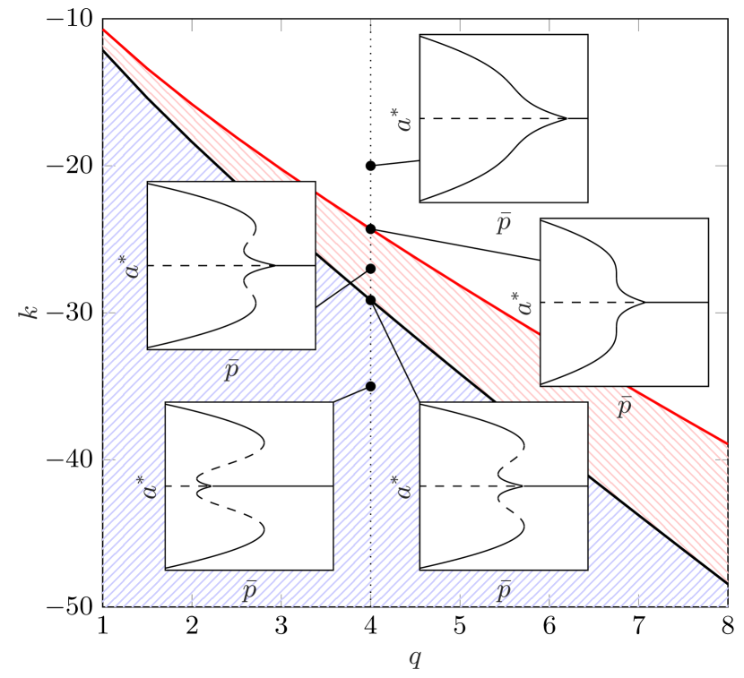
Figure 4: Phase diagram for the model with a symmetric conformity function. In this case, annealed and quenched dynamics produce the same fixed point diagrams. In white area, only continuous phase transitions take place. In red area, discontinuous phase transitions between ordered phases additionally occur. In blue area, discontinuous phase transitions between ordered and disordered phases are also possible. Insets illustrate fixed point diagrams in given regions. More detailed versions of these figures are presented in the Supporting Information.

III.2 Particular case: Bernoulli distribution of the learning strategies

Let us consider a simple case where $p_{i}$ is Bernoulli distributed, so $\forall i=1,...,N$, $f_{p}(p_{i}=1)=p$ and $f_{p}(p_{i}=0)=1-p$, and $p$ is the mean of the distribution. Note that agents with $p_{i}=1$ certainly behave as individual learners, whereas those with $p_{i}=0$ certainly behave as social learners.

III.2.1 Annealed dynamics

Each agent is assigned a particular learning strategy at each time step: individual learning ($p_{i}=1$) and social learning $(p_{i}=0)$ with probability $p$ and $1-p$, respectively. To describe such a system, we simply use equations from Section III.1.1 with $\bar{p}=p$ since $p$ is the mean of the Bernoulli distribution in this case. Notice that for $k=0$ and a non-symmetric conformity function given by Eq. (5), we get a particular case of the non-linear noisy voter model [25] or the $q$-voter model with independence [26].

III.2.2 Quenched dynamics

Each agent is assigned a particular learning strategy from the Bernoulli distribution only once, at the start of the dynamics. This means that eventually, we have two groups of agents. One group consists of individual learners ($p_{i}=1$), and the other group consists of social learners ($p_{i}=0$). In such a system, individual learners represent a fraction $p$ of the total population, wheres social learners represent the remaining fraction $1-p$. Notice that for $k=0$, we obtain a particular case presented in Ref. [11] or [27] depending on the considered type of the conformity function, symmetric for the former and non-symmetric for the latter.

In this case, Eq. (22) becomes

$$a=(1-p)a_{0}+pa_{1},$$ (25)

where $a_{0}$ and $a_{1}$ are the factions of individual who favor $A$ among social learners ($p_{i}=0$) and individual learners ($p_{i}=1$), respectively. The rate equations resulting from Eqs. (18) and (19) are the following:

$$\begin{split}\frac{da_{0}}{dt}&=f_{S}(a)(1-a_{0})-f_{S}(1-a)a_{0},\\ \frac{da_{1}}{dt}&=f_{I}(a)-a_{1}.\end{split}$$ (26)

Thus, the fixed points satisfy:

$$p=\frac{a^{*}\left[f_{S}(a^{*})+f_{S}(1-a^{*})\right]-f_{S}(a^{*})}{f_{I}(a^{*})\left[f_{S}(a^{*})+f_{S}(1-a^{*})\right]-f_{S}(a^{*})}.$$ (27)

In order to illustrate the fixed point equations, we need to choose a particular form for the conformity and individual learning functions. Figure 2 shows the steady state $a^{*}$ as a function of $p$ for the particular case of $q=3$ and $k=-15$. Negative $k$ values correspond to the situation where the probability of adoption through individual learning diminishes with the fraction of adopters and is therefore in competition with the conformity function. As in Ref. [12], we find that the final state of adoption depends on the fraction of social learners, but the results are very different if one considers symmetric or non-symmetric conformity functions. For symmetric conformity functions, Fig. 2(a) shows that both quenched and annealed curves are indistinguishable. On the contrary, Fig. 2(b) shows that when non-symmetric conformity functions are considered, the phase-plots are qualitatively different for exactly the same parameters, to the extreme of showing continuous transitions for the quenched dynamics and discontinuous for the annealed one. The dotted lines of these figures denote the unstable solutions obtained from the stability analysis detailed in the Supporting Information.

Figure 3 shows that the full phase diagrams obtained for the annealed and quenched versions of the model are very different in the case of non-symmetric conformity functions. The solid black line divides the parameter space in a white region of continuous transitions, and the blue one, where discontinuous transitions may occur, as it is illustrated by the fixed point diagrams shown in the insets for the set of parameters indicated by a black dot in the corresponding region.

Figure 4 shows a different situation. When the conformity function is symmetric, annealed and quenched dynamics lead to the same phase diagram. Moreover, in this case, we find three different regions in the phase diagram. As for the non-symmetric case, the one indicated in white corresponds to continuous transitions, and the blue one corresponds to a region of discontinuous ones. In these two regions, the transitions occur between phases of order (a majority of the population adopts a given option) and disorder (half of the population adopting each option). However, in the region marked as red, the transition occurs between two different ordered phases, where two unbalanced fractions of the population may choose a given option. The cusp-like shape of the fix-point plots in the insets, which are absent from Fig. 3, are a consequence of the piece-wise form of the studied symmetric conformity function.

IV Discussion

In spite of numerous theoretical and empirical studies aimed at understanding the rules by which individuals conform to the opinions of others [13, 28, 14, 15, 16, 3], the general form of the conformity functions is still an open question. An important debate turns around the fact of it being symmetric or non-symmetric with respect to its midpoint.

Here, we present exact analytical results along with numerical simulations of large but finite populations, showing that the symmetrical character of the conformity function has important consequences for the outcomes of the dynamical process. If the conformity function is symmetric, the shape of the distribution of learning strategies is irrelevant to determine the fixed point diagram, and only the mean of this distribution counts. Interestingly, in Ref. [12], where they study a particular case of symmetric functions and quenched dynamics, they found on the contrary, that the fixed point diagram is very different if the distribution of learning strategies is right skewed. The reason for this finding is that the skewed distribution they chose, has a different mean than the other two.

Another important consequence of symmetric conformity functions is that the timescale at which individuals choose a learning strategy does not matter to determine the fixed points of the dynamics. We have shown that the fixed point diagrams are identical whether the individuals keep the same strategy all along the dynamical process (quenched dynamics) or change it on the same timescale as the dynamical variables (annealed dynamics). On the contrary, if the conformity function is non-symmetric, the outcomes of the dynamics become dependent on the timescale at which the individuals change their learning strategies. This is an important point as it has been shown that individuals tend to change their learning strategies [16, 3]. If they do it frequently, in a timescale that is comparable to that of the dynamical variables measuring the adoption rate, as in the annealed dynamics, the fixed points still depend, as for the symmetric conformity function case, on the mean of the distribution of strategies but not on its whole shape. However, if the individuals are persistent with their choices, as in the quenched dynamics, the whole distribution of learning strategies enters in the determination of the fixed point diagrams. In this case, more effort should be put into modelling various possible distributions and estimating them in empirical studies.

V Conclusions

In this article, we study analytically and numerically the outcomes of a decision making-process of a population of agents who may choose to learn individually or socially. We consider both symmetric and non-symmetric conformity functions along with annealed and quenched dynamics for the learning strategies, and we show that according to the chosen case, the steady state solutions are very different. Our results suggest an experimental protocol that differs from those commonly used in order to decide whether the conformity functions are symmetric or not. Instead of trying to fit the naturally noisy data observed in experiments to different mathematical functions in order to decide about the symmetry properties of the conformity function [13, 29, 14, 16], one could try to identify the type of conformity function used by the population in the experiment by observing the outcomes of the global choice made by it, for a given set of controlled parameters. Hopefully, the results presented here may inspire an experimental design that could help to clarify the debate about the symmetry properties of conformity functions.

*

Appendix A Abstract

In the main text, we show that in general if the conformity function is symmetric, the shape of the distribution of the learning strategies does not enter in the fixed point equations, and only its mean counts. Moreover, this equation is the same for the annealed and quenched dynamics. On the contrary, in order to plot fixed point and phase diagrams one needs to specify the particular functions that describe the individual and social learning procedures, and in the case of non-symmetric conformity functions, the distribution of learning strategies $f_{p}(x)$. Herein, we present the details of the calculations of the particular cases used to compute the phase diagrams presented as examples in the main text. In these examples, $f_{p}(x)$ is a Bernoulli distribution, and the individual learners’ function as well as the symmetric and non symmetric conformity functions are those discussed in the main text.

Appendix B Analytical calculations: stability analysis

B.1 Symmetric conformity function

We have chosen

$$f_{S}(x)=\begin{cases}\frac{1}{2}(2x)^{q}&\text{if }0\leq x<0.5,\\ 1-\frac{1}{2}\left[2(1-x)\right]^{q}&\text{if }0.5\leq x\leq 1,\end{cases}$$ (28)

as our representative of symmetric conformity functions in order to compare with the particular case studied in Ref. [12]. In the case of symmetric conformity functions, annealed and quenched dynamics lead to the same final result. This result depends only on the mean of the distribution of learning strategies $f_{p}(x)$, i.e., $\bar{p}=\int xf_{p}(x)dx$. However, since the calculations that lead to this result are different for annealed and quenched dynamics, we cover them separately in the next subsections.

B.1.1 Annealed dynamics

The rate equation takes the following form:

$$\frac{da}{dt}=\begin{dcases}\bar{p}\left[f_{I}(a)-a\right]+(1-\bar{p})\left[\frac{1}{2}(2a)^{q}-a\right]&\text{if }0\leq a<0.5,\\ \bar{p}\left[f_{I}(a)-a\right]+(1-\bar{p})\left\{1-a-\frac{1}{2}\left[2(1-a)\right]^{q}\right\}&\text{if }0.5\leq a\leq 1.\end{dcases}$$ (29)

We have two groups of fixed points. The first group is given by $a^{*}=1/2$ and any value of $\bar{p}$, whereas the second group satisfies the following formula:

$$\bar{p}=\begin{dcases}\frac{2a^{*}-(2a^{*})^{q}}{2f_{I}(a^{*})-(2a^{*})^{q}}&\text{if }0\leq a^{*}<0.5,\\ \frac{2(a^{*}-1)+\left[2(1-a^{*})\right]^{q}}{2\left[f_{I}(a^{*})-1\right]+\left[2(1-a^{*})\right]^{q}}&\text{if }0.5\leq a^{*}\leq 1.\end{dcases}$$ (30)

To check the stability of the derived fixed points, let us first denote the right hand side of Eq. (29) by $F(a)$ and let

$$F^{\prime}(a^{*})=\left.\frac{dF(a)}{da}\right|_{a^{*}}.$$ (31)

The fixed point is stable if $F^{\prime}(a^{*})<0$ and unstable if $F^{\prime}(a^{*})>0$ [30]. In this case,

$$F^{\prime}(a^{*})=\begin{dcases}\bar{p}\left[f_{I}^{\prime}(a^{*})-1\right]+(1-\bar{p})\left[q(2a^{*})^{q-1}-1\right]&\text{if }0\leq a^{*}<0.5,\\ \bar{p}\left[f_{I}^{\prime}(a^{*})-1\right]+(1-\bar{p})\left\{q\left[2(1-a^{*})\right]^{q-1}-1\right\}&\text{if }0.5\leq a^{*}\leq 1,\end{dcases}$$ (32)

where

$$f_{I}^{\prime}(a^{*})=\left.\frac{df_{I}(a)}{da}\right|_{a^{*}}=\frac{ke^{-k(a^{*}-1/2)}}{\left[1+e^{-k(a^{*}-1/2)}\right]^{2}}.$$ (33)

For $a^{*}=1/2$, we can determine the stability analytically. We have

$$f^{\prime}_{I}(1/2)=\frac{k}{4},$$ (34)

so

$$F^{\prime}(1/2)=\frac{k}{4}\bar{p}+q(1-\bar{p})-1.$$ (35)

Consequently, the point at which the stability of $a^{*}=1/2$ changes is given by

$$\bar{p}^{*}=\frac{4\left(q-1\right)}{4q-k}.$$ (36)

If $q>1$ and $k<4$, the fixed point $a^{*}=1/2$ is unstable for $\bar{p}<\bar{p}^{*}$, and it is stable for $\bar{p}>\bar{p}^{*}$, whereas if $k>4$, $a^{*}=1/2$ is unstable for all $\bar{p}$. If $0<q<1$ and $k<4$, $a^{*}=1/2$ is stable for all $\bar{p}$, whereas if $k>4$, $a^{*}=1/2$ is stable for $\bar{p}<\bar{p}^{*}$, and it is unstable for $\bar{p}>\bar{p}^{*}$. The stability of the remaining fixed points, given by Eq. (30), is determined numerically.

B.1.2 Quenched dynamics

In this case, the rate equations have the following forms

$$\frac{da_{0}}{dt} =\begin{dcases}\frac{1}{2}(2a)^{q}-a_{0}&\text{if }0\leq a<0.5,\\ 1-a_{0}-\frac{1}{2}\left[2(1-a)\right]^{q}&\text{if }0.5\leq a\leq 1,\end{dcases}$$ (37)

$$\frac{da_{1}}{dt} =f_{I}(a)-a_{1},$$ (38)

where

$$a=(1-p)a_{0}+pa_{1}.$$ (39)

The first group of fixed points is given by $(a_{0}^{*},a_{1}^{*})=(1/2,1/2)$ and any value of $\bar{p}$, whereas the second group satisfies the following formulas:

$$a_{0}^{*} =\begin{dcases}\frac{1}{2}(2a^{*})^{q}&\text{if }0\leq a^{*}<0.5,\\ 1-\frac{1}{2}\left[2(1-a^{*})\right]^{q}&\text{if }0.5\leq a^{*}\leq 1,\end{dcases}$$ (40)

$$a_{1}^{*} =f_{I}(a^{*}),$$ (41)

where

$$a^{*}=(1-\bar{p})a_{0}^{*}+\bar{p}a_{1}^{*}.$$ (42)

Consequently, we have

$$\bar{p}=\begin{dcases}\frac{2a^{*}-(2a^{*})^{q}}{2f_{I}(a^{*})-(2a^{*})^{q}}&\text{if }0\leq a^{*}<0.5,\\ \frac{2(a^{*}-1)+\left[2(1-a^{*})\right]^{q}}{2\left[f_{I}(a^{*})-1\right]+\left[2(1-a^{*})\right]^{q}}&\text{if }0.5\leq a^{*}\leq 1.\end{dcases}$$ (43)

Note that the same result was obtained for the annealed dynamics, see Eq. (30).

To check the stability of the derived fixed points, let us denote the right hand side of Eqs. (37) and (38) by $F_{0}(a_{0},a_{1})$ and $F_{1}(a_{0},a_{1})$, respectively. The stability is determined by the determinant and trace of the following Jacobian matrix:

$$\mathbf{J}(a_{0}^{*},a_{1}^{*})=\begin{bmatrix}\dfrac{\partial F_{0}}{\partial a_{0}}&\dfrac{\partial F_{0}}{\partial a_{1}}\\[10.00002pt] \dfrac{\partial F_{1}}{\partial a_{0}}&\dfrac{\partial F_{1}}{\partial a_{1}}\end{bmatrix}_{(a_{0}^{*},a_{1}^{*})},$$ (44)

where

$$\frac{\partial F_{0}}{\partial a_{0}} =\begin{dcases}q(1-\bar{p})(2a)^{q-1}-1&\text{if }0\leq a<0.5,\\ q(1-\bar{p})\left[2(1-a)\right]^{q-1}-1&\text{if }0.5\leq a\leq 1,\end{dcases}$$ (45)

$$\frac{\partial F_{0}}{\partial a_{1}} =\begin{dcases}q\bar{p}(2a)^{q-1}&\text{if }0\leq a<0.5,\\ q\bar{p}\left[2(1-a)\right]^{q-1}&\text{if }0.5\leq a\leq 1,\end{dcases}$$ (46)

$$\frac{\partial F_{1}}{\partial a_{0}} =(1-\bar{p})f_{I}^{\prime}(a),$$ (47)

$$\frac{\partial F_{1}}{\partial a_{1}} =\bar{p}f_{I}^{\prime}(a)-1.$$ (48)

The state is stable if $\det\left[\mathbf{J}(a_{0}^{*},a_{1}^{*})\right]>0$ and $\text{tr}\left[\mathbf{J}(a_{0}^{*},a_{1}^{*})\right]<0$ [30].

For $(a_{0}^{*},a_{1}^{*})=(1/2,1/2)$, we can determine the stability analytically. In this case, we have

$$\left.\frac{\partial F_{0}}{\partial a_{0}}\right|_{(1/2,1/2)} =q(1-\bar{p})-1,$$ (49)

$$\left.\frac{\partial F_{0}}{\partial a_{1}}\right|_{(1/2,1/2)} =q\bar{p},$$ (50)

$$\left.\frac{\partial F_{1}}{\partial a_{0}}\right|_{(1/2,1/2)} =\frac{k}{4}(1-\bar{p}),$$ (51)

$$\left.\frac{\partial F_{1}}{\partial a_{1}}\right|_{(1/2,1/2)} =\frac{k}{4}\bar{p}-1.$$ (52)

Hence, the determinant and the trace are the following:

$$\det\left[\mathbf{J}(1/2,1/2)\right] =1-\frac{k}{4}\bar{p}-q(1-\bar{p}),$$ (53)

$$\text{tr}\left[\mathbf{J}(1/2,1/2)\right] =\frac{k}{4}\bar{p}+q(1-\bar{p})-2=-\left(\det\left[\mathbf{J}(1/2,1/2)\right]+1\right).$$ (54)

As a result, the point at which the stability of $(a_{0}^{*},a_{1}^{*})=(1/2,1/2)$ changes is given by

$$\bar{p}^{*}=\frac{4\left(q-1\right)}{4q-k},$$ (55)

which is the same formula as obtained for the annealed dynamics, see Eq. (36), and we have the same stability conditions. The stability of the remaining fixed points, given by Eq. (43), is determined numerically.

B.1.3 Results

Figure 5 illustrates the behavior of the model with the symmetric conformity function. In this case, the annealed and quenched dynamics produce the same fixed-point diagrams. In the parameter space presented in Fig. 5(a), we can identify three areas separated by two curves: $\widetilde{k}(q)$, the red one, and $\bar{k}(q)$, the black one. These curves are determined numerically. For $k>\widetilde{k}(q)$, the system exhibits continuous transitions between a phase where one option dominates over the other (i.e., ordered phase for $\bar{p}<\bar{p}^{*}$) to a phase without the majoritarian option (i.e., disordered phase for $\bar{p}>\bar{p}^{*}$), see Fig. 5(b). For $\bar{k}(q)<k<\widetilde{k}(q)$, additional discontinuous transitions between phases with the majoritarian options appear, see Fig. 5(d). Finally, for $k<\bar{k}(q)$, discontinuous transitions between phases with and without the majoritarian options are possible, see Fig. 5(f).

((a))

((b))

((c))

((d))

((e))

((f))

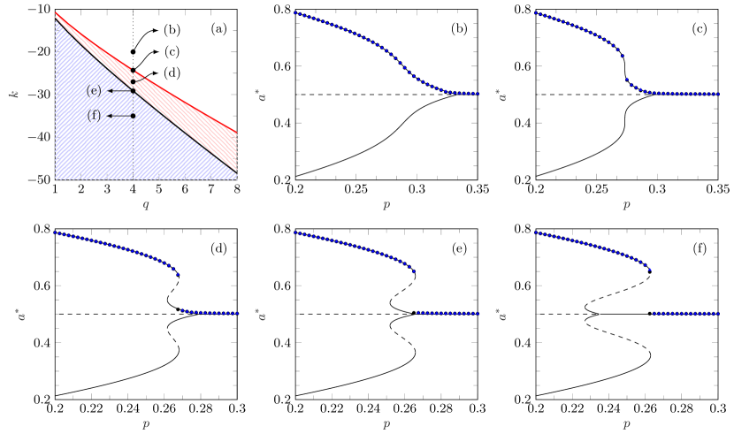
Figure 5: Behavior of the model with symmetric conformity function, where the annealed and quenched dynamics produce the same diagrams. (a) Phase diagram. The blue and the white regions correspond to the zones of the parameter space where transitions between an ordered and a disordered phase are discontinuous or continuous, respectively. The intermediate red region also presents discontinuous transitions but between two ordered phases with different fraction of adopters. The letters indicate the parameter regions of the following fixed-point diagrams (b)-(f), which present stable (solid lines) and unstable (dashed lines) fixed points for the model with $q=4$ and (b) $k=-20$, (c) $k=\widetilde{k}(q=4)\approx-24.3$, (d) $k=-27$, (e) $k=\bar{k}(q=4)\approx-29.1$, (f) $k=-35$. Symbols represent the results from the simulations of the model with $\bullet$ annealed and $\blacktriangle$ quenched dynamics.

B.2 Non-symmetric conformity function

We have chosen

$$f_{S}(x)=x^{q}$$ (56)

as our representative of non-symmetric conformity functions as this form is commonly used in models of opinion dynamics [23] that originate from the nonlinear $q$-voter model [17]. In the case of non-symmetric conformity functions, annealed and quenched dynamics lead to different results. We cover them separately in the next subsections.

B.2.1 Annealed dynamics

The transition rates take the forms:

$$P_{B\rightarrow A} =\bar{p}f_{I}(a)+(1-\bar{p})a^{q},$$ (57)

$$P_{A\rightarrow B} =\bar{p}\left[1-f_{I}(a)\right]+(1-\bar{p})(1-a)^{q},$$ (58)

which results in the following rate equation

$$\frac{da}{dt}=\bar{p}\left[f_{I}(a)-a\right]+(1-\bar{p})\left[(1-a)a^{q}-a(1-a)^{q}\right].$$ (59)

The first group of fixed points is given by $a^{*}=1/2$ and any value of $\bar{p}$, and the second group satisfies the following formula:

$$\bar{p}=\frac{a^{*}(1-a^{*})^{q}-(1-a^{*})(a^{*})^{q}}{a^{*}\left[(a^{*})^{q}+(1-a^{*})^{q}-1\right]+f_{I}(a^{*})-(a^{*})^{q}}.$$ (60)

To check the stability of the derived fixed points, let us denote the right hand side of Eq. (59) by $F(a)$. The stability is determined by the sign of

$$F^{\prime}(a^{*})=\bar{p}\left[f^{\prime}_{I}(a^{*})-1\right]+(1-\bar{p})\left[q(1-a^{*})(a^{*})^{q-1}+qa^{*}(1-a^{*})^{q-1}-(a^{*})^{q}-(1-a^{*})^{q}\right],$$ (61)

where

$$f^{\prime}_{I}(a^{*})=\frac{ke^{-k(a^{*}-a_{0})}}{\left[1+e^{-k(a^{*}-a_{0})}\right]^{2}}.$$ (62)

For $a^{*}=1/2$, we can determine the stability analytically. In this case, we have

$$f^{\prime}_{I}(1/2)=\frac{k}{4},$$ (63)

and

$$F^{\prime}(1/2)=\bar{p}\left[\frac{k}{4}-1\right]+(1-\bar{p})\frac{q-1}{2^{q-1}}.$$ (64)

Consequently, the point at which the stability of $a^{*}=1/2$ changes is given by

$$\bar{p}^{*}=\frac{q-1}{q-1+2^{q-1}\left(1-\frac{k}{4}\right)}.$$ (65)

If $q>1$ and $k<4$, the fixed point $a^{*}=1/2$ is unstable for $\bar{p}<\bar{p}^{*}$, and it is stable for $\bar{p}>\bar{p}^{*}$, whereas if $k>4$, $a^{*}=1/2$ is unstable for all $\bar{p}$. If $0<q<1$ and $k<4$, $a^{*}=1/2$ is stable for all $\bar{p}$, whereas if $k>4$, $a^{*}=1/2$ is stable for $\bar{p}<\bar{p}^{*}$, and it is unstable for $\bar{p}>\bar{p}^{*}$. The stability of the remaining fixed points, given by Eq. (60), is determined numerically.

At the fixed point $(a^{*},\bar{p})=(1/2,\bar{p}^{*})$, a pitchfork bifurcation takes place. This bifurcation changes its type from subcritical to supercritical in the parameter space $(k,q)$ along the curve $k^{*}(q)$ defined by the equation:

$$(k^{*})^{3}+8(k^{*}-4)(q-5)q=0.$$ (66)

The bifurcation is subcritical for $k<k^{*}(q)$, while it becomes supercritical for $k>k^{*}(q)$.

Note that this model for $k=0$ corresponds to the $q$-voter model with independence [26, 31, 27] or the non-linear noisy voter model [25].

B.2.2 Quenched dynamics

In this case, the rate equations have the following forms:

$$\frac{da_{0}}{dt} =(1-a_{0})a^{q}-a_{0}(1-a)^{q},$$ (67)

$$\frac{da_{1}}{dt} =f_{I}(a)-a_{1},$$ (68)

where

$$a=(1-p)a_{0}+pa_{1}.$$ (69)

The first group of fixed points is given by $(a_{0}^{*},a_{1}^{*})=(1/2,1/2)$ and any value of $\bar{p}$, whereas the second group satisfies the following formulas:

$$a_{0}^{*} =\frac{(a^{*})^{q}}{(a^{*})^{q}+(1-a^{*})^{q}},$$ (70)

$$a_{1}^{*} =f_{I}(a^{*}),$$ (71)

where

$$a^{*}=(1-\bar{p})a_{0}^{*}+\bar{p}a_{1}^{*}.$$ (72)

As a result, we have

$$\bar{p}=\frac{a^{*}(1-a^{*})^{q}-(1-a^{*})(a^{*})^{q}}{f_{I}(a^{*})\left[(a^{*})^{q}+(1-a^{*})^{q}\right]-(a^{*})^{q}}.$$ (73)

To check the stability of the derived fixed points, let us denote the right hand side of Eqs. (67) and (68) by $F_{0}(a_{0},a_{1})$ and $F_{1}(a_{0},a_{1})$, respectively. The stability is determined by the use of the Jacobian matrix given by Eq. (44) where

$$\frac{\partial F_{0}}{\partial a_{0}} =q(1-\bar{p})\left[a_{0}(1-a)^{q-1}+(1-a_{0})a^{q-1}\right]-a^{q}-(1-a)^{q},$$ (74)

$$\frac{\partial F_{0}}{\partial a_{1}} =q\bar{p}\left[a_{0}(1-a)^{q-1}+(1-a_{0})a^{q-1}\right],$$ (75)

$$\frac{\partial F_{1}}{\partial a_{0}} =(1-\bar{p})f_{I}^{\prime}(a),$$ (76)

$$\frac{\partial F_{1}}{\partial a_{1}} =\bar{p}f_{I}^{\prime}(a)-1.$$ (77)

For $(a_{0}^{*},a_{1}^{*})=(1/2,1/2)$, we can determine the stability analytically. In this case, we have

$$\left.\frac{\partial F_{0}}{\partial a_{0}}\right|_{(1/2,1/2)} =\frac{1}{2^{q-1}}\left[q(1-\bar{p})-1\right],$$ (78)

$$\left.\frac{\partial F_{0}}{\partial a_{1}}\right|_{(1/2,1/2)} =\frac{1}{2^{q-1}}q\bar{p},$$ (79)

$$\left.\frac{\partial F_{1}}{\partial a_{0}}\right|_{(1/2,1/2)} =\frac{k}{4}(1-\bar{p}),$$ (80)

$$\left.\frac{\partial F_{1}}{\partial a_{1}}\right|_{(1/2,1/2)} =\frac{k}{4}\bar{p}-1.$$ (81)

Thus, the determinant and the trace are the following:

$$\det\left[\mathbf{J}(1/2,1/2)\right] =\frac{1}{2^{q-1}}\left[1-\frac{k}{4}\bar{p}-q(1-\bar{p})\right],$$ (82)

$$\text{tr}\left[\mathbf{J}(1/2,1/2)\right] =\frac{1}{2^{q-1}}\left[q(1-\bar{p})-1\right]+\frac{k}{4}\bar{p}-1.$$ (83)

As a result, the point at which the stability of $(a_{0}^{*},a_{1}^{*})=(1/2,1/2)$ changes is

$$\bar{p}^{*}=\frac{4\left(q-1\right)}{4q-k}.$$ (84)

If $q>1$ and $k<4$, the fixed point $(a_{0}^{*},a_{1}^{*})=(1/2,1/2)$ is unstable for $\bar{p}<\bar{p}^{*}$, and it is stable for $\bar{p}>\bar{p}^{*}$, whereas if $k>4$, $(a_{0}^{*},a_{1}^{*})=(1/2,1/2)$ is unstable for all $\bar{p}$. If $0<q<1$ and $k<4$, $(a_{0}^{*},a_{1}^{*})=(1/2,1/2)$ is stable for all $\bar{p}$, whereas if $k>4$, $(a_{0}^{*},a_{1}^{*})=(1/2,1/2)$ is stable for $\bar{p}<\bar{p}^{*}$, and it is unstable for $\bar{p}>\bar{p}^{*}$. The stability of the remaining fixed points, given by Eq. (73), is determined numerically.

At the fixed point $(a^{*},\bar{p})=(1/2,\bar{p}^{*})$, a pitchfork bifurcation takes place. This bifurcation changes its type from subcritical to supercritical in the parameter space $(k,q)$ along the curve $k^{*}(q)$ defined by the equation:

$$(k^{*})^{3}+16(4-k^{*})(q+1)q=0$$ (85)

The bifurcation is subcritical for $k<k^{*}(q)$, while it becomes supercritical for $k>k^{*}(q)$.

Note that this model for $k=0$ corresponds to the $q$-voter model with independence under the quenched approach from Ref. [27].

B.2.3 Results

Figure 6 illustrates the behavior of the model with the non-symmetric conformity function for (a)-(d) annealed and (e)-(h) quenched dynamics. In the parameter space presented in Fig. 6(a) and 6(e), we can identify two areas separated by the black curve, $k^{*}(q)$, given by Eqs. (66) and (85). For $k>k^{*}(q)$, the system exhibits continuous transitions between a phase where one option dominates over the other (i.e., ordered phase for $\bar{p}<\bar{p}^{*}$) to a phase without the majoritarian option (i.e., disordered phase for $\bar{p}>\bar{p}^{*}$), see Figs. 6(b) and 6(f). At $k^{*}(q)$, the system still exhibits continuous phase transitions, see Figs. 6(c) and 6(g). However, crossing this curve results in a change of the phase transition type. Consequently, for $k<k^{*}(q)$, the transitions between ordered and disordered phases are discontinuous, see Figs. 6(d) and 6(h).

((a))

((b))

((c))

((d))

((e))

((f))

((g))

((h))

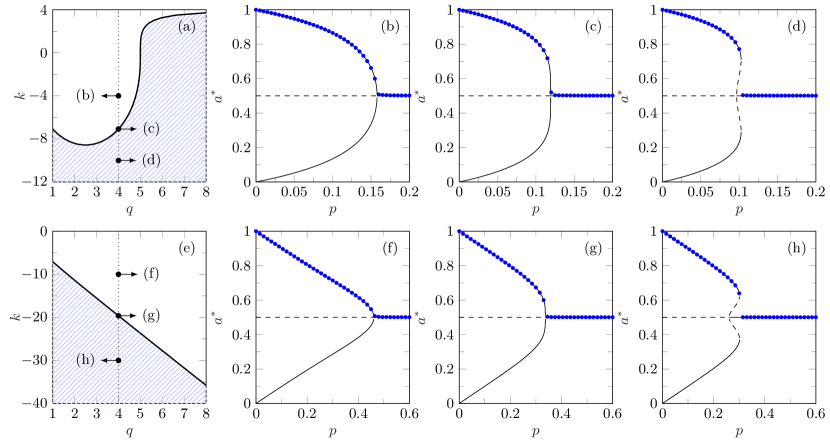
Figure 6: Behavior of the model with non-symmetric conformity function for (a)-(d) annealed and (e)-(h) quenched dynamics. (a) and (e) Phase diagrams. The blue and the white regions correspond to the zones of the parameter space where transitions between an ordered and a disordered phase are discontinuous or continuous, respectively. The letters indicate the parameter regions of the following fixed-point diagrams (b)-(d) and (f)-(h), which present stable (solid lines) and unstable (dashed lines) fixed points for the model with $q=4$ and (b) $k=-4$, (c) $k=k^{*}(q=4)\approx-7.1$, (d) $k=-10$, (f) $k=-10$, (g) $k=k^{*}(q=4)\approx-19.6$, (h) $k=-30$. Symbols represent the results from the simulations of the model.

Appendix C Simulations

C.1 Simulation details

In addition to the analytical results discussed in the main text, which correspond to the thermodynamic limit, we simulate the dynamical equations for a large but finite population of $N=10^{5}$ agents. We consider one time step of this dynamics when $N$ agents have been updated, or in other words when, on average, all the agents have been updated once, in analogy with the notion of Monte Carlo step per site (MCS/s). In the simulations, we trace the fraction of adopters of the most common option, i.e.,

$$\alpha=\max\{a,b\},$$ (86)

where $a$ and $b=1-a$ are the fraction of adopters of the options $A$ and $B$, respectively. In the figures, we show the mean value of $\alpha$, $\left[\langle\alpha\rangle_{t}\right]_{s}$. The angle brackets represent the average over time. We discarded the first 900 MCS to let the system reach the stationary state and perform the time average over next 100 MCS. The square brackets represent the sample average that was performed over 20 independent simulations at most (in a metastable region, the average is perform over those of the simulations that ended up in the same phase). In all the simulations, all the agents are initialized with option $A$. Standard errors are of the mark size order.

When simulating the quenched dynamics, instead of randomly assigning the learning strategies, which would lead to some fluctuations in $\bar{p}$ between simulations, we assign them deterministically. We choose the first $pN$ agents to be individual learners and the rest of them to be social learners. In such a way, we have exactly the same value of $\bar{p}$ in all the simulations that we average over. The problem with the fluctuations can be also overcome by keeping the random assignment but increasing the number of agents in the system as the fluctuations in $\bar{p}$ diminishes with the system size at a rate of $1/\sqrt{N}$.

C.2 Source code

The model is implemented in C++ using object-oriented programming. Python and Matlab are used for data analysis and numerical calculations. The code files can be found in the following GitHub repositories:

• https://github.com/arkadiusz-jedrzejewski/norm-formation-abm,

• https://github.com/arkadiusz-jedrzejewski/norm-formation-abm-py,

• https://github.com/arkadiusz-jedrzejewski/norm-formation-m.

References

- Rendell et al. [2011] L. Rendell, L. Fogarty, W. J. Hoppitt, T. J. Morgan, M. M. Webster, and K. N. Laland, Cognitive culture: theoretical and empirical insights into social learning strategies, Trends Cogn. Sci. 15, 68 (2011).
- Aplin et al. [2014] L. M. Aplin, D. R. Farine, J. Morand-Ferron, A. Cockburn, A. Thornton, and B. C. Sheldon, Experimentally induced innovations lead to persistent culture via conformity in wild birds, Nature 518, 538 (2014).
- Kendal et al. [2018] R. L. Kendal, N. J. Boogert, L. Rendell, K. N. Laland, M. Webster, and P. L. Jones, Social learning strategies: Bridge-building between fields, Trends Cogn. Sci. 22, 651 (2018).
- Whiten and Ham [1992] A. Whiten and R. Ham, On the nature and evolution of imitation in the animal kingdom: Reappraisal of a century of research, Adv. Study Behav. 21, 239 (1992).
- Whiten et al. [2009] A. Whiten, N. McGuigan, S. Marshall-Pescini, and L. M. Hopper, Emulation, imitation, over-imitation and the scope of culture for child and chimpanzee, Philos. Trans. R. Soc. B 364, 2417 (2009).
- Boyd and Richerson [1988] R. Boyd and P. J. Richerson, Culture and the evolutionary process (University of Chicago press, 1988).
- Rogers [1988] A. R. Rogers, Does biology constrain culture, Am. Anthropol. 90, 819 (1988).
- Boyd and Richerson [1995] R. Boyd and P. J. Richerson, Why does culture increase human adaptability?, Ethol. Sociobiol. 16, 125 (1995).
- Enquist et al. [2007] M. Enquist, K. Eriksson, and S. Ghirlanda, Critical social learning: a solution to rogers’s paradox of nonadaptive culture, Am. Anthropol. 109, 727 (2007).
- Ehn and Laland [2012] M. Ehn and K. Laland, Adaptive strategies for cumulative cultural learning, J. Theor. Biol. 301, 103 (2012).
- DiMaggio and Garip [2012] P. DiMaggio and F. Garip, Network effects and social inequality, Annu. Rev. Sociol. 38, 93 (2012).
- Yang et al. [2021] V. C. Yang, M. Galesic, H. McGuinness, and A. Harutyunyan, Dynamical system model predicts when social learners impair collective performance, Proc. Natl. Acad. Sci. U.S.A. 118, e2106292118 (2021).
- McElreath et al. [2008] R. McElreath, A. V. Bell, C. Efferson, M. Lubell, P. J. Richerson, and T. Waring, Beyond existence and aiming outside the laboratory: estimating frequency-dependent and pay-off-biased social learning strategies, Philos. Trans. R. Soc. B 363, 3515 (2008).
- Claidière et al. [2014] N. Claidière, M. Bowler, S. Brookes, R. Brown, and A. Whiten, Frequency of behavior witnessed and conformity in an everyday social context, PLOS ONE 9, 1 (2014).
- Derex et al. [2013] M. Derex, B. Godelle, and M. Raymond, Social learners require process information to outperform individual learners, Evolution 67, 688 (2013).
- Morgan et al. [2012] T. J. H. Morgan, L. E. Rendell, M. Ehn, W. Hoppitt, and K. N. Laland, The evolutionary basis of human social learning, Proc. Royal Soc. B 279, 653 (2012).
- Castellano et al. [2009] C. Castellano, M. A. Muñoz, and R. Pastor-Satorras, Nonlinear -voter model, Phys. Rev. E 80, 041129 (2009).
- Bond et al. [2020] T. Bond, Z. Yan, and M. Heene, Applying the Rasch model: Fundamental measurement in the human sciences (Routledge, 2020).
- Byrka et al. [2016] K. Byrka, A. Jędrzejewski, K. Sznajd-Weron, and R. Weron, Difficulty is critical: The importance of social factors in modeling diffusion of green products and practices, Renew. Sust. Energ. Rev. 62, 723 (2016).
- Kaiser et al. [2010] F. G. Kaiser, K. Byrka, and T. Hartig, Reviving Campbell’s paradigm for attitude research, Pers. Soc. Psychol. Rev. 14, 351 (2010).
- Efferson et al. [2008] C. Efferson, R. Lalive, P. J. Richerson, R. McElreath, and M. Lubell, Conformists and mavericks: the empirics of frequency-dependent cultural transmission, Evol. Hum. Behav. 29, 56 (2008).
- Lumsden and Wilson [1980] C. J. Lumsden and E. O. Wilson, Translation of epigenetic rules of individual behavior into ethnographic patterns, Proc. Natl. Acad. Sci. U.S.A. 77, 4382 (1980).
- Jędrzejewski and Sznajd-Weron [2019] A. Jędrzejewski and K. Sznajd-Weron, Statistical Physics Of Opinion Formation: Is it a SPOOF?, C. R. Phys. 20, 244 (2019).
- Jędrzejewski and Sznajd-Weron [2020] A. Jędrzejewski and K. Sznajd-Weron, Nonlinear -voter model from the quenched perspective, Chaos 30, 013150 (2020).
- Peralta et al. [2018] A. F. Peralta, A. Carro, M. San Miguel, and R. Toral, Analytical and numerical study of the non-linear noisy voter model on complex networks, Chaos 28, 075516 (2018).
- Nyczka et al. [2012] P. Nyczka, K. Sznajd-Weron, and J. Cisło, Phase transitions in the -voter model with two types of stochastic driving, Phys. Rev. E 86, 011105 (2012).
- Jędrzejewski and Sznajd-Weron [2017] A. Jędrzejewski and K. Sznajd-Weron, Person-situation debate revisited: Phase transitions with quenched and annealed disorders, Entropy 19, 415 (2017).
- Morgan and Laland [2012] T. J. H. Morgan and K. N. Laland, The biological bases of conformity, Front. Neurosci. 6, 87 (2012).
- Claidière et al. [2012] N. Claidière, M. Bowler, and A. Whiten, Evidence for weak or linear conformity but not for hyper-conformity in an everyday social learning context, PLOS ONE 7, 1 (2012).
- Strogatz [2015] S. H. Strogatz, Nonlinear dynamics and chaos: with applications to physics, biology, chemistry, and engineering (CRC Press, 2015).
- Nyczka and Sznajd-Weron [2013] P. Nyczka and K. Sznajd-Weron, Anticonformity or independence?—Insights from statistical physics, J. Stat. Phys. 151, 174 (2013).