Enhancing quantum state tomography via resource-efficient attention-based neural networks

Abstract

Resource-efficient quantum state tomography is one of the key ingredients of future quantum technologies. In this work, we propose a new tomography protocol combining standard quantum state reconstruction methods with an attention-based neural network architecture. We show how the proposed protocol is able to improve the averaged fidelity reconstruction over linear inversion and maximum-likelihood estimation in the finite-statistics regime, reducing at least by an order of magnitude the amount of necessary training data. We demonstrate the potential use of our protocol in physically relevant scenarios, in particular, to certify metrological resources in the form of many-body entanglement generated during the spin squeezing protocols. This could be implemented with the current quantum simulator platforms, such as trapped ions, and ultra-cold atoms in optical lattices.

I Introduction

Modern quantum technologies are fuelled by resources such as coherence, quantum entanglement, or Bell nonlocality. Thus, a necessary step to assess the advantage they may provide is the certification of the above features Gühne and Tóth (2009); da Silva et al. (2011); Kliesch and Roth (2021); Tavakoli (2020); Friis et al. (2019); Eisert et al. (2020); Sotnikov et al. (2022); Chen et al. (2022); Gočanin et al. (2022); Boghiu et al. (2023). The resource content of a preparation is revealed from the statistics (e.g. correlations) the device is able to generate. Within the quantum formalism, such data is encoded in the density matrix, which can only be reconstructed based on finite information from experimentally available probes – a process known as quantum state tomography (QST) Leonhardt (1995); White et al. (1999); Roos et al. (2004); Häffner et al. (2005); Gross et al. (2010a); Gross (2011); Tóth et al. (2010a); Moroder et al. (2012); Cramer et al. (2010); Baumgratz et al. (2013); Lanyon et al. (2017). Hence, QST is a prerequisite to any verification task. On the other hand, the second quantum revolution brought new experimental techniques to generate and control massively correlated states in many-body systems Acín et al. (2018); Kinos et al. (2021); Laucht et al. (2021); Becher et al. (2022); Fraxanet et al. (2022), challenging established QST protocols. Both reasons elicited an extremely active field of research that throughout the years offered a plethora of algorithmic techniques Gross et al. (2010b); Flammia et al. (2012); Huszár and Houlsby (2012); Kravtsov et al. (2013); Granade et al. (2017); Tóth et al. (2010b); Schwemmer et al. (2014); Huang et al. (2020); Aaronson (2020); Cattaneo et al. (2023).

Over the recent years, machine learning (ML), artificial neural networks (NN), and deep learning (DL) entered the field of quantum technologies Dawid et al. (2022), offering many new solutions to quantum problems, also in the context of QST Torlai et al. (2018); Carrasquilla et al. (2019); Cha et al. (2021); Melkani et al. (2020); Schmale et al. (2022); Xin et al. (2019). The supervised DL approaches were already successfully tested on experimental data Palmieri et al. (2020); Pan and Zhang (2022); Koutný et al. (2022); Ahmed et al. (2021), wherein a study of neural network quantum states beyond the shot-noise appeared only recently Zhao et al. (2023). Nevertheless, neural network-based methods are not exempted from limitations, i.e. NN can provide non-physical outcomes Carrasquilla and Torlai (2021); Palmieri et al. (2020); Koutný et al. (2022), and are limited in ability to learn from a finite number of samples Westerhout et al. (2020).

In this work, we address the abovementioned drawback by offering a computationally fast general protocol to back up any finite-statistic QST algorithms within a DL-supervised approach, greatly reducing the necessary number of measurements performed on the unknown quantum state. We treat the finite-statistic QST reconstructed density matrix as a noisy version of the target density matrix, and we employ a deep neural network as a denoising filter, which allows us to reconstruct the target density matrix. Furthermore, we connect the mean-squared error loss function with quantum fidelity between the target and the reconstructed state. We show that the proposed protocol greatly reduces the required number of prepared measurements allowing for high-fidelity reconstruction $\sim 98\%$ of both mixed and pure states. We also provide an illustration of the power of our method in, a physically useful, many-body spin-squeezing experimental protocol.

The paper is organized as follows: in Sec. II we introduce the main concepts behind the QST; in Sec. III we introduce the data generation protocol and neural network architecture, as well as define QST as a denoising task. Sec. IV is devoted to benchmarking our method against known approaches, and we test it on quantum states of physical interest. In Sec. V, we provide practical instructions to implement our algorithm in an experimental setting. We conclude in Sec. VI with several future research directions.

II Preliminaries

Let us consider $d$-dimensional Hilbert space. A set of informationally complete (IC) measurement operators $\hat{\bm{\pi}}=\{\hat{\pi}_{i}\}$, $i=1,\dots,d^{2}$, in principle allows to unequivocally reconstruct the underlying target quantum state $\hat{\tau}\in\mathbb{C}^{d\times d}$ in the limit of an infinite number of ideal measurements Fuchs and Schack (2013); Fuchs et al. (2017). After infinitely many measurements, one can infer the mean values:

$$p_{i}=\mathrm{Tr}[\hat{\tau}\hat{\pi}_{i}],$$ (1)

and construct a valid vector of probabilities $\mathbf{p}=\{p_{i}\}$ for any proper state $\hat{\tau}\in\mathcal{S}$, whereby $\mathcal{S}$ we denote the set of $d$-dimensional quantum states, i.e. containing all unit-trace, positive semi-definite (PSD) $d\times d$ Hermitian matrices. Moreover, $\hat{\bm{\pi}}$ can be considered as a set of operators spanning the space of Hermitian matrices. In such a case, $\mathbf{p}$ can be evaluated from multiple measurement settings (e.g., Pauli basis) and is generally no longer a probability distribution. In any case, there exists a one-to-one mapping $Q$ from the mean values $\mathbf{p}$ to the target density matrix $\hat{\tau}$:

$$Q: \mathcal{F}_{\mathcal{S}}\longrightarrow\mathcal{S}$$ (2)

$$\mathbf{p}\longmapsto Q[\mathbf{p}]=\hat{\tau},$$

where $\mathcal{F}_{\mathcal{S}}$ is the space of accessible probability vectors. In particular, by inverting the Born’s rule Eq. (1), elementary linear algebra allows us to describe the map $Q$ as,

$$Q[\mathbf{p}]=\mathbf{p}^{T}\mathrm{Tr}[\hat{\bm{\pi}}\hat{\bm{\pi}}^{T}]^{-1}\hat{\bm{\pi}}.$$ (3)

The inference of the mean values $\mathbf{p}$ is only perfect in the limit of an infinite number of measurement shots, $N\rightarrow\infty$.

In a realistic scenario, with a finite number of experimental runs $N$, we have access to frequencies of relative occurrence $\mathbf{f}=\{f_{i}:=n_{i}/N\}$, where $n_{i}$ is the number of times the outcome $i$ is observed. Such counts allow us to estimate $\mathbf{p}$ within an unavoidable error dictated by the shot noise and of amplitude typically scaling as $1/\sqrt{N}$ Peter and Petrosyan (2007). With only the frequencies $\mathbf{f}$ available, we can use the mapping $Q$ for an estimate $\hat{\rho}$ of the target density matrix $\hat{\tau}$, i.e.,

$$\hat{\rho}=Q[\mathbf{f}],$$ (4)

In the infinite number of trials $N\to\infty$, $f_{i}=p_{i}$ and $\hat{\rho}=\hat{\tau}$. Yet, in the finite statistics regime, as considered in this work, the application of the mapping as defined in Eq. (3) to the frequency vector $\mathbf{f}$ will generally lead to nonphysical results (i.e. $\hat{\rho}$ not PSD). In such case, as an example of proper mapping $Q$, we can consider different methods for standard tomography tasks, such as Linear Inversion (LI), or Maximum Likelihood Estimation (MLE), see Appendix A. As operators $\bm{\hat{\pi}}$, we consider positive operator-valued measures (POVMs) and the more experimentally appealing Pauli basis (check Appendix B).

III Methods

This section describes our density matrix reconstruction protocol, data generation, neural network (NN) training, and inference procedure. In Fig. 1, we show how such elements interact within the data flow. In the following paragraphs, we elaborate on the proposed protocol in detail.

The first step in our density matrix reconstruction protocol, called pre-processing, is a reconstruction of density matrix $\hat{\rho}$ via finite-statistic QST with frequencies $\mathbf{f}$ obtained from measurement prepared on target state $\hat{\tau}$. Next, we feed forward the reconstructed density matrix $\hat{\rho}$ through our neural network acting as a noise filter – we call this stage a post-processing. In order to enforce the positivity of the neural network output, we employ the so-called Cholesky decomposition to the density matrices, i.e. $\hat{\rho}=C_{\rho}C_{\rho}^{\dagger}$, and $\hat{\tau}=C_{\tau}C_{\tau}^{\dagger}$, where $C_{\rho,\tau}$ are lower-triangular matrices. Such decomposition is unique, provided that $\hat{\rho}$, $\hat{\tau}$ is positive . We treat the Cholesky matrix $C_{\rho}$ obtained from finite-statistic QST protocol, as a noisy version of the target Cholesky matrix $C_{\tau}$ computed from $\hat{\tau}$. The aim of the proposed neural network architecture is to learn a denoising filter allowing reconstruction of the target $C_{\tau}$ from the noisy matrix $C_{\rho}$ obtained via finite-statistic QST. Hence, we cast the neural network training process as a supervised denoising task.

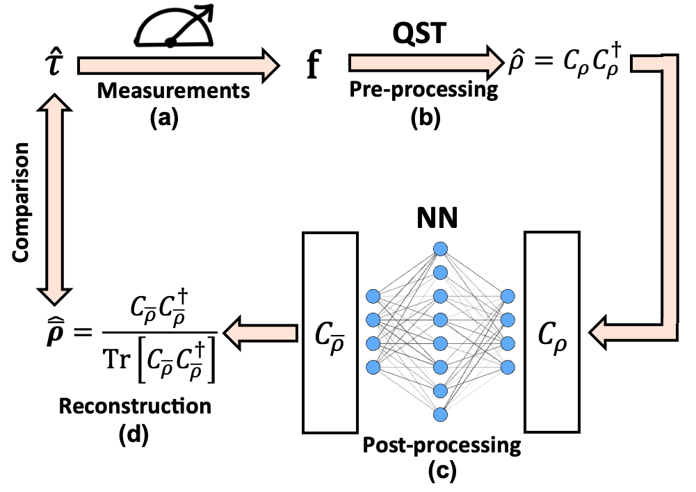
Figure 1: Schematic representation of the data pipeline of our QST hybrid protocol. Panel (a) shows data acquisition from a generic experimental set-up, during which the frequencies $\mathbf{f}$ are collected. Next, panel (b) presents standard density matrix reconstruction; in our work, we test the computationally cheap LI method together with the expensive MLE, in order to better analyse the network reconstruction behaviour and ability. Panel (c) depicts the matrix-to-matrix deep-learning strategy for Cholesky matrices reconstruction. The architecture herein considered is a combination of convolutional layers for input and output and a transformer model in between. Finally, we compare the reconstructed state $\hat{\bar{\rho}}$ with the target $\hat{\tau}$.

III.1 Training data generation

To construct the training data set, we first start with generating $N_{\rm train}$ Haar-random $d$-dimensional target density matrices, $\{\hat{\tau}_{m}\}$, where $m=1,\dots,N_{\rm train}$. Next, we simulate experimental measurement outcomes $\mathbf{f}_{m}$, for each $\hat{\tau}_{m}$, in one of the two ways:

1. Directly : When the measurement operators $\hat{\bm{\pi}}$ form an IC-POVM, we can take into account the noise by simply simulating the experiment and extracting the corresponding frequency vector $\mathbf{f}_{m}=\{n_{i}/N\}_{m}$, where $N$ is the total number of shots (i.i.d. trials) and the counts $\{n_{i}\}_{m}$ are sampled from the multinomial distribution.

2. Indirectly : As introduced in the preliminaries (Sec. II), if a generic basis is used $\hat{\bm{\pi}}$, $\mathbf{p}_{m}$ is no longer necessarily a probability distribution. This is the case with the Pauli basis (as defined in Appendix B), that we exploit in our examples. Then, we can add a similar amount of noise, obtaining $\mathbf{f}_{m}=\mathbf{p}_{m}+\delta\mathbf{p}_{m}$, where $\delta\mathbf{p}_{m}$ is sampled from the multi-normal distribution $\mathcal{N}(\mathbf{0},\sim\mathbb{1}/(2\sqrt{N}))$ of mean zero and isotropic variance, saturating the shot noise limit.

Having prepared frequency vectors $\{\mathbf{f}_{m}\}$, we apply QST via mapping $Q$, Eq. (4), obtaining set of reconstructed density matrices $\{\hat{\rho}_{m}\}$. We employ the most rudimentary and scalable method, i.e. the linear inversion QST, however, other QST methods can be utilized as well. Finally, we construct the training dataset as $N_{\rm train}$ pairs $\big{\{}\vec{C}_{\rho},\vec{C}_{\tau}\big{\}}$, where we use $\vec{C}$ to indicate the vectorization (flattening) of the Cholesky matrix $C$ (see Appendix C for definition).

III.2 Neural network training

The considered neural network, working as a denoising filter, is a non-linear function $h_{\bm{\theta}}$ preparing matrix-to-matrix mapping, in its vectorized form, $h_{\bm{\theta}}:\vec{C}_{\rho}\to\vec{C}_{\bm{\theta}}$, where $\bm{\theta}$ incorporates all the variational parameters such as weights and biases to be optimized. The neural network training process relies on minimizing the cost function defined as a mean-squared error (MSE) of the network output with respect to the (vectorization of) target density matrix $\hat{\tau}$, i.e.

$${\cal L}^{\rm MSE}(\bm{\theta})=\|\vec{C}_{\tau}-\vec{C}_{\bm{\theta}}\|^{2},$$ (5)

via the presentation of $K$ training samples $\{\hat{\rho}_{l}\}_{l=1}^{K}$. The equivalence between MSE and Hilbert-Schmidt (HS) distance is discussed in detail in Appendix C, where we also demonstrate that the mean-squared error used in the cost function, Eq. (5), is a natural upper bound of the quantum fidelity. Hence, the choice of the cost function, Eq. (5), not only is the standard cost function for the neural network but also approximates the target state in a proper quantum metric. To make the model’s optimization more efficient and avoid overfitting, we add a regularizing term resulting in the total cost function ${\cal L}^{\rm MSE}(\bm{\theta})+\mathrm{Tr}[C_{\bm{\theta}}C_{\bm{\theta}}^{\dagger}]$ (chapter 7 of Ref. Goodfellow et al. (2016)).

The training process results in an optimal set of parameters of the neural network $\bar{\bm{\theta}}=\text{arg min}_{\bm{\theta}}{\cal L}$, and trained neural network $h_{\bar{\bm{\theta}}}$, which allows for the reconstruction of the target density matrix $\hat{\tau}$ via Cholesky matrix $C_{\bar{\rho}}$ , i.e.

$$\hat{\bar{\rho}}=\frac{C_{\bar{\rho}}C_{\bar{\rho}}^{\dagger}}{\Tr[C_{\bar{\rho}}C_{\bar{\rho}}^{\dagger}]}\simeq\hat{\tau},$$ (6)

where $C_{\bar{\rho}}$ is reshaped from $\vec{C}_{\bar{\rho}}=h_{\bar{\bm{\theta}}}(\vec{C}_{\rho})$.

III.3 Neural network architecture

Our proposed architecture gets inspiration from the other recent models Zhu et al. (2022); Requena et al. (2023), combining convolutional layers with a transformer layer implementing a self-attention mechanism Bahdanau et al. (2016); Vaswani et al. (2023). A convolutional neural network extracts important features from the input data, while a transformer block distils correlations between features via the self-attention mechanism. The self-attention mechanism utilizes the representation of the input data as nodes inside a graph Dwivedi and Bresson (2021) and aggregates relations between the nodes.

The architecture of considered neural network $h_{\bm{\theta}}$ contains two convolutional layers $h_{\mathrm{cnn}}$ and transformer layer $h_{\mathrm{tr}}$ in between, i.e.:

$$h_{\bm{\theta}}(\vec{C}_{\rho})=\mathrm{tanh}[h_{\mathrm{\mathrm{cnn}}}\circ h_{\mathrm{tr}}\circ\gamma(h_{\mathrm{\mathrm{cnn}}})](\vec{C}_{\rho}),$$ (7)

where $\gamma(y)=1/2y(1+\text{Erf}(y)/\sqrt{2})$, $y\in\mathbb{R}$, is the Gaussian Error Linear Unit (GELU) activation function Hendrycks and Gimpel (2023) broadly used in the modern transformers architectures, and $\tanh(y)$ is the hyperbolic tangent, acting element-wise of NN nodes.

The first layer $h_{\mathrm{cnn}}$ applies a set of $K$ fixed-size trainable one-dimensional convolutional kernels to $\vec{C}_{\rho}$ followed by non-linear activation function, i.e. $\gamma(h_{\mathrm{cnn}}(\vec{C}_{\rho}))\to\{\bm{F}^{1}_{\mathrm{cnn}},\dots,\bm{F}^{K}_{\mathrm{cnn}}\}$. During the training process, convolutional kernels learn distinct features of the dataset, which are next feedforwarded to the transformer block $h_{\rm tr}$. The transformer block $h_{\rm tr}$ distills the correlations between the extracted features from kernels via the self-attention mechanism, providing a new set of vectors, i.e. $h_{\rm tr}(\bm{F}^{1}_{\mathrm{cnn}},\dots,\bm{F}^{K}_{\mathrm{cnn}})\to\{\bm{F}^{1}_{\mathrm{tr}},\dots,\bm{F}^{K}_{\mathrm{tr}}\}$. The last convolutional layer $h_{\mathrm{cnn}}$ provides an output $\vec{C}_{\bm{\theta}}$, $\mathrm{tanh}(h_{\mathrm{cnn}}(\bm{F}^{1}_{\rm tr},\dots,\bm{F}^{K}_{\rm tr}))\to\vec{C}_{\bm{\theta}}$, where all filter outputs from the last layer are added. Finally, we reshape the output into the lower-triangular form and reconstruct the density matrix via Eq. (6).

The training data and the considered architecture allow interpretation of the trained NN as a conditional debiaser (for details see Appendix D). The proposed protocol cannot improve the predictions of unbiased estimators, however, any estimator that outputs valid quantum states (e.g., LI, MLE) must be biased due to boundary effects. In the given framework, the task of the NN is to learn such skewness and drift the distribution towards the true mean.

IV Results and discussion

Having introduced the features of our NN-based QST enhancer in the previous section, here, we demonstrate its advantages in scenarios of physical interest. To this aim, we consider two examples.

As the first example, we consider an idealized random quantum emitter (see e.g. Refs. Liu et al. (2023); Tang et al. (2022) for recent experimental proposals) that samples high-dimensional mixed states from the Hilbert-Schmidt distribution. After probing the system via single-setting square-root POVM, we are able to show the usefulness of our NN upon improving LI and MLE preprocessed states. We evaluate the generic performance of our solution and compare it with recent proposals of NN-based QST, Ref. Koutný et al. (2022).

In the second example, we focus on a specific class of muti-qubit pure states of special physical relevance, i.e. with metrological potential as quantified by the quantum Fisher information (QFI). Such states are generated via the famous one-axis twisting dynamics Kitagawa and Ueda (1993a); Wineland et al. (1994a). Here, the system is measured using operators $\hat{\bm{\pi}}$ via local symmetric, informationally complete, positive operator-valued measures (SIC-POVM) or experimentally relevant the Pauli operators.

In the following, we discuss the two abovementioned scenarios.

IV.1 Reconstructing high-dimensional random quantum states

Scenario.– As a first illustration, we consider a set of $N_{\rm trial}$ random trial states $\{\hat{\tau}_{j}\}$, $j=1,\dots,N_{\rm train}$ with Hilbert space dimension $d=9$ sampled from the HS distribution (see Appendix E). The first task consists of assessing the average quality reconstruction over such an ensemble to benchmark the generic performance of our NN.

We prepare measurements on each trial state $\hat{\tau}_{j}$ via informationally complete (IC) square-root POVMs as defined in Eq. (15), and obtain state reconstruction $\hat{\bar{\rho}}_{j}$ via two standard QST protocols, i.e. bare LI and MLE algorithms, as well as by our neural network enhanced protocols denoted as LI-NN, and MLE-NN, see Fig. 1. Finally, we evaluate the quality of the reconstruction as the average of the square of the Hilbert-Schmidt distance

$$D_{\rm HS}^{2}(\hat{\bar{\rho}}_{j},\hat{\tau}_{j})=\mathrm{Tr}[(\hat{\bar{\rho}}_{j}-\hat{\tau}_{j})^{2}].$$ (8)

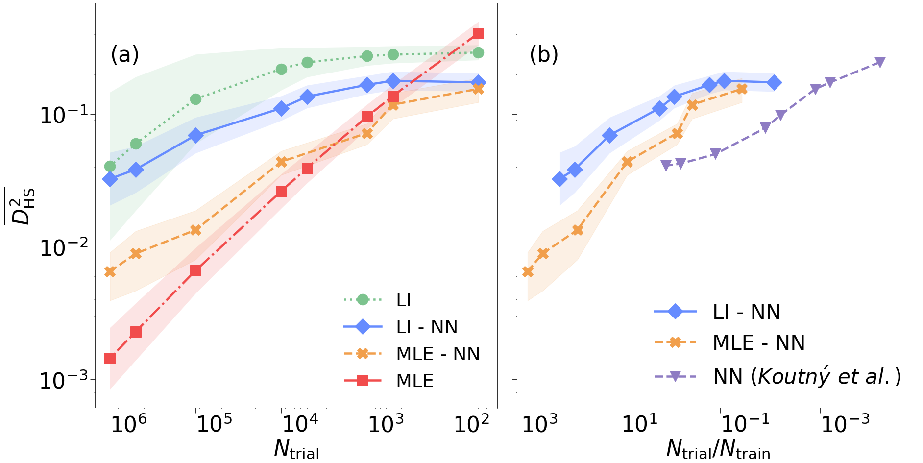
Figure 2: Evaluation of the QST reconstruction measured by the mean value of the Hilber-Schmidt distance square, $\overline{D^{2}}_{\rm HS}$, for different QST protocols, averaged over $N_{\rm test}=1000$ target states. Panel (a) shows mean $D_{\rm HS}^{2}$ for four QST protocols: LI (green dots), MLE (red squares), NN-enhanced LI (blue diamonds), and NN-enhanced MLE (orange crosses). Panel (b) shows $\overline{D^{2}}_{\rm HS}$ as a function of ratio $N_{\rm trial}/N_{\rm train}$ for our LI-NN model (blue squares), MLE-NN model (orange crosses), and for the network model proposed in Ref. Koutný et al. (2022) (violet triangles). A lower number $N_{\rm train}$ shifts lines to the left, indicating resource efficiency. Our proposed protocol achieves competitive averaged HS reconstruction for the size of training data of an order of magnitude smaller compared to the method proposed in Ref. Koutný et al. (2022) (note $x$-axis values increase to the left). During models’ training, we set $N_{\rm train}=1250$ for MLE-NN protocol, and $N_{\rm train}=5000$ for the LI-NN. Lines are to guide the eye, shadow areas represent one standard deviation.

Benchmarking.– Fig. 2(a) presents averaged HS distance square $\overline{D^{2}}_{\rm HS}$ as a function of the number of trials states $N_{\rm trial}$, obtained with bare LI, MLE algorithms, and neural network enhanced LI (LI-NN), and neural network enhanced MLE (MLE-NN). The training dataset contains $N_{\rm train}=1250$ HS distributed mixed states. Our neural network-enhanced protocol improves over the LI, and MLE, i.e. $\overline{D^{2}}_{\rm HS}$ is lower for LI-NN, and MLE-NN compared to LI and MLE algorithms for the same $N_{\rm trial}$. For fewer trials $N_{\rm trial}<10^{3}$, the post-processing marginally improves over the states reconstructed only from MLE. For a larger number of trials, the lowest $\overline{D^{2}}_{\rm HS}$ is obtained for MLE results, performing better than other considered tomographic methods. To enhance MLE in the regime of a few samples, we propose an alternative method by incorporating, as a depolarization channel, the statistical noise (see Appendix F).

Next, Fig. 2(b) presents comparison between our protocol with the state-of-the-art density matrix reconstruction via neural network, Ref. Koutný et al. (2022), where the authors report better performance than the MLE and LI algorithms having $N_{\rm train}=8\cdot 10^{5}$ training samples, for states belonging to a Hilbert space of dimension $d\geq 3$. Fig. 2(b) presents $\overline{D^{2}}_{\rm HS}$ as a function of $N_{\rm trial}/N_{\rm train}$, where $N_{\rm train}=1250$ for MLE-NN, and $N_{\rm train}=5000$ for LI-NN. The advantage of our protocol lies in the fact, that the amount of the necessary training data is significantly smaller compared to the training data size in Ref. Koutný et al. (2022), in order to obtain similar reconstruction quality, which is visible as a shift of the lines towards higher values of $N_{\rm trial}/N_{\rm train}$.

IV.2 Certifying metrologically useful entanglement depth in many-body states

Scenario.– In the last experiment, we reconstruct a class of physically relevant multi-qubit pure states. Specifically, we consider a chain of $L=4$ spins-$1/2$ (Hilbert space of dimension $d=16$). The target quantum states are dynamically generated during the one-axis twisting (OAT) protocol Kitagawa and Ueda (1993a); Wineland et al. (1994a)

$$\ket{\Psi(t)}=e^{-it\hat{J}_{z}^{2}}\ket{+}^{\otimes L}\ ,$$ (9)

where $\hat{J}_{z}$ is the collective spin operator along $z$-axis and $\ket{+}^{\otimes L}=[(\ket{\uparrow}+\ket{\downarrow})/\sqrt{2}]^{\otimes L}$ is the initial state prepared in a coherent spin state along $x$-axis (orthogonal to $z$). The OAT protocol generates spin-squeezed states useful for high-precision metrology, allowing to overcome the shot-noise limit Pezzè et al. (2018); Wolfgramm et al. (2010); Wineland et al. (1994b); Müller-Rigat et al. (2023), as well as many-body entangled and the many-body Bell correlated states Tura et al. (2014); Schmied et al. (2016); Aloy et al. (2019); Baccari et al. (2019); Tura et al. (2019); Müller-Rigat et al. (2021); Żukowski and Brukner (2002); Cavalcanti et al. (2007); He et al. (2011); Cavalcanti et al. (2011); Niezgoda et al. (2020); Niezgoda and Chwedeńczuk (2021); Chwedeńczuk (2022); Müller-Rigat et al. (2021). OAT states have been extensively studied theoretically Wineland et al. (1992); Kitagawa and Ueda (1993b); Gietka et al. (2015); Li et al. (2008, 2009); Wang et al. (2017); Kajtoch et al. (2018a); Schulte et al. (2020); Gietka et al. (2021); Comparin et al. (2022), and can be realized with a variety of ultra-cold systems, utilizing atom-atom collisions Riedel et al. (2010); Gross et al. (2010c); Hamley et al. (2012); Qu et al. (2020), and atom-light interactions Leroux et al. (2010); Maussang et al. (2010). The recent theoretical proposals for the OAT simulation with ultra-cold atoms in optical lattices effectively simulate Hubbard and Heisenberg models Kajtoch et al. (2018b); He et al. (2019); Płodzień et al. (2020, 2022, 2023); Mamaev et al. (2021); Hernández Yanes et al. (2022); Dziurawiec et al. (2023); Hernández Yanes et al. (2023).

Preliminary results.– For the first task, we generate our data for testing and training with SIC-POVM operators. For the test set, we select 100 OAT states in evenly spaced times $t\in(0,\pi)$ and assess the average reconstruction achieved by our trained NN on a training dataset with $N_{\rm train}=10,500$ Haar random pure states. We compare the values with the average score obtained for generic Haar distributed states, which is the set the model was trained on (see Appendix E).

	$10^{5}$ trials	$10^{4}$ trials	$10^{3}$ trials
LI-OAT	$94.3\pm 0.4\%$	$86.5\pm 0.1\%$	$67.0\pm 2.0\%$
NN-OAT	$98.6\pm 0.2\%$	$97.8\pm 0.5\%$	$87.6\pm 4.5\%$
NN-Haar	$96.9\pm 3.0\%$	$94.2\pm 3.3\%$	$81.1\pm 4.1\%$

Table 1: Comparison of average fidelity and its standard deviation between the reconstructed and the target states of size $d=16$ for various QST methods (rows), with varying size of measurement trials $N_{\rm trial}=10^{5},10^{4},10^{3}$, as indicated by the consecutive columns. The first row presents the average fidelity reconstruction for linear inversion QST, averaged over OAT states, evenly sampled from $t=0$ to $t=\pi$. Employing our neural network presents an enhancement over the bare LI, as shown in the second row for the same target set. Finally, the third row also shows data for NN-enhanced LI, but averaged over general Haar-random states. All the initial Born values are calculated by noiseless SIC-POVM.

The qualities of reconstructions are shown in Table 1. First, we verify that the NN is able to improve substantially the OAT states, even though no examples of such a class of states were given in the training phase, which relied only on Haar-random states. Moreover, the OAT-averaged reconstruction values exceed the Haar reconstruction ones. We conjecture that this stems from the bosonic symmetry exhibited by the OAT states. This symmetry introduces redundancies in the density matrix which might help the NN to detect errors produced by the statistical noise. Finally, let us highlight that the network also displays good robustness to noise. Indeed, when we feed the same network with states prepared for $N_{\rm trial}=10^{3}$ trials, we increase the reconstruction fidelity moving to $87\%$ from $67\%$.

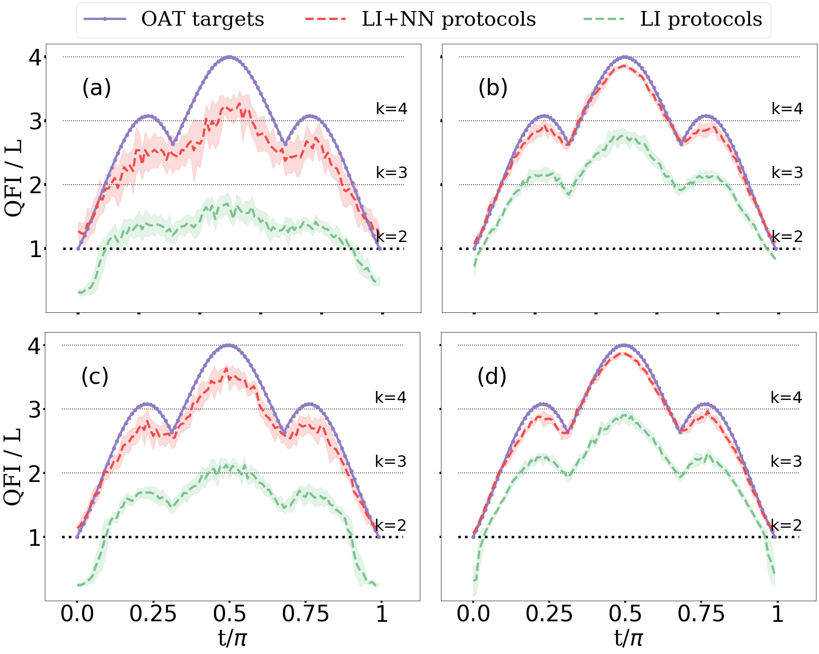
Figure 3: Time evolution of the normalized QFI during the OAT protocol for $L=4$ qubits system. Solid blue lines represent QFI calculated for target quantum states. The mean values of QFI calculated from tomographically reconstructed density matrices are denoted by green-dashed (reconstruction via LI), and red-dotted lines (reconstruction via neural network post-processed LI outputs). Shaded areas mark one standard deviation after averaging over $10$ reconstructions. Panels (a) and (b) correspond to LI protocol with SIC-POVM data, whereas (c) and (d) denote LI reconstruction inferred from Pauli measurements. In the upper row, the left (right) column corresponds to $N_{\rm trial}=10^{3}$ ($10^{4}$) trials; in the lower row, the left (right) column reproduces an LI initial fidelity reconstruction of $\sim 74\%(\sim 86\%)$. The red lines represent the whole setup with NN post-processing of data from corresponding green lines, indicating improvement over the bare LI method. The NN advantage over the bare LI method can be characterized by entanglement depth certification, as shown by the horizontal lines denoting the entanglement depth bounds ranging from the separable limit (bottom line, bold), to the genuine $L$-body limit (top line). In particular, the presence of entanglement is witnessed by $\mathrm{QFI}>L$, as shown by the violation of the separable bound (bold horizontal line).

Inferring the quantum Fisher information (QFI).– Finally, we evaluate the metrological usefulness of the reconstructed states as measured by the quantum Fisher information, $F_{Q}[\hat{\rho},\hat{G}]$. The QFI is a nonlinear function of the state and quantifies the sensitivity upon rotations generated by $\hat{G}$. For more details, we refer the reader to Appendix G.

Here, we use the collective spin component $\hat{J}_{\mathbf{v}}$ as the generator $\hat{G}=\hat{J}_{\mathbf{v}}$, where the orientation $\bm{v}\in\mathbb{S}^{2}$ is chosen so that it delivers the maximal sensitivity. The QFI with respect to collective rotations can also be used to certify quantum entanglement Müller-Rigat et al. (2023), in particular, the entanglement depth $k$, which is the minimal number of genuinely entangled particles that are necessary to describe the many-body state. If $F_{Q}[\hat{\rho},\hat{J}_{\mathbf{v}}]>kL$, then, the quantum state $\hat{\rho}$ has at least $k+1$ entanglement depth Hyllus et al. (2012); Tóth (2012). In particular, for states with depth $k=1$ (i.e., separable), due to the lack of entanglement detected, the metrological power is at most the shot-noise limit Pezzé and Smerzi (2009). This bound is saturated by coherent spin states – like our initial ($t=0$) state for OAT evolution, $\ket{+}^{\otimes L}$.

In Fig. 3, we present the evolution of the QFI (normalized by the coherent limit, $L=4$) for the OAT target states (top solid blue lines). The top row corresponds to SIC-POVM measurement operators $\bm{\hat{\pi}}$, while the bottom row corresponds to projective measurements with Pauli operators. In all experiments, we use the same neural network previously trained on random Haar states with frequencies $\{\mathbf{f}_{m}\}$ obtained from $N_{\rm trial}=10^{4}$ measurement trials. The LI algorithm by itself shows entanglement ($\mathrm{QFI}>L$) for a few times $t$. By enhancing the LI algorithm via our NN protocol, we surpass the three-body bound ($\mathrm{QFI}/L=3$), thus revealing genuine 4-body entanglement, which is the highest depth possible in this system (as it is of size $L=4$). For instance, let us note that at time $t=\pi/2$, the OAT dynamic generates the cat state, $|\Psi(t=\pi/2)\rangle=(e^{-i\pi/4}|+\rangle^{\otimes 4}+e^{+i\pi/4}|-\rangle^{\otimes 4})/\sqrt{2}$, which is genuinely $L$-body entangled, and so it is certified.

IV.3 Discussion

Currently, existing algorithms for QST tend to suffer from either of two main problems: unphysicality of results or biasedness. We tackle the problem of increasing the quality of state reconstruction by enhancing any biased QST estimator with an attention-based neural network working as a denoising filter, see Figure 1. Such an approach corrects both unphysicality and bias, at least partially. Our NN architecture is based on convolutional layers extracting crucial features from input data, and attention-based layers distilling correlations between extracted features. This choice of architecture is motivated by its improved generalization ability enabling a significant reduction of the necessary amount of training data, compared to NN-based approaches not utilizing an attention mechanism. From the examples provided in this section, we infer that our NN-enhanced protocol outperforms other methods of QST in the domain of a small number of measurement samples, see Figure 2. This is especially important due to applications in realistic scenarios, where the trade-off between accuracy and resource cost is crucial.

The results presented in this contribution prove that, with the small number of samples, the comparison of neural network enhancement to pure linear inversion protocol favors our implementation, as can be deduced by fidelity of reconstruction in Table 1. Although the NN was trained on Haar-random pure states, it achieves even better performance on its subset of measure zero, namely one-axis twisted states. We conjecture that this is due to their underlying symmetries, which allows to efficiently learn and correct the noise pattern.

Furthermore, the metrological usefulness of our method is visible through its certification of quantum Fisher information and entanglement depth, see Fig. 3. The bare QST setup, without our NN post-processing, is not able to show entanglement ($\mathrm{QFI}>L$) at any finite time, as well as it never certifies the full genuine $4$-body entanglement. Both of these problems are dealt with by the action of NN-enhancement.

V Concrete experimental implementation for quantum state verification

To recapitulate this contribution, as a complement to Fig. 1 and our repository provided in Ref. Macarone-Palmieri (2023), we summarize the practical implementation of the protocol introduced in this work.

1. Scenario: We consider a finite-dimensional quantum system prepared in a target state $\hat{\tau}$. Here, we aim to verify the preparation of a quantum state $\hat{\tau}$ via QST. To this end, we set a particular measurement basis $\hat{\bm{\pi}}$ to probe the system.

2. Experiment: After a finite number of experimental runs, from the countings, we construct the frequency vector $\mathbf{f}$.

3. Preprocessed quantum state tomography: From the frequency vector $\mathbf{f}$ and the basis $\hat{\bm{\pi}}$, we infer the first approximation of the state $\hat{\rho}$ via the desired QST protocol (e.g., one of those introduced in Appendix A).

4. Assessing pre-reconstruction: We evaluate the quality of the reconstruction by e.g., computing $D^{2}_{\mathrm{HS}}(\hat{\tau},\hat{\rho})$, quantum fidelity or any other meaningful quantum metric. To improve such a score, we resort to our NN solution to complete a denoising task. As with any deep-learning method, training is required.

5. Training neural network: Different training strategies can be implemented:

   1. Train over uniform ensembles (e.g., Haar, HS, Bures etc.) if $\hat{\tau}$ is a typical state or we do not have information about it. If we know certain properties of the target state, we can take advantage of it (see next items).

   2. Train over a subspace of states of interest. For example, if we reconstruct OAT states (Section IVb), we may train only on the permutation-invariant sector.

   3. Train with experimental data. For example, if we have a quantum random source to characterize (Section IVa), experimental data can be used in the training set Palmieri et al. (2020). In such a case, our demonstrated reduction of the training set size translates also to a reduction of the experimental effort.

6. Feeding the neural network: We feed-forward the preprocessed state $\hat{\rho}$ in our trained matrix-to-matrix NN to recover the enhanced quantum state $\hat{\bar{\rho}}$.

7. Assessing the neural network: We compute the updated reconstruction metric on the post-processed state $D^{2}_{\mathrm{HS}}(\hat{\tau},\hat{\bar{\rho}})$. Finally, we assess the usefulness of the NN by comparing how smaller such value is compared to the pre-processed score $D^{2}_{\mathrm{HS}}(\hat{\tau},\hat{\rho})$.

The strength of our proposed protocol lies in its broad applicability, as the choice of the basis $\hat{\bm{\pi}}$ and QST pre-processing method is arbitrary.

VI Conclusions

We proposed a novel deep learning protocol improving standard finite-statistic quantum state tomography methods, such as Linear Inversion and Maximum Likelihood Estimation. Our network, based on the attention mechanism and convolutional layers, greatly reduces the number of required measurements, serving as a denoising filter to the standard tomography output. The versatility of our approach comes from the fact that the measurement basis and reconstruction method have only an implicit impact as our central algorithm works directly with the density matrix. The proposed method reduces the number of necessary measurements on the target density matrix by at least an order of magnitude, compared to DL-QST protocols finite-statistic methods.

We verified that our proposed method is able to improve over LI and MLE preprocessed states. Moreover, the inference stage was performed on out-of-distribution data, i.e., we tested our model on density matrices forming an infinitesimally small fraction of the training dataset, indicating the robustness of the proposed method. In particular, we test our model on $4$-qubits spin-squeezed, and many-body Bell correlated states, generated during one-axis twisting protocol, with average fidelity $\sim 98\%$. We demonstrated our NN improves the reconstruction of a class of physically relevant multi-qubit states, paving the way to use such novel methods in current quantum computers and quantum simulators based on spin arrays.

Our protocol can greatly advance other QST methods, for both arbitrary states as well as for special classes that scale reasonably with the number of particles, such as symmetric states Tóth et al. (2010); Oszmaniec et al. (2016).

Data and code availability.– Data and code are available at Ref. Macarone-Palmieri (2023).

Appendix A Established approaches for state tomography

We review four of the most well-known approaches to quantum state reconstruction that could be potentially improved with the novel protocol proposed in this work.

Linear inversion (LI).– By inverting Born’s rule Eq. (1) (main text) we can express the state dependence on the mean values $\mathbf{p}=\{p_{i}\}$.

$$\hat{\tau}=\mathbf{p}^{T}\mathrm{Tr}[\hat{\bm{\pi}}\hat{\bm{\pi}}^{T}]^{-1}\hat{\bm{\pi}}\ .$$ (10)

Note that the inverse of the Gram matrix $\mathrm{Tr}(\hat{\bm{\pi}}\hat{\bm{\pi}}^{T})$ exists as the basis is informationally-complete (IC). If it is (informationally-) overcomplete, one just needs to replace the inverse with the pseudoinverse. Finally, if it is under-complete (only partial information is available), it will determine the state up to a linear subspace.

The LI method infers $\hat{\rho}$ by replacing in Eq. (10) the ideal expectation values $\mathbf{p}$ with the vector $\mathbf{f}$ of experimental frequencies (counts). This naive substitution generally leads to a negative matrix, $\hat{\rho}\nsucceq 0$. An optimal way to tame its negative eigenvalues was given in Ref. Smolin et al. (2012) by finding the nearest physical state to $\hat{\rho}$ under the 2-norm. The drawback of LI is the fact that it can be afflicted by any type of noise.

Least-squares estimation (LSE).– Here, the reconstructed state is chosen to minimize the mean square error between the experimental frequencies $\mathbf{f}$ and the state probability distribution $\mathrm{Tr}(\hat{\bm{\pi}}\hat{\rho})$. The resulting problem can be expressed as,

$$\hat{\rho}_{\mathrm{LSE}}=\arg\min_{\hat{\rho}\succeq 0}|\mathbf{f}-\mathrm{Tr}(\hat{\bm{\pi}}\hat{\rho})|^{2}.$$ (11)

The problem Eq. (11) is convex and, in addition, it is a disciplined convex problem (DCP), i.e. a class of convex optimizations that are efficiently addressed with commercially available solvers such as MOSEK ApS (2019).

Maximum likelihood estimation (MLE).– In this case, the reconstructed state maximizes the likelihood of having produced the observed experimental outcomes,

$$\hat{\rho}_{\mathrm{MLE}}=\arg\max_{\hat{\rho}\succeq 0}\log P(\hat{\rho}|\mathbf{f}).$$ (12)

Our counting experiment is modeled as a multinomial. Consequently, the log-likelihood is $\log P(\hat{\rho}|\mathbf{f})=\mathbf{f}\cdot\log(\mathrm{Tr}[\hat{\bm{\pi}}\hat{\rho})])$ which is a concave function of the state but the resulting task is not a DCP. For this reason, solving it can be expensive, especially for a large Hilbert space of dimension $d$. The MLE is a robust estimator against noise, however, is computationally demanding, suffering from the exponential scaling of the inputs.

Classical shadows (CS).– For a system containing $L$ spins-$1/2$ described by a density matrix $\hat{\tau}$ decomposed in the computational basis $\{\ket{\vec{s}}\}=\{|s_{1},s_{2},s_{3},\dots,s_{N}\rangle\}=\{\bigotimes_{j\in[L]}\ket{s_{j}}\}$, with $s_{j}=\pm 1$, the classical shadows tomography Aaronson and Rothblum (2019); Huang et al. (2020) aims to reconstruct the target quantum state via $M$ randomized measurements. In $m$-th measurement, we apply a random unitary $U_{m}=\bigotimes_{j\in[L]}u_{j}^{(m)}$ to the target state $\hat{\tau}_{m}=U_{m}\hat{\tau}U_{m}^{\dagger}$, with $u^{(m)}_{j}$ being random operators from some ensemble ${\cal U}$. After the projective measurement in a computational basis the bit-string $\{s_{1}^{(m)},\dots,s_{N}^{(m)}\}$ is used to construct the $m$-th classical shadow of the initial state as

$$\hat{\rho}_{m}={\cal M}^{-1}\bigg{[}\bigotimes_{j\in[L]}u_{j}^{(m)\dagger}\ket{s_{j}^{(m)}}\bra{s_{j}^{(m)}}\hat{u}_{j}^{(m)}\bigg{]},$$ (13)

with the inverse map ${\cal M}^{-1}$ determined by ${\cal U}$. For a Pauli measurements group, the inverse map factorizes, ${\cal M}^{-1}=\bigotimes_{j\in[L]}{\cal M}_{1}^{-1}$, where ${\cal M}^{-1}_{n}[\cdot]=(2^{n}+1)[\cdot]-\mathbb{1}_{2^{n}}{\rm Tr}([\cdot])$, and the $m$-th classical shadow reads $\hat{\rho}_{m}=\bigotimes_{j\in[L]}\left[3u_{j}^{(m)\dagger}\ket{s_{j}^{(m)}}\bra{s_{j}^{(m)}}\hat{u}_{j}^{(m)}-\mathbb{1}_{2}\right].$ The reconstructed density matrix $\hat{\rho}_{\rm cs}$ is average over $M$ instances of classical shadows $\hat{\rho}_{\rm m}$

$$\hat{\rho}_{\rm CS}=\frac{1}{M}\sum_{m\in[M]}\hat{\rho}_{m}.$$ (14)

The classical shadows QST has been recently experimentally prepared in up-to $6$ qubits system Struchalin et al. (2021); Zhang et al. (2021); Seif et al. (2023).

Appendix B Informationally complete measurement operators

To obtain our set of initial Born values, we use three informationally complete (IC) sets of Hermitian operators $\bm{\pi}$ defined on $d$-dimensional Hilbert space.

Square-root POVM.– The first set $\bm{\pi}$ of measurement operators consists of POVM generated by the square root measurements, defined as

$$\pi_{i}=\hat{H}^{-1/2}\ket{\phi_{i}}\bra{\phi_{i}}\hat{H}^{-1/2}\ \quad\hat{H}=\sum_{i\in[d^{2}]}\ket{\phi_{i}}\bra{\phi_{i}},$$ (15)

with $\{\ket{\phi_{i}}\in\mathcal{H}\}_{i\in[d^{2}]}$ are randomly generated Haar distributed pure states (see Appendix E).

SIC-POVM.– The second set $\bm{\pi}$ of measurement basis operates in an $L$-qubit system. The basis consists of the tensor product of local sic-POVM, constructed by using the local vectors:

$$\begin{split}\mathbf{s}_{1}&=(0,0,1)\\ \mathbf{s}_{2}&=(\tfrac{2\sqrt{2}}{3},0,-\tfrac{1}{3})\\ \mathbf{s}_{3}&=(-\tfrac{\sqrt{2}}{3},\sqrt{\tfrac{2}{3}},-\tfrac{1}{3})\\ \mathbf{s}_{4}&=(-\tfrac{\sqrt{2}}{3},-\sqrt{\tfrac{2}{3}},-\tfrac{1}{3})\ .\end{split}$$ (16)

The space of Hermitian operators acting in the global Hilbert space $\mathcal{H}=[\mathbb{C}^{2}]^{\otimes L}$ can then be spanned by

$$\hat{\bm{\pi}}=\left\{\hat{\pi}_{(a,b)\cong i}=\bigotimes_{b\in[L]}\frac{\hat{\sigma}_{0}+\mathbf{s}_{a_{b}}\cdot\hat{\bm{\sigma}}}{4}\right\}_{\{a_{b}\}_{b\in[L]}\in[4]^{L}}\ ,$$ (17)

where $\hat{\bm{\sigma}}=(\hat{\sigma}_{x},\hat{\sigma}_{y},\hat{\sigma}_{z})$ is the Pauli vector and $\hat{\sigma}_{0}=\mathbb{1}_{2}$ is the identity acting in the local space $\mathbb{C}^{2}$.

Note that for any properly normalized state $\hat{\tau}$, $\mathbf{p}:=\mathrm{Tr}(\hat{\bm{\pi}}\hat{\tau})$ constitutes a valid probabillity distribution

$$\forall i\in\left[2^{2^{L}}\right],\ \ p_{i}\geq 0\mbox{ and }\sum_{i\in\left[2^{2^{L}}\right]}p_{i}=1$$ (18)

This observation is also true for the previous basis (square-root POVM) that we reviewed.

Pauli basis.– The last IC basis $\hat{\bm{\pi}}$ in $L$-qubit systems is the Pauli basis constructed as:

$$\hat{\bm{\pi}}=\left\{\bigotimes_{b\in[L]}\hat{\sigma}_{a_{b}}\right\}_{\{a_{b}\}_{b\in[L]}\in\{0,x,y,z\}^{L}}\ .$$ (19)

Expectation values with respect to such a basis can be evaluated experimentally by rotation of each qubit individually. This is also true for the SIC-POVM if they are to be evaluated with multiple settings. Such expectation values $\mathbf{p}$ do no longer form a probability distribution (note that in particular, such mean values can be negative). The reason why it will not lead to a probability distribution is that the basis do not form a POVM (i.e., its elements are not PSD and do not sum to $\mathbb{1}$). However, it spans equally well the whole space of Hermitian matrices supported in $[\mathbb{C}^{2}]^{\otimes L}=\mathcal{H}$ as any basis specified in this Appendix.

Appendix C From quantum fidelity to mean-squared error

Upper bound on the Bures distance.– The Bures distance between two states $\hat{\rho}$ and $\hat{\tau}$ is defined as,

$$D_{B}(\hat{\rho},\hat{\tau})=2-2\sqrt{F(\hat{\rho},\hat{\tau})},$$ (20)

where,

$$\sqrt{F(\hat{\rho},\hat{\tau})}=\mathrm{Tr}\left[\sqrt{\sqrt{\hat{\rho}}\hat{\tau}\sqrt{\hat{\rho}}}\right],$$ (21)

is the square root of quantum fidelity between $\hat{\rho}$, and $\hat{\tau}$. The square root of the fidelity $\sqrt{F(\hat{\rho},\hat{\tau})}$ can be expressed as (Bengtsson and Życzkowski (2017), Eq. $9.30$)

$$\sqrt{F(\hat{\rho},\hat{\tau})}=\max_{\begin{subarray}{c}\hat{\rho}=AA^{\dagger}\\ \hat{\tau}=BB^{\dagger}\end{subarray}}\mathrm{Tr}[AB^{\dagger}+BA^{\dagger}]/2,$$ (22)

where the maximization is over the complex amplitudes $\{A,B\}$ which constitute a polar decomposition of $\{\hat{\rho},\hat{\tau}\}$ respectively. Eq. (22) is actually the original definition of quantum fidelity motivated by the concept of transition probability. Indeed, if both states are pure $\{\hat{\rho}=\outerproduct{\psi}{\psi},\hat{\tau}=\outerproduct{\phi}{\phi}\}$, then $\{A=\ket{\psi},B=\ket{\phi}\}$ and the RHS of Eq. (22) amounts to the overlap $|\innerproduct{\psi}{\phi}|^{2}$. Note that the decomposition admits a gauge degree of freedom $A\mapsto AU$ for $U$ unitary (and similarly for $B$). Such redundancy is resolved in our work by the use of the Cholesky decomposition defined in the main text.

From Eq. (22) we see that for any polar decomposition (and in particular the Cholesky as canonical one, $\{\hat{\rho}=C_{\rho}C_{\rho}^{\dagger},\hat{\tau}=C_{\tau}C_{\tau}^{\dagger}\}$ ), the following inequality always holds:

$$\sqrt{F(\hat{\rho},\hat{\tau})}\geq\mathrm{Tr}[C_{\rho}C_{\tau}^{\dagger}+C_{\tau}C_{\rho}^{\dagger}]/2.$$ (23)

Finally, rewriting $2$ as $1+1=\mathrm{Tr}(\hat{\rho}+\hat{\tau})=\mathrm{Tr}(C_{\rho}C_{\rho}^{\dagger}+C_{\tau}C_{\tau}^{\dagger})$ we arrive at

$$\begin{split}D_{\mathrm{B}}(\hat{\rho},\hat{\tau})\leq&\mathrm{Tr}[C_{\rho}C_{\rho}^{\dagger}+C_{\tau}C_{\tau}^{\dagger}-C_{\rho}C_{\tau}^{\dagger}-C_{\tau}C_{\rho}^{\dagger}]\\ =&\mathrm{Tr}[(C_{\rho}-C_{\tau})(C_{\rho}-C_{\tau})^{\dagger}]\\ =&D_{\mathrm{HS}}^{2}(C_{\rho},C_{\tau}),\end{split}$$ (24)

where the HS distance defined Eq. (8) in the main text is extended to complex matrices (not necessarily Hermitian) as:

$$D_{\mathrm{HS}}^{2}(C_{\rho},C_{\tau})=\mathrm{Tr}[(C_{\rho}-C_{\tau})(C_{\rho}-C_{\tau})^{\dagger}].$$ (25)

Hilbert-Schmidt distance as mean squared error (MSE).– In the following we connect the Hilbert-Schmidt distance [Eq. (25)] between two Cholesky matrices $\{C_{\rho},C_{\tau}\}$ associated to quantum states $\{\hat{\rho},\hat{\tau}\}$, with the mean-squared error of the matrix elements.

First, let us consider a $d\times d$ complex matrix $K$, $\{K_{\alpha\beta}\}_{\alpha,\beta\in[d]\times[d]}$. Next, let us introduce the vectorization $\vec{K}$ of its matrix elements as

$$\vec{K}=\Re{\mathbb{K}}\oplus\Im{\mathbb{K}}\ ,$$ (26)

where $\mathbb{K}$ is the flattening of the matrix, i.e. $\mathbb{K}=(K_{11},K_{12},..,K_{dd})$, and $\oplus$ the direct sum of vectors, $\vec{v}\oplus\vec{u}=(\vec{v},\vec{u})$. Since $\mathrm{diag}(K)\in\mathbb{R}$ is sufficient for the NN Cholesky output, the length of the real vector $\vec{K}$ is $d^{2}$ [$d$ for the diagonal and $d(d-1)/2\times 2$ for the lower triangle ($\times 2$ for real and imaginary part); the remaining elements are zero].

Let $K=C_{\rho}-C_{\tau}$, then the square HS distance, Eq. (25), reads

$$D^{2}_{\rm HS}(C_{\rho},C_{\tau}) =\mathrm{Tr}(KK^{\dagger})=\sum_{\alpha,\beta}|K_{\alpha\beta}|^{2}$$ (27)

$$=\sum_{\alpha,\beta}\Re{K_{\alpha\beta}}^{2}+\Im{K_{\alpha\beta}}^{2}$$ (28)

$$=(\Re{\mathbb{K}}\oplus\Im{\mathbb{K}})\cdot(\Re{\mathbb{K}}\oplus\Im{\mathbb{K}})$$ (29)

$$=||\vec{C}_{\rho}-\vec{C}_{\tau}||^{2}=\mathrm{MSE}(\vec{C}_{\rho},\vec{C}_{\tau}),$$ (30)

Finally, we observe that the MSE is the natural cost function of a standard feed-forward neural network.

Appendix D Interpretation of the neural network as a conditional “debiaser”

Our NN takes as input a reconstructed state $\hat{\rho}$ from the experimental outcomes $\mathbf{f}$ via some estimator (e.g., LI, MLE), $Q[\mathbf{f}]=\hat{\rho}$. The NN returns a state $\hat{\bar{\rho}}$ that, on average over the realizations (in $\mathbf{f}$) approximates better the target $\hat{\tau}$ than $\hat{\rho}$. In the following, we outline in which situations we expect a poor performance of our algorithm. From the above setting, we immediately see that it is useless for the unbiased estimators.

Observation 1. If the estimator $Q$ is unbiased, i.e. $\hat{\rho}=\hat{\tau}$, no further improvement can be achieved with our approach.

Indeed, the mean already provides the best estimation. Consequently, if some enhancement is observed, the inference of the input state must be biased. The bias here comes from the requirement that $\hat{\rho}$ must be a proper quantum state.

To observe why is it so, let us focus on the simplest case of two projective quantum measurements, i.e., spin measurements of an electron in the $x$ and $y$ directions. Even though both measurements belong to the set $[-1/2,1/2]$, not all pairs of measurement results are admissible. For example, there are no valid quantum states for which both measurements yield $1/2$ since then the total spin would be larger than $1/2$.

Therefore, if we account for the inevitable noise present for finite statistics, the unphysicality of certain real-world measurements is unavoidable. There are two general QST strategies to overcome this obstacle – either discard the unphysical outcomes (e.g., MLE) or keep them all (e.g., LI). Any of these methods has its drawbacks, and, for finite statistics, one cannot have a strategy that satisfies both linearity and physicality of predicted states Silva et al. (2017).

Observation 2. Any estimator $Q$ which, as required by our NN architecture, outputs a valid state $\hat{\rho}_{\mathbf{f}}$ for any physical $\mathbf{f}\in\mathcal{F}$, is biased.

This phenomenon becomes more prominent for $\hat{\tau}$ close to the boundary of the quantum set $\mathcal{S}$, i.e. with high purity Ferrie and Blume-Kohout (2018); Scholten and Blume-Kohout (2018). By convexity, the boundary of $\mathcal{F}_{\mathcal{S}}$ is attained by extremal elements of $\mathcal{S}$. From which we notice that the chance of non-quantum outcomes is higher and $\mathbb{E}_{\mathbf{f}}[\hat{\rho}_{\mathbf{f}}|\hat{\rho}_{\mathbf{f}}\in\mathcal{S}]$ becomes significantly displaced from $\hat{\tau}$ (see sketch Fig. 4). In such terms, the task of the NN can be interpreted as to drift the skewed probability distribution towards the true mean, by means however of only quantum outcomes. In other words:

From $\{\mathbf{f}\in\mathcal{F}_{\mathcal{S}}\}$, find ensemble $\{\mathbf{f}_{\mathrm{NN}}\in\mathcal{F}_{\mathcal{S}}\}$ such that the output bias $|\mathbb{E}_{\mathbf{f}_{\mathrm{NN}}}(\hat{\rho}_{\mathbf{f}_{\mathrm{NN}}})-\hat{\tau}|$ is minimal.

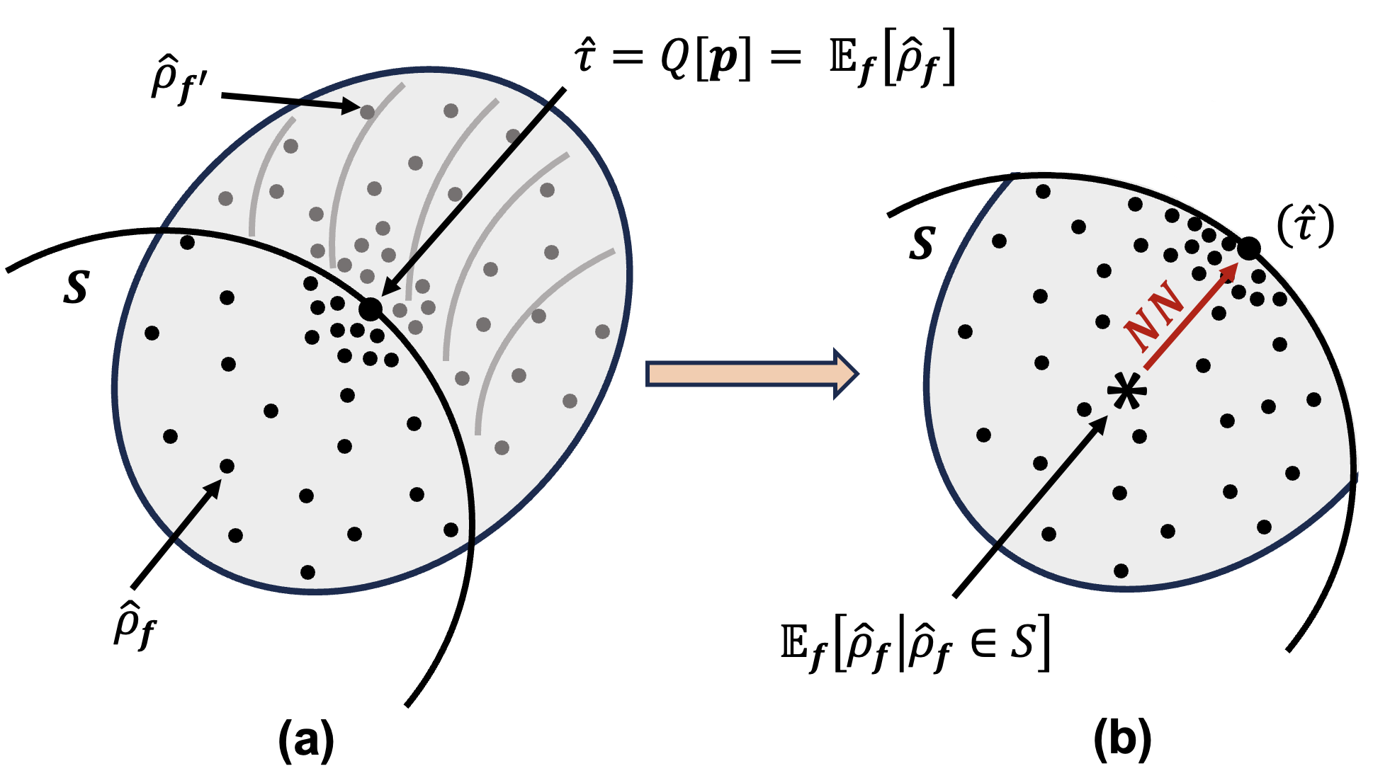
Figure 4: Action of the NN as a conditional debiaser. (a) Inference of the state $\hat{\tau}$ by many finite-size realization $\{\hat{\rho}_{\mathbf{f}}\}_{\mathbf{f}}$ not necesarily a proper state (i.e., it might be outside $\mathcal{S}$). (b) If we disregard the non-physical realizations, it results in a skewed conditional distribution whose mean is displaced from the true state. The action of the NN is then to shift back the mean to the target state by drifting the distribution.

As a result, generic mixed states are harder to improve than pure states. Further studies are necessary to confirm the said behavior. In particular, one has to verify that no improvement is possible if the reconstruction method to obtain $\hat{\rho}_{\mathbf{f}}$ already incorporates the skewness and how the performance depends on the bias of the estimator $Q$.

Appendix E Sampling random states

We want the algorithm to learn how noise affects generic states covering the whole space $\mathcal{S}$ of proper quantum states. In doing so, we will have a flexible solution with the potential to improve any state. To this end, we will train our NN with random states sampled from different measures covering uniformly the volume of interest. In particular, for mixed states, we will use the Hilbert-Schmidt ensemble, while for pure states the Haar measure, In the following we review how to generate such random states:

Hilbert-Schmidt states.– The HS measure is defined by the infinitesimal line element:

$$ds_{\mathrm{HS}}^{2}=\mathrm{Tr}[(d\hat{\tau}_{\mathrm{HS}})^{2}],$$ (31)

which indeed induces the HS-distance $D_{\mathrm{HS}}$, as defined in Eq. (8), once integrated.

States uniformly distributed in the space endowed with the corresponding metric, Eq. (31), may be sampled as:

$$\hat{\tau}_{\mathrm{HS}}=\frac{AA^{\dagger}}{\mathrm{Tr}[AA^{\dagger}]},$$ (32)

where $A$ is a generic complex square matrix whose real and imaginary matrix elements are i.i.d. sampled normal random variables $\mathcal{N}(0,1)$.

Haar vectors.– Such ensemble is defined on the pure state space $\hat{\tau}=\outerproduct{\Psi}{\Psi}$ and may be used to infer states with high purity, as the metrologically useful states explored in the main text. Formally, it takes advantage of the link between states $\ket{\Psi}\in\mathcal{H}$, and the unitary group. The fundamental property of such measure is that it is invariant under unitary transformations, thus making any vector in $\mathcal{H}$ equiprobable.

Interestingly, Haar vectors (or equivalently unitaries), can be drawn again from i.i.d. random normal variables $\mathcal{N}(0,1)$ Mezzadri (2007). Let $A$ be a complex square matrix sampled as before. Then, we apply the so called QR decomposition:

$$A=QR,$$ (33)

where $Q$ is unitary and $R$ is upper-triangular. Then $Q^{\prime}=Q\Lambda$, where $\Lambda=\mathrm{diag}(\{R_{\alpha\alpha}/|R_{\alpha\alpha}|\}_{\alpha})$, is Haar random.

In practice, we may use the python package qutip to compute those. For further information on random states, we refer to the book Ref. Bengtsson and Życzkowski (2017).

Appendix F Improving the averaged MLE in HS metric

The MLE is efficient asymptotically, with a number of measurements $N\to\infty$. However, for a few number of measurements, there is no guarantee that MLE performs best. Such a situation takes place in the undersampled regime. In terms of the HS metric, it is usually more convenient to disregard any knowledge and just take the maximally mixed state $\mathbb{1}/d$ as an estimation. Here, we propose a simple method to interpolate between the two extreme results by depolarizing the MLE state $\hat{\rho}$,

$$\hat{\rho}_{p}=p\hat{\rho}+(1-p)\mathbb{1}/d\ ,$$ (34)

with $0\leq p\leq 1$. The parameter $p$, then, would incorporate the statistical noise inherent to have a finite number of samples.

In Fig. 5 we show the average HS distance as a function of a number of trails $N_{\rm trial}$, for different values of the parameter $p$. The first extreme case ($p=0$) i.e. maximally mixed state is presented as a horizontal solid line, while the second extreme case ($p=1$), i.e. MLE reconstructed state is depicted as a dashed line. All intermediate values of $p$ form an envelope shape, which corresponds to a critical value $p^{*}$, outperforming all other values of $p$.

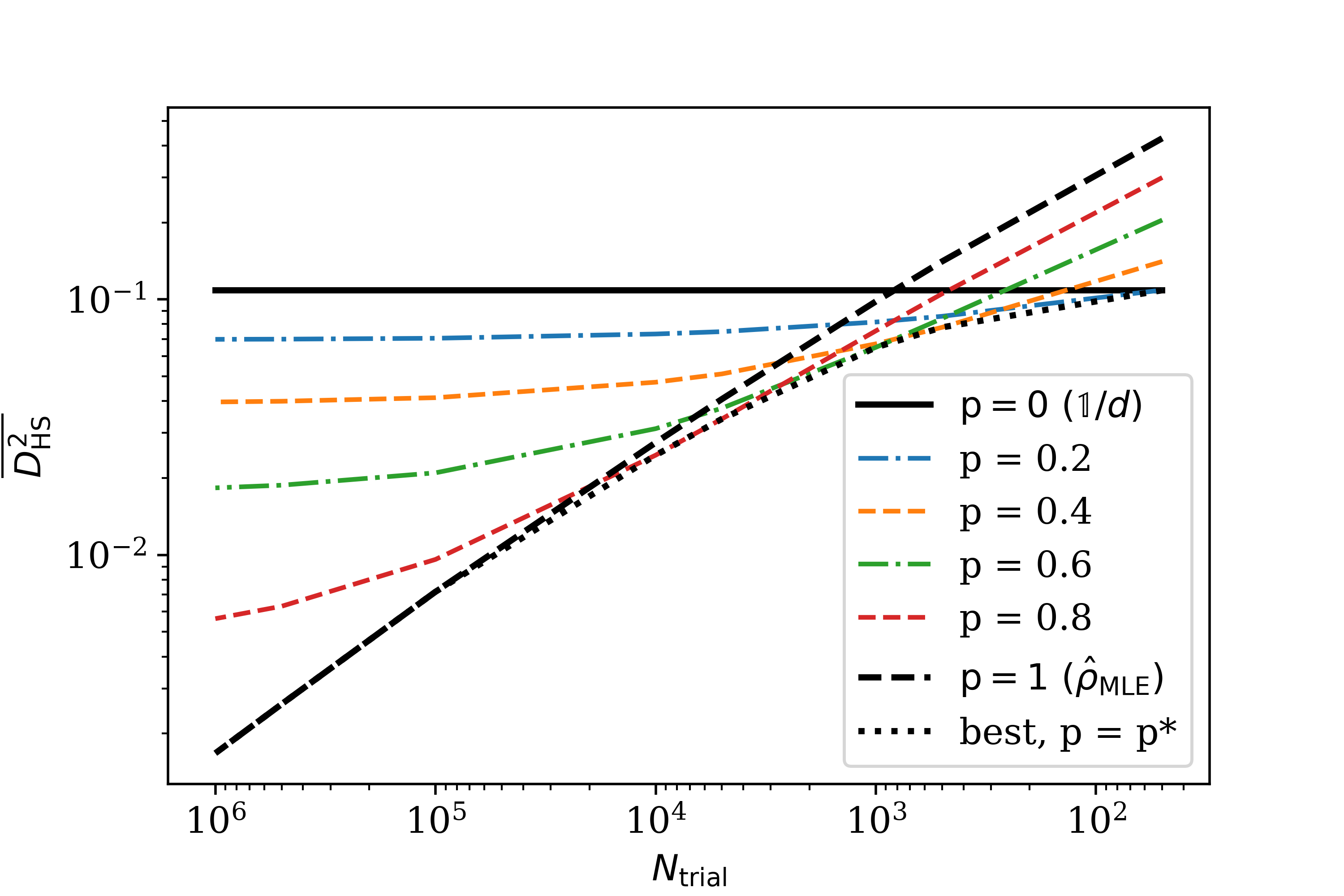
Figure 5: Averaged HS distance of reconstructed MLE from the HS ensemble with $d=9$ as mixed according to Eq.  (34) for different values of $p$ (colored lines). We highlight the limiting cases, namely $p=0$ (solid line); the average with respect $\mathbb{1}/d$, and $p=1$ (dashed): the MLE result. The envelope of such a family of lines is marked with a dotted line. Such bound can be realized with an optimal $p_{*}$, which depends on the number of trials via the reconstructed $\{\hat{\rho}_{\mathrm{MLE}}\}$.

To calculate the critical $p^{*}$ let us notice that the average of the squared HS distance with respect to the state Eq. (34), $D_{p}^{2}=D_{\mathrm{HS}}^{2}(\hat{\tau},\hat{\rho}_{p})$, can be expressed as,

$$D_{p}^{2}=D_{0}^{2}+(D_{1}^{2}-D_{0}^{2}-D_{01}^{2})p+D_{01}^{2}p^{2}\ ,$$ (35)

where,

$$D_{0}^{2} =D^{2}_{\mathrm{HS}}(\hat{\tau},\mathbb{1}/d)$$ (36)

$$D_{1}^{2} =D^{2}_{\mathrm{HS}}(\hat{\tau},\hat{\rho}_{\mathrm{MLE}})$$ (37)

$$D_{01}^{2} =D^{2}_{\mathrm{HS}}(\mathbb{1}/d,\hat{\rho}_{\mathrm{MLE}})$$ (38)

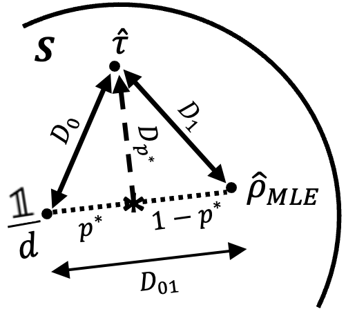
Figure 6: Geometric interpretation of the optimal depolarization of the MLE state, such as to incorporate the statistical noise stemming from a finite number of experimental runs.

The Eq. (35) is equally valid in average as it is linear in the $D^{2}$’s and we consider $p$ a global parameter. Then, $\overline{D_{0}^{2}}$ can be related to the average purity $\overline{\mathrm{Tr}(\hat{\tau}^{2})}$ as $D_{0}^{2}=\mathrm{Tr}(\hat{\tau}^{2})-d^{-1}$. Also, as depicted in Fig. 6, it can be interpreted geometrically as a triangle of sides’ length $\{D_{0},D_{1},D_{01}\}$ in which we want to find the point $p$ in the segment $01$ which is closer to the opposed vertex. Minimization of the same equation leads to the optimal $p^{*}$:

$$p_{*}=\begin{cases}0&\overline{D_{01}^{2}}<\overline{D_{1}^{2}-D_{0}^{2}}\\ \frac{\overline{D_{01}^{2}+D_{0}^{2}-D_{1}^{2}}}{2\overline{D_{01}^{2}}}&\mbox{otherwise}\\ 1&\overline{D_{01}^{2}}<\overline{D_{0}^{2}-D_{1}^{2}}\\ \end{cases}\ ,$$ (39)

yielding an optimal distance:

$$\overline{D_{*}^{2}}=\begin{cases}\overline{D_{0}^{2}}&\overline{D_{01}^{2}}<\overline{D_{1}^{2}-D_{0}^{2}}\\ \overline{D_{0}^{2}}-\frac{\overline{D_{0}^{2}-D_{1}^{2}-D_{01}^{2}}^{2}}{4\overline{D_{01}^{2}}}&\mbox{otherwise}\\ \overline{D_{1}^{2}}&\overline{D_{01}^{2}}<\overline{D_{0}^{2}-D_{1}^{2}}\\ \end{cases}\ ,$$ (40)

In Fig. 7, we observe a realization of the nontrivial solution (otherwise case), which is better than both $\overline{D_{0}^{2}}$ and $\overline{D_{1}^{2}}$.

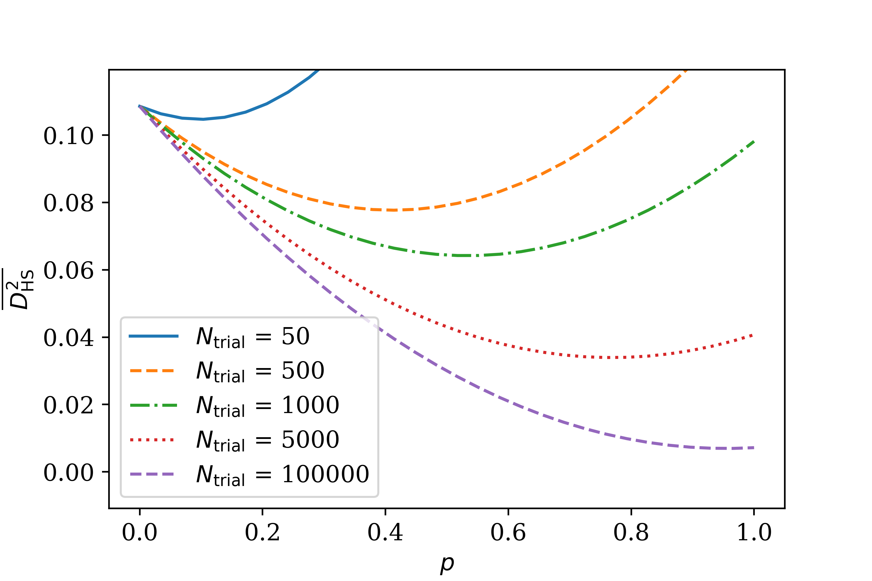
Figure 7: Average reconstruction distance as a function of the mixing parameter $p$ for a given set of number of trials. We verify the parabola curves of Eq. (35) and the nontrivial minima.

Finally, one should check how such a method relates to Bayesian approaches Granade et al. (2016). In particular, how to incorporate partial information about the ensemble, e.g., by only assuming as prior knowledge an average purity.

Appendix G Capturing the metrological usefulness of OAT evolved states

Given a quantum state $\hat{\rho}$ with spectral decomposition $\hat{\rho}=\sum_{k}p_{k}\outerproduct{k}{k}$, we can evaluate its sensitivity upon rotations generated by $\hat{G}$, $\hat{\rho}(\theta)=e^{-i\theta\hat{G}}\hat{\rho}e^{+i\theta\hat{G}}$ as quantified by the QFI:

$$F_{Q}[\hat{\rho},\hat{G}]=2\sum_{\begin{subarray}{c}k,l\\ p_{k}+p_{l}>0\end{subarray}}\frac{(p_{k}-p_{l})^{2}}{p_{k}+p_{l}}|\bra{k}\hat{G}\ket{l}|^{2}.$$ (41)

In the main text, we consider an ensemble of $L$ spins-$1/2$, or two-level atoms. In such system and in the context of magnetometry (e.g., via Ramsey interferometry), the phase is encoded the same way in every constituent via the collective generator $\hat{J}_{\mathbf{v}}=\sum_{i\in[L]}\mathbf{v}\cdot\hat{\bm{\sigma}}_{i}$ where $\mathbf{v}=(v_{x},v_{y},v_{z})$ is the encoding orientation.

For a generic state $\hat{\rho}$, it is not direct to find the optimal spatial direction $\mathbf{v}$ to exploit the maximal sensitivity. However, for pure states $\hat{\rho}=\outerproduct{\Psi}{\Psi}$ (like the OAT evolution that we consider), the QFI is (four times) the variance of the generator, $F_{Q}[\ket{\Psi},\hat{G}]=4[\bra{\Psi}\hat{G}^{2}\ket{\Psi}-\bra{\Psi}\hat{G}\ket{\Psi}^{2}]$ and the best direction is then yielded by the maximal eigenvalue $\mathbf{v}_{\rm max}$ of the covariance matrix $\mathcal{C}$:

$$\mathcal{C}= \begin{pmatrix}\langle\hat{J}_{x}^{2}\rangle&\mathrm{Re}\{\langle\hat{J}_{x}\hat{J}_{y}\rangle\}&\mathrm{Re}\{\langle\hat{J}_{x}\hat{J}_{z}\rangle\}\\ \mathrm{Re}\{\langle\hat{J}_{x}\hat{J}_{y}\rangle\}&\langle\hat{J}_{y}^{2}\rangle&\mathrm{Re}\{\langle\hat{J}_{y}J_{z}\rangle\}\\ \mathrm{Re}\{\langle\hat{J}_{x}\hat{J}_{z}\rangle\}&\mathrm{Re}\{\langle\hat{J}_{y}\hat{J}_{z}\rangle\}&\langle\hat{J}_{z}^{2}\rangle\end{pmatrix}$$ (42)

$$-\begin{pmatrix}\langle\hat{J}_{x}\rangle\\ \langle\hat{J}_{y}\rangle\\ \langle\hat{J}_{z}\rangle\end{pmatrix}\begin{pmatrix}\langle\hat{J}_{x}\rangle&\langle\hat{J}_{y}\rangle&\langle\hat{J}_{z}\rangle\end{pmatrix},$$

where the expectation value is taken against pure states, $\langle\cdot\rangle:=\bra{\Psi}\cdot\ket{\Psi}$. The maximal value of the QFI achieved is consequently $F_{Q}[\ket{\Psi},J_{\mathbf{v}_{\mathrm{best}}=\mathbf{v}_{\max}}]=4\mathbf{v}_{\max}^{T}\mathcal{C}\mathbf{v}_{\max}=4\lambda_{\max}(\mathcal{C})$, where $\lambda_{\max}$ indicates maximal eigenvalue. Here, we will introduce two basic examples of such result:

• A coherent spin state pointing along $x$ of length $J=L/2$, $\ket{+}^{\otimes L}$. This is the initial state chosen to start OAT dynamics, Eq. (9) (main text). In such case, the optimal axis is any orientation orthogonal to $x$, i.e. contained in the $yz$ plane. The QFI achieved is exactly $L$, which is the maximal value that can be reached by separable states (a.k.a. shot noise limit) Pezzé and Smerzi (2009).

• The GHZ or cat state aligned along $x$, $(|+\rangle^{\otimes L}+e^{i\phi}|-\rangle^{\otimes L})/\sqrt{2}$, which is realized at time $t=\pi/2$ during the OAT dynamics. Now, the optimal generator points in the $x$ direction and the corresponding QFI (variance times four) is $L^{2}$. Such value actually is the maximal QFI achievable within the quantum framework and requires genuine $L$-partite entanglement Hyllus et al. (2012); Tóth (2012).

Since the OAT reconstructed states $\hat{\rho}$ are of high purity, the same procedure can be used to approximate the optimal orientation $\mathbf{v}$. However, the QFI results are evaluated exactly as per Eq. (41). For further study, we refer the reader to the excellent review of Ref. Pezzè et al. (2018).

References

- Gühne and Tóth (2009) O. Gühne and G. Tóth, Physics Reports 474, 1 (2009).
- da Silva et al. (2011) M. P. da Silva, O. Landon-Cardinal, and D. Poulin, Phys. Rev. Lett. 107, 210404 (2011).
- Kliesch and Roth (2021) M. Kliesch and I. Roth, PRX Quantum 2, 010201 (2021).
- Tavakoli (2020) A. Tavakoli, Phys. Rev. Lett. 125, 150503 (2020).
- Friis et al. (2019) N. Friis, G. Vitagliano, M. Malik, and M. Huber, Nature Reviews Physics 1, 72 (2019).
- Eisert et al. (2020) J. Eisert, D. Hangleiter, N. Walk, I. Roth, D. Markham, R. Parekh, U. Chabaud, and E. Kashefi, Nature Reviews Physics 2, 382 (2020).
- Sotnikov et al. (2022) O. M. Sotnikov, I. A. Iakovlev, A. A. Iliasov, M. I. Katsnelson, A. A. Bagrov, and V. V. Mazurenko, npj Quantum Information 8, 41 (2022).
- Chen et al. (2022) S. Chen, J. Li, B. Huang, and A. Liu, in 2022 IEEE 63rd Annual Symposium on Foundations of Computer Science (FOCS) (IEEE Computer Society, Los Alamitos, CA, USA, 2022) pp. 1205–1213.
- Gočanin et al. (2022) A. Gočanin, I. Šupić, and B. Dakić, PRX Quantum 3, 010317 (2022).
- Boghiu et al. (2023) E.-C. Boghiu, F. Hirsch, P.-S. Lin, M. T. Quintino, and J. Bowles, SciPost Phys. Core 6, 028 (2023).
- Leonhardt (1995) U. Leonhardt, Phys. Rev. Lett. 74, 4101 (1995).
- White et al. (1999) A. G. White, D. F. V. James, P. H. Eberhard, and P. G. Kwiat, Phys. Rev. Lett. 83, 3103 (1999).
- Roos et al. (2004) C. F. Roos, G. P. T. Lancaster, M. Riebe, H. Häffner, W. Hänsel, S. Gulde, C. Becher, J. Eschner, F. Schmidt-Kaler, and R. Blatt, Phys. Rev. Lett. 92, 220402 (2004).
- Häffner et al. (2005) H. Häffner, W. Hänsel, C. F. Roos, J. Benhelm, D. Chek-al kar, M. Chwalla, T. Körber, U. D. Rapol, M. Riebe, P. O. Schmidt, C. Becher, O. Gühne, W. Dür, and R. Blatt, Nature 438, 643 (2005).
- Gross et al. (2010a) D. Gross, Y.-K. Liu, S. T. Flammia, S. Becker, and J. Eisert, Phys. Rev. Lett. 105, 150401 (2010a).
- Gross (2011) D. Gross, IEEE Transactions on Information Theory 57, 1548 (2011).
- Tóth et al. (2010a) G. Tóth, W. Wieczorek, D. Gross, R. Krischek, C. Schwemmer, and H. Weinfurter, Phys. Rev. Lett. 105, 250403 (2010a).
- Moroder et al. (2012) T. Moroder, P. Hyllus, G. Tóth, C. Schwemmer, A. Niggebaum, S. Gaile, O. Gühne, and H. Weinfurter, New Journal of Physics 14, 105001 (2012).
- Cramer et al. (2010) M. Cramer, M. B. Plenio, S. T. Flammia, R. Somma, D. Gross, S. D. Bartlett, O. Landon-Cardinal, D. Poulin, and Y.-K. Liu, Nature Communications 1 (2010), 10.1038/ncomms1147.
- Baumgratz et al. (2013) T. Baumgratz, D. Gross, M. Cramer, and M. B. Plenio, Phys. Rev. Lett. 111, 020401 (2013).
- Lanyon et al. (2017) B. P. Lanyon, C. Maier, M. Holzäpfel, T. Baumgratz, C. Hempel, P. Jurcevic, I. Dhand, A. S. Buyskikh, A. J. Daley, M. Cramer, M. B. Plenio, R. Blatt, and C. F. Roos, Nature Physics 13, 1158 (2017).
- Acín et al. (2018) A. Acín, I. Bloch, H. Buhrman, T. Calarco, C. Eichler, J. Eisert, D. Esteve, N. Gisin, S. J. Glaser, F. Jelezko, S. Kuhr, M. Lewenstein, M. F. Riedel, P. O. Schmidt, R. Thew, A. Wallraff, I. Walmsley, and F. K. Wilhelm, New Journal of Physics 20, 080201 (2018).
- Kinos et al. (2021) A. Kinos, D. Hunger, R. Kolesov, K. Mølmer, H. de Riedmatten, P. Goldner, A. Tallaire, L. Morvan, P. Berger, S. Welinski, K. Karrai, L. Rippe, S. Kröll, and A. Walther, “Roadmap for rare-earth quantum computing,” (2021).
- Laucht et al. (2021) A. Laucht, F. Hohls, N. Ubbelohde, M. F. Gonzalez-Zalba, D. J. Reilly, S. Stobbe, T. Schröder, P. Scarlino, J. V. Koski, A. Dzurak, C.-H. Yang, J. Yoneda, F. Kuemmeth, H. Bluhm, J. Pla, C. Hill, J. Salfi, A. Oiwa, J. T. Muhonen, E. Verhagen, M. D. LaHaye, H. H. Kim, A. W. Tsen, D. Culcer, A. Geresdi, J. A. Mol, V. Mohan, P. K. Jain, and J. Baugh, Nanotechnology 32, 162003 (2021).
- Becher et al. (2022) C. Becher, W. Gao, S. Kar, C. Marciniak, T. Monz, J. G. Bartholomew, P. Goldner, H. Loh, E. Marcellina, K. E. J. Goh, T. S. Koh, B. Weber, Z. Mu, J.-Y. Tsai, Q. Yan, S. Gyger, S. Steinhauer, and V. Zwiller, “2022 roadmap for materials for quantum technologies,” (2022).
- Fraxanet et al. (2022) J. Fraxanet, T. Salamon, and M. Lewenstein, “The coming decades of quantum simulation,” (2022).
- Gross et al. (2010b) D. Gross, Y.-K. Liu, S. T. Flammia, S. Becker, and J. Eisert, Phys. Rev. Lett. 105, 150401 (2010b).
- Flammia et al. (2012) S. T. Flammia, D. Gross, Y.-K. Liu, and J. Eisert, New Journal of Physics 14, 095022 (2012).
- Huszár and Houlsby (2012) F. Huszár and N. M. T. Houlsby, Phys. Rev. A 85, 052120 (2012).
- Kravtsov et al. (2013) K. S. Kravtsov, S. S. Straupe, I. V. Radchenko, N. M. T. Houlsby, F. Huszár, and S. P. Kulik, Phys. Rev. A 87, 062122 (2013).
- Granade et al. (2017) C. Granade, C. Ferrie, and S. T. Flammia, New Journal of Physics 19, 113017 (2017).
- Tóth et al. (2010b) G. Tóth, W. Wieczorek, D. Gross, R. Krischek, C. Schwemmer, and H. Weinfurter, Phys. Rev. Lett. 105, 250403 (2010b).
- Schwemmer et al. (2014) C. Schwemmer, G. Tóth, A. Niggebaum, T. Moroder, D. Gross, O. Gühne, and H. Weinfurter, Phys. Rev. Lett. 113, 040503 (2014).
- Huang et al. (2020) H.-Y. Huang, R. Kueng, and J. Preskill, Nature Physics 16, 1050 (2020).
- Aaronson (2020) S. Aaronson, SIAM Journal on Computing 49, STOC18 (2020).
- Cattaneo et al. (2023) M. Cattaneo, M. A. C. Rossi, K. Korhonen, E.-M. Borrelli, G. García-Pérez, Z. Zimborás, and D. Cavalcanti, Phys. Rev. Res. 5, 033154 (2023).
- Dawid et al. (2022) A. Dawid, J. Arnold, B. Requena, A. Gresch, M. Płodzień, K. Donatella, K. A. Nicoli, P. Stornati, R. Koch, M. Büttner, R. Okuła, G. Muñoz-Gil, R. A. Vargas-Hernández, A. Cervera-Lierta, J. Carrasquilla, V. Dunjko, M. Gabrié, P. Huembeli, E. van Nieuwenburg, F. Vicentini, L. Wang, S. J. Wetzel, G. Carleo, E. Greplová, R. Krems, F. Marquardt, M. Tomza, M. Lewenstein, and A. Dauphin, “Modern applications of machine learning in quantum sciences,” (2022), arXiv:2204.04198 [quant-ph] .
- Torlai et al. (2018) G. Torlai, G. Mazzola, J. Carrasquilla, M. Troyer, R. Melko, and G. Carleo, Nature Physics 14, 447 (2018).
- Carrasquilla et al. (2019) J. Carrasquilla, G. Torlai, R. G. Melko, and L. Aolita, Nature Machine Intelligence 1, 155 (2019).
- Cha et al. (2021) P. Cha, P. Ginsparg, F. Wu, J. Carrasquilla, P. L. McMahon, and E.-A. Kim, Machine Learning: Science and Technology 3, 01LT01 (2021).
- Melkani et al. (2020) A. Melkani, C. Gneiting, and F. Nori, Phys. Rev. A 102, 022412 (2020).
- Schmale et al. (2022) T. Schmale, M. Reh, and M. Gärttner, npj Quantum Information 8 (2022), 10.1038/s41534-022-00621-4.
- Xin et al. (2019) T. Xin, S. Lu, N. Cao, G. Anikeeva, D. Lu, J. Li, G. Long, and B. Zeng, npj Quantum Information 5 (2019), 10.1038/s41534-019-0222-3.
- Palmieri et al. (2020) A. Palmieri, E. Kovlakov, F. Bianchi, D. Yudin, S. Straupe, J. D. Biamonte, and S. Kulik, npj Quantum Inf 6, 20 (2020).
- Pan and Zhang (2022) C. Pan and J. Zhang, International Journal of Theoretical Physics 61 (2022), 10.1007/s10773-022-05209-4.
- Koutný et al. (2022) D. Koutný, L. Motka, Z. c. v. Hradil, J. Řeháček, and L. L. Sánchez-Soto, Phys. Rev. A 106, 012409 (2022).
- Ahmed et al. (2021) S. Ahmed, C. Sánchez Muñoz, F. Nori, and A. F. Kockum, Phys. Rev. Lett. 127, 140502 (2021).
- Zhao et al. (2023) H. Zhao, G. Carleo, and F. Vicentini, “Empirical sample complexity of neural network mixed state reconstruction,” (2023), arXiv:2307.01840 [quant-ph] .
- Carrasquilla and Torlai (2021) J. Carrasquilla and G. Torlai, PRX Quantum 2, 040201 (2021).
- Westerhout et al. (2020) T. Westerhout, N. Astrakhantsev, K. S. Tikhonov, M. I. Katsnelson, and A. A. Bagrov, Nature Communications 11 (2020), 10.1038/s41467-020-15402-w.
- Fuchs and Schack (2013) C. A. Fuchs and R. Schack, Reviews of Modern Physics 85, 1693 (2013).
- Fuchs et al. (2017) C. Fuchs, M. Hoang, and B. Stacey, Axioms 6, 21 (2017).
- Peter and Petrosyan (2007) L. Peter and D. Petrosyan, Fundamentals of quantum optics and quantum information (Springer, Berlin, 2007).
- Goodfellow et al. (2016) I. Goodfellow, Y. Bengio, and A. Courville, Deep Learning (MIT Press, 2016) http://www.deeplearningbook.org.
- Zhu et al. (2022) Y. Zhu, Y.-D. Wu, G. Bai, D.-S. Wang, Y. Wang, and G. Chiribella, Nature Communications 13 (2022), 10.1038/s41467-022-33928-z.
- Requena et al. (2023) B. Requena, S. Masó, J. Bertran, M. Lewenstein, C. Manzo, and G. Muñoz-Gil, “Inferring pointwise diffusion properties of single trajectories with deep learning,” (2023).
- Bahdanau et al. (2016) D. Bahdanau, K. Cho, and Y. Bengio, “Neural machine translation by jointly learning to align and translate,” (2016), arXiv:1409.0473 [cs.CL] .
- Vaswani et al. (2023) A. Vaswani, N. Shazeer, N. Parmar, J. Uszkoreit, L. Jones, A. N. Gomez, L. Kaiser, and I. Polosukhin, “Attention is all you need,” (2023), arXiv:1706.03762 [cs.CL] .
- Dwivedi and Bresson (2021) V. P. Dwivedi and X. Bresson, “A generalization of transformer networks to graphs,” (2021), arXiv:2012.09699 [cs.LG] .
- Hendrycks and Gimpel (2023) D. Hendrycks and K. Gimpel, “Gaussian error linear units (gelus),” (2023), arXiv:1606.08415 [cs.LG] .
- Liu et al. (2023) T. Liu, S. Liu, H. Li, H. Li, K. Huang, Z. Xiang, X. Song, K. Xu, D. Zheng, and H. Fan, Nature Communications 14 (2023), 10.1038/s41467-023-37511-y.
- Tang et al. (2022) H. Tang, L. Banchi, T.-Y. Wang, X.-W. Shang, X. Tan, W.-H. Zhou, Z. Feng, A. Pal, H. Li, C.-Q. Hu, M. Kim, and X.-M. Jin, Physical Review Letters 128 (2022), 10.1103/physrevlett.128.050503.
- Kitagawa and Ueda (1993a) M. Kitagawa and M. Ueda, Phys. Rev. A 47, 5138 (1993a).
- Wineland et al. (1994a) D. Wineland, J. Bollinger, W. Itano, and D. Heinzen, Phys. Rev. A 50, 67 (1994a).
- Pezzè et al. (2018) L. Pezzè, A. Smerzi, M. K. Oberthaler, R. Schmied, and P. Treutlein, Rev. Mod. Phys. 90, 035005 (2018).
- Wolfgramm et al. (2010) F. Wolfgramm, A. Cerè, F. A. Beduini, A. Predojević, M. Koschorreck, and M. W. Mitchell, Phys. Rev. Lett. 105, 053601 (2010).
- Wineland et al. (1994b) D. J. Wineland, J. J. Bollinger, W. M. Itano, and D. J. Heinzen, Phys. Rev. A 50, 67 (1994b).
- Müller-Rigat et al. (2023) G. Müller-Rigat, A. K. Srivastava, S. Kurdziałek, G. Rajchel-Mieldzioć, M. Lewenstein, and I. Frérot, “Certifying the quantum fisher information from a given set of mean values: a semidefinite programming approach,” (2023).
- Tura et al. (2014) J. Tura, R. Augusiak, A. B. Sainz, T. Vértesi, M. Lewenstein, and A. Acín, Science 344, 1256 (2014).
- Schmied et al. (2016) R. Schmied, J.-D. Bancal, B. Allard, M. Fadel, V. Scarani, P. Treutlein, and N. Sangouard, Science 352, 441 (2016).
- Aloy et al. (2019) A. Aloy, J. Tura, F. Baccari, A. Acín, M. Lewenstein, and R. Augusiak, Phys. Rev. Lett. 123, 100507 (2019).
- Baccari et al. (2019) F. Baccari, J. Tura, M. Fadel, A. Aloy, J.-D. Bancal, N. Sangouard, M. Lewenstein, A. Acín, and R. Augusiak, Phys. Rev. A 100, 022121 (2019).
- Tura et al. (2019) J. Tura, A. Aloy, F. Baccari, A. Acín, M. Lewenstein, and R. Augusiak, Phys. Rev. A 100, 032307 (2019).
- Müller-Rigat et al. (2021) G. Müller-Rigat, A. Aloy, M. Lewenstein, and I. Frérot, PRX Quantum 2, 030329 (2021).
- Żukowski and Brukner (2002) M. Żukowski and Č. Brukner, Phys. Rev. Lett. 88, 210401 (2002).
- Cavalcanti et al. (2007) E. G. Cavalcanti, C. J. Foster, M. D. Reid, and P. D. Drummond, Phys. Rev. Lett. 99, 210405 (2007).
- He et al. (2011) Q. He, P. Drummond, and M. Reid, Phys. Rev. A 83, 032120 (2011).
- Cavalcanti et al. (2011) E. Cavalcanti, Q. He, M. Reid, and H. Wiseman, Phys. Rev. A 84, 032115 (2011).
- Niezgoda et al. (2020) A. Niezgoda, M. Panfil, and J. Chwedeńczuk, Phys. Rev. A 102, 042206 (2020).
- Niezgoda and Chwedeńczuk (2021) A. Niezgoda and J. Chwedeńczuk, Phys. Rev. Lett. 126, 210506 (2021).
- Chwedeńczuk (2022) J. Chwedeńczuk, SciPost Phys. Core 5, 25 (2022).
- Müller-Rigat et al. (2021) G. Müller-Rigat, A. Aloy, M. Lewenstein, and I. Frérot, PRX Quantum 2 (2021), 10.1103/prxquantum.2.030329.
- Wineland et al. (1992) D. J. Wineland, J. J. Bollinger, W. M. Itano, F. L. Moore, and D. J. Heinzen, Phys. Rev. A 46, R6797 (1992).
- Kitagawa and Ueda (1993b) M. Kitagawa and M. Ueda, Phys. Rev. A 47, 5138 (1993b).
- Gietka et al. (2015) K. Gietka, P. Szańkowski, T. Wasak, and J. Chwedeńczuk, Phys. Rev. A 92, 043622 (2015).
- Li et al. (2008) Y. Li, Y. Castin, and A. Sinatra, Phys. Rev. Lett. 100, 210401 (2008).
- Li et al. (2009) Y. Li, P. Treutlein, J. Reichel, and A. Sinatra, The European Physical Journal B 68, 365 (2009).
- Wang et al. (2017) M. Wang, W. Qu, P. Li, H. Bao, V. Vuletić, and Y. Xiao, Phys. Rev. A 96, 013823 (2017).
- Kajtoch et al. (2018a) D. Kajtoch, E. Witkowska, and A. Sinatra, EPL (Europhysics Letters) 123, 20012 (2018a).
- Schulte et al. (2020) M. Schulte, C. Lisdat, P. O. Schmidt, U. Sterr, and K. Hammerer, Nature Communications 11, 5955 (2020).
- Gietka et al. (2021) K. Gietka, A. Usui, J. Deng, and T. Busch, Phys. Rev. Lett. 126, 160402 (2021).
- Comparin et al. (2022) T. Comparin, F. Mezzacapo, and T. Roscilde, Phys. Rev. A 105, 022625 (2022).
- Riedel et al. (2010) M. F. Riedel, P. Böhi, Y. Li, T. W. Hänsch, A. Sinatra, and P. Treutlein, Nature 464, 1170–1173 (2010).
- Gross et al. (2010c) C. Gross, T. Zibold, E. Nicklas, J. Estève, and M. K. Oberthaler, Nature 464, 1165–1169 (2010c).
- Hamley et al. (2012) C. D. Hamley, C. S. Gerving, T. M. Hoang, E. M. Bookjans, and M. S. Chapman, Nature Physics 8, 305–308 (2012).
- Qu et al. (2020) A. Qu, B. Evrard, J. Dalibard, and F. Gerbier, Phys. Rev. Lett. 125, 033401 (2020).
- Leroux et al. (2010) I. D. Leroux, M. H. Schleier-Smith, and V. Vuletić, Phys. Rev. Lett. 104, 073602 (2010).
- Maussang et al. (2010) K. Maussang, G. E. Marti, T. Schneider, P. Treutlein, Y. Li, A. Sinatra, R. Long, J. Estève, and J. Reichel, Phys. Rev. Lett. 105, 080403 (2010).
- Kajtoch et al. (2018b) D. Kajtoch, E. Witkowska, and A. Sinatra, EPL (Europhysics Letters) 123, 20012 (2018b).
- He et al. (2019) P. He, M. A. Perlin, S. R. Muleady, R. J. Lewis-Swan, R. B. Hutson, J. Ye, and A. M. Rey, Phys. Rev. Research 1, 033075 (2019).
- Płodzień et al. (2020) M. Płodzień, M. Kościelski, E. Witkowska, and A. Sinatra, Phys. Rev. A 102, 013328 (2020).
- Płodzień et al. (2022) M. Płodzień, M. Lewenstein, E. Witkowska, and J. Chwedeńczuk, Phys. Rev. Lett. 129, 250402 (2022).
- Płodzień et al. (2023) M. Płodzień, T. Wasak, E. Witkowska, M. Lewenstein, and J. Chwedeńczuk, “Generation of scalable many-body bell correlations in spin chains with short-range two-body interactions,” (2023), arXiv:2306.06173 [quant-ph] .
- Mamaev et al. (2021) M. Mamaev, I. Kimchi, R. M. Nandkishore, and A. M. Rey, Phys. Rev. Research 3, 013178 (2021).
- Hernández Yanes et al. (2022) T. Hernández Yanes, M. Płodzień, M. Mackoit Sinkevičienė, G. Žlabys, G. Juzeliūnas, and E. Witkowska, Phys. Rev. Lett. 129, 090403 (2022).
- Dziurawiec et al. (2023) M. Dziurawiec, T. H. Yanes, M. Płodzień, M. Gajda, M. Lewenstein, and E. Witkowska, Physical Review A 107 (2023), 10.1103/physreva.107.013311.
- Hernández Yanes et al. (2023) T. Hernández Yanes, G. Žlabys, M. Płodzień, D. Burba, M. M. Sinkevičienė, E. Witkowska, and G. Juzeliūnas, Phys. Rev. B 108, 104301 (2023).
- Hyllus et al. (2012) P. Hyllus, W. Laskowski, R. Krischek, C. Schwemmer, W. Wieczorek, H. Weinfurter, L. Pezzé, and A. Smerzi, Phys. Rev. A 85, 022321 (2012).
- Tóth (2012) G. Tóth, Phys. Rev. A 85, 022322 (2012).
- Pezzé and Smerzi (2009) L. Pezzé and A. Smerzi, Phys. Rev. Lett. 102, 100401 (2009).
- Macarone-Palmieri (2023) A. Macarone-Palmieri, “Data generation, test-sets and model training codes for attention-based-qst available here.” (2023).
- Tóth et al. (2010) G. Tóth, W. Wieczorek, D. Gross, R. Krischek, C. Schwemmer, and H. Weinfurter, Physical Review Letters 105 (2010), 10.1103/physrevlett.105.250403.
- Oszmaniec et al. (2016) M. Oszmaniec, R. Augusiak, C. Gogolin, J. Kołodyński, A. Acín, and M. Lewenstein, Phys. Rev. X 6, 041044 (2016).
- Smolin et al. (2012) J. A. Smolin, J. M. Gambetta, and G. Smith, Phys. Rev. Lett. 108, 070502 (2012).
- ApS (2019) M. ApS, The MOSEK optimization toolbox for MATLAB manual. Version 9.0. (2019).
- Aaronson and Rothblum (2019) S. Aaronson and G. N. Rothblum, in Proceedings of the 51st Annual ACM SIGACT Symposium on Theory of Computing, STOC 2019 (Association for Computing Machinery, New York, NY, USA, 2019) p. 322–333.
- Struchalin et al. (2021) G. Struchalin, Y. A. Zagorovskii, E. Kovlakov, S. Straupe, and S. Kulik, PRX Quantum 2, 010307 (2021).
- Zhang et al. (2021) T. Zhang, J. Sun, X.-X. Fang, X.-M. Zhang, X. Yuan, and H. Lu, Phys. Rev. Lett. 127, 200501 (2021).
- Seif et al. (2023) A. Seif, Z.-P. Cian, S. Zhou, S. Chen, and L. Jiang, PRX Quantum 4, 010303 (2023).
- Bengtsson and Życzkowski (2017) I. Bengtsson and K. Życzkowski, Geometry of Quantum States: An Introduction to Quantum Entanglement, 2nd ed. (Cambridge University Press, 2017).
- Silva et al. (2017) G. B. Silva, S. Glancy, and H. M. Vasconcelos, Physical Review A 95 (2017), 10.1103/physreva.95.022107.
- Ferrie and Blume-Kohout (2018) C. Ferrie and R. Blume-Kohout, “Maximum likelihood quantum state tomography is inadmissible,” (2018).
- Scholten and Blume-Kohout (2018) T. L. Scholten and R. Blume-Kohout, New Journal of Physics 20, 023050 (2018).
- Mezzadri (2007) F. Mezzadri, “How to generate random matrices from the classical compact groups,” (2007), arXiv:math-ph/0609050 [math-ph] .
- Granade et al. (2016) C. Granade, J. Combes, and D. G. Cory, New Journal of Physics 18, 033024 (2016).
- Pezzè et al. (2018) L. Pezzè, A. Smerzi, M. K. Oberthaler, R. Schmied, and P. Treutlein, Reviews of Modern Physics 90 (2018), 10.1103/revmodphys.90.035005.