An Extendable Python Implementation of Robust Optimisation Monte Carlo

Vasilis Gkolemis, Michael Gutmann, Henri Pesonen An Extendable Python Implementation of ROMC An Extendable ROMC implementation Performing inference in statistical models with an intractable likelihood is challenging, therefore, most likelihood-free inference (LFI) methods encounter accuracy and efficiency limitations. In this paper, we present the implementation of the LFI method Robust Optimisation Monte Carlo (ROMC) in the Python package ELFI. ROMC is a novel and efficient (highly-parallelizable) LFI framework that provides accurate weighted samples from the posterior. Our implementation can be used in two ways. First, a scientist may use it as an out-of-the-box LFI algorithm; we provide an easy-to-use API harmonized with the principles of ELFI, enabling effortless comparisons with the rest of the methods included in the package. Additionally, we have carefully split ROMC into isolated components for supporting extensibility. A researcher may experiment with novel method(s) for solving part(s) of ROMC without reimplementing everything from scratch. In both scenarios, the ROMC parts can run in a fully-parallelized manner, exploiting all CPU cores. We also provide helpful functionalities for (i) inspecting the inference process and (ii) evaluating the obtained samples. Finally, we test the robustness of our implementation on some typical LFI examples. Bayesian inference, implicit models, likelihood-free, Python, ELFI Bayesian inference, implicit models, likelihood-free, Python, ELFI Vasilis Gkolemis
Information Management Systems Institute (IMSI)
ATHENA Research and Innovation Center
Athens, Greece
E-mail:
URL: https://givasile.github.io

1 Introduction

Simulator-based models are particularly captivating due to the modeling freedom they provide. In essence, any data generating mechanism that can be written as a finite set of algorithmic steps can be programmed as a simulator-based model. Hence, these models are often used to model physical phenomena in the natural sciences such as, e.g., genetics, epidemiology or neuroscience gutmann2016; lintusaari2017; sisson2018; cranmer2020. In simulator-based models, it is feasible to generate samples using the simulator but is infeasible to evaluate the likelihood function. The intractability of the likelihood makes the so-called likelihood-free inference (LFI), i.e., the approximation of the posterior distribution without using the likelihood function, particularly challenging.

Optimization Monte Carlo (OMC), proposed by Meeds2015, is a novel LFI approach. The central idea is to convert the stochastic data-generating mechanism into a set of deterministic optimization processes. Afterwards, Forneron2016 described a similar method under the name ‘reverse sampler’. In their work, Ikonomov2019 identified some critical limitations of OMC, so they proposed Robust OMC (ROMC) an improved version of OMC with appropriate modifications.

In this paper, we present the implementation of ROMC at the Python package ELFI (Engine for likelihood-free inference) 1708.00707. The implementation has been designed to facilitate extensibility. ROMC is an LFI framework; it defines a sequence of algorithmic steps for approximating the posterior without enforcing a specific algorithm for each step. Therefore, a researcher may use ROMC as the backbone method and apply novel algorithms to each separate step. For being a ready-to-use LFI method, Ikonomov2019 propose a particular (default) algorithm for each step, but this choice is by no means restrictive. We have designed our software for facilitating such experimentation.

To the best of our knowledge, this is the first implementation of the ROMC inference method to a generic LFI framework. We organize the illustration and the evaluation of our implementation in three steps. First, for securing that our implementation is accurate, we test it against an artificial example with a tractable likelihood. The artificial example also serves as a step-by-step guide for showcasing the various functionalities of our implementation. Second, we use the second-order moving average (MA2) example Marin2012 from the ELFI package, using as ground truth the samples obtained with Rejection ABC lintusaari2017 using a very high number of samples. Finally, we present the execution times of ROMC, measuring the speed-up achieved by the parallel version of the implementation.

The code of the implementation is available at the official ELFI repository. Apart from the examples presented in the paper, there are five Google Colab Bisong2019 notebooks available online, with end-to-end examples illustrating how to: (i) use ROMC on a synthetic $1D$ example, (ii) use ROMC on a synthetic $2D$ example, (iii) use ROMC on the Moving Average example, (iv) extend ROMC with a Neural Network as a surrogate model, (v) extend ROMC with a custom proposal region module.

2 Background

We first give a short introduction to simulator-based models, we then focus on OMC and its robust version, ROMC, and we, finally, introduce ELFI, the Python package used for the implementation.

2.1 Simulator-based models and likelihood-free inference

An implicit or simulator-based model is a parameterized stochastic data generating mechanism, where we can sample data points but we cannot evaluate the likelihood. Formally, a simulator-based model is a parameterized family of probability density functions $\{p(\mathbf{y}|\boldsymbol{\theta})\}_{\boldsymbol{\theta}}$ whose closed-form is either unknown or computationally intractable. In these cases, we can only access the simulator $m_{r}(\boldsymbol{\theta})$, i.e., the black-box mechanism (computer code) that generates samples $\mathbf{y}$ in a stochastic manner from a set of parameters $\boldsymbol{\theta}\in\mathbb{R}^{D}$. We denote the process of obtaining samples from the simulator with $m_{r}(\boldsymbol{\theta})\rightarrow\mathbf{y}$. As shown by Meeds2015, it is feasible to isolate the randomness of the simulator by introducing a set of nuisance random variables denoted by $\mathbf{u}\sim p(\mathbf{u})$. Therefore, for a specific tuple $(\boldsymbol{\theta},\mathbf{u})$ the simulator becomes a deterministic mapping $g$, such that $\mathbf{y}=g(\boldsymbol{\theta},\mathbf{u})$. In terms of computer code, the randomness of a random process is governed by the global seed. There are some differences on how each scientific package handles the randomness; for example, at Numpy harris2020array the pseudo-random number generation is based on a global state, whereas, at JAX jax2018github random functions consume a key that is passed as a parameter. However, in all cases, setting the initial seed to a specific integer converts the simulation to a deterministic piece of code.

The modeling freedom of simulator-based models comes at the price of difficulties in inferring the parameters of interest. Denoting the observed data as $\mathbf{y_{0}}$, the main difficulty lies at the intractability of the likelihood function $L(\boldsymbol{\theta})=p(\mathbf{y_{0}}|\boldsymbol{\theta})$. To better see the sources of the intractability, and to address them, we go back to the basic characterization of the likelihood as the (rescaled) probability of generating data $\mathbf{y}$ that is similar to the observed data $\mathbf{y_{0}}$, using parameters $\boldsymbol{\theta}$. Formally, the likelihood $L(\boldsymbol{\theta})$ is:

$$L(\boldsymbol{\theta})=\lim_{\epsilon\to 0}c_{\epsilon}\int_{\mathbf{y}\in B_{d,\epsilon}(\mathbf{y_{0}})}p(\mathbf{y}|\boldsymbol{\theta})d\mathbf{y}=\lim_{\epsilon\to 0}c_{\epsilon}\Pr(g(\boldsymbol{\theta},\mathbf{u})\in B_{d,\epsilon}(\mathbf{y_{0}})\mid\boldsymbol{\theta})$$ (1)

where $c_{\epsilon}$ is a proportionality factor that depends on $\epsilon$ and $B_{d,\epsilon}(\mathbf{y_{0}})$ is an $\epsilon$ region around $\mathbf{y_{0}}$ that is defined through a distance function $d$, i.e.,  $B_{d,\epsilon}(\mathbf{y_{0}}):=\{\mathbf{y}:d(\mathbf{y},\mathbf{y_{0}})\leq\epsilon\}$. In cases where the output $\mathbf{y}$ belongs to a high dimensional space, it is common to extract summary statistics $\Phi$ before applying the distance $d$. In these cases, the $\epsilon$-region is defined as $B_{d,\epsilon}(\mathbf{y_{0}}):=\{\mathbf{y}:d(\Phi(\mathbf{y}),\Phi(\mathbf{y_{0}}))\leq\epsilon\}$. In our notation, the summary statistics are sometimes omitted for simplicity. Equation 1 highlights the main source of intractability; computing $\Pr(g(\boldsymbol{\theta},\mathbf{u})\in B_{d,\epsilon}(\mathbf{y_{0}})|\boldsymbol{\theta})$ as the fraction of samples that lie inside the $\epsilon$ region around $\mathbf{y_{0}}$ is computationally infeasible in the limit where $\epsilon\to 0$. Hence, the constraint is relaxed to $\epsilon>0$, which leads to the approximate likelihood:

$$L_{d,\epsilon}(\boldsymbol{\theta})=\Pr(\mathbf{y}\in B_{d,\epsilon}(\mathbf{y_{0}})\mid\boldsymbol{\theta}),\quad\text{where }\epsilon>0.$$ (2)

and, in turn, to the approximate posterior:

$$p_{d,\epsilon}(\boldsymbol{\theta}|\mathbf{y_{0}})\propto L_{d,\epsilon}(\boldsymbol{\theta})p(\boldsymbol{\theta})$$ (3)

Equations 2 and 3 is by no means the only strategy to deal with the intractability of the likelihood function in Equation 1. Other strategies include modeling the (stochastic) relationship between $\boldsymbol{\theta}$ and $\mathbf{y}$, and its reverse, or framing likelihood-free inference as a ratio estimation problem, see for example blum2010; Wood2006; Papamakarios2016; Papamakarios2019; Chen2019; Thomas2020; Hermans2020. However, both OMC and robust OMC, which we introduce next, are based on the approximation in Equation 2.

2.2 Optimization Monte Carlo (OMC)

Our description of OMC Meeds2015 follows Ikonomov2019. We define the indicator function (boxcar kernel) that equals one only if $\mathbf{x}$ lies in $B_{d,\epsilon}(\mathbf{y})$:

$$\mathbb{1}_{B_{d,\epsilon}(\mathbf{y})}(\mathbf{x})=\left\{\begin{array}[]{ll}1&\mbox{if }\mathbf{x}\in B_{d,\epsilon}(\mathbf{y})\\ 0&\mbox{otherwise}\end{array}\right.$$ (4)

We, then, rewrite the approximate likelihood function $L_{d,\epsilon}(\boldsymbol{\theta})$ of Equation 2 as:

$$L_{d,\epsilon}(\boldsymbol{\theta})=\Pr(\mathbf{y}\in B_{d,\epsilon}(\mathbf{y_{0}})|\boldsymbol{\theta})=\int_{\mathbf{u}}\mathbb{1}_{B_{d,\epsilon}(\mathbf{y_{0}})}(g(\boldsymbol{\theta},\mathbf{u}))d\mathbf{u}$$ (5)

which can be approximated using samples from the simulator:

$$L_{d,\epsilon}(\boldsymbol{\theta})\approx\frac{1}{N}\sum_{i=1}^{N}\mathbb{1}_{B_{d,\epsilon}(\mathbf{y_{0}})}(g(\boldsymbol{\theta},\mathbf{u}_{i}))\quad\text{ where }\mathbf{u}_{i}\sim p(\mathbf{u}).$$ (6)

In Equation 6, for each $\mathbf{u}_{i}$, there is a region $C^{i}_{\epsilon}$ in the parameter space $\boldsymbol{\theta}$ where the indicator function returns one, i.e., $C^{i}_{\epsilon}=\{\boldsymbol{\theta}:g(\boldsymbol{\theta},\mathbf{u}_{i})\in B_{d,\epsilon}(\mathbf{y_{0}})\}$. Therefore, we can rewrite the approximate likelihood and posterior as:

$$L_{d,\epsilon}(\boldsymbol{\theta})\approx\frac{1}{N}\sum_{i=1}^{N}\mathbb{1}_{C^{i}_{\epsilon}}(\boldsymbol{\theta})$$ (7)

$$p_{d,\epsilon}(\boldsymbol{\theta}|\mathbf{y_{0}})\propto p(\boldsymbol{\theta})\sum_{i}^{N}\mathbb{1}_{C^{i}_{\epsilon}}(\boldsymbol{\theta}).$$ (8)

As argued by Ikonomov2019, these derivations provide a unique perspective for likelihood-free inference by shifting the focus onto the geometry of the acceptance regions $C^{i}_{\epsilon}$. Indeed, the task of approximating the likelihood and the posterior becomes a task of characterizing the sets $C^{i}_{\epsilon}$. OMC by Meeds2015 assumes that the distance $d$ is the Euclidean distance $||\cdot||_{2}$ between summary statistics $\Phi$ of the observed and generated data, and that the $C^{i}_{\epsilon}$ can be well approximated by infinitesimally small ellipses. These assumptions lead to an approximation of the posterior in terms of weighted samples $\boldsymbol{\theta}_{i}^{*}$ that achieve the smallest distance between observed and simulated data for each realization $\mathbf{u}_{i}\sim p(\mathbf{u})$, i.e.,

$$\boldsymbol{\theta}_{i}^{*}=\operatorname*{argmin}_{\boldsymbol{\theta}}||\Phi(\mathbf{y_{0}})-\Phi(g(\boldsymbol{\theta},\mathbf{u}_{i}))||_{2},\quad\mathbf{u}_{i}\sim p(\mathbf{u}).$$ (9)

The weighting for each $\boldsymbol{\theta}_{i}^{*}$ is proportional to the prior density at $\boldsymbol{\theta}_{i}^{*}$ and inversely proportional to the determinant of the Jacobian matrix of the summary statistics at $\boldsymbol{\theta}_{i}^{*}$. For further details on OMC we refer the reader to Meeds2015; Ikonomov2019.

2.3 Robust optimization Monte Carlo (ROMC)

Ikonomov2019 showed that considering infinitesimally small ellipses can lead to highly overconfident posteriors. We refer the reader to their paper for the technical details and conditions for this issue to occur. Intuitively, it happens because the weights in OMC are only computed from information at $\boldsymbol{\theta}_{i}^{*}$, and using only local information can be misleading. For example, if the curvature of $||\Phi(\mathbf{y_{0}})-\Phi(g(\boldsymbol{\theta},\mathbf{u}_{i}))||_{2}$ at $\boldsymbol{\theta}_{i}^{*}$ is nearly flat, it may wrongly indicate that $C^{i}_{\epsilon}$ is much larger than it actually is. In our software package we implement the robust generalization of OMC by Ikonomov2019 that resolves this issue.

ROMC approximates the acceptance regions $C^{i}_{\epsilon}$ with $D$-dimensional bounding boxes $\hat{C}^{i}_{\epsilon}$. A uniform distribution, $q_{i}(\boldsymbol{\theta})$, is defined on top of each bounding box and serves as a proposal distribution for generating posterior samples $\boldsymbol{\theta}_{ij}\sim q_{i}$. The samples get an (importance) weight $w_{ij}$ that compensate for using the proposal distributions $q_{i}(\boldsymbol{\theta})$ instead of the prior $p(\boldsymbol{\theta})$:

$$w_{ij}=\mathbb{1}_{C^{i}_{\epsilon}}(\boldsymbol{\theta}_{ij})\frac{p(\boldsymbol{\theta}_{ij})}{q(\boldsymbol{\theta}_{ij})}.$$ (10)

Given the weighted samples, any expectation $\E_{p(\boldsymbol{\theta}|\mathbf{y_{0}})}[h(\boldsymbol{\theta})]$ of some function $h(\boldsymbol{\theta})$, can be approximated as

$$\E_{p(\boldsymbol{\theta}|\mathbf{y_{0}})}[h(\boldsymbol{\theta})]\approx\frac{\sum_{ij}w_{ij}h(\boldsymbol{\theta}_{ij})}{\sum_{ij}w_{ij}}$$ (11)

The approximation of the acceptance regions contains two compulsory and one optional step: (i) solving the optimization problems as in OMC, (ii) constructing bounding boxes around $C^{i}_{\epsilon}$ and, optionally, (iii) refining the approximation via a surrogate model of the distance.

(i) Solving the deterministic optimization problems

For each set of nuisance variables $\mathbf{u}_{i},i=\{1,2,\ldots,n_{1}\}$, we search for a point $\boldsymbol{\theta}^{*}_{i}$ such that $d(g(\boldsymbol{\theta}^{*}_{i},\mathbf{u}_{i}),\mathbf{y_{0}})\leq\epsilon$. In principle, $d(\cdot)$ can refer to any valid distance function. For the rest of the paper we consider $d(\cdot)$ as the squared Euclidean distance, as in Ikonomov2019. For simplicity, we use $d_{i}(\boldsymbol{\theta})$ to refer to $d(g(\boldsymbol{\theta},\mathbf{u}_{i}),\mathbf{y_{0}})$. We search for $\theta_{i}^{*}$ solving:

$$\boldsymbol{\theta}_{i}^{*}=\!\operatorname*{argmin}_{\boldsymbol{\theta}}d_{i}(\boldsymbol{\theta})$$ (12)

and we accept the solution only if it satisfies the constraint $d_{i}(\boldsymbol{\theta}_{i}^{*})\leq\epsilon$. If $d_{i}(\boldsymbol{\theta})$ is differentiable, Equation 12 can be solved using any gradient-based optimizer. The gradients $\nabla_{\boldsymbol{\theta}}d_{i}(\boldsymbol{\theta})$ can be either provided in closed form or approximated by finite differences. If $d_{i}$ is not differentiable, Bayesian Optimization (Shahriari2016) can be used instead. In this scenario, apart from obtaining an optimal $\boldsymbol{\theta}_{i}^{*}$, we can also automatically build a surrogate model $\hat{d}_{i}(\boldsymbol{\theta})$ of the distance function $d_{i}(\boldsymbol{\theta})$. The surrogate model $\hat{d}_{i}$ can then substitute the actual distance function in downstream steps of the algorithms, with possible computational gains especially in cases where evaluating the actual distance $d_{i}(\boldsymbol{\theta})$ is expensive.

(ii) Estimating the acceptance regions

Each acceptance region $C^{i}_{\epsilon}$ is approximated by a bounding box $\hat{C}^{i}_{\epsilon}$. The acceptance regions $C^{i}_{\epsilon}$ can contain any number of disjoint subsets in the $D$-dimensional space and any of these subsets can take any arbitrary shape. We should make three important remarks. First, since the bounding boxes are built around $\boldsymbol{\theta}_{i}^{*}$, we focus only on the connected subset of $C^{i}_{\epsilon}$ that contains $\boldsymbol{\theta}_{i}^{*}$, which we denote as $C^{i}_{\epsilon,\theta_{i}^{*}}$. Second, we want to ensure that the bounding box $\hat{C}^{i}_{\epsilon}$ is big enough to contain on its interior all the volume of $C^{i}_{\epsilon,\theta_{i}^{*}}$. Third, we want $\hat{C}^{i}_{\epsilon}$ to be as tight as possible to $C^{i}_{\epsilon,\theta_{i}^{*}}$ to ensure high acceptance rate on the importance sampling step that follows. Therefore, the bounding boxes are built in two steps. First, we compute their axes $\mathbf{v}_{m}$, for $m=\{1,\ldots,D\}$ based on the (estimated) curvature of the distance at $\boldsymbol{\theta}_{i}^{*}$, and, second, we apply a line-search method along each axis to determine the size of the bounding box. We refer the reader to Algorithm 2 for the details. After the bounding boxes construction, a uniform distribution $q_{i}$ is defined on each bounding box, and is used as the proposal region for importance sampling.

(iii) Refining the estimate via a local surrogate model (optional)

For computing the weight $w_{ij}$ at Equation 10, we need to check whether the samples $\boldsymbol{\theta}_{ij}$, drawn from the bounding boxes, are inside the acceptance region $C^{i}_{\epsilon}$. This can be considered to be a safety-mechanism that corrects for any inaccuracies in the construction of $\hat{C}^{i}_{\epsilon}$ above. However, this check involves evaluating the distance function $d_{i}(\boldsymbol{\theta}_{ij})$, which can be expensive if the model is complex. Ikonomov2019 proposed fitting a surrogate model $\tilde{d}_{i}(\boldsymbol{\theta})$ of the distance function $d_{i}(\boldsymbol{\theta})$, on data points that lie inside $\hat{C}^{i}_{\epsilon}$. In principle, any regression model can be used as surrogate model. Ikonomov2019 used a simple quadratic model because it has ellipsoidal isocontours, which facilitates replacing the bounding box approximation of $C^{i}_{\epsilon}$ with a tighter-fitting ellipsoidal approximation.

The training data for the quadratic model is obtained by sampling $\boldsymbol{\theta}_{ij}\sim q_{i}$ and accessing the distances $d_{i}(\boldsymbol{\theta}_{ij})$. The generation of the training data adds an extra computational cost, but leads to a significant speed-up when evaluating the weights $w_{ij}$. Moreover, the extra cost is largely eliminated if Bayesian optimization with a Gaussian process (GP) surrogate model $\hat{d}_{i}(\boldsymbol{\theta})$ was used to obtain $\boldsymbol{\theta}_{i}^{*}$ in the first step. In this case, we can use $\hat{d}_{i}(\boldsymbol{\theta})$ instead of $d_{i}(\boldsymbol{\theta})$ to generate the training data. This essentially replaces the global GP model with a simpler local quadratic model which is typically more robust.

2.4 Engine for likelihood-free inference (ELFI)

Engine for Likelihood-Free Inference (ELFI) 1708.00707 is a Python package for LFI. We selected to implemented ROMC in ELFI since it provides convenient modules for all the fundamental components of a probabilistic model (e.g. prior, simulator, summaries etc.). Furthermore, ELFI already supports some recently proposed likelihood-free inference methods. ELFI handles the probabilistic model as a Directed Acyclic Graph (DAG). This functionality is based on the package NetworkX hagberg2008exploring, which supports general-purpose graphs. In most cases, the structure of a likelihood-free model follows the pattern of Figure 1; some edges connect the prior distributions to the simulator, the simulator is connected to the summary statistics that, in turn, lead to the output node. Samples can be obtained from all nodes through sequential (ancestral) sampling. ELFI automatically considers as parameters of interest, i.e., those we try to infer a posterior distribution, the ones included in the elfi.Prior class.

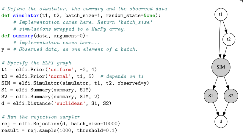
Figure 1: Baseline example for creating an ELFI model. Image taken from 1708.00707

All inference methods of ELFI are implemented following two conventions. First, their constructor follows the signature elfi.<Class name>(<output node>, *arg), where <output node> is the output node of the simulator-based model and *arg are the parameters of the method. Second, they provide a method elfi.<Class name>.sample(*args) for drawing samples from the approximate posterior.

3 Overview of the implementation

In this section, we express ROMC as an algorithm and then we present the general implementation principles.

3.1 Algorithmic view of ROMC

For designing an extendable implementation, we firstly define ROMC as a sequence of algorithmic steps. At a high level, ROMC can be split into the training and the inference part; the training part covers the steps for estimating the proposal regions and the inference part calculates the weighted samples. In Algorithm 1, that defines ROMC as an algorithm, steps 2-11 (before the horizontal line) refer to the training part and steps 13-18 to the inference part.

Algorithm 1 ROMC. Requires the prior $p(\boldsymbol{\theta})$, the simulator $M_{r}(\boldsymbol{\theta})$, number of optimization problems $n_{1}$, number of samples per region $n_{2}$, acceptance limit $\epsilon$

1:procedure ROMC

2:     for $i\leftarrow 1\textrm{ to }n_{1}$ do

3:         $\mathbf{u}_{i}\sim p(\mathbf{u})$ $\triangleright$ Draw nuisance variables

4:         Convert $M_{r}(\boldsymbol{\theta})$ to $g(\boldsymbol{\theta},\mathbf{u}=\mathbf{u}_{i})$ $\triangleright$ Define deterministic simulator

5:         $d_{i}(\boldsymbol{\theta})=d(g(\boldsymbol{\theta},\mathbf{u}=\mathbf{u}_{i}),\mathbf{y}_{0})$ $\triangleright$ Define distance function

6:         $\boldsymbol{\theta}_{i}^{*}=\text{argmin}_{\boldsymbol{\theta}}d_{i}$, $d_{i}^{*}=d_{i}(\boldsymbol{\theta}_{i}^{*})$ $\triangleright$ Solve optimization problem

7:         if $d^{*}_{i}>\epsilon$ then

8:              Go to 2 $\triangleright$ Filter solution

9:         end if

10:         Estimate $\hat{C^{i}_{\epsilon}}$ and define $q_{i}$ $\triangleright$ Estimate proposal area

11:         (Optional) Fit $\tilde{d}_{i}$ on $\hat{C^{i}_{\epsilon}}$ $\triangleright$ Fit surrogate model

12:

13:         for $j\leftarrow 1\textrm{ to }n_{2}$ do

14:              $\boldsymbol{\theta}_{ij}\sim q_{i}$, compute $w_{ij}$ as in Algorithm 3 $\triangleright$ Sample

15:         end for

16:     end for

17:     $\E_{p(\boldsymbol{\theta}|\mathbf{y_{0}})}[h(\boldsymbol{\theta})]$ as in eq. (11) $\triangleright$ Estimate an expectation

18:     $p_{d,\epsilon}(\boldsymbol{\theta})$ as in eq. (8) $\triangleright$ Evaluate the unnormalized posterior

19:end procedure

Training part

At the training (fitting) part, the goal is the estimation of the proposal regions $\hat{C^{i}_{\epsilon}}$, which expands to three mandatory tasks; (a) sample the nuisance variables $\mathbf{u}_{i}\sim p(\mathbf{u})$ for defining the deterministic distance functions $d_{i}(\boldsymbol{\theta})$ (steps 3-5), (b) solve the optimization problems for obtaining $\boldsymbol{\theta}_{i}^{*},d_{i}^{*}$ and keep the solutions inside the threshold $\epsilon$ (steps 6-9), and (c) estimate the bounding boxes $\hat{C}^{i}_{\epsilon}$ to define uniform distributions $q_{i}$ on them (step 10). Optionally, a surrogate model $\tilde{d}_{i}$ can be fitted for a faster inference phase (step 11).

If $d_{i}(\boldsymbol{\theta})$ is differentiable, using a gradient-based method is advised for obtaining $\boldsymbol{\theta}_{i}^{*}$ faster. In this case, the gradients $\nabla_{\boldsymbol{\theta}}d_{i}$ gradients are approximated automatically with finite-differences, if they are not provided in closed-form by the user. Finite-differences approximation requires two evaluations of $d_{i}$ for each parameter $\theta_{m},m\in\{1,\ldots,D\}$, which scales well only in low-dimensional problems. If $d_{i}(\boldsymbol{\theta})$ is not differentiable, Bayesian Optimization can be used as an alternative. In this scenario, the training part becomes slower due to fitting of the surrogate model and the blind optimization steps.

After obtaining the optimal points $\boldsymbol{\theta}^{*}_{i}$, we estimate the proposal regions. Algorithm 2 describes the line search approach for finding the region boundaries. The axes of each bounding box $\mathbf{v}_{m},m=\{1,\ldots,D\}$ are defined as the directions with the highest curvature at $\boldsymbol{\theta}_{i}^{*}$ computed by the eigenvalues of the Hessian matrix $\mathbf{H}_{i}$ of $d_{i}$ at $\boldsymbol{\theta}_{i}$ (step 1). Depending on the algorithm used in the optimization step, we either use the real distance $d_{i}$ or the Gaussian Process approximation $\hat{d}_{i}$. When the distance function is the Euclidean distance (default choice), the Hessian matrix can be also computed as $\mathbf{H}_{i}=\mathbf{J}_{i}^{T}\mathbf{J}_{i}$, where $\mathbf{J}_{i}$ is the Jacobian matrix of the summary statistics $\Phi(g(\boldsymbol{\theta},\mathbf{u}_{i}))$ at $\boldsymbol{\theta}_{i}^{*}$. This approximation has the computational advantage of using only first-order derivatives. After defining the axes, we search for the bounding box limits with a line step algorithm (steps 2-21). The key idea is to take long steps $\eta\_\text{start}$ until crossing the boundary and then take small steps backwards to find the exact boundary position.

Algorithm 2 Approximation $C^{i}_{\epsilon}$ with a bounding box $\hat{C^{i}_{\epsilon}}$; Requires: a model of distance $d_{i}(\boldsymbol{\theta})$, an optimal point $\boldsymbol{\theta}_{i}^{*}$, a number of refinements $K$, a step size $\eta\_\text{start}$, maximum iterations $M$ and a curvature matrix $\mathbf{H}_{i}$ ($\mathbf{J}_{i}^{T}\mathbf{J}_{i}$ or GP Hessian)

1:Compute eigenvectors $\mathbf{v}_{m}$ of $\mathbf{H}_{i}$ ($m=1,\ldots,D)$

2:for $m\leftarrow 1\textrm{ to }D$ do

3:     $\tilde{\boldsymbol{\theta}}\leftarrow\boldsymbol{\theta}_{i}^{*}$

4:     $k\leftarrow 0$

5:     $\eta\leftarrow\eta\_\text{start}$ $\triangleright$ Initialize $\eta$

6:     repeat

7:         $j\leftarrow 0$

8:         repeat

9:              $\tilde{\boldsymbol{\theta}}\leftarrow\tilde{\boldsymbol{\theta}}+\eta\ \mathbf{v}_{m}$ $\triangleright$ Large step size $\eta$.

10:              $j\leftarrow j+1$

11:         until $d(g(\tilde{\boldsymbol{\theta}},\mathbf{u}=\mathbf{u}_{i}),\mathbf{y_{0}})>\epsilon$ or $j\geq M$ $\triangleright$ Check distance or maximum iterations

12:         $\tilde{\boldsymbol{\theta}}\leftarrow\tilde{\boldsymbol{\theta}}-\eta\ \mathbf{v}_{m}$

13:         $\eta\leftarrow\eta/2$ $\triangleright$ More accurate region boundary

14:         $k\leftarrow k+1$

15:     until $k=K$

16:     if $\tilde{\boldsymbol{\theta}}=\boldsymbol{\theta}_{i}^{*}$ then $\triangleright$ Check if no step has been done

17:         $\tilde{\boldsymbol{\theta}}\leftarrow\tilde{\boldsymbol{\theta}}+\dfrac{\eta\_{\text{start}}}{2^{K}}\mathbf{v}_{m}$ $\triangleright$ Then, make the minimum step

18:     end if

19:     Set $\tilde{\boldsymbol{\theta}}$ as the positive end point along $\mathbf{v}_{m}$

20:     Run steps 3 - 18 for $\mathbf{v}_{m}=-\mathbf{v}_{m}$ and set $\tilde{\boldsymbol{\theta}}$ as the negative end point along $\mathbf{v}_{m}$

21:end for

22:Fit a rectangular box around the region end points and define $q_{i}$ as uniform distribution

Inference Part

The inference part includes one or more of the following three tasks; (a) sample from the posterior distribution $\boldsymbol{\theta}_{i}\sim p_{d,\epsilon}(\boldsymbol{\theta}|\mathbf{y_{0}})$ (Equation 10), (b) compute an expectation $\E_{\boldsymbol{\theta}|\mathbf{y_{0}}}[h(\boldsymbol{\theta})]$ (Equation 11) and/or (c) evaluate the unnormalized posterior $p_{d,\epsilon}(\boldsymbol{\theta}|\mathbf{y_{0}})$ (Equation 8). Sampling is performed by getting $n_{2}$ samples from each proposal distribution $q_{i}$. For each sample $\boldsymbol{\theta}_{ij}$, the distance function is evaluated for checking if it lies inside the acceptance region. Algorithm 3 defines the steps for computing a weighted sample. After we obtain weighted samples, computing the expectation is straightforward using Equation 11. Finally, evaluating the unnormalized posterior at a specific point $\boldsymbol{\theta}$ requires access to the distance functions $d_{i}$ and the prior distribution $p(\boldsymbol{\theta})$. Following Equation 8, we simply count for how many deterministic distance functions it holds that $d_{i}(\boldsymbol{\theta})<\epsilon$. It is worth noticing that for evaluating the unnormalized posterior, there is no need for solving the optimization problems and building the proposal regions.

Algorithm 3 Sampling. Requires a function of distance $d_{i}$, the prior distribution $p(\boldsymbol{\theta})$, the proposal distribution $q_{i}$

1:$\boldsymbol{\theta}_{ij}\sim q_{i}\forall i$ $\triangleright$ Sample parameters

2:for $i\leftarrow 1\textrm{ to }n_{1}$ do

3:     for $j\leftarrow 1\textrm{ to }n_{2}$ do

4:         if $d_{i}(\boldsymbol{\theta}_{ij})\leq\epsilon$ then $\triangleright$ Accept sample

5:              $w_{ij}=\frac{p(\boldsymbol{\theta}_{ij})}{q(\boldsymbol{\theta}_{ij})}$ $\triangleright$ Compute weight

6:              Store $(w_{ij},\boldsymbol{\theta}_{ij})$ $\triangleright$ Store weighted sample

7:         end if

8:     end for

9:end for

3.2 General implementation principles

Figure 2: Overview of the ROMC implementation. On the left side, we depict ROMC as a sequence of algotirhmic steps. On the right side, we present the functions that form our implementation; the green rectangles (starting with underscore) are the internal functionalities and the blue rectangles the publicly exposed API. This side-by-side illustration highlights that our implementation follows strictly the algorithmic view of ROMC.

The overview of our implementation is illustrated in Figure 2. Following Python naming principles, the methods starting with an underscore (green rectangles) represent internal (private) functions, whereas the rest (blue rectangles) are the methods exposed at the API. In Figure 2, it can be observed that the implementation follows Algorithm 1. The training part includes all the steps until the computation of the proposal regions, i.e., sampling the nuisance variables, defining the optimization problems, solving them, constructing the regions and fitting local surrogate models. The inference part comprises of evaluating the unnormalized posterior (and the normalized when is possible), sampling and computing an expectation. We also provide some utilities for inspecting the training process, such as plotting the histogram of the final distances or visualizing the constructed bounding boxes. Finally, in the evaluation part, we provide two methods for evaluating the inference; (a) computing the Effective Sample Size (ESS) of the samples and (b) measuring the divergence between the approximate posterior the ground-truth, if the latter is available.

Parallel version of ROMC

As discussed, ROMC has the significant advantage of being fully parallelisable. We exploit this fact by implementing a parallel version of the major fitting components; (a) solving the optimization problems, (b) constructing bounding box regions. We parallelize these processes using the built-in Python package multiprocessing. The specific package enables concurrency, using sub-processes instead of threads, for side-stepping the Global Interpreter (GIL). For activating the parallel version of the algorithm, the user simply has to set
elfi.ROMC(<output_node>, parallelize = True).

Simple one-dimensional example

For illustrating the functionalities we will use the following running example introduced by Ikonomov2019,

$$p(\theta)=\mathcal{U}(\theta;-2.5,2.5)$$ (13)

$$p(y|\theta)=\left\{\begin{array}[]{ll}\theta^{4}+u&\mbox{if }\theta\in[-0.5,0.5]\\ |\theta|-c+u&\mbox{otherwise}\end{array}\right.$$ (16)

$$u\sim\mathcal{N}(0,1)$$ (17)

The prior is a uniform distribution in the range $[-2.5,2.5]$ and the likelihood is defined at Equation 16. The constant $c$ is $0.5-0.5^{4}$ ensures that the PDF is continuous. There is only one observation $y_{0}=0$. The inference in this particular example can be performed quite easily without using a likelihood-free inference approach. We can exploit this fact for validating the accuracy of our implementation. At the following code snippet, we code the model at ELFI:

import elfi import scipy.stats as ss import numpy as np

def simulator(t1, batch_size = 1, random_state = None): c = 0.5 - 0.5**4 if t1 < -0.5: y = ss.norm(loc = -t1-c, scale = 1).rvs(random_state = random_state) elif t1 <= 0.5: y = ss.norm(loc = t1**4, scale = 1).rvs(random_state = random_state) else: y = ss.norm(loc = t1-c, scale = 1).rvs(random_state = random_state) return y

# observation y = 0

# Elfi graph t1 = elfi.Prior(’uniform’, -2.5, 5) sim = elfi.Simulator(simulator, t1, observed = y) d = elfi.Distance(’euclidean’, sim)

# Initialize the ROMC inference method bounds = [(-2.5, 2.5)] # bounds of the prior parallelize = False # True activates parallel execution romc = elfi.ROMC(d, bounds = bounds, parallelize = parallelize)

4 Implemented functionalities

At this section, we analyze the functionalities of the training, the inference and the evaluation part. Extended documentation for each method can be found in ELFI’s official documentation. Finally, we describe how a user may extend ROMC with its custom modules.

4.1 Training part

In this section, we describe the six functions of the training part:

>>> romc.solve_problems(n1, use_bo = False, optimizer_args = None)

This method (a) draws integers for setting the seed, (b) defines the optimization problems and (c) solves them using either a gradient-based optimizer (default choice) or Bayesian optimization (BO), if use_bo = True. The tasks are completed sequentially, as shown in Figure 2. The optimization problems are defined after drawing n1 integer numbers from a discrete uniform distribution $u_{i}\sim\mathcal{U}\{1,2^{32}-1\}$, where each integer $u_{i}$ is the seed passed to ELFI’s random simulator. The user can pass a Dict with custom parameters to the optimizer through optimizer_args. For example, in the gradient-based case, the user may pass optimizer_args = {"method": "L-BFGS-B", "jac": jac}, to select the "L-BFGS-B" optimizer and use the callable jac to compute the gradients in closed-form.

>>> romc.distance_hist(**kwargs)

This function helps the user decide which threshold $\epsilon$ to use by plotting a histogram of the distances at the optimal point $d_{i}(\boldsymbol{\theta}_{i}^{*}):\{i=1,2,\ldots,n_{1}\}$ or $\hat{d}_{i}^{*}$ in case use_bo = True. The function forwards the keyword arguments to the underlying pyplot.hist() of the matplotlib package. In this way the user may customize some properties of the histogram, e.g., the number of bins.

>>> romc.estimate_regions(eps_filter, use_surrogate = None, fit_models = False)

This method estimates the proposal regions around the optimal points, following Algorithm 2. The choice about the distance function follows the previous optimization step; if a gradient-based optimizer has been used, then estimating the proposal region is based on the real distance $d_{i}$. If BO is used, then the surrogate distance $\hat{d}$ is chosen. Setting use_surrogate=False enforces the use of the real distance $d$ even after BO. Finally, the parameter fit_models selects whether to fit local surrogate models $\tilde{d}$ after estimating the proposal regions.

The training part includes three more functions. The function romc.fit_posterior(args*) which is a syntactic sugar for applying .solve_problems() and .estimate_regions() in a single step. The function romc.visualize_region(i) plots the bounding box around the optimal point of the $i$-th optimization problem, when the parameter space is up to $2D$. Finally, romc.compute_eps(quantile) returns the appropriate distance value $d_{i=\kappa}^{*}$ where $\kappa=\lfloor quantile\cdot n\rfloor$ from the collection $\{d_{i}^{*}\},i=\{1,\ldots,n\}$ where $n$ is the number of accepted solutions. It can be used to automate the selection of the threshold $\epsilon$, e.g., eps=romc.compute_eps(quantile=0.9).

Example - Training part

In the following snippet, we put together the routines to code the training part of the running example.

# Training (fitting) part n1 = 500 # number of optimization problems seed = 21 # seed for solving the optimization problems use_bo = False # set to True for switching to Bayesian optimization

# Training step-by-step romc.solve_problems(n1 = n1, seed = seed, use_bo = use_bo) romc.theta_hist(bins = 100) # plot hist to decide which eps to use

eps = .75 # threshold for the bounding box romc.estimate_regions(eps = eps) # build the bounding boxes

romc.visualize_region(i = 2) # for inspecting visually the bounding box

# Equivalent one-line command # romc.fit_posterior(n1 = n1, eps = eps, use_bo = use_bo, seed = seed)

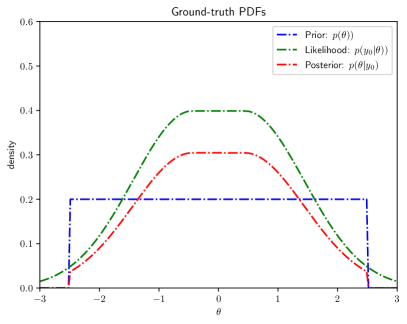
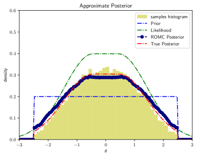
Figure 3: Histogram of distances and visualization of a specific region.

4.2 Inference part

In this section, we describe the four functions of the inference part:

>>> romc.sample(n2)

This is the basic functionality of the inference, drawing $n_{2}$ samples for each bounding box region, giving a total of $k\cdot n_{2}$ samples, where $k<n_{1}$ is the number of the optimal points remained after filtering. The samples are drawn from a uniform distribution $q_{i}$ defined over the corresponding bounding box and the weight $w_{i}$ is computed as in Algorithm 3.

The inference part includes three more function. The function romc.compute_expectation(h) computes the expectation $\E_{p(\boldsymbol{\theta}|\mathbf{y_{0}})}[h(\boldsymbol{\theta})]$ as in Equation 11. The argument h can be any python Callable. The method romc.eval_unnorm_posterior(theta, eps_cutoff = False) computes the unnormalized posterior approximation as in Equation 3. The method
romc.eval_posterior(theta, eps_cutoff = False) evaluates the normalized posterior estimating the partition function $Z=\int p_{d,\epsilon}(\boldsymbol{\theta}|\mathbf{y_{0}})d\boldsymbol{\theta}$ using Riemann’s integral approximation. The approximation is computationally feasible only in a low-dimensional parametric space.

Example - Inference part

In the following code snippet, we use the inference utilities to (a) get weighted samples from the approximate posterior, (b) compute an expectation and (c) evaluate the approximate posterior. We also use some of ELFI’s built-in tools to get a summary of the obtained samples. For romc.compute_expectation(), we demonstrate its use to compute the samples mean and the samples variance. Finally, we evaluate romc.eval_posterior() at multiple points to plot the approximate posterior of Figure 3. We observe that the approximation is quite close to the ground-truth.

# Inference part seed = 21 n2 = 50 romc.sample(n2 = n2, seed = seed)

# visualize region, adding the samples now romc.visualize_region(i = 1)

# Visualize marginal (built-in ELFI tool) weights = romc.result.weights romc.result.plot_marginals(weights = weights, bins = 100, range = (-3,3))

# Summarize the samples (built-in ELFI tool) romc.result.summary() # Method: ROMC # Number of samples: 19300 # Parameter Mean 2.5# theta: -0.012 -1.985 1.987

# compute expectation exp_val = romc.compute_expectation(h = lambda x: np.squeeze(x)) print("Expected value : # Expected value: -0.012

exp_var = romc.compute_expectation(h = lambda x: np.squeeze(x)**2) print("Expected variance: # Expected variance: 1.120

# eval unnorm posterior print("# 58.800

# check eval posterior print("# 0.289

4.3 Evaluation part

The method romc.compute_ess() computes the Effective Sample Size (ESS) as $\frac{(\sum_{i}w_{i})^{2}}{\sum_{i}w_{i}^{2}}$, which is a useful quantity to measure how many samples actually contribute to an expectation. For example, in an extreme case of a big population of samples where only one has big weight, the ESS is much smaller than the samples population.

The method romc.compute_divergence(gt_posterior, bounds, step, distance) estimate the divergence between the ROMC approximation and the ground truth posterior. Since the estimation is performed using Riemann’s approximation, the method can only work in low dimensional spaces. The method can be used for evaluation in synthetic examples where the ground truth is accessible. In a real-case scenarios, where it is not expected to have access to the ground-truth posterior, the user may set the approximate posterior obtained with any other inference approach for comparing the two methods. The argument step defines the step used in the Riemann’s approximation and the argument distance can be either "Jensen-Shannon" or "KL-divergence".

# Evaluation part res = romc.compute