Optical two-mode squeezed interferometer for enhanced chip-integrated quantum-metrology

Abstract

In this work we analyze the possibility to use two-mode squeezed light to improve the performance of existing sensor technology with the focus on its miniaturization. Based on a general four-wave mixing (FWM) Hamiltonian, we formulate simple linearized equations that describe the FWM process below threshold and can be used to analyze the squeezing quality between the generated optical signal and idler modes. For a possible realization, we focus on the chip-integrated generation using micro-ringresonators and the impact of the design and the pump light on the squeezing quality is shown with the derived equations. With this we analyze the usage in quantrum metrology and analyze the application of two-mode squeezed light in a Mach-Zehnder interferometer (MZI) and for a deeper understanding and motivation also in the application of a Sagnac-interferometer. Due to the impact of losses in these use cases, we show that the main usage is for small and compact devices, which can lead to a quantum improvement up to a factor of ten in comparison of using only classical light. This enables the use of small quantum-enhanced sensors with a comparable performance to larger classical sensors.

I Introduction

Quantum-metrology has the potential to use completely new sensing principles, to enable new use cases and to increase the sensitivity of existing measurement technology Nawrocki (2019). The main motivation for quantum-metrology in comparison to its classical counterpart is that in theory, quantum-sensors are not shot noise limited anymore with $1/\sqrt{N}$, instead they can achieve the Heisenberg limit with $1/N$ where $N$ denotes the number of probes which can be for example the number of photons or the number of measurement repetitions Giovannetti et al. (2006, 2011). However, in reality this is very challenging to achieve. The reason is that quantum states like single-photons are heavily affected by losses and decoherence effects which makes it difficult building a Heisenberg-limited quantum sensor Dorner et al. (2009); Rafal Demkowicz-Dobrzański and Marcin Jarzyna and Jan Kołodyński (2015). Despite this, there are applications which make use of a quantum enhancement like the famous example of gravitational-wave detection. Thereby, single-mode squeezed-light is used to increase the phase-sensitivity of a huge interferometer to detect extremely small signals caused by gravitational waves et al. (2016); Vahlbruch et al. (2010).
In this work, we show the potential using two-mode squeezed light generated by FWM for quantum-enhanced optical interferometry. The FWM process is utilized in many applications like for the creation of frequency-combs for sensing and communication Chang et al. (2020); Fortier and Baumann (2019) or for squeezed state generation for optical quantum-computing J. M. Arrazola et al. (2021). We want to use it to generate two-mode squeezed light for sensing applications. The main focus lays on a realistic quantum-metrology platform that is realizable with existing technology in photonic-integrated circuits. To do so, we discuss a system that is shown in figure 5. It exists of laser light that is coupled inside two optical waveguides and one pumps a ringresonator to generate two-mode squeezed light via FWM which is sent into a sensor region together with additional coherent light from the other light path. Using multi-mode interferometers (MMI) as beamsplitter, a MZI can be realized.
We see big potential for quantum-metrology in the miniaturization of existing sensor concepts. Therefore, we show a theoretical example for a quantum-enhanced Sagnac-interferometer that has the potential to miniaturize existing concepts and thus, can be used for a wide range of applications. The potential for gyroscopes using quantum states has already been discussed in the past and it has been shown that, in principle, they can get close to the Heisenberg limit Kolkiran and Agarwal (2007). Based on this idea, there are recent concepts that discuss theoretical realizations De Leonardis et al. (2020); Jiao and An (2022); Grace et al. (2020) and it has already been demonstrated using a large setup with entangled single-photons Fink et al. (2019). Although they all show interesting results, neither of them provides a detailed discussion about the realistic physical potential and the equations required to perform a proper design which is realizable with typical losses and fabrication technologies in combination with the expected system performance.
In the following sections, we discuss how to generate two-mode squeezed light using a ringresonator, how to determine the outra-cavity mode using input-output theory and how to use it to calculate the sensing limit in a lossy MZI. Finally, we show that the quantum-enhancement can improve the sensor performance by an order of magnitude. However, due to the waveguide losses, squeezed light is only useful for a compact or low-loss sensor concept which leads to an advantage as a quantum-enhanced chip-integrated optical gyroscope.

II Four-Wave Mixing

FWM is a well-known non-linear optical process which describes the effect of two pump modes $a_{p}(t)$ beeing absorbed by a material with a significant third-order susceptibility coefficient $\chi^{(3)}$ while emitting two new modes which are called signal $a_{s}(t)$ and idler $a_{i}(t)$ with energy conservation $\omega_{i}+\omega_{s}=2\omega_{p}$. For simplicity we write $a_{i}(t):=a_{i}$ for the time dependent operator. Following Vernon and Sipe (2015), the FWM Hamiltonian inside of a resonator and with only one pump mode $a_{p}$ can be given in the rotating-wave approximation as

$$H_{\mathrm{FWM}}= \hbar(\omega_{p}a_{p}^{\dagger}a_{p}+\omega_{s}a_{s}^{\dagger}a_{s}+\omega_{i}a_{i}^{\dagger}a_{i})$$ (1)

$$+\hbar g(a_{p}a_{p}a_{s}^{\dagger}a_{i}^{\dagger}+a_{p}^{\dagger}a_{p}^{\dagger}a_{s}a_{i})$$

$$+\frac{\hbar g}{2}a_{p}^{\dagger}a_{p}^{\dagger}a_{p}a_{p}$$

$$+2\hbar g(a_{s}^{\dagger}a_{p}^{\dagger}a_{s}a_{p}+a_{i}^{\dagger}a_{p}^{\dagger}a_{i}a_{p})$$

with the nonlinear gain $g$, which is further discussed in appendix A. The first line corresponds to the cavity resonance frequencies $\omega_{p}$, $\omega_{s}$, $\omega_{i}$ and second line to the desired FWM process which represents the non-linear interaction in which two pump modes are either absorbed or generated in exchange with one signal and one idler mode. The self-phase modulation (SPM) is shown in the third line where the pump induces a non-linear shift on its own which is well-known as the duffing effect. The last line corresponds to the cross-phase modulation (XPM) in which the pump mode induces a frequency shift to the signal and idler mode.
Note that in equation 1 the SPM and XPM effect caused by the signal and idler modes are neglected. The reason is that we focus in this work on the below threshold operation and thus, the signal and idler correspond to low-power modes. Additionally, only one signal and idler mode is present in equation 1 due to the below thresehold operation in which only one mode is generated. Multi modes are important above the threshold which corresponds to the frequency-comb generation. Since we assume a well implemented control loop, we will neglect the SPM and XPM effect in the following. Using this, a linearization of the Hamiltonian is performed assuming the pump to be close to constant with the complex amplitude inside of the cavity $\langle a_{p}\rangle=\alpha_{cv}$ which leads to the following Hamiltonian

$$H_{\mathrm{FWM},\mathrm{lin}}=\hbar(\omega_{s}a_{s}^{\dagger}a_{s}+\omega_{i}a_{i}^{\dagger}a_{i})+\frac{i\hbar}{2}(\sigma a_{s}^{\dagger}a_{i}^{\dagger}-\sigma^{*}a_{s}a_{i})$$ (2)

with introducing the injection parameter $\sigma=2g\cdot\alpha_{cv}^{2}$ which can have, similar as in Vernon and Sipe (2015), a detuning and a certain phase with

$$\sigma=\overline{\sigma}\cdot e^{-i(\Delta_{\sigma}t-\phi_{\sigma})}$$ (3)

and the FWM detuning $\Delta_{\sigma}=\omega_{s}+\omega_{i}-2\omega_{p}$. This detuning should be zero for the best performance and can be achieved with dispersion engineering of the waveguide geometry Fujii and Tanabe (2020).

III Input-Output-Theory

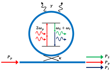
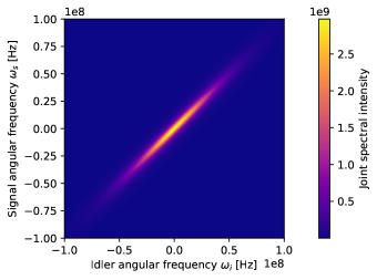
Figure 1: Left: Ringresonator which is used to generate squeezed light via FWM. A pump mode $P_{p}$ is pumped over the coupling parameter $\kappa$ inside the cavity in which a strong pump field generates a signal and idler mode which couple out of the cavity. Losses appear are accounted for by $\gamma$. Right: Joint spectral intensity between the signal and idler mode calculated using equation 49 with $T=0.01$, $n_{eff}=1.801$, $n_{g}=2.10087$, $\alpha=0.23$ $\frac{1}{\mathrm{m}}$, $L=2\pi\cdot 220\cdot 10^{-6}$ m, $\omega_{p}=1550\cdot 10^{-6}$ m, $n_{2}=2.4\cdot 10^{-19}$ $\mathrm{m}^{2}/\mathrm{W}$, $A_{eff}=1.05564\cdot 10^{-12}$ $\mathrm{m}^{2}$, $\sigma=0.998\cdot\sigma_{th}$

To be able to determine the performance of possible systems using the generated two-mode squeezed states, it is required to solve the Hamiltonian of equation 2 and to determine equations for the expectation values of the output modes. Therefore, we first introduce the desired resonator structure that is shown in figure 1. It exists of a straight waveguide connected to a ring-shaped waveguide that acts as resonator. A pump mode inside the straight waveguide is coupled with evanescent waveguide-coupling which can be described by the coupling rate $\kappa$ to the resonator and builds up an enhanced cavity pump field that is described by the complex amplitude $\alpha_{cv}$ and can generate signal and idler modes via FWM. Since we focus on a microscopic device, the integrated resonator is the preferred structure and it enables that less pump power $P_{P}$ is required to achieve FWM and to generate squeezed states.
Due to imperfections of the waveguide and mostly due to scattering, energy is lost inside of the cavity which is described by the loss rate $\gamma$. Both rates $\kappa$ and $\gamma$ describe the photon rate that leaves or enters the cavity due to the respective effect. Note that the cavity mode is attenuated due to a detuning from the resonance frequency $\omega_{p}$ and due to losses through $\gamma$ and $\kappa$, while it is also driven through $\kappa$. Using these decay rates, the coherent pump inside of the cavity can be described with the simple equation of motion of a driven cavity which can be given as

$$\frac{d}{dt}\alpha_{cv}=-i\omega_{p}\alpha_{cv}-\frac{\gamma+\kappa}{2}\alpha_{cv}+\sqrt{\kappa}\alpha_{p}$$ (4)

with $\alpha_{p}$ being the light pumped inside of the cavity which can have a phase $\alpha_{p}=\overline{\alpha}_{p}\cdot e^{i\phi_{a_{p}}}$. This equation is solved by performing the Fourier-transformation which leads to

$$\alpha_{cv}=\frac{\sqrt{\kappa}\alpha_{p}}{(\gamma+\kappa)/2-i(\omega-\omega_{p})}$$ (5)

with the detuning of the laser to the resonance wavelength $\Delta_{p}=\omega-\omega_{p}$ which is an important part if effects like SPM or optical bi-stability are considered. The physical relation to the given parameters $\kappa$, $\gamma$ and $\alpha_{p}$ in dependency on the ring-design variations is explained in more detail in appendix B.

III.1 Quantum Langevin equation

The outra-cavity expectation values of the signal and idler modes are derived with the quantum Langevin approach. We start with the definition of the interaction Hamiltonian which describes the interaction between the intra-cavity and outra-cavity modes. For the ringresonator in figure 1, there exist two bath-modes which couple to the cavity modes, but not with each other. This is once the bath inside of the straight waveguide $b_{\kappa}$ which couples over $\kappa$ and the bath outside of the ring $b_{\gamma}$ which couples over $\gamma$ and corresponds to the waveguide losses. It is well known that the bath couplings can be described in dependency of the decay rates with $\sqrt{\kappa}b_{s/i,\kappa}$ and $\sqrt{\gamma}b_{s/i,\gamma}$ Collett and Gardiner (1984); Gardiner and Collett (1985); Scully and Zubairy (1997). This leads to the following interaction Hamiltonian.

$$H_{\mathrm{int}}=\hbar\cdot(\sqrt{\kappa}a_{s}^{\dagger}b_{s,\kappa}+\sqrt{\gamma}a_{s}^{\dagger}b_{s,\gamma}+\sqrt{\kappa}a_{i}^{\dagger}b_{i,\kappa}+\sqrt{\gamma}a_{i}^{\dagger}b_{i,\gamma})+\mathrm{h.c.}$$ (6)

Note that if the wavelength separation between the signal and idler is significant, it is important to differ between coupling and loss rates of each and both rates would require the corresponding indices.
Since we want to keep it general applicable, it is important to assume the case that beside the pump mode also a coherent part of the signal and idler is pumped into the ring-resonator. Thus, the waveguide bath mode can be split into a fluctuation part $b_{\kappa,f}$ and a static part $b_{\kappa,st}$ with

$$b_{\kappa}=b_{\kappa,f}+b_{\kappa,st}$$ (7)

in which we set the static part to the complex amplitude $\langle b_{\kappa,st}\rangle=\alpha_{i/s}=\overline{\alpha}_{i/s}\cdot e^{i\phi_{a_{i/s}}}$. Using this, it is possible to derive the quantum Langevin equation of motion in the Heisenberg picture of the intra-cavity modes in dependency of the bath modes which can be derived as following Lam (2007)

$$\frac{da_{s/i}}{dt}=-\frac{i}{\hbar}[a_{s/i},H_{\mathrm{FWM},\mathrm{lin}}+H_{\mathrm{int}}].$$ (8)

This leads to the following equation of motion and its complex conjugate

$$\frac{da_{s/i}}{dt}= -i\omega_{s/i}a_{s/i}+\frac{\sigma}{2}a_{i/s}^{\dagger}-\frac{\gamma}{2}a_{s/i}-\frac{\kappa}{2}a_{s/i}+\sqrt{\kappa}\alpha_{s/i}+\sqrt{\kappa}b_{s/i,\kappa}+\sqrt{\gamma}b_{s/i,\gamma}$$ (9)

$$\frac{da_{s/i}^{\dagger}}{dt}= i\omega_{s/i}a_{s/i}^{\dagger}+\frac{\sigma^{*}}{2}a_{i/s}-\frac{\gamma}{2}a_{s/i}^{\dagger}-\frac{\kappa}{2}a_{s/i}^{\dagger}+\sqrt{\kappa}\alpha_{s/i}^{*}+\sqrt{\kappa}b_{s/i,\kappa}^{\dagger}+\sqrt{\gamma}b_{s/i,\gamma}^{\dagger}.$$ (10)

The boundary condition describing the output bath operator $b_{out}$ and thus, the output field for a vacuum input has already been derived in Collett and Gardiner (1984); Gardiner and Collett (1985), where it has been proved that it is also valid for a coherent input. Thus, using equation 7 as the definition for the input bath we can define the boundary condition as following

$$b_{s/i,in}=\sqrt{\kappa}a_{s/i}-b_{s/i}-\alpha_{s/i},$$ (11)

where $b_{s/i}:=b_{s/i,out}$ corresponds to the output mode. This leads to the following equations of motion describing the intra-cavity field using the output bath operator

$$\frac{da_{s/i}}{dt}= -i\omega_{s/i}a_{s/i}+\frac{\sigma}{2}a_{i/s}^{\dagger}-\frac{\gamma}{2}a_{s/i}-\frac{\kappa}{2}a_{s/i}-\sqrt{\kappa}b_{s/i,out}+\sqrt{\gamma}b_{s/i,\gamma}$$ (12)

$$\frac{da_{s/i}^{\dagger}}{dt}= i\omega_{s/i}a_{s/i}^{\dagger}+\frac{\sigma^{*}}{2}a_{i/s}-\frac{\gamma}{2}a_{s/i}^{\dagger}-\frac{\kappa}{2}a_{s/i}^{\dagger}-\sqrt{\kappa}b_{s/i,out}^{\dagger}+\sqrt{\gamma}b_{s/i,\gamma}^{\dagger}.$$ (13)

For a more compact description, the equations 9, 10 and 13, 12 can be given in matrix notation as following for the input and output bath operators.

$$\frac{d}{dt}\mathbf{A} =(\mathbf{K}+\frac{\kappa}{2}\mathbf{I_{4}})\mathbf{A}+\sqrt{\kappa}\mathbf{B_{\kappa}}+\sqrt{\gamma}\mathbf{B_{\gamma}}+\sqrt{\kappa}\mathbf{F_{c}},$$ (14)

$$\frac{d}{dt}\mathbf{A} =(\mathbf{K}-\frac{\kappa}{2}\mathbf{I_{4}})\mathbf{A}-\sqrt{\kappa}\mathbf{B_{out}}+\sqrt{\gamma}\mathbf{B_{\gamma}}.$$ (15)

Thereby, $\mathbf{I_{4}}$ is the identity matrix with a dimension of four and we use the following notations for the other matrices.

$$\mathbf{B_{\kappa}}=\left(\begin{array}[]{c}b_{s,\kappa}\\ b_{s,\kappa}^{\dagger}\\ b_{i,\kappa}\\ b_{i,\kappa}^{\dagger}\end{array}\right),\mathbf{B_{\gamma}}=\left(\begin{array}[]{c}b_{s,\gamma}\\ b_{s,\gamma}^{\dagger}\\ b_{i,\gamma}\\ b_{i,\gamma}^{\dagger}\end{array}\right),\mathbf{B_{out}}=\left(\begin{array}[]{c}b_{s}\\ b_{s}^{\dagger}\\ b_{i}\\ b_{i}^{\dagger}\end{array}\right),$$ (28)

$$\mathbf{A}=\left(\begin{array}[]{c}a_{s}\\ a_{s}^{\dagger}\\ a_{i}\\ a_{i}^{\dagger}\end{array}\right),\mathbf{F_{c}}=\left(\begin{array}[]{c}\alpha_{s}\\ \alpha_{s}^{*}\\ \alpha_{i}\\ \alpha_{i}^{*}\end{array}\right),$$ (37)

$$\mathbf{K}=\left(\begin{matrix}-i\omega_{s}-\frac{\gamma}{2}&0&0&\frac{\sigma}{2}\\ 0&i\omega_{s}-\frac{\gamma}{2}&\frac{\sigma^{*}}{2}&0\\ 0&i\frac{\sigma}{2}&-i\omega_{i}-\frac{\gamma}{2}&0\\ \frac{\sigma^{*}}{2}&0&0&i\omega_{i}-\frac{\gamma}{2}\\ \end{matrix}\right).$$ (38)

Since these are all linear equations, it is possible to perform the Fourier-transformation. This leads to the following matrix notations of the equation of motion in the frequency domain

$$\mathbf{A(\omega)}[\mathbf{\Omega}+\frac{\kappa}{2}\mathbf{I_{4}}-\mathbf{K}] =\sqrt{\kappa}\mathbf{B_{\kappa}}+\sqrt{\gamma}\mathbf{B_{\gamma}}+\sqrt{\kappa}\mathbf{F_{c}},$$ (39)

$$\mathbf{A(\omega)}[\mathbf{\Omega}-\frac{\kappa}{2}\mathbf{I_{4}}-\mathbf{K}] =-\sqrt{\kappa}\mathbf{B_{out}}+\sqrt{\gamma}\mathbf{B_{\gamma}},$$ (40)

where $\mathbf{\Omega}$ is the frequqency matrix with

$$\mathbf{\Omega}=\left(\begin{matrix}-i\omega&0&0&0\\ 0&i\omega&0&0\\ 0&0&-i\omega&0\\ 0&0&0&i\omega\\ \end{matrix}\right)$$ (41)

This is now a simple matrix system which can be re-arranged to eliminate the intra-cavity mode and to determine the output mode of the system using only the bath modes and the system operators with

$$\mathbf{B_{out}}=- \frac{1}{\sqrt{\kappa}}\Bigl{[}[\mathbf{\Omega}-\frac{\kappa}{2}\mathbf{I_{4}}-\mathbf{K}][\mathbf{\Omega}+\frac{\kappa}{2}\mathbf{I_{4}}-\mathbf{K}]^{-1}\cdot(\sqrt{\kappa}\mathbf{B_{\kappa}}+\sqrt{\gamma}\mathbf{B_{\gamma}}+\sqrt{\kappa}\mathbf{F_{c}})-\sqrt{\gamma}\mathbf{B_{\gamma}}\Bigr{]}.$$ (42)

Note that by subtracting $\mathbf{\Omega}$ by $\mathbf{K}$, we introduce the detunings of the signal and idler mode with $\Delta_{i}=\omega-\omega_{i}$ and $\Delta_{s}=\omega-\omega_{s}$, which are zero for a perfect cavity design and FWM phase-matching. By using equation 42, it is possible to determine the expectation values of the output modes. To achieve this, we make usage of the expectation definitions of the bath modes which are in vacuum states with Zoller and Gardiner (1997); Wiseman and Milburn (2009)

$$\langle b\rangle = \langle b^{\dagger}\rangle=\langle bb\rangle=\langle b^{\dagger}b\rangle=0$$

$$\langle bb^{\dagger}\rangle = \delta(t).$$ (43)

For the resulting expectation values, we define a helpful function that appears more often in the following equations

$$\Xi=(4\Delta_{i}\Delta_{s}-\sigma^{2})^{2}+4\Gamma^{2}(\Delta_{i}^{2}+\Delta_{s}^{2})+\Gamma^{4}.$$ (44)

with the total losses of the cavity modes $\Gamma=\gamma+\kappa$. One important equation is the output signal photon number of the fluctuation with $\alpha_{i}=\alpha_{s}=0$ which is solved to

$$\langle b_{s}^{\dagger}b_{s}\rangle=\frac{4\sigma^{2}\kappa\Gamma}{\Xi-2\sigma^{2}\Gamma^{2}}\overset{\Delta_{i}=\Delta_{s}=0}{=}\frac{4\sigma^{2}\kappa\Gamma}{(\Gamma^{2}-\sigma^{2})^{2}}.$$ (45)

This equation diverges for $\sigma=\Gamma:=\sigma_{th}$ which corresponds to the threshold of the FWM process. The other results of the expectation values are given in the appendix C.

III.2 Mean-field theory

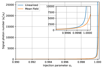
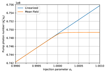
Figure 2: Left: Signal photon number $\langle a_{p}^{\dagger}a_{p}\rangle$ for the linearized approach (blue) and MF (orange) Right: Pump photon number $\langle a_{p}^{\dagger}a_{p}\rangle$ for the linearized approach (blue) and MF (orange). For both the following values are used: $\Delta_{i}=\Delta_{s}=\Delta_{p}=0$, $X=0.01$, $n_{eff}=1.801$, $n_{g}=2.10087$, $\alpha=0.23$ $\frac{1}{\mathrm{m}}$, $L=2\pi\cdot 220\cdot 10^{-6}$ m, $\omega_{p}=1550\cdot 10^{-6}$ m, $n_{2}=2.4\cdot 10^{-19}$ $\mathrm{m}^{2}$/W, $A_{e}ff=1.05564\cdot 10^{-12}$ $\mathrm{m}^{2}$

The divergence in equation 45 is not physical and thus, it is necessary to know the range of $\sigma$ in which the derived equations are valid as well as to validate our linearized Hamiltonian approach. For this, we determine the results of the expectation values using the mean-field theory (MF) which assumes that the pump mode is uncorrelated of the signal and idler. It is a more realistic view since the pump mode still appears in the Hamiltonian. Knowing that the MF is not perfect as well, it has been shown that it is very accurate below the threshold Degenfeld-Schonburg et al. (2016) and thus, we can use it to validate the range of $\sigma$.
Based on the Hamiltonian from equation 1, we derive the following driven Hamiltonian for the FWM process neglecting SPM and XPM

$$H_{\mathrm{FWM,MF}}= \omega_{i}a_{i}^{\dagger}a_{i}+\omega_{s}a_{s}^{\dagger}a_{s}+\omega_{p}a_{p}^{\dagger}a_{p}+ig(a_{p}a_{p}a_{s}^{\dagger}a_{i}^{\dagger}-a_{p}^{\dagger}a_{p}^{\dagger}a_{s}a_{i})+\sqrt{\kappa}\alpha_{p}a_{p}^{\dagger}+\sqrt{\kappa}\alpha_{p}^{*}a_{p}.$$ (46)

Using this Hamiltonian and the linearized one in equation 2, we derive a master equation for each of the intra-cavity modes with

$$\frac{\delta\rho}{\delta t}=-i[H_{\mathrm{MF}},\rho]+\sum_{j={i,s,p}}\Gamma_{j}[a_{j}\rho a_{j}^{\dagger}-\frac{1}{2}(a_{j}^{\dagger}a_{j}\rho+\rho a_{j}^{\dagger}a_{j})]$$ (47)

$$\frac{\delta\rho}{\delta t}=-i[H_{\mathrm{lin}},\rho]+\sum_{j={i,s}}\Gamma_{j}[a_{j}\rho a_{j}^{\dagger}-\frac{1}{2}(a_{j}^{\dagger}a_{j}\rho+\rho a_{j}^{\dagger}a_{j})].$$ (48)

In comparison with the MF master equation, the pump mode does not appear in the linearized one which is the biggest difference. Each of the master-equations leads to a coupled non-linear equation system which can be solved using a numerical approach. Since the results should be realistic, numerical values of a real system are used. For this an optical silicon nitride (Si3N4) waveguide with the height of $800$ nm, a width of $1.2$ $\mu$m and a bend radius of $220$ $\mathrm{\mu}$m was simulated using a mode solver at a wavelength of $\lambda=1.5$ $\mu$m. This dimension is in the range where squeezing generation with a ringresonator has already been demonstrated Vaidya et al. (2020). The nonlinear index is approximated to be $2.4\cdot 10^{-19}$ $\frac{\mathrm{m}^{2}}{W}$ based on Ikeda et al. (2008) which leads to a $g=1.5$ Hz. Losses of $1\frac{\mathrm{dB}}{\mathrm{m}}$ and a ring transmission of $0.01$ are assumed which lead to $\gamma=38.3$ MHz and $\kappa=1208$ MHz.
The results for the signal photon number $\langle a_{s}^{\dagger}a_{s}\rangle$ and the pump photon number $\langle a_{p}^{\dagger}a_{p}\rangle$ is shown in figure 2 over the normalized injection parameter $\sigma_{n}=\sigma/\sigma_{th}$ which is exactly one at the threshold. While for MF $\langle a_{p}^{\dagger}a_{p}\rangle$ is determined using the master equation, the linearized approach is solved using equation 5. It can be clearly seen that pump depletion appears at $\sigma_{c}=1$ for MF while $\langle a_{p}^{\dagger}a_{p}\rangle$ rises for the linearized approach. For $\langle a_{s}^{\dagger}a_{s}\rangle$ it can be seen that the linearized approach diverges at $\sigma_{n}=1$, while the MF solution is still rising reasonably. The MF and the linearized solution split shortly before the threshold which shows that the linearized approach can be used till the threshold. Tolerating an error of 5 %, $\sigma$ is valid from a value of zero up to $0.99895\cdot\sigma_{th}$

III.3 Outra-cavity squeezing

With the results above, the squeezing of the outra-cavity modes can be analyzed. For this work it is of special interest how the two-mode squeezing of the outra-cavity signal and idler modes behaves in dependency of the system parameters. One way to analyze the squeezed light is the joint spectral intensity $\Phi$ which can be solved as

$$\Phi=\langle b_{s}^{\dagger}b_{i}^{\dagger}b_{s}b_{i}\rangle=\frac{4\kappa^{2}\sigma^{2}(\Xi+6\sigma^{2}\Gamma^{2})}{\Xi-2\sigma^{2}\Gamma^{2}}.$$ (49)

It can be interpreted as the two-dimensional probability distribution and is an indication for the correlation between the two modes over the frequency Zielnicki et al. (2018). The result of $\Phi$ is shown in figure 1 over the signal and idler frequency with the same values for the geometry as above and a $\sigma_{n}=0.995$. It is interesting that the spectrum is squeezed with a high correlation and broadband in the case of a symmetric detuning between the signal and the idler. This behaviour can change depended on the physical parameters .
Another important feature of squeezed light is the quadrature operator which allows the analysis of the noise behaviour with Walls and Milburn (2008)

$$X_{Q}=\frac{(b_{s}+b_{i})e^{i\phi_{LO}}+(b_{s}^{\dagger}+b_{i}^{\dagger})e^{-i\phi_{LO}}}{\sqrt{2}}$$ (50)

with the local oscillator (LO) phase $\phi_{LO}$. In experiments this phase can be used to change the measured signal from low-noise or squeezing at $\phi_{LO}=\pi/2$ to the high-noise or anti-squeezing $\phi_{LO}=0$ case. Thereby, the outra-cavity light is mixed with a coherent local oscillator laser with a certain phase to realize the desired quadrature operator. Of special interest is the variance of the quadrature to identify the noise of the two-mode squeezed light which is defined as Walls and Milburn (2008)

$$V=\Delta X_{Q}=\langle X_{Q}^{2}\rangle-\langle X_{Q}\rangle^{2}\xrightarrow{\alpha_{i/s}=0}\langle X^{2}_{Q}\rangle.$$ (51)

If no coherent part is present, the expectation values of the single modes are zero. In the case with zero detuning, the following equations are determined for the squeezed and anti-squeezed variance

$$V_{\phi_{LO}=0}=\frac{\Gamma^{2}+\sigma^{2}}{(\Gamma+\sigma)^{2}}+\frac{2\sigma(\kappa-\gamma)}{(\Gamma+\sigma)^{2}}$$ (52)

$$V_{\phi_{LO}=\pi/2}=\frac{\Gamma^{2}+\sigma^{2}}{(\Gamma-\sigma)^{2}}-\frac{2\sigma(\kappa-\gamma)}{(\Gamma-\sigma)^{2}}.$$ (53)

The results of equation 51 over the phase $\phi_{LO}$ are shown in figure 3 with the same geometry values from above. Thereby, the different colors represent various pump powers with $\sigma_{n}$ and it can be seen that with rising power, the squeezing improves while the anti-squeezing increases. A squeezing of approximately $-15.02$ dB can be achieved for the defined limit $\sigma_{n}=0.99895$. This is close to the value with less pump $\sigma_{n}=0.95$ with $-15.01$ dB which is about $-12$ dB lower than vacuum and thus, good noise reduction can be already achieved with a power close to the threshold. However, the difference for the anti-squeezing is significantly larger with $65.46$ dB for $\sigma_{n}=0.99895$ and $31.68$ dB for $\sigma_{n}=0.95$.
For the design it is important to know how it effects the squeezing. In this case, the two main parameters are the decay rates $\kappa$ and $\gamma$ which can be tuned by the ring design. The influence for different ratios between $\kappa$ and $\gamma$ are shown in figure 4. The best squeezing can be achieved for the case $\kappa>\gamma$ which is also known as overcoupling, since more light couples in and out of the ring than is lost due to losses. For the so called critical coupling case in which both coupling rates are equal with $\kappa=\gamma$, the squeezing decreases and for the undercoupling case with $\kappa<\gamma$ the variance is similar to the vacuum noise. This matches the results of other works and shows the importance of a proper cavity design Chembo (2016).

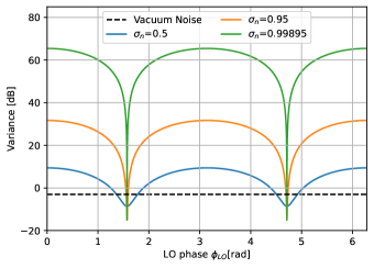
Figure 3: Variance of the two-mode squeezed light calculated using equation 51 over the LO phase with a variation of $\sigma_{n}$.

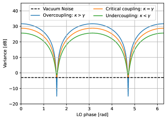
Figure 4: Variance of the two-mode squeezed light calculated using equation 51 over the LO phase with a variation of $\kappa$ and $\gamma$. The variations are achieved with $\alpha_{L}=0.23$ 1/m for overcoupling, $\alpha_{L}=7.28$ 1/m for critical coupling and $\alpha_{L}=23.04$ 1/m for undercoupling while $\sigma_{n}$ is constant at 0.95.

IV Mach-Zehnder interferometer

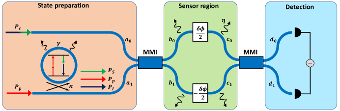
Figure 5: Schematic of a MZI which exists of a state preparation (orange), sensor region (green) and a detection stage (blue).

The main goal of this work is to show the potential of two-mode squeezed states generated by FWM in a sensor application that is build in the form of a MZI and to determine the sensing limit. The desired system is shown in figure 5 and is split into a part for the state preparation, the sensor region and the detection.
At the state preparation, pump light $P_{p}$ with the amplitude $\alpha_{p}$ and coherent light $P_{c}$ with the amplitude $\alpha_{c}$ is coupled into the chip with using $P_{p}$ to pump the ringresonator. The generated outra-cavity signal and idler mode, which correspond to the state $a_{1}$ and $P_{c}$ as the state $a_{0}$, are sent into the MZI via a MMI, which acts as a beamsplitter (BS). Afterwards, the states arrive in the sensor region which applies a symmetric phase-shift (PS) to them. The BS and PS can be defined as following

$$\mathbf{BS}=\left(\begin{matrix}\frac{1}{\sqrt{2}}&\frac{1}{\sqrt{2}}\\ \frac{1}{\sqrt{2}}&-\frac{1}{\sqrt{2}}\end{matrix}\right),\mathbf{PS}=\left(\begin{matrix}e^{i\frac{\phi}{2}}&0\\ 0&e^{-i\frac{\phi}{2}}\end{matrix}\right).$$ (54)

The sensor region is typically the largest area of the system and thus, it is important to consider losses to model a realistic application. This is done in the standard way using a BS that couples a vacuum mode $b_{v}$ inside of the system while out-coupling the system mode Rafal Demkowicz-Dobrzański and Marcin Jarzyna and Jan Kołodyński (2015). Therefore, we introduce the efficiency $\eta$ related to the mode power which is one for the lossless case. The loss must be applied on each path of the MZI with two uncorrelated vacuum modes and can be described as following.

$$l=\sqrt{\eta}b_{0/1}+\sqrt{1-\eta}b_{0/1,v}.$$ (55)

This is discussed in more details and with the physical relation in appendix D. The expectation values from equation 43 are valid for the calculation with the vacuum modes. After the sensor region another BS follows and the modes at the detection stage $\mathbf{D}=(d_{0}\>d_{1})^{\top}$ can be determined in dependency of the input modes $\mathbf{A}=(a_{0}\>a_{1})^{\top}$ with

$$\mathbf{D}=\mathbf{BS}\cdot\left[\left(\begin{matrix}\sqrt{\eta}\\ \sqrt{\eta}\end{matrix}\right)\cdot\mathbf{PS}\cdot\mathbf{BS}\cdot\mathbf{A}+\left(\begin{matrix}\sqrt{1-\eta}b_{v,0}\\ \sqrt{1-\eta}b_{v,1}\end{matrix}\right)\right].$$ (56)

Afterwards, the output modes are detected and further processed with some electronic readout circuits. For the detection scheme, we use the commonly used intensity difference detection which is defined as

$$\mathrm{ID}=d_{0}^{\dagger}d_{0}-d_{1}^{\dagger}d_{1}.$$ (57)

It is obvious that in reality losses appear at each stage for example at the detector and the signal processing which should be modeled using equation 55 Bachor and Ralph (2004). As shown in Rafal Demkowicz-Dobrzański and Marcin Jarzyna and Jan Kołodyński (2015) it is sufficient to focus on the losses within the optical system because these are the most significant ones and the other losses can be merged to this loss.

V Quantum-sensing limit

To determine the performance and the quantum-enhancement of the system, it is necessary to determine the noise of the measurement operator. In general the minimum detectable phase change inside of the MZI $\Delta\phi$ can be evaluated using error propagation Braunstein and Caves (1994); Rafal Demkowicz-Dobrzański and Marcin Jarzyna and Jan Kołodyński (2015)

$$\Delta\phi=\frac{\sqrt{\Delta\mathrm{ID}}}{|\delta\langle\mathrm{ID}\rangle/\delta\phi|}$$ (58)

with $\Delta\mathrm{ID}=\langle\mathrm{ID}^{2}\rangle-\langle\mathrm{ID}\rangle^{2}$. Therefore, the previous derived expectation values are required. Since in equation 58 higher order expectation values appear, we use the helpful cumulant expansion which decreases the order of an operator $\mathbf{X}$ with Kubo (1962)

$$\langle X_{1}X_{2}...X_{n}\rangle=\sum_{p\in P(I)/I}(|p|-1)!(-1)^{|p|}\prod_{B\in p}\langle\prod_{i\in B}X_{i}\rangle$$ (59)

and $P(I)/I$ being the set of all operators excluding $I$. Using this, it is possible to determine the noise in the MZI and thus, to find out the minimal detectable phase change of the system.
For a MZI with intensity difference detection, it is shown in appendix E that the optimal phase sensitivity is at the working point of $\phi_{opt}=\frac{\pi}{2}$. The phase sensitivity with only a coherent input under lossy conditions at $\phi_{opt}$ is determined with the following expression

$$\Delta\phi_{\mathrm{C}}=\frac{1}{\sqrt{\eta}\alpha_{c}}$$ (60)

and corresponds to the case for which $P_{p}$ is not used to pump the ringresonator and thus, without squeezed-light generation. Equation 60 scales as good as the shot-noise limit (SNL) with $1/\alpha_{c}$ for the lossless case and with losses it is slightly worse. For the case of using $P_{p}$ to pump the ringresonator to generate squeezed light and mixing this with coherent light, the phase sensitivity at $\phi_{opt}$ can be expressed as

$$\Delta\phi_{\mathrm{S}}=\frac{\sqrt{\eta^{2}\alpha_{c}^{2}(\Gamma-\sigma)^{2}(\Gamma^{2}+\sigma(2\gamma-6\kappa)+\sigma^{2})+\eta\alpha_{c}^{2}(\Gamma^{2}-\sigma^{2})^{2}+8\kappa\sigma^{2}\Gamma\eta}}{(\Gamma^{2}-\sigma^{2})|\eta\alpha_{c}^{2}-\frac{8\eta\sigma^{2}\kappa\Gamma}{(\Gamma^{2}-\sigma^{2})^{2}}|}.$$ (61)

It can be seen that two pole points can appear. One at $\sigma=\Gamma$ which is however not allowed withing the valid range for $\sigma$ and the second one if the number of squeezed photons matches the number of coherent photons. However, this only appears for rather small values of $\alpha_{c}$. Thus, $\alpha_{c}$ should be chosen large enough which is in most applications already the case with small pump powers less than micro-watt. This behaviour is analyzed in more detail in appendix E.
For the optimal conditions, with no losses and thus with $\eta=1$, $\gamma=0$ and a coherent pump with $\alpha_{c}>10^{4}$, the phase sensitivity can be approximated to the following expression

$$\Delta\phi_{\mathrm{S,opt}}\approx\frac{\sqrt{2}}{\alpha_{c}}\frac{\kappa-\sigma}{\kappa+\sigma}.$$ (62)

Depending on the squeezing quality described by the values for $\kappa$ and $\sigma$, an improvement in scaling over equation 60 and the SNL can be achieved by up to three orders of magnitude within the valid range of $\sigma$. However, equation 62 is challenging to reach in a real world application, since losses will appear.
To identify how well both systems perform in a more realistic and lossy setting, it is necessary to also analyze the SNL of the system. This SNL is calculated with the total number of photons inside of the MZI. However, as indicated in the state preparation in figure 5, the pump power that is required to generate the two-mode squeezed light is included as well in the SNL. This results in the following equation for the SNL

$$\Delta\phi_{\mathrm{SNL}}=\frac{1}{\sqrt{N}}=\frac{1}{\sqrt{\langle d_{0}^{\dagger}d_{0}\rangle+\langle d_{1}^{\dagger}d_{1}\rangle+\alpha_{p}^{2}}}.$$ (63)

with the number of photons in the system $N$. The addition of $\alpha_{p}$ is required since the pump is not modeled in the outra-cavity expectation values. In our opinion it is important to include $a_{p}$ in equation 63. The reason is that it only makes sense to use squeezed light if there is a better system performance by using $a_{p}$ for pumping a ringresonator or any non-linear material for the squeezed-light generation, instead of using it directly for sensing.
To analyze this behaviour in more detail, the phase sensitivity is shown over the input power in figure 6 with coherent input, squeezed light mixed with coherent light and the SNL for comparison. It can be seen that the phase sensitivity for a coherent input improves with increasing power by the same scaling as the SNL, which is as expected. Even with a higher loss and thus, a lower $\eta$, the scaling is similar and just the performance decreases slightly by a factor of $1/\sqrt{\eta}$.
For the squeezed-part with low input power, the phase sensitivity is way higher and thus worse than the coherent and SNL part. The reason is that far below the threshold, the pump light required for pumping the ringresonator $\alpha_{p}$ does not contribute to the sensing performance but to the SNL as indicated by equation 63. Instead, at low pump power, only a weak two-mode squeezed light is available for sensing with increasing performance for growing power which corresponds to a larger $\sigma_{n}$. The pump power is increased close to threshold with $\sigma_{n}=0.99895$ which corresponds to a power of 14.12 mW. However, the performance using only the squeezed light is way worse than using coherent light. With the squeezed light only, a phase sensitivity of about $0.008$ can be achieved.
This is because the pump power is constant at the input power of $\sigma_{n}=0.99895$ and the coherent power $P_{c}$ is increased afterwards. This significantly improves the performance and the phase sensitivity of the squeezed light mixed with coherent light surpasses the coherent only and the SNL performance. However, the impact of losses on squeezed light is way larger than on coherent light which is in agreement with Schnabel (2017). Despite this fact, the scaling over input power is still better for the lossy case of the squeezed light mixed with coherent light and thus, it surpasses the lossy coherent performance and would also improve further compared to the SNL. This is shown in the zoomed part of figure 6.
To achieve a real quantum-enhancement and an advantage compared to classical light, it is necessary that a low threshold can be achieved. The reason is that the scaling of the squeezed light mixed with coherent light is superior than using only coherent light. However, this advantage only applies if the threshold allows the squeezed light sensitivity to surpass the coherent sensitivity at a reasonable power. The threshold can be changed by adapting the design, as shown in equation 45, or by using a material with a high-nonlinear susceptibility.

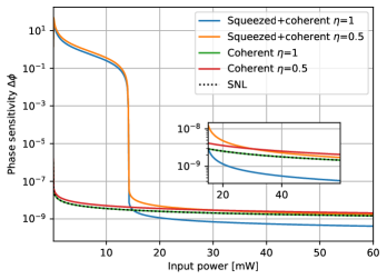
Figure 6: Phase sensitivity over the input power for squeezed light mixed with coherent light (blue lossless and orange with losses), coherent light (green lossless and red with losses) and the SNL (black dotted). For the calculation are the following values used: $\Delta_{i}=\Delta_{s}=\Delta_{p}=0$, $T=0.01$, $n_{eff}=1.801$, $n_{g}=2.10087$, $\alpha=0.23$ $\frac{1}{\mathrm{m}}$, $L=2\pi\cdot 220\cdot 10^{-6}$ m, $\omega_{p}=1550\cdot 10^{-6}$ m, $n_{2}=2.4\cdot 10^{-19}$ $\mathrm{m}^{2}$/W, $A_{e}ff=1.05564\cdot 10^{-12}$ $\mathrm{m}^{2}$

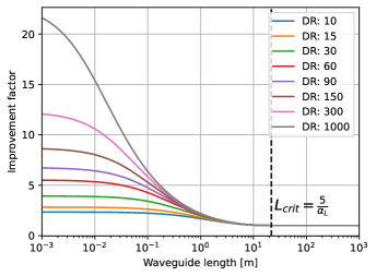
Figure 7: Improvement factor evaluated with equation 64 over the waveguide length of the sensor region for different decay ratios.

The applied PS as well as the losses are not fixed in real life applications but depend on the scale of the sensor region. Examples for this are Sagnac interferometers in which a larger sensing area leads to a an stronger phase shift or Raman measurements in which the interaction length between the light and the molecules enhances the signal. However, with a large area, the losses rise as well with equation 75. To analyze the performance improvement of squeezed light compared to using coherent light, we define the improvement factor $\mathrm{I}$ which is just the ratio between $\Delta\phi_{c}$ and $\Delta\phi_{s}$ with

$$\mathrm{I}=\frac{\Delta\phi_{c}}{\Delta\phi_{s}},$$ (64)

since a smaller $\Delta\phi$ is better. Since the squeezing depends on the decay rates $\kappa$ and $\gamma$ as it is shown above in figure 4, equation 64 is analyzed for a variation of the ratio of both which we define as the decay ratio with

$$\mathrm{DR}=\frac{\kappa}{\gamma}.$$ (65)

However, note that with increasing $\mathrm{SR}$ also the threshold rises as shown in equation 45. The results of equation 64 are shown in figure 7. It can be seen that for short lengths and rising decay ratios, the improvement factor rises as well which proves the quantum advantage. The improvement factor for a short length can be approximated with

$$\mathrm{I}_{\mathrm{Length}\rightarrow 0}=10.218\cdot\mathrm{ln}\biggl{(}\mathrm{DR}+143.47\biggr{)}-49.816.$$ (66)

In contrast to this is the behaviour with long lengths where $\mathrm{I}$ reaches one. This can be explained by the fact that losses increase with length and the squeezed state is highly susceptible to them. After a certain length most of the squeezing is lost and no advantage can be achieved. We call this length the critical length which depends on the losses and can be approximated as

$$L_{crit}=\frac{5}{\alpha_{L}}$$ (67)

with the losses $\alpha_{L}$ which are explained in more detail in appendix B. This behaviour demonstrates our starting motivation, that the quantum-enhancement shows its strength for chip-integrated applications which mostly consist of short lenghts and low-loss applications. Dependent on the use case, it can be useful to decrease the size of a sensor and to increase the sensitivity using two-mode squeezed light.

VI Conclusion

In this work we analyzed the generation of two-mode squeezed light in a cavity and its application for sensing in a MZI which can improve the sensitivity compared to classical sensing for low-loss applications. We started with a linearized Hamiltonian for the FWM process and derived the expecation values of the outra-cavity signal and idler modes via the quantum Langevin input-output theory. They are used to determine the squeezing behaviour of the two-mode squeezed light and to give a support to design a cavity for the desired squeezing behaviour. Additionally, we used the derived equations to calculate the minimum detectable phase change inside of a MZI and it has been shown that squeezed light mixed with coherent light can surpass the phase sensitivity of the SNL.
However, for a real use case it is important to tune the threshold by design and material choice in a reasonable region, where the improved slope of the squeezed light can show its full potential. Furthermore, we showed that the losses of a system limits the usability of two-mode squeezed light. The reason is that squeezed light is very loss sensitive and after a certain length of the sensor region, most of the squeezing is lost and no improvement can be achieved compared to a classical sensor. However, if the sensor region is small, two-mode squeezed light can significantly increase the performance by more than a factor of ten. We showed that this improvement factor depends on the decay ratio and thus, on the design of the cavity. This leads to an optimization problem between a desired decay ratio and a low threshold. If both is chosen reasonable, then the quantum enhancement can be beneficial.
In summary we think that this can lead to more compact sized sensors which can have the same sensitivity at a small size as with a larger sensor region due to the quantum enhancement. It is important to note that squeezed light can improve the performance of many various optical sensor concepts and, as shown in this work, especially for interferometer based sensor principles that are nowadays already available to manufacture and to use.

Appendix A Gain of the four-wave mixing process

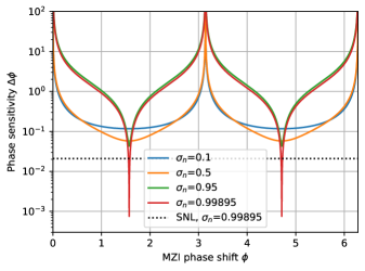
Figure 8: Phase sensitivity over the MZI phase shift $\phi$ with a weak coherent pump $\alpha_{c}=10$ and for different $\sigma_{n}$.

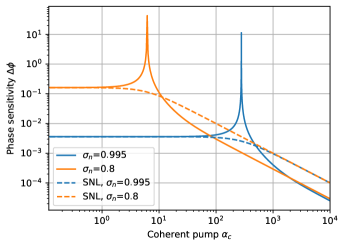
Figure 9: Phase sensitivity over the coherent pump $\alpha_{c}$ at MZI phase shift $\phi=\pi/2$ for different $\sigma_{n}$.

Based on the derivation in Vernon and Sipe (2015) the gain of the FWM-process inside of a ring-resonator can be given in the following expression

$$g=\frac{\hbar(\omega_{p}^{2}\omega_{s}\omega_{i})^{1/4}v_{g}^{2}\gamma_{NL}}{L}$$ (68)

with the group velocity $v_{g}$, the length of the resonator $L$ and the nonlinear waveguide parameter $\gamma_{NL}$ which is given by Agrawal (2013)

$$\gamma_{NL}=\frac{\omega_{p}n_{2}}{cA_{eff}}$$ (69)

with the nonlinear refractive index $n_{2}$ which can be described as

$$n_{2}=\frac{3\chi^{(3)}}{4\varepsilon_{0}cn_{eff}^{2}}$$ (70)

and the effective refractive index $n_{eff}$. Since $n_{2}$ is mostly used in the literature we give our final gain as following

$$g=\frac{\hbar\omega_{p}(\omega_{p}^{2}\omega_{s}\omega_{i})^{1/4}v_{g}^{2}n_{2}}{cA_{eff}L}\approx\frac{\hbar\omega_{p}v_{g}^{2}n_{2}}{cA_{eff}L}.$$ (71)

Note that the derivations slightly differ from each other as in Hoff et al. (2015). Since it is derived with some approximations, one can only be correct with a value for the gain by performing measurements.

Appendix B Physical relation to the parameters

For a practical realization of a system it is very important to know the physical relation of the operators and how they behave with the structure dimensions. The parameter for the design of the ringresonator are the decay rate $\gamma$ and the coupling rate $\kappa$. They describe how much light decays via the respective effect at each round trip time which is describes as following for a laser pulse

$$t_{round}=\frac{n_{eff}L}{c}$$ (72)

with the effective refractive index of the waveguide $n_{eff}$, the length of the ring $L$ and the speed of light $c$. At each round trip a certain part of the light couples out of the ring-resonator into the connected waveguide by a certain percentage and this is described by the cross coupling $X$ which takes the values $0\leq X\leq 1$. All the light is transmitted at a value of one and no light at a value of zero. Thus, the coupling rate can be defined as the light that is coupled out per round trip

$$\kappa=\frac{X}{t_{round}}=\frac{Xc}{n_{eff}L}.$$ (73)

Additionally, at each round-trip a certain part of the light is scattered away caused by for example scattering on rough waveguide walls. In general, the optical power in lossy photonic chip integrated waveguides over a length $L$ can be described by the following equation Hunsperger (2002)

$$P(L)=P_{0}\cdot e^{-\alpha_{L}L}$$ (74)

with the optical waveguide losses $\alpha_{L}$ in the units of $m^{-1}$. To model the losses now in dependency of the waveguide losses and together with the knowledge that $P(L)\leq P_{0}$, we simply define it as the relative power change with a value of one for no losses and a value zero for maximum losses

$$\eta=1-\frac{P_{0}-P(L)}{P_{0}}=e^{-\alpha_{L}L}.$$ (75)

Based on this we can define the decay rate per round trip time as following

$$\gamma=\frac{1-\eta}{t_{round}}=\frac{(1-e^{-\alpha_{L}L})c}{n_{eff}L}.$$ (76)

Another important physical parameter is the complex amplitude of a coherent pump. It is known that this can be described as

$$\alpha_{p}=\sqrt{\frac{P}{\hbar\omega_{p}}}$$ (77)

with the pump power $P$ and the freequency of the light $\omega_{p}$ and is proportional to a photon flux.

Appendix C Outra-cavity expectation values

In the following, the results of the calculated outra-cavity expectation values are given and determined based on equation 42. Thereby, the expectation values are split into a static $\langle b_{st}\rangle$ and a fluctuating part $\langle b_{f}\rangle$ with the total expectation value being $\langle b_{out}\rangle=\langle b_{f}\rangle+\langle b_{st}\rangle$. However, only the signal modes and some cross products between the signal and idler modes are given. The reason is that due to symmetry, the idler results can be simply achieved by a swap of the index in the equations. Based on them, all desired expectation values can be determined.

C.1 Fluctuating results

For the fluctuating results with $\alpha_{i/s}=0$, all first order expectation values are zero $\langle b_{s,f}\rangle=\langle b_{s,f}^{\dagger}\rangle=0$ as well as the following second order values: $\langle b_{s,f}b_{s,f}\rangle=\langle b_{s,f}^{\dagger}b_{s,f}^{\dagger}\rangle=\langle b_{i,f}b_{s,f}^{\dagger}\rangle=\langle b_{s,f}b_{i,f}^{\dagger}\rangle=\langle b_{s,f}^{\dagger}b_{i,f}\rangle=\langle b_{i,f}^{\dagger}b_{s,f}\rangle=0$. The relevant results are given in the following:

$$\langle b_{i,f}b_{s,f}\rangle=\frac{-2\kappa\sigma(4\Delta_{i}\Delta_{s}-2i\Gamma(\Delta_{i}+\Delta_{s})-\Gamma^{2}-\sigma^{2})}{\Xi-2\sigma^{2}\Gamma^{2}}$$ (78)

$$\langle b_{i,f}^{\dagger}b_{s,f}^{\dagger}\rangle=\frac{-2\kappa\sigma(4\Delta_{i}\Delta_{s}+2i\Gamma(\Delta_{i}+\Delta_{s})-\Gamma^{2}-\sigma^{2})}{\Xi-2\sigma^{2}\Gamma^{2}}$$ (79)

The equation for the photon number $\langle b_{s,f}^{\dagger}b_{s,f}\rangle$ is already given in equation 45. Note that the other expectation values can be determined either due to the relation $\langle b_{s,f}b_{s,f}^{\dagger}\rangle=1+\langle b_{s,f}^{\dagger}b_{s,f}\rangle$ or due to symmetries like $\langle b_{i,f}^{\dagger}b_{s,f}^{\dagger}\rangle=\langle b_{s,f}^{\dagger}b_{i,f}^{\dagger}\rangle$. Thus, all expectation values for the fluctuating results can be determined with the few given equations.

C.2 Static results

For the static results each expectation value is unequal zero. However, to determine each expectation value only the following two equation 80 and 81 are required and the rest can be determined using symmetries.

$$\langle b_{s,st}\rangle=\frac{\alpha_{s}(\kappa^{2}+\sigma^{2}-\gamma^{2}-4\Delta_{i}\Delta_{s}-2i[\Delta_{i}(\gamma-\kappa)+\Delta_{s}\Gamma])-2\alpha_{i}\kappa\sigma}{4\Delta_{i}\Delta_{s}+2i\Gamma(\Delta_{i}-\Delta_{s})+\Gamma^{2}-\sigma^{2}}$$ (80)

$$\langle b_{s,st}^{\dagger}\rangle=\frac{\alpha_{s}(\kappa^{2}+\sigma^{2}-\gamma^{2}-4\Delta_{i}\Delta_{s}+2i[\Delta_{i}(\gamma-\kappa)+\Delta_{s}\Gamma])-2\alpha_{i}\kappa\sigma}{4\Delta_{i}\Delta_{s}-2i\Gamma(\Delta_{i}-\Delta_{s})+\Gamma^{2}-\sigma^{2}}$$ (81)

The other equations can be simply determined by multiplication

$$\langle b_{s,st}b_{s,st}^{\dagger}\rangle=\langle b_{s,st}\rangle\cdot\langle b_{s,st}^{\dagger}\rangle$$ (82)

$$\langle b_{s,st}^{\dagger}b_{s,st}\rangle=\langle b_{s,st}^{\dagger}\rangle\cdot\langle b_{s,st}\rangle$$ (83)

$$\langle b_{i,st}b_{s,st}\rangle=\langle b_{i,st}\rangle\cdot\langle b_{s,st}\rangle$$ (84)

or by changing the index between the signal and idler modes. In this way, all static expectation values can be determined.

Appendix D Waveguide losses in the MZI

Losses in quantum systems are mostly modeled using a beamsplitter description with an efficiency $\eta$ as following

$$\mathbf{LM}=\left(\begin{matrix}\sqrt{\eta}&\sqrt{1-\eta}\\ \sqrt{1-\eta}&-\sqrt{\eta}\end{matrix}\right)$$ (85)

Thereby, $\eta$ is in the range $0\leq\eta\leq 1$ with a value of one for no losses and is described by the equation 75. It is important to note that while parts of the waveguide mode $a$ is lost, vacuum is coupled into the system Bachor and Ralph (2004). The resulting mode can be determined with

$$l=\sqrt{\eta}a+\sqrt{1-\eta}b_{v}$$ (86)

an the vacuum bath mode $b_{v}$. The part that couples out of the waveguide can be described by 85. However, only the mode in the waveguide is important and the lost mode is ignored.

Appendix E MZI Phase sensitivity

The phase sensitivity for the MZI in figure 5 is calculated using equation 58 and is shown in figure 8. Thereby, the case that a weak coherent pump is sent in $P_{c}$ and a different pump is sent in $P_{p}$ to pump the ringresonator and to generate two-mode squeezed light via FWM. It can be seen that the sensitivity diverges for a phase of $\phi=0$ while it reaches the optimum at $\phi=\frac{\pi}{2}$ and $\phi=\frac{3\pi}{2}$ which should be the preferred working points for a sensing application. It can be seen that the phase sensitivity improves the closer $\sigma_{n}$ is to the threshold.
In comparison, also the SNL using equation 63 with $\alpha_{p}=0$ is shown for the case with the strongest $\sigma_{n}=0.99895$. As expected, the phase-sensitivity for the same pump surpasses the SNL by more than a magnitude. This shows that two-mode squeezed light can be used for quantum-enhanced metrology which matches other work Steuernagel and Scheel (2004).
Additionally, it is interesting to analyze the pole-point that results out of equation 61. Therefore, equation 61 is plotted over the coherent pump $\alpha_{c}$ for two different $\sigma_{n}$ values in figure 9. It can be seen that for both $\sigma_{n}$ values, a pole-position is visible which appears for lower $\sigma_{n}$ at lower $\alpha_{c}$. This is similar to the results of other works Ataman (2019). The phase sensitivity is constant till this pole-position and afterwards it improves with rising $\alpha_{c}$. For both $\sigma_{n}$ the improvement is similar after the pole-position while the higher $\sigma_{n}$ surpasses the lower one. However, for $\alpha_{c}$ values that are lower than at the pole-point the phase sensitivity is the same as the SNL. The position of this pole position is exactly if the number of photons in the coherent pump $\langle a_{c}^{\dagger}a_{c}\rangle$ matches the number of photons of the squeezed states $\langle a_{s}^{\dagger}a_{s}\rangle+\langle a_{i}^{\dagger}a_{i}\rangle$. This matches the results of Pezzé and Smerzi (2008) and shows that a high coherent pump is required to achieve an improved scaling compared to the SNL.