Variational method for learning Quantum Channels via Stinespring Dilation on neutral atom systems

Abstract

The state $|\psi(t)\rangle$ of a closed quantum system evolves under the Schrödinger equation, where the reversible evolution of the state is described by the action of a unitary operator $U(t)$ on the initial state $|\psi_{0}\rangle$, i.e. $|\psi(t)\rangle=U(t)|\psi_{0}\rangle$. However, realistic quantum systems interact with their environment, resulting in non-reversible evolutions, described by Lindblad equations. The solution of these equations give rise to quantum channels $\Phi_{t}$ that describe the evolution of density matrices according to $\rho(t)=\Phi_{t}(\rho_{0})$, which often results in decoherence and dephasing of the state. For many quantum experiments, the time until which measurements can be done might be limited, e.g. by experimental instability or technological constraints. However, further evolution of the state may be of interest. For instance, to determine the source of the decoherence and dephasing, or to identify the steady state of the evolution. In this work, we introduce a method to approximate a given target quantum channel by means of variationally approximating equivalent unitaries on an extended system, invoking the Stinespring dilation theorem. We report on an experimentally feasible method to extrapolate the quantum channel on discrete time steps using only data on the first time steps. Our approach heavily relies on the ability to spatially transport entangled qubits, which is unique to the neutral atom quantum computing architecture. Furthermore, the method shows promising predictive power for various non-trivial quantum channels. Lastly, a quantitative analysis is performed between gate-based and pulse-based variational quantum algorithms.

I Introduction

In the current noisy intermediate-scale quantum (NISQ) era Preskill (2018), quantum computers suffer from noise and are limited in their computational power. Nevertheless, these NISQ systems are useful for specific, well-designed tasks Arute et al. (2019). The currently predominant algorithms are variational quantum algorithms (VQAs) that aim to construct a unitary operation that minimizes a prescribed loss function. Certain VQAs have shown proof of concept for small dimensional problems with various hardware choices of qubits Kandala et al. (2017); Hempel et al. (2018); Aspuru-Guzik and Walther (2012); O’Brien et al. (2018); Arute et al. (2020). Another application of NISQ-era quantum computers is quantum simulation. Here, the goal is to simulate the behavior of a closed quantum system evolving under the Schrödinger equation, by mimicking the Hamiltonian of the target system. This results in a unitary evolution that fully describes the dynamics of the system.

On the other hand, many quantum systems of interest consist of a subsystem interacting with an environment, a so-called open quantum system, e.g. photonic devices, fermionic lattices Del Re et al. (2020), ion collisions, quark-gluon plasmas Jong et al. (2021) or even a NISQ quantum computer Wang et al. (2023). This interaction leads to non-unitary evolutions described by the Lindblad equation Brasil et al. (2013) (see Eq. (1)), generally portraying dissipation in the form of dephasing and decoherence. Evolution operators associated to this equation are called quantum channels—the open system equivalent of unitary operators. In this paper, we propose a novel quantum channel VQA to approximate the evolution of these open systems, which we call the target system.

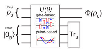
Figure 1: Schematic representation of a quantum channel VQA using ancilla qubits. Both gate- and pulse-based methods can be used for the Stinespring unitary approximation.

Approach.

Our method first considers a number of computational qubits on the quantum computer, depending on the dimensionality of the Hilbert space in which the target quantum channel is described. In order to capture the behavior of the environment, this Hilbert space is extended by introducing a number of ancilla qubits based on the Stinespring dilation theorem (see Sec. II) Foss-Feig et al. (2021). The method then variationally learns a unitary operator on this extended system (computational + ancilla qubits)—henceforth called the Stinespring unitary—based on input measurement data on the computational qubits. The Stinespring unitary is traced out over the ancilla qubits (environment) to provide an approximation of the target quantum channel, see Fig. 1.

By repeatedly moving away the old ancilla qubits and applying the Stinespring unitary on the computational system and new ancillas, the quantum channel can be repeated, resulting in approximations of the target quantum channel at discrete time steps. Because of its ability to coherently move around qubits Bluvstein et al. (2022), a neutral atom quantum computing system is especially well-suited for initializing a new set of ancilla qubits.

Relation to previous work.

Several other works have been previously performed on quantum channel approximations using quantum computers and the Stinespring dilation theorem Schlimgen et al. (2022); Hu et al. (2020); Head-Marsden et al. (2021); Hu et al. (2022); Jong et al. (2021); Foss-Feig et al. (2021); Wang et al. (2023). Our method differs from these previous approaches in the sense that no prior knowledge is required on the Lindblad equation jump operators (see Eq. (1)) and the method fully relies on measurement data on the target system, such as can be provided by an experiment. Moreover, we introduce the inclusion of input data at multiple discrete time steps and the steady state. Lastly, ours is the first to consider a pulse-based method for quantum channel approximation. Furthermore, we also note parallels between our approach and other ancilla qubit methods for quantum channel simulation including quantum Zeno dynamics Patsch et al. (2020), unitary decomposition Schlimgen et al. (2021), and imaginary time evolution Del Re et al. (2020); McArdle et al. (2019).

The layout of this paper is as follows. Sec. II describes quantum channels and the Stinespring dilation theorem. Sec. III details the newly developed quantum channel VQA. Sec. IV describes how the algorithm is readily tailored towards execution on a NISQ neutral atom quantum computing system. In Sec. V, we show initial results of our quantum channel approximation method and compare gate- and pulse-based methods.

II Quantum Channels & Stinespring Dilation

A system of interest will always, albeit limited, interact with its environment. This results in an open quantum system undergoing decoherence and dephasing Hornberger (2009) (see Fig. 2), which can no longer be represented using pure states $|\psi\rangle$, but requires the use of density matrices $\rho$, henceforth called states. The evolution of such an open quantum system is described by the Lindblad equation Brasil et al. (2013); Weinberg (2016)

$$\partial_{t}\rho=-i\left[H(t),\rho\right]+\sum_{k}\gamma_{k}A_{k}\rho A_{k}^{\dagger}-\frac{1}{2}\gamma_{k}\left\{A_{k}^{\dagger}A_{k},\rho\right\},$$ (1)

with $H(t)$ the original Hamiltonian acting on the system of interest, $A_{k}$ the jump operators with corresponding decay rates $\gamma_{k}$, that characterize the interactions with the environment, and $[\cdot,\cdot]$ and $\{\cdot,\cdot\}$ respectively the commutator and anti-commutator. Solutions to the Lindblad equation are described by a quantum channel $\Phi_{t}$ acting on states as

$$\rho(t)=\Phi_{t}(\rho_{0}).$$ (2)

A quantum channel has the following properties Holevo (2019):

• $\Phi_{t}$ is linear;

• $\Phi_{t}$ is completely positive (i.e. $I_{n}\otimes\Phi_{t}$ is positive for every $n$);

• $\Phi_{t}$ is trace preserving.

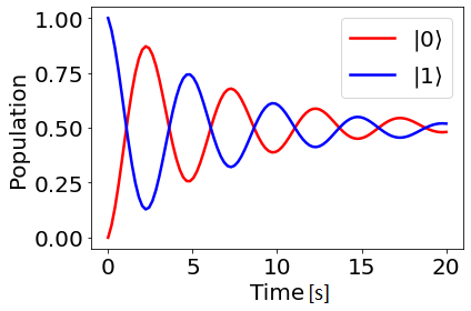
Figure 2: Example of quantum channel behavior showing populations for single qubit Rabi oscillation with $\Omega=0.4\pi$ Hz, $A=|1\rangle\langle 0|$ and $\gamma=0.15$ Hz decay.

Because of the high dimensionality of the Hilbert spaces on which quantum channels act, it is not computationally feasible to simulate these channels on classical computers. Therefore, we propose a method which utilizes the highly dimensional computational space inherent to quantum computers. The qubits of an ideal quantum computer form a closed system and evolve only under unitary transformations. As a result, it is impossible to mimic a non-unitary quantum channel acting on a $2^{m}$ dimensional space by using a quantum computer with only $m$ qubits. In dilation theory, operators on a Hilbert space $A$ are extended as projections of operators that act on a larger Hilbert space $A\otimes B$. The new operator is then called a dilation and can have more favorable properties than the original operator Shalit (2020). For this work, we employ the Stinespring dilation theorem Keyl (2002) applied to quantum channels.

Theorem (Stinespring dilation theorem).

Let $A$ be a Hilbert space and $\Phi:A\to A$ be a quantum channel. Then there exists a Hilbert space $B$ and a unitary $U:A\otimes B\to A\otimes B$ such that

$$\Phi(\rho)=\operatorname{Tr}_{B}[U\cdot\rho\otimes|0\rangle_{B}\langle 0|_{B}\cdot U^{\dagger}].$$ (3)

where $|0\rangle_{B}$ is the pure zero state on $B$. Furthermore, $\dim(B)\leq\dim(A)^{2}$.

The Hilbert space of a quantum computer has a dimensionality of $2^{m}$, with $m$ the number of qubits. As a result, at most $3m$ qubits are needed to simulate a quantum channel on a $2^{m}$ dimensional system. Moreover, it has been shown that $\dim(B)=k$, with $k$ the number of jump operators present in the Lindblad equation of Eq. (1) Hu et al. (2020). Generally, we call the qubits that live in the space $A$ the computational qubits and the qubits living in space $B$ the ancilla qubits.

Knowledge of the unitary dilation of a quantum channel at the initial sample time $\Delta t$ opens up the possibility of extrapolation if all underlying processes are time independent (i.e. $H(t)=H$). Indeed, if the quantum channel is given by $\Phi_{\Delta t}(\rho_{0})=\rho(\Delta t)$, then $\Phi_{\Delta t}(\rho(t))=\rho(t+\Delta t)$ and iteratively applying $\Phi_{\Delta t}$ gives

$$\rho(n\Delta t)=\underbrace{\Phi_{\Delta t}(\Phi_{\Delta t}(\cdots\Phi_{\Delta t}(\rho_{0})\cdots))}_{n\text{ repeated applications}}=\Phi_{n\Delta t}(\rho_{0}).$$ (4)

Moreover, the Stinespring dilation theorem provides the existence of a unitary transformation $U$ satisfying

$$\rho(\Delta t)=\Phi_{\Delta t}(\rho_{0})=\operatorname{Tr}_{B}[U\cdot\rho_{0}\otimes|0\rangle_{B}\langle 0|_{B}\cdot U^{\dagger}].$$ (5)

Consequently,

$$\rho((n+1)\Delta t)=\operatorname{Tr}_{B}[U\cdot\rho(n\Delta t)\otimes|0\rangle_{B}\langle 0|_{B}\cdot U^{\dagger}],$$ (6)

for all $n\in\mathbb{N}$. Thus, if an approximation for the behavior of a quantum channel is known at a fixed time $\Delta t$, then the approximation can be reapplied $n$ times to get predictions on the behavior at $n\Delta t$. When reapplying the Stinespring unitary, one can not use the same set of ancillas, as the old ancillas have become entangled with the computational qubits by the application of the first $U$. This means that any disturbance on the state of the old ancillas also disturbs the state of the computational qubits. This calls for a new set of ancillas to be brought in from a reservoir array, while the old set of ancillas has to be coherently moved to a storage array. In Sec. IV we detail on how a neutral atom quantum computing system’s ability to coherently move around entangled qubits is perfectly suited for this purpose Bluvstein et al. (2022).

III Variational quantum algorithms

Input data and loss function

The goal of our method is to approximate the quantum channel $\Phi_{\Delta t}$ by a parametrized quantum channel $\Phi^{\prime}_{\Delta t}[\theta]$ taking the form

$$\Phi^{\prime}_{\Delta t}[\theta](\rho_{0})=\operatorname{Tr}_{B}[U[\theta]\cdot\rho_{0}\otimes|0\rangle_{B}\langle 0|_{B}\cdot U^{\dagger}[\theta]],$$ (7)

where the Stinespring unitary $U[\theta]$ is constructed on a quantum computer. Variationally training for the parameters $\theta$ requires input data and a loss function. As input data, we take $L\in\mathbb{N}$ pairs of initial states and their $\Delta t$-time evolutions $\{\rho_{l,0},\rho_{l,1}\coloneqq\Phi_{\Delta t}(\rho_{l,0})\}_{l=1}^{L}$. However, in many experiments $\rho_{l,1}$ will not be known in full, but instead information on $\rho_{l,1}$ is only known through measurements against an observable $O_{l}$, giving $\operatorname{Tr}[O_{l}\rho_{l,1}]$. Thus, the input data is defined as $\{\rho_{l,0},\operatorname{Tr}[O_{l}\rho_{l,1}]\}_{l=1}^{L}$. Note that $\rho_{l,0}$ can be taken identical for different observables $O_{l}$. Based on this knowledge, the loss function can be set as

$$J_{1}(U)=\sum_{l=1}^{L}\left(\operatorname{Tr}_{A}[O_{l}\rho^{\prime}_{l,1}]-\operatorname{Tr}_{A}[O_{l}\rho_{l,1}]\right)^{2},$$ (8)

where $\rho^{\prime}_{l,1}:=\Phi^{\prime}_{\Delta t}(\rho_{l,0})$.

The Pauli strings are a good choice for the observables, as the set of Pauli strings forms a basis of all Hermitian operators. Thus, if $\{O_{l}\}_{l=1}^{L}$ contains all Pauli strings for every unique $\rho_{l,1}$, a loss of zero in Eq. (8) corresponds with identical $\rho^{\prime}_{l,1}$ and $\rho_{l,1}$ for all $l$. However, if not all Pauli strings are taken into account, the states do not necessarily have to match on the missing Pauli strings.

Appendix A details on how to extend our methods for input data on multiples of the time step $\Delta t$ $\{\rho_{l,0},\operatorname{Tr}[O_{l}\rho_{l,1}],\operatorname{Tr}[O_{l}\rho_{l,2}],...\}_{l=1}^{L}$, i.e. repeated applications of the quantum channel $\Phi_{\Delta t}$ based on Eq. (4). The last time on which input data is used is defined as $t_{\text{train}}$. If the steady state $\rho_{\infty}=\Phi_{t}(\rho_{\infty}),t>0$ is known, this can also be included as input data. In the rest of this section, we describe our choice and optimization of $\theta$ based on a gate- and pulse-based quantum state evolution method.

Gate-based optimization

One way to train for the Stinespring unitary $U$ is using a parametrized gate sequence. One commonly used template for such a gate sequence is the hardware-efficient ansatz Kandala et al. (2017); Gogolin et al. (2021). This sequence alternates between blocks of parametrized single qubit gates $U_{q,j}$ executed in time $\tau_{g}$, with $q$ indicating the qubit and $j$ the block, and an unparametrized entangling gate $U_{ent}$. The easiest way to implement such an entangling gate is letting the system evolve for a time $\tau_{V}$ under its drift Hamiltonian $H_{d}$ (the passive evolution of the system, see App. B) such that $U_{ent}=\exp(-iH_{d}\tau_{V})$. The final unitary $U[\theta]$ takes the form

$$U[\theta]= \left[U_{ent}\prod^{m}_{q=1}U_{q,d}(\theta)\right]\cdots\left[U_{ent}\prod^{m}_{q=1}U_{q,1}(\theta)\right],$$ (9)

where the depth $d$ of a state preparation is defined as the number of blocks in the gate sequence. The total execution time is thus $\tau_{f,\text{gate}}=d(\tau_{g}+\tau_{V})$ with $d$ the depth of the hardware-efficient ansatz. This method is especially relevant in NISQ machines, where single qubit gates $U_{q,d}$ can be implemented with high fidelity Saffman (2016a). If some form of control in entanglement operations is present, there is more freedom in choosing what $U_{ent}$ should look like, and this choice is influential on the performance of the algorithm de Keijzer et al. (2022).

Optimizing the parameters is done by means of gradient descend using finite differences. More sophisticated methods for gate-based optimization using analytic gradients exist Schuld et al. (2019), which may be included in future work. The number of parameters for a hardware efficient ansatz is $3\cdot d\cdot m$. Thus, the gate-based algorithm needs $\#\text{QE}=3\cdot d\cdot m$ evaluations of quantum states to find the gradient using finite differences. To possibly speed up convergence, one can do a stochastic gradient descend where only a small random subset of parameters is updated per iteration.

Pulse-based optimization

Another way of optimizing for the Stinespring unitaries is through pulse-based optimization Asthana et al. (2022); Meitei et al. (2021); Magann et al. (2021); de Keijzer et al. (2023a). This method takes a more analog approach to state preparation and has the advantages of faster state preparation and higher expressibility of the Hilbert space, which are especially important factors for decoherence mitigation in the NISQ-era de Keijzer et al. (2023a).

The goal of pulse-based optimization is to solve the minimization problem

$$\min_{U,\{z_{r}\}}J_{1}(U)+\frac{\lambda}{2}\sum_{r=1}^{R}\int_{0}^{\tau_{f}}|z_{r}(\tau)|^{2}d\tau,$$ (10)

for unitary $U$ and pulses $z_{r}\in L^{2}([0,\tau_{f}],\mathbb{C})$, which are coupled by the Schrödinger equation as

$$i\partial_{\tau}U(\tau)=[H_{d}+H_{c}[z(\tau)]]U(\tau),\quad U(0)=I.$$ (11)

Here $\tau_{f}>0$ is the pulse end time and $\lambda>0$ is a regularization parameter ensuring the pulses don’t become nonphysical/unimplementable in energy, and the Hamiltonian is split up in an uncontrolled part $H_{d}$ (the drift Hamiltonian) and a controlled part $H_{c}[z(\tau)]$ (the control Hamiltonian), see App. B. We generally assume

$$H_{c}[z(\tau)]=\sum_{r=1}^{R}z_{r}(\tau)Q_{r}+\overline{z_{r}(\tau)}Q_{r}^{\dagger},$$ (12)

for a set of control operators $Q_{r}$.

These minimization problems are solved using the optimal control framework, as in de Keijzer et al. (2023a), leading to the following KKT optimality conditions

$$i\partial_{\tau}U(\tau)-\left(H_{d}+H_{c}[z(\tau)]\right)U(\tau) =0,$$ (13)

$$\lambda z_{r}(\tau)+\operatorname{Tr}\left[{Q_{r}^{\dagger}\left(P(\tau)U(\tau)^{\dagger}+U(\tau)P(\tau)^{\dagger}\right)}\right] =0,$$

$$i\partial_{\tau}P(\tau)-\left(H_{d}^{\dagger}+H_{c}[z(\tau)]^{\dagger}\right)P(\tau) =0,$$

where $P(\tau)$ is the adjoint process with boundary condition for $P(\tau_{f})$ given by

$$P(\tau_{f})= -4i\sum_{l}\operatorname{Tr}_{A}[O_{l}\left(\rho^{\prime}_{l,1}-\rho_{l,1}\right)]$$ (14)

$$\times\left(O_{l}\otimes I_{B}\cdot U(\tau_{f})\cdot\rho_{l,0}\otimes|0\rangle\langle 0|_{B}\right).$$

It is easily shown that

$$P(\tau)=U(\tau)U(\tau_{f})^{\dagger}P(\tau_{f}),$$ (15)

satisfies the requirements on $P(\tau)$ and $P(\tau_{f})$. The trace term in Eq. (13) can be written as

$$\eta_{r}(\tau): =\operatorname{Tr}_{A\otimes B}\Bigl{[}Q_{r}^{\dagger}\Bigl{(}P(\tau)U^{\dagger}(\tau)+U(\tau)P^{\dagger}(\tau)\Bigr{)}\Bigr{]}$$

$$=\sum_{l}\sum_{k=1}^{K}4i\operatorname{Tr}_{A}[O_{l}(\rho^{\prime}_{l,1}-\rho_{l,1})]$$

$$\times\operatorname{Tr}_{A\otimes B}\left[\tilde{\rho}(\tau)\Big{[}V_{k,r}^{\dagger},\,\Gamma^{\dagger}(\tau_{f},\tau)(O_{l}\otimes I_{B})\Gamma(\tau_{f},\tau)\Bigr{]}\right],$$

where $\tilde{\rho}(\tau):=U(\tau)(\rho_{l,0}\otimes|0\rangle\langle 0|_{B})U(\tau)^{\dagger}$ is the evolved state of the extended system up to time $\tau$, $\Gamma(\tau_{f},\tau):=U(\tau_{f})U^{\dagger}(\tau)$ describes the evolution by the pulses from $\tau$ to $\tau_{f}$, $[\cdot,\cdot]$ is the usual commutator, and $V_{k,r}$ are unitaries decomposing $Q_{r}$ as

$$Q_{r}=\sum_{k=1}^{K}V_{k,r},\qquad r=1,...,R,$$

where $K\in\mathbb{N}$ is the necessary number of unitaries. For practical purposes, where the control terms work on only 1 (or occasionally 2) qubits $K=O(1)$. These terms can be efficiently determined on a quantum computer, by first applying the pulse until time $\tau$, performing a single gate operation $V_{k,r}$, then applying the rest of the pulse up to $\tau_{f}$ and finally measuring the expectation of $O_{l}$ (cf. de Keijzer et al. (2023a)). The pulses are iteratively updated as

$$z_{r,k+1}(\tau)=z_{r,k}(\tau)-\alpha_{k}(\lambda z_{r,k}(\tau)+\eta_{r}(\tau)),$$ (16)

where $\alpha_{k}$ is a step size, in this work determined using the Armijo condition Butenko and Pardalos (2015) and $z_{r,0}(\tau)$ are constant zero value pulses.

The pulses are discretized as equidistant piecewise constant functions with $N\in\mathbb{N}$ steps. This results in $\#\text{QE}=N\cdot K\cdot R$ quantum evaluations per iteration. For further details on the pulse-based methods used, we refer to de Keijzer et al. (2023a).

IV Execution on neutral atom systems

Neutral atom quantum computing architectures have come up as a promising candidate for NISQ computing, reaching single qubit gate fidelities of 0.9996 Ma et al. (2022) and two qubit gate fidelities of 0.995 Evered et al. (2023). In this system, the qubits are individual atoms trapped in laser optical tweezers. These tweezer sites can be moved around and rearranged using AOM techniques Madjarov (2021), resulting in adaptable qubit geometries. Entanglement in neutral atom systems is supplied by excitations to high-lying Rydberg states, which interact using Van der Waals interactions Weiss and Saffman (2017). Electronic states of the atoms function as the qubit states. One possibility is the implementation of gg qubits, in which two (meta-)stable states are chosen as the $\{|0\rangle,|1\rangle\}$ qubit manifold and a Rydberg state $|r\rangle$ is seen as an auxiliary state used for entanglement. On the other hand, the (often less stable de Keijzer et al. (2023b)) Rydberg state can take the role of the $|1\rangle$ qubit state, which results in gr qubits Saffman (2016b); Wu et al. (2021).

As mentioned in Sec. II, before preparing $\rho(2\Delta t)$ from $\rho(\Delta t)$, the old set of ancillas needs to be stored away such that it is isolated from the rest of the system and a new set of ancillas is required for the evolution from $\Delta t$ to $2\Delta t$. A neutral atom quantum computer is well suited for this quantum channel extrapolation method compared to other architectures, for three main reasons:

1. With gg qubits, after application of $U[\theta]$ the ancilla qubits are back in the $\{|0\rangle,|1\rangle\}$ manifold which is well isolated from its surroundings and can be kept stable for large periods of time (up to minutes for ⁸⁸Sr Young et al. (2020)). This gives rise to a viable means of creating storage and reservoir arrays.

2. Using moveable tweezers, qubits can be coherently moved around on $\mu$s timescales, as achieved experimentally in Bluvstein et al. (2022).

3. The system is hugely scalable in the number of qubits, as the number of tweezers scales linearly with laser power. Per evolution step $n\Delta t\rightarrow(n+1)\Delta t$, only the computational qubits and one set of ancilla qubits need to be controlled in the quantum processing unit (QPU) when applying the Stinespring unitary, so there is no requirement for extra control when extrapolating to further time steps.

An illustration of a practical implementation of the quantum channel extrapolation algorithm using a neutral atom quantum computer can be seen in Fig. 3.

V Results

We apply our quantum channel VQA to several distinct target quantum channels. We explore the construction of the Stinespring unitary $U[\theta]$ and the convergence of its partial trace towards the target quantum channel, as well as the quantum channel extrapolation for longer time behavior. To quantitatively show the quality of this convergence, we use the Bures distance between the exact state $\rho$ and the approximation $\rho^{\prime}$ as

   

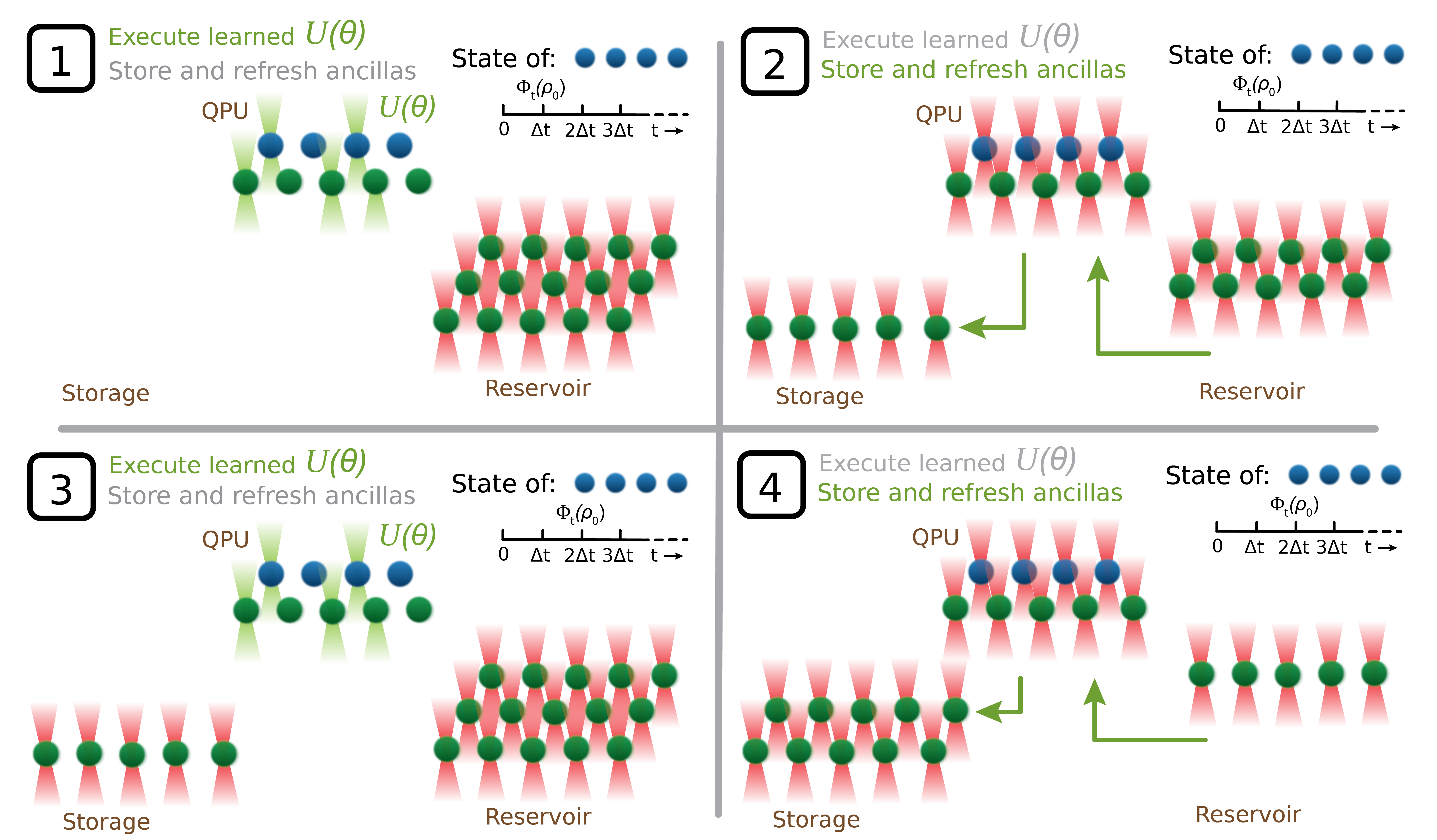
   Figure 3: A neutral atom implementation of a two time step, four qubit quantum channel approximation using five ancilla qubits by iteratively applying the Stinespring unitary to the computational qubits and a new set of ancilla qubits every iteration. 1) In the quantum processing unit (QPU) the Stinespring unitary is performed to evolve $\rho_{0}$ to $\Phi_{\Delta t}(\rho_{0})$. 2) Using movable tweezers, the entangled ancillas are deposited in the storage and new ancillas are brought in from the reservoir. 3,4) The processes of 1) and 2) are repeated to evolve $\Phi_{\Delta t}(\rho_{0})$ to $\Phi_{2\Delta t}(\rho_{0})$.

   

  

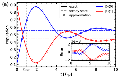
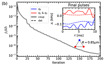
Figure 4: Quantum channel approximations for a target quantum channel describing single qubit decay with $\gamma_{\text{tqc}}=0.5$ and $\Omega_{\text{tqc}}=0.5$, both in units of $1/T_{\text{tqc}}$. The algorithm is trained on 10 randomly sampled initial states combined with all 4 Pauli strings to give $L=40$. Two time steps of training are used, such that we have $t_{\text{train}}=2\Delta t$. Two ancilla qubits are taken, with all qubits positioned in an equilateral triangle. (a) Exact, approximated and steady state populations (with errors) for a single state not in the training data set. (b) Convergence of error $J_{1}(U)$ together with the final pulses on all qubits.

$$d_{\text{Bures}}(\rho,\rho^{\prime})^{2}=2\left(1-\operatorname{Tr}\left[\left(\sqrt{\rho}\rho^{\prime}\sqrt{\rho}\right)^{\frac{1}{2}}\right]\right)\leq 2.$$ (17)

and take the average over the evolution of 10 different initial states, which are not in the training set. The arbitrary timescale of the target quantum channel (tqc) is $T_{\text{tqc}}$ and is independent of the state preparation timescale $\tau_{f}$.

In the results in this section, we will train on all Pauli strings. Thus, every initial state $\rho_{0,l}$ is measured against every Pauli string. Furthermore, we will always use Van der Waals (VdW) interactions between the qubits with $R=0.85\,\mu$m between nearest neighbor qubits and $C_{6}=0.037\,$kHz/$\mu$m⁶ such that $V=0.1\,$kHz between nearest neighbors (cf. Appendix B). For all considered target quantum channels except the 1 qubit case, no analytic solution is known. Thus, we approximate the exact solution by a high-accuracy numerical solver for the error analysis. The pulses are discretized as equidistant step functions with $N=100$ steps.

1 Qubit decay

The evolution of a single qubit decaying from $|1\rangle$ to $|0\rangle$ with rate $\gamma_{\text{tqc}}$ and undergoing Rabi oscillations with frequency $\Omega_{\text{tqc}}$ is given by the Lindbladian, as in Eq. (1), with

$$H=\frac{\Omega}{2}\begin{pmatrix}0&1\\ 1&0\end{pmatrix},\,\,A_{0}=\begin{pmatrix}0&1\\ 0&0\end{pmatrix},\,\,\rho(0)=\begin{pmatrix}\rho_{00}&\rho_{01}\\ \overline{\rho_{01}}&1-\rho_{00}\end{pmatrix}.$$

The dynamics of this system allow for the state to be described analytically (cf. App. C), allowing for exact calculations of the errors of the quantum channel approximation.

By the Stinespring dilation theorem (cf. Sec. II), at most two ancilla qubits are necessary to approximate this target quantum channel. We want to approximate single qubit decay with $\gamma_{\text{tqc}}=\Omega_{\text{tqc}}=0.5$, in units of $1/T_{\text{tqc}}$. From Fig. 4, we see that after minimizing the loss function (cf. Eq. (8)), the quantum channel approximation becomes extremely accurate. Furthermore, the pulses retrieved are smooth and implementable on an actual quantum computing system. Note that because of spatial symmetry between the two ancilla qubits and the computational qubit, the optimal pulses on the ancilla qubits are equal. The Bures error averaged over 10 new initial states on the first time step is $8.3\cdot 10^{-7}$ and rises up to $5.1\cdot 10^{-6}$ after 9 reapplications of the unitary circuit. From the figure and the evolution of the average Bures error, we see that the behavior of the quantum channel can be accurately predicted for longer times without the error increasing significantly. This is especially interesting as no knowledge on the system after $t_{\text{train}}$ is assumed.

2 Qubit decay

As a more complicated case, we consider a quantum channel describing two decaying, and interacting qubits. By the Stinespring dilation theorem (cf. Sec. II), we know that we need a maximum of four ancilla qubits. However, as we only have two decay terms, we only need two additional ancilla qubits. Nevertheless, to open up the search space, we choose to implement three ancilla qubits. For the target quantum channel, we take $\gamma_{1,\text{tqc}}=0.5,$ $\Omega_{1,\text{tqc}}=0.3,$ $\gamma_{2,\text{tqc}}=0.3,$ $\Omega_{2,\text{tqc}}=0.2$, all in units of $1/T_{\text{tqc}}$, to ensure that there is no symmetry between the qubits. Furthermore, their interaction strength is $V_{\text{tqc}}=0.1\,[1/T_{\text{tqc}}]$. All of this leads to non-trivial behavior over the populations (see solid lines in Fig. 5a).

   

  

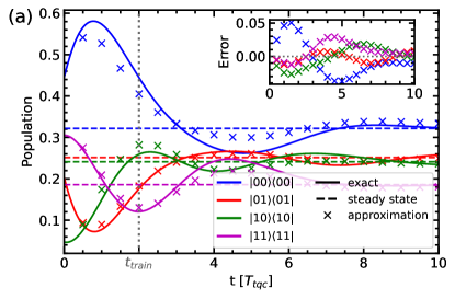
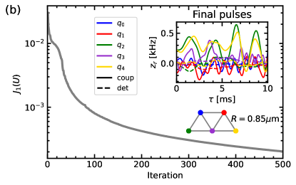
Figure 5: Quantum channel approximations for a quantum channel describing two decaying qubits with interaction. The parameters of the target quantum channel are $\gamma_{1,tqc}=0.5$ and $\Omega_{1,tqc}=0.3$ for qubit 1, $\gamma_{2,tqc}=0.3$ and $\Omega_{2,tqc}=0.2$ for qubit 2 and an interaction strength of $V_{tqc}=0.1$, all in units of $1/T_{\text{tqc}}$. The algorithm is trained on 20 randomly sampled initial states combined with all 16 Pauli strings to give $L=320$. Three ancilla qubits are taken so that all qubits are positioned as two equilateral triangles in an “M” shape. (a) Exact, approximated and steady state populations (with errors) for a single state not included in the training data. (b) Convergence of error $J_{1}(U)$ together with the final pulses on all qubits.

From Fig. 5, we see that learning the target quantum channel becomes harder as the Pauli trace errors remains larger than in the single qubit results of Sec. V. One can clearly see this in the population figure, as the populations are no longer precisely predicted. Furthermore, the average Bures error on the first time step is $9.0\cdot 10^{-4}$, which is significantly higher than for the single qubit target quantum channel. Despite this, it is remarkable to see that the qualitative behavior of the evolution is well predicted, even far beyond the training time $t_{\text{train}}$.

Transverse Field Ising model

We analyze the transverse field Ising model (TFIM) with decay as a use case of our method outside quantum computing Stinchcombe (1973). In this model, spins interact with a transverse magnetic field as well as with their nearest neighbors. For spins aligned in a straight line, the TFIM Hamiltonian takes the form

$$H=-B_{\text{tqc}}\sum_{i}X_{i}+J_{\text{tqc}}\sum_{i}Z_{i}Z_{i+1},$$ (18)

with $Z_{i}$ and $X_{i}$ respectively the Pauli $Z$-operator and Pauli $X$-operator on qubit $i$, $J_{\text{tqc}}$ the coupling strength and $B_{\text{tqc}}$ the transverse external field strength, both in units of $1/T_{\text{tqc}}$. Fig. 6 shows results for a 2 spin TFIM. The average Bures error on the first time step is $2.3\cdot 10^{-3}$. Similar to the 2 qubit case of Fig. 5, we see increasing errors for higher extrapolation times, but good prediction of the general behavioral trend of the evolution. This shows that the algorithm can properly handle target quantum channels which are not related to the system they are approximated on.

   

  

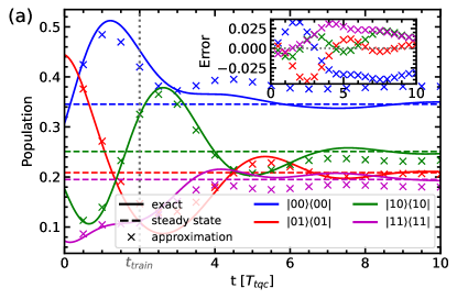
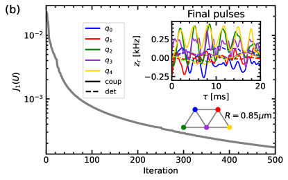
Figure 6: Quantum channel approximations for a 2 qubit TFIM model with $B_{\text{tqc}}=0.5$, $J_{\text{tqc}}=0.4$, $\gamma_{0,\text{tqc}}=0.5$, and $\gamma_{1,\text{tqc}}=0.3$, in units of $1/T_{\text{tqc}}$. For the approximating qubit system, we take the same parameters and training setup as in Fig. 5. (a) Exact, approximated and steady state populations (with errors) for a single state not included in the training data set. (b) Convergence of error $J_{1}(U)$ together with the final pulses on all qubits.

.

.

Pulse-based vs. gate-based

In the current NISQ-era, gate-based optimization methods are most widely implemented. In recent works, it has been suggested that stochastic and pulse-based methods can lead to higher expressibility and faster convergence of the optimization Magann et al. (2021); de Keijzer et al. (2023a); Harwood et al. (2022); Sweke et al. (2020). For our algorithm, we compare gate-, stochastic gate-, and pulse-based methods using the notion of equivalent evolution processes de Keijzer et al. (2023a), which considers that for all methods, the system evolves under the most similar circumstances. Concretely, this means all methods are run on a quantum computation system with similar controls, entanglement operations and evolution times.

We consider control over the coupling strength $\Omega$ for the pulse-based method, and a hardware efficient ansatz with $ZXZ$ parametrized gates for the gate-based method, both resulting in full rotational control of the Bloch sphere de Keijzer et al. (2023a). Furthermore, we consider a VdW drift Hamiltonian $H_{d}$ and entanglement gates $U_{ent}=\exp(-iH_{d}\tau_{V})$ for the gate-based method. We assume $V=0.07$ kHz with $R=0.9\mu$m and $C_{6}=0.037$ kHz$/\mu$m⁶. In order to supply enough time for entanglement, we take $\tau_{V}=1/V=10$ ms and take Rabi frequencies in the order of 1 kHz to get $\tau_{g}=1$ ms. To get similar evolutions, we take $\tau_{f,\text{pulse}}=\tau_{f,\text{gate}}$, which completes the construction of the equivalent evolution processes. To add stochasticity to the gate-based optimization, we uniformly select a random subset of gates to update the parameters for each iteration instead of optimizing the entire gate set.

In Fig. 7 we compare the average Bures distances over time for the unitary approximations based on a gate based, a stochastic gate based and a pulse based method, each trained for the same number of $\#\text{QE}$. The target quantum channel is again a decay model on two qubits with $\gamma_{1,tqc}=0.3$ and $\Omega_{1,tqc}=0.5$ for qubit 1, $\gamma_{2,tqc}=0.2$ and $\Omega_{2,tqc}=0.35$ for qubit 2 and an interaction strength of $V_{tqc}=0.2$, all in units of $1/T_{\text{tqc}}$. The pulse based method and the stochastic gate based method perform very similar, while both outperform the gate based method. We hypothesize that the pulse based method can be improved by adding stochasticity as well. Note that this comparison was done on a data set where all three methods went through a gradient descent. In our simulations, we find that for many training data sets, the gate based methods had problems with finding good local minima of the loss function.

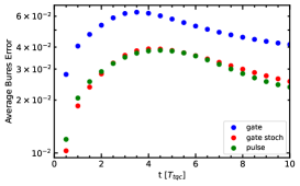
Figure 7: Comparison of the evolution over time of the Bures error for a gate-based, a stochastic gate-based, and a pulse-based approach. The target quantum channel is a decay model on two qubits with $\gamma_{1,tqc}=0.3$ and $\Omega_{1,tqc}=0.5$ for qubit 1, $\gamma_{2,tqc}=0.2$ and $\Omega_{2,tqc}=0.35$ for qubit 2 and an interaction strength of $V_{tqc}=0.2$, all in units of $1/T_{\text{tqc}}$. The Bures error is the average of the predictions on 10 new states. Training done using the notion of equivalent evolutions and for the same number of quantum evaluations $\#\text{QE}$.

VI Conclusion

In this work, we introduce an algorithm for quantum channel approximation and extrapolation. This method differentiates itself from previous work by being able to approximate the quantum channel based purely on measurement data, and the inclusion of multiple time steps plus steady state behavior. The method variationally learns the Stinespring unitary describing the quantum channel at a fixed time $\Delta t$, either through a gate- or pulse-based method. This approximation can later be extrapolated to make future time predictions for the quantum channel behavior at discrete multiples of $\Delta t$. The method has, through simulations, shown proof of concept for non-trivial target quantum channels based on NISQ qubits and Ising models. An analysis between gate- and pulse-based implementations of the algorithm, using equivalent evolution processes, has shown that adding stochasticity or switching to a pulse-based method is beneficial for approximating quantum channels given small state preparation times, which is especially important for mitigating decoherence in the NISQ era.

Furthermore, it is reasoned that a neutral atom quantum computing system is very well-suited for executing this algorithm. The algorithm requires numerous ancilla qubits that need to be coherently moved and stored without being controlled, which neutral atom systems are adapted for given their high scalability, long coherence times, and modifiable qubit topologies.

In future work, it would be of interest to split the approximation of the quantum channel into a part that is unitary on the computational qubits and a part that is a dilation, as in Jong et al. (2021). By separating these two contributions, the model could potentially become less complex and better suited for cases where the unitary evolution and decoherence act on different timescales. Another direction of improvement would be in using prior information on the quantum channel to improve convergence. We hypothesize that by knowing the Kraus decomposition Brasil et al. (2013) or steady state, it could be possible to construct a set of observables and initial states that provides more information on the channel’s behavior.

Data Availability

The data that support the findings of this study are available from the corresponding author upon reasonable request.

Appendix A Multiple time step methods

A possibility of improving the learning capabilities of our method is training with data on multiple time steps. If measurements on $\Phi_{n\Delta t}(\rho_{0})$ for $n\in[1,2,\cdots,N]$ are known, the loss function can be redefined as

$$J_{1}(U)=\sum_{n=1}^{N}\sum_{l=1}^{L}\operatorname{Tr}_{A}[O_{l}(\rho^{\prime}_{l,n}-\rho_{l,n})]^{2},$$ (19)

with

$$\rho_{l,n}=\Phi_{n\Delta t}(\rho_{l,0})=\underbrace{\Phi_{\Delta t}(\Phi_{\Delta t}(\cdots\Phi_{\Delta t}(\rho_{l,0})\cdots))}_{n\text{ repeated applications}}\text{, and }\rho^{\prime}_{l,n}=\operatorname{Tr}_{B}[U\cdot\rho^{\prime}_{l,n-1}\otimes|0\rangle\langle 0|_{B}\cdot U^{\dagger}],\qquad\rho^{\prime}_{l,0}=\rho_{l,0}.$$ (20)

Straightforward variational differentiation in the pulse-based case shows that the Fréchet derivative $\frac{\delta}{\delta U}J_{1}$ for two time steps ($n=2$) is given by

$$\frac{\delta}{\delta U}J_{1} =4\delta(\tau_{f}-\tau)\sum_{l=1}^{L}\Big{(}\operatorname{Tr}_{A}[O_{l}(\rho^{\prime}_{l,1}-\rho_{l,1})]\times\left(O_{l}\otimes I_{B}\cdot U\cdot\rho^{\prime}_{l,0}\otimes|0\rangle\langle 0|_{B}\right)$$ (21)

$$+\operatorname{Tr}_{A}[O_{l}(\rho^{\prime}_{l,2}-\rho_{l,2})]\times\left(O_{l}\otimes I_{B}\cdot U\cdot\rho^{\prime}_{l,1}\otimes|0\rangle\langle 0|_{B}\right)$$

$$+\operatorname{Tr}_{A}[O_{l}(\rho^{\prime}_{l,2}-\rho_{l,2})]\times\operatorname{Tr}_{B}[U^{\dagger}\cdot O_{l}\otimes I_{B}\cdot U\cdot I_{A}\otimes|0\rangle\langle 0|_{B}]\otimes I_{B}\cdot U\cdot\rho^{\prime}_{l,0}\otimes|0\rangle\langle 0|_{B}\Big{)}.$$

This can be extended to show that the Fréchet derivative $\frac{\delta}{\delta U}J_{1}$ for $n$ time steps is given by

$$\frac{\delta}{\delta U}J_{1}=4\delta(\tau_{f}-\tau)\sum_{n=1}^{N}\sum_{l=1}^{L}\sum_{k=0}^{n-1}\operatorname{Tr}_{A}[O_{l}(\rho^{\prime}_{l,n}-\rho_{l,n})]\times\left(O_{l,k}\otimes I_{B}\cdot U\cdot\rho^{\prime}_{l,n-k-1}\otimes|0\rangle\langle 0|_{B}\right),$$ (22)

with $O_{l,k}$ defined as

$$O_{l,k}=\operatorname{Tr}_{B}[U^{\dagger}\cdot O_{l,k-1}\otimes I_{B}\cdot U\cdot I_{A}\otimes|0\rangle\langle 0|_{B}],\qquad O_{l,0}=O_{l}.$$ (23)

This gradient is very similar to the one in Eq. (14). However, finding a way to measure $O_{l,k}$ as observable is not directly possible. Instead, $O_{l,0}$ has to be measured w.r.t. the entire entangled system, including all previously entangled sets of ancillas. The number of quantum state evaluations to calculate the gradient for multiple time steps is increased by a factor $\frac{1}{2}N(N-1)$ over the single time step method, for a total of $\#\text{QE}=\frac{1}{2}N(N-1)KLR$ quantum state evaluations per gradient calculation.

Appendix B Rydberg Physics

This section introduces basic Rydberg physics to identify what drift and control Hamiltonians as in Eq. (11) can look like on a Rydberg atom quantum computing system. This also yields candidates for the control operators $Q_{r}$, as in Eq. (12). For this section, we assume gr qubits Saffman (2016b) such that the $|1\rangle$ state is a Rydberg state.

The Rydberg states have a passive ‘always-on’ interaction, which is described by a drift Hamiltonian $H_{d}$, depending on the choice of qubits scheme Morgado and Whitlock (2021), as a Van der Waals interaction (VdW) Shi and Lu (2021) or a dipole-dipole interaction (dip) Young et al. (2021)

$$H_{d,\text{VdW}} =\sum_{i=1}^{m}\sum_{j=1}^{m}\frac{C_{6}}{R_{ij}^{6}}|11\rangle_{ij}\langle 11|_{ij},$$ (24)

$$H_{d,\text{dip}} =\sum_{i=1}^{m}\sum_{j=1}^{m}\frac{C_{3}}{R_{ij}^{3}}\left(|01\rangle_{ij}\langle 10|_{ij}+\text{h.c.}\right),$$

where $R_{ij}$ is the interatomic distance. We also define the characteristic interaction as $V:=C_{n}/\min_{ij}{(R_{ij}^{n})},\,n\in\{3,6\}.$

To perform single qubit manipulations on qubit $j$, a laser interacts with the atom to realize the Hamiltonian Morgado and Whitlock (2021); Saffman (2016a); Adams et al. (2019)

$$H_{j}^{01}(\tau)=\frac{\Omega_{j}(\tau)}{2}\left(e^{i\varphi_{j}(\tau)}|0\rangle_{j}\langle 1|_{j}+e^{-i\varphi_{j}(\tau)}|1\rangle_{j}\langle 0|_{j}\right)-\Delta_{j}(\tau)|1\rangle_{j}\langle 1|_{j}.$$ (25)

Here, $\Omega_{j}(\tau)$ denotes the coupling strength, $\varphi_{j}(\tau)$ the phase of the laser coupled to atom $j$, and $\Delta_{j}(\tau)$ = $\omega_{j}(\tau)-\omega_{0}$ the detuning of the laser frequency $\omega_{j}(\tau)$ from the energy level difference $\omega_{0}$.

The control Hamiltonian $H_{c}$ can contain several terms depending on which of the mentioned laser parameters can be controlled. In general, the control Hamiltonian takes the form

$$H_{c}[z(\tau)]=\sum_{r=1}^{R}Q_{r}z_{r}(\tau)+Q_{r}^{\dagger}\overline{z_{r}(\tau)},$$ (26)

where $z_{r}(\tau)\in\mathbb{C}$, and $Q_{r}$ is a $m$-qubit operator. The choice of $z_{r}(\tau)$ being a complex number stems from the fact that it could represent both the coupling strength and the phase in Eq. (25). In this work, we assume no control over the phase such that in all cases $z_{r}(\tau)\in\mathbb{R}$. For the control Hamiltonian $H_{c}$

$$H_{c}[z]=H_{c}^{\text{coup}}[z^{\text{coup}}]+H_{c}^{\text{det}}[z^{\text{det}}],$$

with $z=(z^{\text{coup}},z^{\text{det}}),$ $R=2m$. Here, the coupling control $H_{c}^{\text{coup}}$ and detuning control $H_{c}^{\text{det}}$ take the form of Eq. (26) with

$$Q_{r}^{\text{coup}}=|0\rangle\langle 1|_{r}\quad\text{and}\quad Q_{r}^{\text{det}}=|1\rangle\langle 1|_{r},$$

respectively. Notice that having both coupling and detuning allows for full control on the Bloch sphere of each individual qubit. This is why this term is also referred to as rotational control Lee et al. (2017).

Appendix C Single qubit decay

A single qubit decaying from $|1\rangle$ to $|0\rangle$ with rate $\gamma$ and undergoing Rabi oscillations with frequency $\Omega$ is described by the Lindblad equation, with

$$H=\frac{\Omega}{2}\begin{pmatrix}0&1\\ 1&0\end{pmatrix},\qquad A=\begin{pmatrix}0&1\\ 0&0\end{pmatrix},\qquad\rho(0)=\begin{pmatrix}\rho_{00}&\rho_{01}\\ \overline{\rho_{01}}&1-\rho_{00}\end{pmatrix}.$$

The dynamics of this system allow for the state to be described analytically as

$$\rho_{00}(t) =B+(\rho_{00}-B)\exp\left(-\frac{3}{4}\gamma t\right)\left(\cosh\left(\frac{1}{4}tF\right)+\frac{C}{F}\sinh\left(\frac{1}{4}tF\right)\right),$$ (27)

$$\rho_{01}(t) =B^{\prime}+\operatorname{Re}\left(\rho_{01}\right)\exp\left(-\frac{1}{2}\gamma t\right)+\left(i\operatorname{Im}\left(\rho_{01}\right)-B^{\prime}\right)\exp\left(-\frac{3}{4}\gamma t\right)\left(\cosh\left(\frac{1}{4}tF\right)+\frac{C^{\prime}}{F}\sinh\left(\frac{1}{4}tF\right)\right),$$

with $F=\sqrt{\gamma^{2}-16\Omega^{2}}$ and

$$B=\frac{\gamma^{2}+\Omega^{2}}{\gamma^{2}+2\Omega^{2}} ,\qquad C=-\gamma-\gamma\frac{4\Omega^{2}}{(1-\rho_{00})\gamma^{2}+(1-2\rho_{00})\Omega^{2}},$$ (28)

$$B^{\prime}=\frac{i\gamma\Omega}{\gamma^{2}+2\Omega^{2}} ,\qquad C^{\prime}=\gamma-4\Omega\frac{(1-\rho_{00})\gamma^{2}+(1-2\rho_{00})\Omega^{2}}{\operatorname{Im}\left(\rho_{01}\right)(\gamma^{2}+2\Omega^{2})-\gamma\Omega}.$$

References

- Preskill (2018) J. Preskill, Quantum 2, 79 (2018).
- Arute et al. (2019) F. Arute, K. Arya, R. Babbush, D. Bacon, J. C. Bardin, et al., Nature 574, 505 (2019).
- Kandala et al. (2017) A. Kandala, A. Mezzacapo, K. Temme, M. Takita, M. Brink, J. M. Chow, and J. M. Gambetta, Nature (London) 549, 242 (2017), arXiv:1704.05018 [quant-ph] .
- Hempel et al. (2018) C. Hempel, C. Maier, J. Romero, J. McClean, T. Monz, H. Shen, P. Jurcevic, B. P. Lanyon, P. Love, R. Babbush, A. Aspuru-Guzik, R. Blatt, and C. F. Roos, Phys. Rev. X 8, 031022 (2018).
- Aspuru-Guzik and Walther (2012) A. Aspuru-Guzik and P. Walther, Nature Physics 8 (2012), 10.1038/nphys2253.
- O’Brien et al. (2018) T. E. O’Brien, P. Rożek, and A. R. Akhmerov, Phys. Rev. Lett. 120, 220504 (2018).
- Arute et al. (2020) F. Arute, K. Arya, R. Babbush, D. Bacon, J. C. Bardin, R. Barends, et al., Science 369, 1084 (2020).
- Del Re et al. (2020) L. Del Re, B. Rost, A. F. Kemper, and J. K. Freericks, Phys. Rev. B 102, 125112 (2020).
- Jong et al. (2021) W. Jong, M. Metcalf, J. Mulligan, M. Płoskoń, F. Ringer, and X. Yao, Physical Review D 104 (2021), 10.1103/PhysRevD.104.L051501.
- Wang et al. (2023) Y. Wang, E. Mulvihill, Z. Hu, N. Lyu, S. Shivpuje, Y. Liu, M. B. Soley, E. Geva, V. S. Batista, and S. Kais, Journal of Chemical Theory and Computation (2023), 10.1021/acs.jctc.3c00316.
- Brasil et al. (2013) C. A. Brasil, F. F. Fanchini, and R. d. J. Napolitano, Revista Brasileira de Ensino de Física 35, 01 (2013).
- Foss-Feig et al. (2021) M. Foss-Feig, D. Hayes, J. M. Dreiling, C. Figgatt, J. P. Gaebler, S. A. Moses, J. M. Pino, and A. C. Potter, Phys. Rev. Res. 3, 033002 (2021).
- Bluvstein et al. (2022) D. Bluvstein, H. Levine, G. Semeghini, T. T. Wang, S. Ebadi, M. Kalinowski, A. Keesling, N. Maskara, H. Pichler, M. Greiner, V. Vuletić, and M. D. Lukin, Nature 604, 451 (2022).
- Schlimgen et al. (2022) A. W. Schlimgen, K. Head-Marsden, L. M. Sager, P. Narang, and D. A. Mazziotti, Phys. Rev. Res. 4, 023216 (2022).
- Hu et al. (2020) Z. Hu, R. Xia, and S. Kais, Scientific Reports 10 (2020), 10.1038/s41598-020-60321-x.
- Head-Marsden et al. (2021) K. Head-Marsden, S. Krastanov, D. A. Mazziotti, and P. Narang, Phys. Rev. Res. 3, 013182 (2021).
- Hu et al. (2022) Z. Hu, K. Head-Marsden, D. A. Mazziotti, P. Narang, and S. Kais, Quantum 6, 726 (2022).
- Patsch et al. (2020) S. Patsch, S. Maniscalco, and C. P. Koch, Phys. Rev. Res. 2, 023133 (2020).
- Schlimgen et al. (2021) A. W. Schlimgen, K. Head-Marsden, L. M. Sager, P. Narang, and D. A. Mazziotti, Phys. Rev. Lett. 127, 270503 (2021).
- McArdle et al. (2019) S. McArdle, T. Jones, S. Endo, Y. Li, S. C. Benjamin, and X. Yuan, npj Quantum Information 5, 75 (2019).
- Hornberger (2009) K. Hornberger, Entanglement and Decoherence: Foundations and Modern Trends , 221 (2009).
- Weinberg (2016) S. Weinberg, Physical Review A 94, 042117 (2016).
- Holevo (2019) A. S. Holevo, Quantum Systems, Channels, Information, A Mathematical Introduction (De Gruyter, Berlin, Boston, 2019).
- Shalit (2020) O. Shalit, “Dilation theory: a guided tour,” (2020), arXiv:2002.05596 [math.OA] .
- Keyl (2002) M. Keyl, Physics Reports 369, 431 (2002).
- Gogolin et al. (2021) C. Gogolin, G.-L. Anselmetti, D. Wierichs, and R. M. Parrish, New Journal of Physics (2021).
- Saffman (2016a) M. Saffman, Journal of Physics B: Atomic, Molecular and Optical Physics 49, 202001 (2016a).
- de Keijzer et al. (2022) R. de Keijzer, V. Colussi, B. Škorić, and S. Kokkelmans, AVS Quantum Science 4, 013803 (2022), https://pubs.aip.org/avs/aqs/article-pdf/doi/10.1116/5.0076435/16493383/013803_1_online.pdf .
- Schuld et al. (2019) M. Schuld, V. Bergholm, C. Gogolin, J. Izaac, and N. Killoran, Phys. Rev. A 99, 032331 (2019).
- Asthana et al. (2022) A. Asthana, C. Liu, O. R. Meitei, S. E. Economou, E. Barnes, and N. J. Mayhall, arXiv (2022), 10.48550/ARXIV.2203.06818.
- Meitei et al. (2021) O. R. Meitei, B. T. Gard, G. S. Barron, D. P. Pappas, S. E. Economou, E. Barnes, and N. J. Mayhall, npj Quantum Information 7, 155 (2021).
- Magann et al. (2021) A. B. Magann, C. Arenz, M. D. Grace, T.-S. Ho, R. L. Kosut, J. R. McClean, H. A. Rabitz, and M. Sarovar, PRX Quantum 2, 010101 (2021).
- de Keijzer et al. (2023a) R. de Keijzer, O. Tse, and S. Kokkelmans, Quantum 7, 908 (2023a).
- Butenko and Pardalos (2015) S. Butenko and P. M. Pardalos, Numerical Methods and Optimization: An introduction (CRC Press, 2015).
- Ma et al. (2022) S. Ma, A. P. Burgers, G. Liu, J. Wilson, B. Zhang, and J. D. Thompson, Phys. Rev. X 12, 021028 (2022).
- Evered et al. (2023) S. J. Evered, D. Bluvstein, M. Kalinowski, S. Ebadi, T. Manovitz, H. Zhou, S. H. Li, A. A. Geim, T. T. Wang, N. Maskara, H. Levine, G. Semeghini, M. Greiner, V. Vuletic, and M. D. Lukin, “High-fidelity parallel entangling gates on a neutral atom quantum computer,” (2023), arXiv:2304.05420 [quant-ph] .
- Madjarov (2021) I. Madjarov, Entangling, Controlling, and Detecting Individual Strontium Atoms in Optical Tweezer Arrays, Ph.D. thesis, Caltech (2021).
- Weiss and Saffman (2017) D. S. Weiss and M. Saffman, Physics Today 70, 44 (2017), https://doi.org/10.1063/PT.3.3626 .
- de Keijzer et al. (2023b) R. de Keijzer, O. Tse, and S. Kokkelmans, Phys. Rev. A 108, 023122 (2023b).
- Saffman (2016b) M. Saffman, Journal of Physics B: Atomic, Molecular and Optical Physics 49, 202001 (2016b).
- Wu et al. (2021) X. Wu, X. Liang, Y. Tian, F. Yang, C. Chen, Y.-C. Liu, M. K. Tey, and L. You, Chinese Physics B 30, 020305 (2021).
- Young et al. (2020) A. W. Young, W. J. Eckner, W. R. Milner, D. Kedar, M. A. Norcia, E. Oelker, N. Schine, J. Ye, and A. M. Kaufman, Nature 588, 408 (2020).
- Stinchcombe (1973) R. B. Stinchcombe, Journal of Physics C: Solid State Physics 6, 2459 (1973).
- Harwood et al. (2022) S. M. Harwood, D. Trenev, S. T. Stober, P. Barkoutsos, T. P. Gujarati, S. Mostame, and D. Greenberg, ACM Transactions on Quantum Computing 3 (2022), 10.1145/3479197.
- Sweke et al. (2020) R. Sweke, F. Wilde, J. Meyer, M. Schuld, P. K. Faehrmann, B. Meynard-Piganeau, and J. Eisert, Quantum 4, 314 (2020).
- Morgado and Whitlock (2021) M. Morgado and S. Whitlock, AVS Quantum Science 3, 023501 (2021), https://doi.org/10.1116/5.0036562 .
- Shi and Lu (2021) X.-F. Shi and Y. Lu, Phys. Rev. A 104, 012615 (2021).
- Young et al. (2021) J. T. Young, P. Bienias, R. Belyansky, A. M. Kaufman, and A. V. Gorshkov, Physical Review Letters 127 (2021), 10.1103/physrevlett.127.120501.
- Adams et al. (2019) C. S. Adams, J. D. Pritchard, and J. P. Shaffer, Journal of Physics B: Atomic, Molecular and Optical Physics 53, 012002 (2019).
- Lee et al. (2017) H.-g. Lee, Y. Song, and J. Ahn, Phys. Rev. A 96, 012326 (2017).