Constraints on the speed of sound in the k-essence model of dark energy

Abstract

We consider a particular k-essence scalar field model for the late-time cosmic acceleration in which the sound speed, parametrized as $c_{s}$ is constant. We compute the relevant background and perturbation quantities corresponding to the observables like cosmic microwave background, type Ia supernova, cosmic chronometers, baryon acoustic oscillations, and the $f\sigma_{8}$. We put constraints on the $c_{s}^{2}$ parameter from these observations along with other parameters. We find lower values of $c_{s}^{2}$ which are close to zero are tightly constrained. Particularly, we find mean value of $\log_{\rm 10}(c_{s}^{2})$ to be $-0.61$ and $c_{s}^{2}\leq 10^{-3}$ is more than 3$\sigma$ away from this mean value. This means these observations favor a homogeneous dark energy component compared to the clustering one.

1 Introduction

The late time cosmic acceleration is confirmed by the several cosmological observations like the type Ia supernova observations [1, 2, 3, 4, 5, 6, 7, 8], cosmic microwave background (CMB) observations [9, 10, 11], and the baryon acoustic oscillation observations [12, 13, 14]. Ever since the discovery of the late time cosmic acceleration, an enormous amount of effort has been given to model this phenomenon. The two broad categories of this effort are the notion of the existence of an exotic matter called the dark energy [15, 16, 17, 18, 19, 20] and the modification of gravity[21, 22, 23, 24, 25, 26, 27, 28, 29]. In the first case, the dark energy is assumed to have large negative pressure which causes the late time cosmic acceleration.

There are several dark energy models in the literature [18]. The most simple dark energy model is the $\Lambda$CDM model, in which the cosmological constant $\Lambda$ is the candidate for the dark energy whose energy density is considered to be a constant [30]. This is the most successful model till now which can explain late-time cosmic acceleration. However, this model has some shortcomings, both from theoretical background like the cosmic coincidence and fine-tuning problems [31, 32, 33, 34] and the observations point of view like corresponding to the Hubble tension[35, 36, 37, 38] and the $\sigma_{8}$ tension [39, 40, 41, 42]. It is thus important to study the cosmic acceleration with the models beyond the $\Lambda$CDM.

Different dark energy models affect cosmological evolution differently. If we assume the dark energy is homogeneous, it only affects the cosmological evolution through the background expansion and it does not participate in the clustering. This is the case for the $\Lambda$CDM model. However, there is no a priori reason to consider dark energy to be homogeneous. On the other hand, the inhomogeneous dark energy participates in the clustering. Hence the evolution of perturbations is different in inhomogeneous dark energy compared to the homogeneous one [43]. Thus, it is required to check whether a dark energy is homogeneous or not.

For this purpose, we consider one popular class of dark energy models, named the k-essence [44, 45, 46, 47, 48, 49, 50, 51, 52, 53, 54]. In k-essence model, the late time acceleration is caused by a generic scalar field whose kinetic term can be both canonical and non-canonical. The canonical kinetic term corresponding to a subclass called quintessence [55, 56, 57, 58, 59, 60]. In the quintessence model of dark energy, the speed of sound is unity. For this case, the perturbation in the scalar field is negligible. Consequently, this corresponds to the homogeneity of the dark energy. In the non-canonical k-essence scenario, the sound speed of dark energy is different from unity and it can have values lower than $1$. If the sound speed of dark energy decreases from $1$, the inhomogeneities in the dark energy may increase. For a nice review, see [43] (also see [61, 62, 63]).

In general, any non-canonical k-essence model has an evolving speed of sound. One has to choose a model in such a way that the sound speed is always subluminal because we do not expect any information to propagate faster than the speed of light in a vacuum. Also, the sound speed has to be real. One of the easy ways to maintain such conditions is to choose a non-canonical kinetic term such that the sound speed is constant and can be parameterized. The non-canonical k-essence model with constant sound speed has been studied in the literature like in [64, 65, 66].

In [64], authors have used Planck-2013 results on CMB anisotropy and other cosmological data to put constraints on the speed of sound and found no preferences of a particular value of it in the range between $0$ to $1$. In [65], authors did a similar kind of analysis but with more recent data sets and found similar kinds of results. A few similar kinds of analyses have been done in the literature but with different dark energy models [67, 68, 69]. In this study, we consider such a k-essence model in which the speed of sound is constant during the entire cosmological evolution. With this model, we study the effect of the sound speed of dark energy both in the background and the perturbation evolutions and put constraints on the sound speed of dark energy from the recent cosmological data.

Throughout our study, we consider the signature of the metric to be ($+,-,-,-$) and we quote all the expressions in the natural units. This paper is organized as follows. In Sec. 2, we show the derivation of the form of the Lagrangian for which the speed of sound is constant over cosmic time in the k-essence scenario. In Sec. 3, we investigate the k-essence field evolution and the relevant background quantities. In Sec. 4, we find the evolution of the perturbations with the full relativistic perturbation method. In Sec. 5, we rewrite all the relevant background and perturbation equations in a single autonomous system of differential equations. In Sec. 6, we consider the sub-Hubble limit for the evolution equation for the matter overdensity contrast and compare the result with the full relativistic result. In Sec. 7, we briefly mention some observational data, we consider in our analysis. In Sec. 8, we discuss the results of this study. Finally, in Sec. 9, we present a conclusion.

2 K-essence Lagrangian with constant speed of sound

The Lagrangian for a general k-essence scalar field, $\phi$ is given as [70, 71, 72]

$$\mathcal{L}_{K}=\mathcal{L}_{K}(\phi,X),$$ (2.1)

where $X=\frac{1}{2}(\nabla_{\mu}\phi)(\nabla^{\mu}\phi)=\frac{1}{2}(\partial_{\mu}\phi)(\partial^{\mu}\phi)$. The pressure ($P_{\phi}$), the energy density ($\rho_{\phi}$) and the sound speed ($c_{s}^{2}$) for the k-essence scalar field are given as [46, 70, 71, 72]

$$P_{\phi} = \mathcal{L}_{K},$$ (2.2)

$$\rho_{\phi} = 2X\frac{\partial\mathcal{L}_{K}}{\partial X}-\mathcal{L}_{K},$$ (2.3)

$$c_{s}^{2} = \frac{\frac{\partial P_{\phi}}{\partial X}}{\frac{\partial\rho_{\phi}}{\partial X}}=\frac{\frac{\partial\mathcal{L}_{K}}{\partial X}}{2X\frac{\partial^{2}\mathcal{L}_{K}}{\partial X^{2}}+\frac{\partial\mathcal{L}_{K}}{\partial X}},$$ (2.4)

respectively.

We consider a k-essence model in which the speed of sound of the scalar field is constant i.e. $c_{s}^{2}=$ constant. For this case, from Eq. (2.4), we get a differential equation for the Lagrangian given as

$$2X\frac{\partial^{2}\mathcal{L}_{K}}{\partial X^{2}}-\left(\frac{1-c_{s}^{2}}{c_{s}^{2}}\right)\frac{\partial\mathcal{L}_{K}}{\partial X}=0,$$ (2.5)

for $c_{s}^{2}\neq 0$. The general solution for the above differential equation is given as [64, 65, 66]

$$\mathcal{L}_{K}=U(\phi)X^{n}-V(\phi),$$ (2.6)

where $U$ and $V$ are two arbitrary functions of $\phi$; and $n$ is given as

$$n=\frac{1+c_{s}^{2}}{2c_{s}^{2}}=\text{constant}.$$ (2.7)

For the simplicity of the study, we consider a special case where $U(\phi)=1$ and we denote the corresponding Lagrangian as $\mathcal{L}$ given as

$$\mathcal{L}=X^{n}-V(\phi).$$ (2.8)

We stick to this model throughout this study. Eq. (2.7) is alternatively written as

$$c_{s}^{2}=\frac{1}{2n-1}=\text{constant}.$$ (2.9)

As we discussed in the introduction, the speed of sound should satisfy the condition $0<c_{s}^{2}\leq 1$. This corresponds to $n\geq 1$. Note that, the special case of this model, described by the lagrangian in Eq. (2.8), is the quintessence, where $n=1$ and consequently $c_{s}^{2}=1$. For other cases, $c_{s}^{2}$ decreases from the value, $1$ with increasing values of $n$. Here, $V(\phi)$ is a potential term.

In this model, the pressure is the same as the Lagrangian in Eq. (2.8). The energy density is given as

$$\rho_{\phi}=(2n-1)X^{n}+V(\phi).$$ (2.10)

For this model, the energy-momentum tensor, $T^{\mu}_{\nu}$ is given as

$$T^{\mu}_{\nu}=\frac{\partial\mathcal{L}}{\partial(\partial_{\mu}\phi)}(\partial_{\nu}\phi)-\delta^{\mu}_{\nu}\mathcal{L}=nX^{n-1}g^{\mu\sigma}(\partial_{\sigma}\phi)(\partial_{\nu}\phi)-\delta^{\mu}_{\nu}\mathcal{L},$$ (2.11)

where the metric of the space-time is denoted as $g_{\rm\mu\nu}$ and $\delta^{\mu}_{\nu}$ is the usual Kronecker-delta symbol.

The Euler-Lagrangian equation is given as

$$\frac{1}{\sqrt{|g|}}\partial_{\mu}\left[\sqrt{|g|}\frac{\partial\mathcal{L}}{\partial(\partial_{\mu}\phi)}\right]-\frac{\partial\mathcal{L}}{\partial\phi}=0,$$ (2.12)

where $g$ is the determinant of the given metric, $g_{\rm\mu\nu}$. In this model, the above equation consequently becomes

$$\frac{1}{\sqrt{|g|}}\partial_{\mu}\left[\sqrt{|g|}nX^{n-1}g^{\mu\nu}(\partial_{\nu}\phi)\right]+V^{\prime}(\phi)=0.$$ (2.13)

where $V^{\prime}(\phi)=\frac{dV(\phi)}{d\phi}$ and $|g|$ is the modulus of the determinant, $g$.

3 Background cosmology

For the background cosmology, we consider the spatially flat Friedmann-Lemaître-Robertson-Walker (FLRW) metric given as $dS^{2}=dt^{2}-a^{2}(t)dR^{2}$, where $dS^{2}$ is the line element of the space-time, $dR^{2}$ is the 3-dimensional Euclidean space, $t$ is the cosmic time, and $a$ is the cosmic scale factor. In this case, the expression of $X$ is given as $X=\frac{1}{2}\dot{\bar{\phi}}^{2}$, where overhead dot represents the differention w.r.t $t$. Here, we denote the background scalar field as $\bar{\phi}$. Throughout this paper, a quantity with an overhead bar indicates its unperturbed (background) value. So, the background pressure ($\bar{P}_{\phi}$), energy density ($\bar{\rho}_{\phi}$), and equation of state of dark energy ($w_{\phi}$) are given as

$$\bar{P}_{\phi} = \left(\frac{1}{2}\dot{\bar{\phi}}^{2}\right)^{n}-V(\bar{\phi}),$$ (3.1)

$$\bar{\rho}_{\phi} = (2n-1)\left(\frac{1}{2}\dot{\bar{\phi}}^{2}\right)^{n}+V(\bar{\phi}),$$ (3.2)

$$w_{\phi} = \frac{\bar{P}_{\phi}}{\bar{\rho}_{\phi}}=\frac{\left(\frac{1}{2}\dot{\bar{\phi}}^{2}\right)^{n}-V(\bar{\phi})}{(2n-1)\left(\frac{1}{2}\dot{\bar{\phi}}^{2}\right)^{n}+V(\bar{\phi})},$$ (3.3)

respectively.

The background Euler-Lagrangian equation is given as

$$n\left(\frac{1}{2}\dot{\bar{\phi}}^{2}\right)^{n-1}\left[(2n-1)\ddot{\bar{\phi}}+3H\dot{\bar{\phi}}\right]+V^{\prime}(\bar{\phi})=0.$$ (3.4)

The two Friedmann equations are given as

$$3M_{\rm pl}^{2}H^{2} = \bar{\rho}_{\phi}+\bar{\rho}_{m},$$ (3.5)

$$6M_{\rm pl}^{2}(\dot{H}+H^{2}) = -(1+3w_{\phi})\bar{\rho}_{\phi}-\bar{\rho}_{m},$$ (3.6)

where, $\bar{\rho}_{m}$ is the background energy density for the total matter components (including both dark matter and baryons), $H$ is the Hubble parameter, and $M_{\rm pl}^{2}=\frac{1}{8\pi G}$ with $G$ is the Newtonian gravitational constant. Here, we have neglected the radiation, because we are studying the expansion history of the Universe from the matter-dominated era to the present epoch.

3.1 Relevant background quantities

The energy density parameter ($\Omega_{\phi}$) of the scalar field is given as

$$\Omega_{\phi}=\frac{\bar{\rho}_{\phi}}{3M_{\rm pl}^{2}H^{2}}.$$ (3.7)

The matter-energy density parameter, $\Omega_{m}$ is given as

$$\Omega_{m}=1-\Omega_{\phi}.$$ (3.8)

Here, we have neglected the contribution of radiation. The normalized Hubble parameter, $E$ is calculated as

$$E^{2}=\frac{\Omega_{\rm m0}(1+z)^{3}}{\Omega_{m}},$$ (3.9)

where it is defined as $E=\frac{H}{H_{0}}$ with $H_{0}$ being the present value of the Hubble parameter. In the above expression, $\Omega_{\rm m0}$ is the present value of the matter-energy density parameter.

It is also important to calculate the cosmological distances like the luminosity distance. To do this, we define a quantity, $d_{N}$ given as

$$d_{N}=\int_{0}^{z}\frac{d\tilde{z}}{E(\tilde{z})},$$ (3.10)

where $z$ (also $\tilde{z}$) is the cosmological redshift. The luminosity distance, $d_{L}$ and the angular diameter distance, $d_{A}$ is related to $d_{N}$ given as

$$d_{L} = \left(\frac{1}{H_{0}}\right)(1+z)d_{N},$$ (3.11)

$$d_{A} = \left(\frac{1}{H_{0}}\right)\frac{d_{N}}{1+z}.$$ (3.12)

Note that, the above expressions are valid for the spatially flat Universe assumption which we consider throughout our analysis.

4 Evolution of perturbations

Here, we are considering the conformal Newtonian gauge for which the perturbed metric is given as [25, 60]

$$dS^{2}=(1+2\Psi)dt^{2}-a^{2}(1-2\Phi)dR^{2},$$ (4.1)

where $\Phi$ is the gravitational potential. Before proceeding further, we first consider the anisotropic stress to be zero which corresponds to

$$\Psi=\Phi.$$ (4.2)

With the above metric, the first-order Euler-Lagrangian equation becomes

$$2^{1-n}n\left(\dot{\bar{\phi}}^{2}\right)^{n}\left[(2n-1)\ddot{(\delta\phi)}+3H\dot{(\delta\phi)}-2(n+1)\dot{\bar{\phi}}\dot{\Phi}+\frac{k^{2}}{a^{2}}(\delta\phi)\right]$$

$$+2\dot{\bar{\phi}}V^{\prime}(\bar{\phi})\left[(1-n)\dot{(\delta\phi)}+n\dot{\bar{\phi}}\Phi\right]+\dot{\bar{\phi}}^{2}V^{\prime\prime}(\bar{\phi})(\delta\phi)=0,$$ (4.3)

where we have perturbed the scalar field as $\phi=\bar{\phi}+\delta\phi$ and $k$ is the magnitude of wave vector. The above equation is obtained from the Fourier transform of the first-order perturbations. Throughout this study, we mention all the first-order perturbation equations in the Fourier space. The first-order field equations are given as

$$-k^{2}\Phi-3a^{2}H(\dot{\Phi}+H\Phi) = 4\pi Ga^{2}(\delta\rho_{\phi}+\bar{\rho}_{m}\delta_{m}),$$ (4.4)

$$\dot{\Phi}+H\Phi = 4\pi G\left[a(\bar{\rho}_{\phi}+\bar{P}_{\phi})v_{\phi}+a\bar{\rho}_{m}v_{m}\right],$$ (4.5)

$$\ddot{\Phi}+4H\dot{\Phi}+(2\dot{H}+3H^{2})\Phi = 4\pi G(\delta P_{\phi}),$$ (4.6)

where $\bar{\rho}_{m}\delta_{m}$ is the perturbation in the energy density of the matter components, $\bar{\rho}_{m}$ is the background matter energy density and $\delta_{m}$ is the matter overdensity contrast, defined as $\delta_{m}=\frac{\rho_{m}-\bar{\rho}_{m}}{\bar{\rho}_{m}}$, where $\rho_{m}$ is the total matter-energy density. $v_{m}$ is the velocity perturbations in the matter fields. $\delta\rho_{\phi}$, $v_{\phi}$ and $\delta P_{\phi}$ are the first-order perturbations in the energy density, velocity field, and pressure respectively for the scalar field. These are given as

$$\delta\rho_{\phi} = 2^{1-n}n(2n-1)\left(\dot{\bar{\phi}}\right)^{2n-1}\left[\dot{(\delta\phi)}-\dot{\bar{\phi}}\Phi\right]+V^{\prime}(\bar{\phi})\delta\phi,$$ (4.7)

$$a(\bar{\rho}_{\phi}+\bar{P}_{\phi})v_{\phi} = 2^{1-n}n\left(\dot{\bar{\phi}}\right)^{2n-1}\delta\phi,$$ (4.8)

$$\delta P_{\phi} = 2^{1-n}n\left(\dot{\bar{\phi}}\right)^{2n-1}\left[\dot{(\delta\phi)}-\dot{\bar{\phi}}\Phi\right]-V^{\prime}(\bar{\phi})\delta\phi.$$ (4.9)

In general, we need to solve Eqs. (4.3), (4.4), (4.5), and (4.6) simultaneously to find the solutions for $\delta\phi$, $\Phi$, $\delta_{m}$ and $v_{m}$. However, the expressions for these differential equations are such that we do not need to solve all the differential equations simultaneously. Instead, we can only simultaneously solve Eqs. (4.3) and (4.4) to find solutions for $\delta\phi$ and $\Phi$ first, because these two differential equations are in the closed form w.r.t the quantities $\delta\phi$ and $\Phi$ and other two quantities $\delta_{m}$ and $v_{m}$ are not present. Using the solutions of $\delta\phi$ and $\Phi$ in Eqs. (4.5) and (4.6), $\delta_{m}$ and $v_{m}$ can be solved separately. Putting Eq. (4.9) in Eq. (4.5), we get a differential equation for $\Phi$ given as

$$\ddot{\Phi}+4H\dot{\Phi}+(2\dot{H}+3H^{2})\Phi=4\pi G\left(2^{1-n}n\left(\dot{\bar{\phi}}\right)^{2n-1}\left[\dot{(\delta\phi)}-\dot{\bar{\phi}}\Phi\right]-V^{\prime}(\bar{\phi})\delta\phi\right).$$ (4.10)

As mentioned before, since, Eqs. (4.3) and (4.10) are in closed form, we numerically solve these two equations simultaneously to find solutions of $\delta\phi$ and $\Phi$.

4.1 Relevant perturbation quantities

We put Eq. (4.7) in Eq. (4.4) and algebraically solve it to find expression for $\delta_{m}$ given as

$$\delta_{m}=-\frac{1}{\bar{\rho}_{m}}\left(\frac{k^{2}\Phi+3a^{2}H(\dot{\Phi}+H\Phi)}{4\pi Ga^{2}}+2^{1-n}n(2n-1)\left(\dot{\bar{\phi}}\right)^{2n-1}\left[\dot{(\delta\phi)}-\dot{\bar{\phi}}\Phi\right]+V^{\prime}(\bar{\phi})\delta\phi\right).$$ (4.11)

Similarly, we put Eq. (4.8) in Eq. (4.5) and algebraically solve it to find expression for $v_{m}$ given as

$$v_{m}=\frac{1}{a\bar{\rho}_{m}}\left[\frac{\dot{\Phi}+H\Phi}{4\pi G}-2^{1-n}n\left(\dot{\bar{\phi}}\right)^{2n-1}\delta\phi\right].$$ (4.12)

Using Eqs. (4.11) and (4.12), we get the gauge invariant matter energy density contrast, $\Delta_{m}$ given as

$$\Delta_{m}=\delta_{m}+3aHv_{m}.$$ (4.13)

5 Autonomous system of differential equations and initial conditions: background and perturbation togther

5.1 Autonomous system

We define some dimensionless variables for the background quantities given as

$$x = \frac{2^{-\frac{n}{2}}\sqrt{2n-1}(\dot{\bar{\phi}})^{n}}{\sqrt{3}HM_{\rm pl}},$$

$$A = \frac{\sqrt{V(\bar{\phi})}}{2^{-\frac{n}{2}}\sqrt{2n-1}(\dot{\bar{\phi}})^{n}},$$

$$\lambda = -\frac{2^{\frac{n-1}{2}}M_{\text{pl}}(\dot{\bar{\phi}})^{1-n}V^{\prime}(\bar{\phi})}{\sqrt{2n-1}V(\bar{\phi})},$$

$$B = \ln\left[\frac{(1+z)^{-\frac{3}{2}}E}{(1+z_{i})^{-\frac{3}{2}}E_{i}}\right],$$

$$F = (1+z_{i})^{-\frac{3}{2}}E_{i}(d_{N}-d_{N}^{i}),$$ (5.1)

where, $E_{i}$ and $d_{N}^{i}$ are the initial values of the quantities $E$ and $d_{N}$ respectively, at an initial redshift, $z_{i}$. Similarly, we define dimensionless variables for the first-order perturbation quantities given as

$$Q = \left(\frac{d\bar{\phi}}{dN}\right)^{-1}\delta\phi,$$

$$R = \frac{dQ}{dN},$$

$$S = \frac{d\Phi}{dN}.$$ (5.2)

With these variables, the background and perturbation equations all together are written in an autonomous system of differential equations given as

$$\begin{split}\frac{dx}{dN}=&\frac{x}{2}\left[A^{2}x\left(\sqrt{6}\lambda-3x\right)+\frac{3\left(x^{2}-1\right)}{2n-1}\right],\\ \frac{dA}{dN}=&\frac{3An}{2n-1}-\sqrt{\frac{3}{2}}A\left(A^{2}+1\right)\lambda x,\\ \frac{d\lambda}{dN}=&\frac{\sqrt{\frac{3}{2}}\lambda^{2}x\left[A^{2}-n\left(A^{2}+2\Gamma-2\right)\right]}{n}+\frac{3\lambda(n-1)}{2n-1},\\ \frac{dB}{dN}=&\frac{3x^{2}\left[A^{2}(2n-1)-1\right]}{2(2n-1)},\\ \frac{dF}{dN}=&-e^{\frac{N}{2}-B},\\ \frac{d\Phi}{dN}=&S,\\ \frac{dQ}{dN}=&R,\\ \frac{dR}{dN}=&\frac{1}{2(2n-1)^{2}}\Bigg{[}x\Bigg{(}3Qx\left[\frac{A(1-2n)^{2}\left(\lambda^{2}\left(A^{2}(n-1)-2An+A-n\right)+3An^{2}\right)}{n^{2}}+3\right]\\ &-9Qx^{3}\left(A^{2}(1-2n)+1\right)^{2}+3\sqrt{6}A\lambda(2n-1)Qx^{2}\left(-A^{2}+2(A-1)An-1\right)\\ &-2\sqrt{6}A\lambda(2n-1)(3(n-1)Q-2n\Phi+\Phi)\Bigg{)}+(2n-1)R\Big{[}3x^{2}\left(A^{2}(2n-1)-1\right)\\ &+2\sqrt{6}A\lambda(1-2n)x-6n+9\Big{]}+2(1-2n)Qk_{n}^{2}+4\left(2n^{2}+n-1\right)S\Bigg{]},\\ \frac{dS}{dN}=&\frac{1}{2(2n-1)^{2}}\Bigg{[}-3x^{2}\left(n^{2}\left(4\left(A^{2}(S+2\Phi)-R+\Phi\right)-6Q\right)\right.\\ &\left.+n\left(9Q-2\left(2A^{2}S+4A^{2}\Phi-R+S+3\Phi\right)\right)+\left(A^{2}+1\right)(S+2\Phi)\right)\\ &+9nQx^{4}\left(A^{2}(1-2n)+1\right)+6\sqrt{6}A\lambda n(2n-1)Qx^{3}-5(1-2n)^{2}S\Bigg{]},\end{split}$$ (5.3)

where $N=\ln{a}$ with $a$ being the scale factor and $\Gamma$ is defined as

$$\Gamma=\frac{V(\bar{\phi})V^{\prime\prime}(\bar{\phi})}{\left[V^{\prime}(\bar{\phi})\right]^{2}},$$ (5.4)

where $V^{\prime\prime}(\bar{\phi})=\frac{d^{2}V(\bar{\phi})}{d\bar{\phi}^{2}}$. In the above equation, $\Gamma$ is defined in a way such that for the polynomial and the exponential potentials, $\Gamma$ becomes constant. We restrict our study to these kinds of potentials only and these would be enough to convey the results. Here, $k_{n}$ is defined as

$$k_{n}=\frac{k}{aH}=\tilde{k}e^{\frac{N}{2}-B},$$ (5.5)

$$\text{with}\hskip 14.22636pt\tilde{k}=\frac{ke^{B_{0}}}{H_{0}}.$$ (5.6)

To solve the system of differential equations in Eq. (5.3), we keep $\tilde{k}$ as a free parameter, and after obtaining the solutions we convert it to get the usual magnitude, $k$ of the wavevector using Eq. (5.6). Note that, in Eq. (5.3), there is no variable involved in the denominators except constant factors $n$ and $2n-1$. Both these constant factors are not zero for $n\geq 1$. So, there are no singularity issues in the above system of differential equations.

5.2 Initial conditions

To solve the set of differential equations in Eq. (5.3), we need to fix the initial conditions. We denote initial values by subscript ’i’ or in some cases by superscript ’i’. We fix the initial conditions at a redshift, $z_{i}=1100$. The quantities $B$ and $F$ are defined in such a way that their initial values are $B_{i}=0$ and $F_{i}=0$ respectively. The initial values, $x_{i}$ and $A_{i}$ are related to the initial values, $\gamma_{\phi}^{i}$ and $\Omega_{\phi}^{i}$ given as

$$x_{i} = \sqrt{\gamma_{\phi}^{i}\left(\Omega_{\phi}^{i}-\frac{\Omega_{\phi}^{i}}{2n}\right)},$$

$$A_{i} = \frac{\sqrt{\gamma_{\phi}^{i}-2n\gamma_{\phi}^{i}+2n}}{\sqrt{(2n-1)\gamma_{\phi}^{i}}},$$ (5.7)

where $\gamma_{\phi}^{i}=1+w_{\phi}^{i}$. The initial conditions corresponding to the perturbation equations are given as [25, 60]

$$\Phi_{i} = -\frac{3}{2}\frac{a_{i}^{3}H_{i}^{2}}{k^{2}}=-\frac{3}{2\tilde{k}^{2}},$$

$$Q_{i} = 0,$$

$$R_{i} = 0,$$

$$S_{i} = 0.$$ (5.8)

$Q_{i}$ and $R_{i}$ are taken to be zero because in a matter-dominated era, at $z_{i}=1100$, there are hardly any dark energy contributions both in the background and the perturbation. In the early matter-dominated era, $\Phi$ is approximately constant. So, we choose $S_{i}=0$. The initial value, $\Phi_{i}$ is computed from the assumption that at matter dominated era, $\delta_{m}\propto a$ at sub-Hubble scale. So, in this analysis, the model parameters are $\gamma_{\phi}^{i}$, $\Omega_{\phi}^{i}$ and $\lambda_{i}$.

5.3 Background quantities w.r.t dimensionless variables

With the dimensionless variables, $x$, $A$, and $\lambda$, defined in Eq. (5.1), the equation of state and the energy density parameter ($\Omega_{\phi}$) of the scalar field are expressed as

$$w_{\phi} = \frac{2n}{\left(A^{2}+1\right)(2n-1)}-1,$$ (5.9)

$$\Omega_{\phi} = \left(1+A^{2}\right)x^{2},$$ (5.10)

respectively. The normalized Hubble parameter $E$ is computed from the quantity $B$ given as

$$E=(1+z)^{\frac{3}{2}}e^{B-B_{0}},$$ (5.11)

where $B_{0}=B(z=0)$. Similarly, $d_{N}$ is computed from the quantity $F$ as

$$d_{N}=(F-F_{0})e^{B_{0}},$$ (5.12)

where $F_{0}=F(z=0)$.

5.4 Perturbation quantities w.r.t dimensionless variables

We use Eq. (4.11) to compute the perturbation in the matter-energy density given as

$$\delta_{m}=\frac{nx^{2}\left[\frac{3Q\left(n\left(2-2A^{2}x^{2}\right)+\left(A^{2}+1\right)x^{2}-3\right)}{2n-1}+2(R-\Phi)\right]+\frac{2}{3}\Phi\left(k_{n}^{2}+3\right)+2S}{\left(A^{2}+1\right)x^{2}-1}.$$ (5.13)

Similarly, we use Eq. (4.12) to compute the perturbation in the velocity field of matter as

$$3aHv_{m}=\frac{2\left(3nQx^{2}-2nS-2n\Phi+S+\Phi\right)}{(2n-1)\left[\left(A^{2}+1\right)x^{2}-1\right]}.$$ (5.14)

Using Eqs. (5.13) and (5.14), we get the gauge invariant matter energy density contrast, $\Delta_{m}$ given as

$$\Delta_{m}=\delta_{m}+3aHv_{m}.$$ (5.15)

6 Sub-Hubble limit of perturbations, logarithmic growth factor, and $\sigma_{8}$

Using the non-relativistic approximations, such as $k\gg aH$ (sub-Hubble) and spatial variations like $\partial_{i}\Phi$ and $\nabla^{2}\Phi$ are much greater than the temporal variations $\dot{\Phi}$ or $\ddot{\Phi}$ (quasistatic) in Eqs. (4.3), (4.4), and (4.5), one can arrive at the corresponding equation for the Newtonian perturbation theory. For a detailed discussion, see [61]. The relevant equation for $\delta_{m}$ looks like,

$$\ddot{\delta}_{m}^{N}+2H\dot{\delta}_{m}^{N}-4\pi G\bar{\rho}_{m}\delta_{m}^{N}=0.$$ (6.1)

So, in the sub-Hubble scale, we can solve this simple differential equation instead of solving the complicated differential equations in the relativistic perturbations. The superscript ’N’ corresponds to the case of Newtonian perturbation theory. This equation is also written in a system of differential equations given as

$$\frac{d\delta_{m}^{N}}{dN} = T,$$

$$\frac{dT}{dN} = \frac{1}{2}\left[-3\left(A^{2}+1\right)x^{2}\delta_{m}^{N}+3Tx^{2}\left(\frac{1}{2n-1}-A^{2}\right)+3\delta_{m}^{N}-T\right].$$ (6.2)

To solve system of differential equations in Eq. (6.2), we use the usual initial conditions given as $\delta_{m}^{N}(z=z_{i})=a_{i}$ and $T(z=z_{i})=a_{i}$. This comes from the fact that in the early matter-dominated era, $\delta_{m}\propto a$ [19].

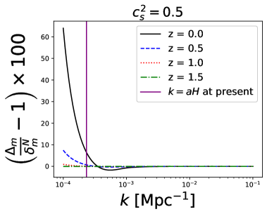
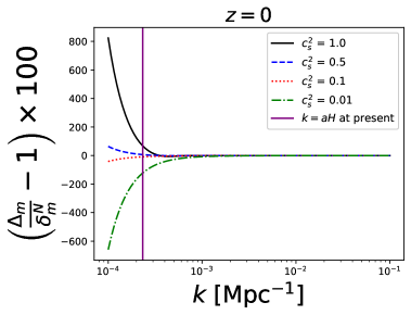
Figure 1: Percentage deviation of the relativistic perturbation results for $\Delta_{m}$ compared to the Newtonian perturbation result for $\delta_{m}^{N}$.

In Figure 1, we have compared the results from relativistic and Newtonian perturbation theory for the matter-energy overdensity contrast. The vertical purple line is for the horizon scale corresponding to $k_{H}(z=0)=a(z=0)H(z=0)\approx 0.00023$ Mpc^-1 for $h=0.7$, where $h$ is related to $H_{0}$ given as

$$H_{0}=100\hskip 5.69046pth\hskip 5.69046pt\text{Km}\hskip 2.84544pt\text{S}^{-1}\hskip 2.84544pt\text{Mpc}^{-1}.$$ (6.3)

We find that for almost all the cases the relativistic perturbation results match well within 10$\%$ with the Newtonian perturbation results for the sub-Hubble scales. We are interested in the sub-Hubble scales, so from now on we shall use the Newtonian perturbation results. The growth factor corresponding to the matter inhomogeneities is given as [73]

$$f=\frac{d\ln D_{+}}{d\ln a}=\frac{T}{\delta_{m}^{N}},$$ (6.4)

where $D_{+}$ is the growing mode solution of $\delta_{m}^{N}$.

In the Newtonian perturbation theory, the normalization factor of the matter power spectrum, $\sigma_{8}$ is independent of the scale $k$ and it is written as [74]

$$\sigma_{8}=\sigma_{8}^{0}\frac{D_{+}(z)}{D_{+}(z=0)}=\sigma_{8}^{0}\frac{\delta_{m}^{N}(z)}{\delta_{m}^{N}(z=0)},$$ (6.5)

where $\sigma_{8}^{0}$ is the present value of $\sigma_{8}$.

7 Observational data

We consider Planck 2018 results of the cosmic microwave background (CMB) observations for the ’TT,TE,EE+lowl+lowE+lensing’ with the base flat $\Lambda$CDM model, where ’T’ stands for temperature in the CMB map and ’E’ stands for E-mode of the CMB polarisation map [11]. For this purpose, in this analysis, we use the CMB distance prior data corresponding to these observations [75, 76]. For the CMB distance prior, we use the corresponding constraints on the CMB shift parameter, acoustic length scale, and the present value of baryon energy density parameter ($\Omega_{\rm b0}$) according to the [76]. We denote this observation as ’CMB’ throughout this analysis.

We consider Pantheon compilation of the type Ia supernova observations which possesses apparent peak absolute magnitudes of the standard candles at different redshift values [7]. This apparent magnitude depends on the value of the luminosity of a source at a particular redshift and the nuisance parameter $M_{B}$. $M_{B}$ is the peak absolute magnitude of a type Ia supernova. We constrain $M_{B}$ alongside the model parameters. We denote this observation as ’SN’.

We consider the cosmic chronometer data for the Hubble parameter at different redshift values [77, 78]. In these observations, the Hubble parameter is determined by the relative galaxy ages. For the Hubble parameter data, we closely follow [78]. We denote this observation as ’CC’.

We consider baryon acoustic oscillations (BAO) data which are related to the cosmological distances like the angular diameter distance. The BAO observations possess data both in the line of sight direction and transverse direction [13]. The line of sight data is related to the Hubble parameter and the transverse data is related to the angular diameter distance [12, 13, 14]. For the BAO data, we follow [13]. However, we exclude the measurement of eBOSS (the extended baryon oscillation spectroscopic survey) emission-line galaxies (ELGs) data from the list in [13] because this data (at redshift, $z=0.8$) have an asymmetric standard deviation in the statistical measurement. Note that BAO observation is dependent on the parameter, $r_{d}$, the distance to the baryon drag epoch. This parameter is closely related to the parameter, $\Omega_{\rm b0}$. So, in our analysis, we constrain this parameter as a nuisance parameter like in the case of CMB data. We denote the BAO observations as ’BAO’.

We also consider the $f\sigma_{8}$ data in our analysis. This data constrains the model parameters both through background and perturbation evolutions. We consider 63 $f\sigma_{8}$ data at different redshift ranging from $z=10^{-3}$ to $z=2$. For these data, we follow [79]. We denote these observations as ’$f\sigma_{8}$’. With all these data, we constrain the model parameters alongside the cosmological nuisance parameters.

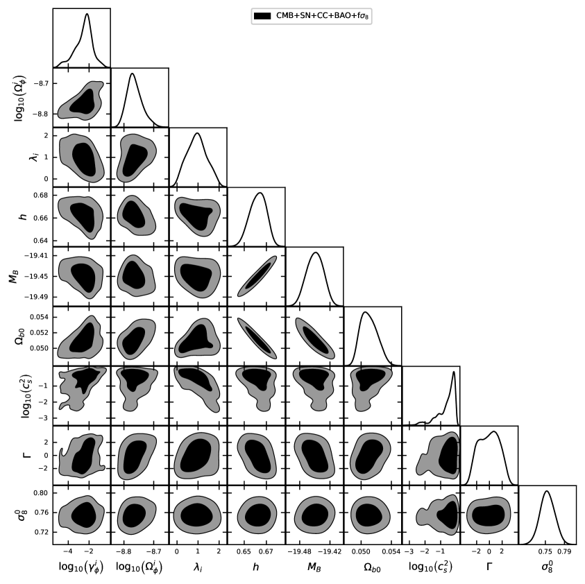
Figure 2: Constraints on all the model parameters obtained from the CMB+SN+CC+BAO+$f\sigma_{8}$ combinations of data. The inner and outer regions correspond to 1$\sigma$ and 2$\sigma$ bounds respectively.

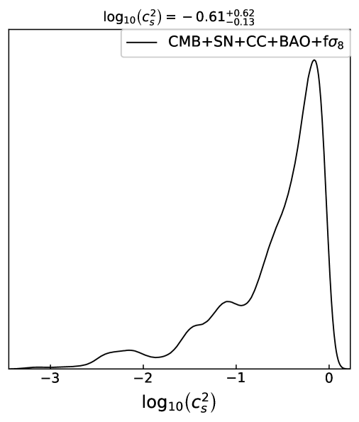
Figure 3: Marginalized probability of $\log_{10}c_{s}^{2}$ obtained from CMB+SN+CC+BAO+$f\sigma_{8}$ combinations of data.

8 Results

Parameters	1$\sigma$ bounds
$\log_{\rm 10}(\gamma_{\phi}^{i})$	$-2.52^{+0.88}_{-0.63}$
$\log_{\rm 10}(\Omega_{\phi}^{i})$	$-8.764^{+0.020}_{-0.029}$
$\lambda_{i}$	$0.94^{+0.45}_{-0.53}$
$h$	$0.6624^{+0.0081}_{-0.0069}$
$M_{B}$	$-19.450\pm 0.016$
$\Omega_{\rm b0}$	$0.05102^{+0.00095}_{-0.0013}$
$\log_{\rm 10}(c_{s}^{2})$	$-0.61^{+0.62}_{-0.13}$
$\Gamma$	$-0.1\pm 1.6$
$\sigma_{8}^{0}$	$0.754\pm 0.015$

Table 1: 1$\sigma$ bounds on all the model parameters obtained from CMB+SN+CC+BAO+$f\sigma_{8}$ combinations of data.

In Figure 2, we have shown constraints on all the parameters obtained from the combined CMB+SN+CC+BAO+$f\sigma_{8}$ data. The inner-darker-black and outer-lighter-black contours correspond to the 1$\sigma$ and 2$\sigma$ contour ellipses respectively. The 1$\sigma$ values of parameters are mentioned in Table 1.

As we can see, from the combinations of all the data, mentioned earlier, the higher values of $c_{s}^{2}$ (close to $1$) are not tightly constrained. But, interestingly, constraints on the lower values of $c_{s}^{2}$ (close to $0$) are tighter. This can also be seen from Figure 3, where we have shown the marginalized probability of $\log_{10}c_{s}^{2}$. This means the homogeneous dark energy is more favorable than the clustering dark energy from the recent observational data, we have considered. This analysis shows tighter constraints on $c_{s}^{2}$ (on the lower side i.e. close to $0$) compared to the results obtained in the earlier studies like in [64, 65, 66, 67, 68, 69]. This is our main highlighted result. However, from the constraints on the different model parameters, we see some other interesting results, mentioned below.

From the constraints on $\gamma_{\phi}^{i}$, we see that its mean value is of the order of $10^{-}2$ which corresponds to the fact that the equation of the state parameter of the dark energy is very close to $-1$ at the initial time. This means the initial condition for the scalar field evolution favors the thawing behavior for a larger set of forms of potential including polynomials and the exponential. Even the negative values of the powers in the polynomial potentials also favor the thawing behaviors which can be seen from the constraints on the $\Gamma$ parameters, in which we see the large range of the parameter space is allowed for $\Gamma$ including $0$ (corresponding to the exponential potential) and positive values (corresponding to the negative power of the polynomial potentials). Note that, these results are only for the polynomial and exponential potentials not for any arbitrary general form of potential.

The results for the constraints on the $H_{0}$ parameter (through the parameter, $h$) are similar to the ones, we expect from the CMB, CC, and BAO observations. Since $M_{B}$ is degenerate to $H_{0}$, constraints on $M_{B}$ are also consistent. The constraints on the $\Omega_{\rm b0}$ are also consistent, as we expect from the CMB and the BAO observations. Similar is the case for the constraints on the $\sigma_{8}^{0}$ parameter.

9 Conclusion

We consider a k-essence model of dark energy in which the sound speed of dark energy is constant. We write down the corresponding Lagrangian for this kind of model. With this Lagrangian, we calculate the Euler-Lagrange equation and the field equations in general. We then set up a dynamical system of differential equations for the background evolutions with the help of dimensionless variables. After numerically solving this autonomous system, we compute the relevant background quantities like the Hubble parameter, the equation of state parameter of the dark energy, and the energy density parameter of the k-essence scalar field.

We also compute the first-order linear perturbations to compute the relevant perturbation quantities like the growth factor and the $\sigma_{8}$. We consider both the relativistic and the Newtonian perturbations and compare them. We find the results match excellent within the sub-Hubble limit. For the evolution of the perturbations, we use dimensionless variables to get an autonomous system of differential equations. We combine this autonomous system with the one for background evolution and make a completely autonomous system of differential equations. From this, we compute all the relevant quantities.

Next, we do the parameter estimation to put constraints on the model parameters as well as on the cosmological nuisance parameters from the combinations of Planck 2018 mission of CMB observations, the Pantheon compilation of type Ia supernova observations, the cosmic chronometers observations for the Hubble parameter, the BAO observations, and the $f\sigma_{8}$ observations.

The mean value of $c_{s}^{2}$ is close to $1$, because the mean value of $\log_{\rm 10}(c_{s}^{2})$ is close to zero which can be seen in Figures 2 and 3. The higher values of $c_{s}^{2}$ (close to $1$) are loosely constrained i.e. it is allowed for large error bars. On the other hand, the lower values of $c_{s}^{2}$ are comparatively tightly constrained to lie far away from the mean value (in the aspect of the confidence interval). This can be seen in Figure 3. This means the homogeneous dark energy models are more favored than the clustering dark energy models with the recent cosmological observations.

Another interesting result, we find, is that the thawing behavior for the initial condition of the scalar field evolution is favorable at least for the polynomial and exponential potentials of the scalar field.

References

- [1] Supernova Cosmology Project Collaboration, S. Perlmutter et al., Discovery of a supernova explosion at half the age of the Universe and its cosmological implications, Nature 391 (1998) 51–54, [astro-ph/9712212].
- [2] Supernova Search Team Collaboration, A. G. Riess et al., Observational evidence from supernovae for an accelerating universe and a cosmological constant, Astron. J. 116 (1998) 1009–1038, [astro-ph/9805201].
- [3] Supernova Cosmology Project Collaboration, S. Perlmutter et al., Measurements of and from 42 high redshift supernovae, Astrophys. J. 517 (1999) 565–586, [astro-ph/9812133].
- [4] A. Wright, Nobel Prize 2011: Perlmutter, Schmidt & Riess, Nature Physics 7 (Nov., 2011) 833.
- [5] S. Linden, J. M. Virey, and A. Tilquin, Cosmological parameter extraction and biases from type ia supernova magnitude evolution, Astronomy and Astrophysics 506 (2009) 1095–1105.
- [6] D. Camarena and V. Marra, A new method to build the (inverse) distance ladder, Mon. Not. Roy. Astron. Soc. 495 (2020), no. 3 2630–2644, [arXiv:1910.14125].
- [7] Pan-STARRS1 Collaboration, D. M. Scolnic et al., The Complete Light-curve Sample of Spectroscopically Confirmed SNe Ia from Pan-STARRS1 and Cosmological Constraints from the Combined Pantheon Sample, Astrophys. J. 859 (2018), no. 2 101, [arXiv:1710.00845].
- [8] A. K. Çamlıbel, I. Semiz, and M. A. Feyizoğlu, Pantheon update on a model-independent analysis of cosmological supernova data, Class. Quant. Grav. 37 (2020), no. 23 235001, [arXiv:2001.04408].
- [9] Planck Collaboration, P. A. R. Ade et al., Planck 2013 results. XVI. Cosmological parameters, Astron. Astrophys. 571 (2014) A16, [arXiv:1303.5076].
- [10] Planck Collaboration, P. A. R. Ade et al., Planck 2015 results. XIII. Cosmological parameters, Astron. Astrophys. 594 (2016) A13, [arXiv:1502.01589].
- [11] Planck Collaboration, N. Aghanim et al., Planck 2018 results. VI. Cosmological parameters, Astron. Astrophys. 641 (2020) A6, [arXiv:1807.06209]. [Erratum: Astron.Astrophys. 652, C4 (2021)].
- [12] BOSS Collaboration, S. Alam et al., The clustering of galaxies in the completed SDSS-III Baryon Oscillation Spectroscopic Survey: cosmological analysis of the DR12 galaxy sample, Mon. Not. Roy. Astron. Soc. 470 (2017), no. 3 2617–2652, [arXiv:1607.03155].
- [13] eBOSS Collaboration, S. Alam et al., Completed SDSS-IV extended Baryon Oscillation Spectroscopic Survey: Cosmological implications from two decades of spectroscopic surveys at the Apache Point Observatory, Phys. Rev. D 103 (2021), no. 8 083533, [arXiv:2007.08991].
- [14] J. Hou et al., The Completed SDSS-IV extended Baryon Oscillation Spectroscopic Survey: BAO and RSD measurements from anisotropic clustering analysis of the Quasar Sample in configuration space between redshift 0.8 and 2.2, Mon. Not. Roy. Astron. Soc. 500 (2020), no. 1 1201–1221, [arXiv:2007.08998].
- [15] P. J. E. Peebles and B. Ratra, The Cosmological Constant and Dark Energy, Rev. Mod. Phys. 75 (2003) 559–606, [astro-ph/0207347].
- [16] E. J. Copeland, M. Sami, and S. Tsujikawa, Dynamics of dark energy, Int. J. Mod. Phys. D 15 (2006) 1753–1936, [hep-th/0603057].
- [17] J. Yoo and Y. Watanabe, Theoretical Models of Dark Energy, Int. J. Mod. Phys. D 21 (2012) 1230002, [arXiv:1212.4726].
- [18] A. I. Lonappan, S. Kumar, Ruchika, B. R. Dinda, and A. A. Sen, Bayesian evidences for dark energy models in light of current observational data, Phys. Rev. D 97 (2018), no. 4 043524, [arXiv:1707.00603].
- [19] B. R. Dinda, Probing dark energy using convergence power spectrum and bi-spectrum, JCAP 09 (2017) 035, [arXiv:1705.00657].
- [20] B. R. Dinda, A. A. Sen, and T. R. Choudhury, Dark energy constraints from the 21~cm intensity mapping surveys with SKA1, arXiv:1804.11137.
- [21] T. Clifton, P. G. Ferreira, A. Padilla, and C. Skordis, Modified Gravity and Cosmology, Phys. Rept. 513 (2012) 1–189, [arXiv:1106.2476].
- [22] K. Koyama, Cosmological Tests of Modified Gravity, Rept. Prog. Phys. 79 (2016), no. 4 046902, [arXiv:1504.04623].
- [23] S. Tsujikawa, Modified gravity models of dark energy, Lect. Notes Phys. 800 (2010) 99–145, [arXiv:1101.0191].
- [24] A. Joyce, L. Lombriser, and F. Schmidt, Dark Energy Versus Modified Gravity, Ann. Rev. Nucl. Part. Sci. 66 (2016) 95–122, [arXiv:1601.06133].
- [25] B. R. Dinda, M. Wali Hossain, and A. A. Sen, Observed galaxy power spectrum in cubic Galileon model, JCAP 01 (2018) 045, [arXiv:1706.00567].
- [26] B. R. Dinda, Weak lensing probe of cubic Galileon model, JCAP 06 (2018) 017, [arXiv:1801.01741].
- [27] J. Zhang, B. R. Dinda, M. W. Hossain, A. A. Sen, and W. Luo, Study of cubic Galileon gravity using -body simulations, Phys. Rev. D 102 (2020), no. 4 043510, [arXiv:2004.12659].
- [28] B. R. Dinda, M. W. Hossain, and A. A. Sen, 21 cm power spectrum in interacting cubic Galileon model, arXiv:2208.11560.
- [29] A. Bassi, B. R. Dinda, and A. A. Sen, 21 cm Power Spectrum for Bimetric Gravity and its Detectability with SKA1-Mid Telescope, arXiv:2306.03875.
- [30] S. M. Carroll, The Cosmological constant, Living Rev. Rel. 4 (2001) 1, [astro-ph/0004075].
- [31] I. Zlatev, L.-M. Wang, and P. J. Steinhardt, Quintessence, cosmic coincidence, and the cosmological constant, Phys. Rev. Lett. 82 (1999) 896–899, [astro-ph/9807002].
- [32] V. Sahni and A. A. Starobinsky, The Case for a positive cosmological Lambda term, Int. J. Mod. Phys. D 9 (2000) 373–444, [astro-ph/9904398].
- [33] H. Velten, R. vom Marttens, and W. Zimdahl, Aspects of the cosmological “coincidence problem”, Eur. Phys. J. C 74 (2014), no. 11 3160, [arXiv:1410.2509].
- [34] M. Malquarti, E. J. Copeland, and A. R. Liddle, K-essence and the coincidence problem, Phys. Rev. D 68 (2003) 023512, [astro-ph/0304277].
- [35] E. Di Valentino, O. Mena, S. Pan, L. Visinelli, W. Yang, A. Melchiorri, D. F. Mota, A. G. Riess, and J. Silk, In the Realm of the Hubble tension a Review of Solutions, arXiv:2103.01183.
- [36] C. Krishnan, R. Mohayaee, E. O. Colgáin, M. M. Sheikh-Jabbari, and L. Yin, Does Hubble tension signal a breakdown in FLRW cosmology?, Class. Quant. Grav. 38 (2021), no. 18 184001, [arXiv:2105.09790].
- [37] S. Vagnozzi, New physics in light of the tension: An alternative view, Phys. Rev. D 102 (2020), no. 2 023518, [arXiv:1907.07569].
- [38] B. R. Dinda, Cosmic expansion parametrization: Implication for curvature and H0 tension, Phys. Rev. D 105 (2022), no. 6 063524, [arXiv:2106.02963].
- [39] E. Di Valentino et al., Cosmology Intertwined III: and , Astropart. Phys. 131 (2021) 102604, [arXiv:2008.11285].
- [40] E. Abdalla et al., Cosmology intertwined: A review of the particle physics, astrophysics, and cosmology associated with the cosmological tensions and anomalies, JHEAp 34 (2022) 49–211, [arXiv:2203.06142].
- [41] M. Douspis, L. Salvati, and N. Aghanim, On the Tension between Large Scale Structures and Cosmic Microwave Background, PoS EDSU2018 (2018) 037, [arXiv:1901.05289].
- [42] A. Bhattacharyya, U. Alam, K. L. Pandey, S. Das, and S. Pal, Are and tensions generic to present cosmological data?, Astrophys. J. 876 (2019), no. 2 143, [arXiv:1805.04716].
- [43] R. de Putter, D. Huterer, and E. V. Linder, Measuring the speed of dark: Detecting dark energy perturbations, Phys. Rev. D 81 (May, 2010) 103513.
- [44] C. Armendariz-Picon, V. F. Mukhanov, and P. J. Steinhardt, Essentials of k essence, Phys. Rev. D 63 (2001) 103510, [astro-ph/0006373].
- [45] C. Armendariz-Picon, V. F. Mukhanov, and P. J. Steinhardt, A Dynamical solution to the problem of a small cosmological constant and late time cosmic acceleration, Phys. Rev. Lett. 85 (2000) 4438–4441, [astro-ph/0004134].
- [46] C. Armendariz-Picon, T. Damour, and V. F. Mukhanov, k - inflation, Phys. Lett. B 458 (1999) 209–218, [hep-th/9904075].
- [47] R.-J. Yang, B. Chen, J. Li, and J. Qi, The evolution of the power law k-essence cosmology, Astrophys. Space Sci. 356 (2015), no. 2 399–405, [arXiv:1311.5307].
- [48] V. H. Cárdenas, N. Cruz, and J. R. Villanueva, Testing a dissipative kinetic k-essence model, Eur. Phys. J. C 75 (2015), no. 4 148, [arXiv:1503.03826].
- [49] S. Mukherjee and D. Gangopadhyay, An accelerated universe with negative equation of state parameter in inhomogeneous cosmology with -essence scalar field, Phys. Dark Univ. 32 (2021) 100800, [arXiv:1602.01289].
- [50] A. Chakraborty, A. Ghosh, and N. Banerjee, Dynamical systems analysis of a k -essence model, Phys. Rev. D 99 (2019), no. 10 103513, [arXiv:1904.10149].
- [51] R. Gannouji and Y. R. Baez, Critical collapse in K-essence models, JHEP 07 (2020) 132, [arXiv:2003.13730].
- [52] D. Perkovic and H. Stefancic, Purely kinetic k-essence description of barotropic fluid models, Phys. Dark Univ. 32 (2021) 100827, [arXiv:2009.08680].
- [53] Z. Huang, Statistics of thawing k-essence dark energy models, Phys. Rev. D 104 (2021), no. 10 103533, [arXiv:2108.06089].
- [54] A. Chatterjee, B. Jana, and A. Bandyopadhyay, Modified scaling in k-essence model in interacting dark energy–dark matter scenario, Eur. Phys. J. Plus 137 (2022), no. 11 1271, [arXiv:2207.00888].
- [55] B. Ratra and P. J. E. Peebles, Cosmological consequences of a rolling homogeneous scalar field, Phys. Rev. D 37 (Jun, 1988) 3406–3427.
- [56] A. R. Liddle and R. J. Scherrer, A Classification of scalar field potentials with cosmological scaling solutions, Phys. Rev. D 59 (1999) 023509, [astro-ph/9809272].
- [57] P. J. Steinhardt, L.-M. Wang, and I. Zlatev, Cosmological tracking solutions, Phys. Rev. D 59 (1999) 123504, [astro-ph/9812313].
- [58] R. R. Caldwell and E. V. Linder, The Limits of quintessence, Phys. Rev. Lett. 95 (2005) 141301, [astro-ph/0505494].
- [59] R. J. Scherrer and A. A. Sen, Thawing quintessence with a nearly flat potential, Phys. Rev. D 77 (2008) 083515, [arXiv:0712.3450].
- [60] B. R. Dinda and A. A. Sen, Imprint of thawing scalar fields on the large scale galaxy overdensity, Phys. Rev. D 97 (2018), no. 8 083506, [arXiv:1607.05123].
- [61] K. Bamba, J. Matsumoto, and S. Nojiri, Cosmological perturbations in -essence model, Phys. Rev. D 85 (2012) 084026, [arXiv:1109.1308].
- [62] J. Matsumoto, Cosmological Linear Perturbations in the Models of Dark Energy and Modified Gravity, Universe 1 (2015), no. 1 17–23, [arXiv:1401.3077].
- [63] B. R. Dinda, Nonlinear power spectrum in clustering and smooth dark energy models beyond the BAO scale, J. Astrophys. Astron. 40 (2019), no. 2 12, [arXiv:1804.07953].
- [64] O. Sergijenko and B. Novosyadlyj, Sound speed of scalar field dark energy: weak effects and large uncertainties, Phys. Rev. D 91 (2015), no. 8 083007, [arXiv:1407.2230].
- [65] M. Kunz, S. Nesseris, and I. Sawicki, Using dark energy to suppress power at small scales, Phys. Rev. D 92 (2015), no. 6 063006, [arXiv:1507.01486].
- [66] M. Bouhmadi-López, K. S. Kumar, J. Marto, J. Morais, and A. Zhuk, -essence model from the mechanical approach point of view: coupled scalar field and the late cosmic acceleration, JCAP 07 (2016) 050, [arXiv:1605.03212].
- [67] S. Hannestad, Constraints on the sound speed of dark energy, Phys. Rev. D 71 (2005) 103519, [astro-ph/0504017].
- [68] E. Majerotto, D. Sapone, and B. M. Schäfer, Combined constraints on deviations of dark energy from an ideal fluid from Euclid and Planck, Mon. Not. Roy. Astron. Soc. 456 (2016), no. 1 109–118, [arXiv:1506.04609].
- [69] J.-Q. Xia, Y.-F. Cai, T.-T. Qiu, G.-B. Zhao, and X. Zhang, Constraints on the Sound Speed of Dynamical Dark Energy, Int. J. Mod. Phys. D 17 (2008) 1229–1243, [astro-ph/0703202].
- [70] M. Malquarti, E. J. Copeland, A. R. Liddle, and M. Trodden, A New view of k-essence, Phys. Rev. D 67 (2003) 123503, [astro-ph/0302279].
- [71] L. P. Chimento and A. Feinstein, Power - law expansion in k-essence cosmology, Mod. Phys. Lett. A 19 (2004) 761–768, [astro-ph/0305007].
- [72] P. Jorge, J. P. Mimoso, and D. Wands, On the dynamics of k-essence models, Journal of Physics: Conference Series 66 (may, 2007) 012031.
- [73] D. Huterer et al., Growth of Cosmic Structure: Probing Dark Energy Beyond Expansion, Astropart. Phys. 63 (2015) 23–41, [arXiv:1309.5385].
- [74] E. Pierpaoli, D. Scott, and M. J. White, Power spectrum normalization from the local abundance of rich clusters of galaxies, Mon. Not. Roy. Astron. Soc. 325 (2001) 77, [astro-ph/0010039].
- [75] Z. Zhai and Y. Wang, Robust and model-independent cosmological constraints from distance measurements, JCAP 07 (2019) 005, [arXiv:1811.07425].
- [76] L. Chen, Q.-G. Huang, and K. Wang, Distance Priors from Planck Final Release, JCAP 02 (2019) 028, [arXiv:1808.05724].
- [77] A. M. Pinho, S. Casas, and L. Amendola, Model-independent reconstruction of the linear anisotropic stress , JCAP 11 (2018) 027, [arXiv:1805.00027].
- [78] R. Jimenez and A. Loeb, Constraining cosmological parameters based on relative galaxy ages, Astrophys. J. 573 (2002) 37–42, [astro-ph/0106145].
- [79] L. Kazantzidis and L. Perivolaropoulos, Evolution of the tension with the Planck15/CDM determination and implications for modified gravity theories, Phys. Rev. D 97 (2018), no. 10 103503, [arXiv:1803.01337].