CERN-TH-2023-131

Higgs boson pair production at NLO in the Powheg approach and the top quark mass uncertainties

Emanuele Bagnaschi^a,b, Giuseppe Degrassi^c, Ramona Gröber^d
(a) Istituto Nazionale di Fisica Nucleare, Laboratori Nazionali di Frascati, C.P. 13, 00044 Frascati, Italy
(b) CERN, Theoretical Physics Department, 1211 Geneva 23, Switzerland
(c) Dipartimento di Matematica e Fisica, Università di Roma Tre and
INFN, sezione di Roma Tre, I-00146 Rome, Italy
(d) Dipartimento di Fisica e Astronomia ’G. Galilei’, Università di Padova and INFN, sezione di Padova, I-35131 Padova, Italy

We present a new Monte Carlo code for Higgs boson pair production at next-to-leading order in the Powheg-Box Monte Carlo approach. The code is based on analytic results for the two loop virtual corrections which include the full top quark mass dependence. This feature allows to freely assign the value of all input parameters, including the trilinear Higgs boson self coupling, as well as to vary the renormalization scheme employed for the top quark mass. We study the uncertainties due to the top-mass renormalization scheme allowing the trilinear Higgs boson self coupling to vary around its Standard Model value including parton shower effects. Results are presented for both inclusive and differential observables.

1 Introduction

With the discovery of the Higgs boson [1, 2] the study of its potential and self-interactions has become of great interest to the scientific community as an ultimate probe of the mechanism of electroweak symmetry breaking.

In the Standard Model (SM), the Higgs potential in the unitary gauge reads

$$V(H)=\frac{m_{\scriptscriptstyle H}^{2}}{2}H^{2}+\lambda_{3}vH^{3}+\frac{\lambda_{4}}{4}H^{4},$$ (1)

where the Higgs mass ($m_{\scriptscriptstyle H}$) and the trilinear $(\lambda_{3})$ and quartic $(\lambda_{4})$ interactions are linked by the relations $\lambda_{4}^{\rm SM}=\lambda_{3}^{\rm SM}=\lambda=m_{\scriptscriptstyle H}^{2}/(2\,v^{2})$, where $v=(\sqrt{2}\,G_{\mu})^{-1/2}$ is the vacuum expectation value, $G_{\mu}$ the Fermi constant and $\lambda$ is the coefficient of the $(\Phi^{\dagger}\Phi)^{2}$ interaction, $\Phi$ being the Higgs doublet field.

The Higgs mass has now been measured at the level of  one per mille precision [3, 4]. The trilinear Higgs self-coupling is hence predicted within the SM and its determination at the Large Hadron Collider (LHC), where it is accessible via the production of Higgs boson pairs, thus provides a probe of the SM. However, the main production mode, gluon fusion, has a very small SM cross-section [5] and sensitivity to the $\lambda_{3}$ SM value has not yet been reached, so that only constraints on $\lambda_{3}$ can be derived for now. However, during the recent years, the interval of allowed values for $\lambda_{3}$ has shrunk significantly and this trend will continue during Run 3 and the High-Luminosity (HL) phase of the LHC. Presently, from the analyses of the decay channels, $HH\to b\bar{b}\gamma\gamma,\>HH\to b\bar{b}\tau\tau$ and $HH\to b\bar{b}b\bar{b}$, the ATLAS Collaboration excluded values outside the interval $-0.6<\kappa_{\lambda}<6.6$, where $\kappa_{\lambda}=\lambda_{3}/\lambda_{3}^{\rm SM}$, at 95% confidence level (CL) under the assumption that all the other couplings have SM values [6]. A slightly stronger limit can be obtained by combining the information from double Higgs production with the one coming from other processes that are sensitive to $\lambda_{3}$ via next-to-leading order (NLO) electroweak (EW) corrections [8, 9, 10, 11, 12, 13, 14, 15, 16, 17, 18, 19]. Indeed the combination of the information coming from double-Higgs and single-Higgs production yields $-0.4<\kappa_{\lambda}<6.3$ at 95% CL [6].

In view of future improvements in the experimental analyses of the Higgs pair production process it is interesting to reappraise the uncertainties in the theoretical prediction of this process. The process is mediated by heavy quarks loops that appear in different topologies: i) the “signal” topology given by triangular diagrams which represent the gluon-fusion production of an off-shell Higgs that then subsequently decays via the trilinear coupling into two on-shell bosons and are therefore sensitive to $\lambda_{3}$; ii) the “background” topology that at the leading order (LO) is given by box-like diagrams that do not depend on $\lambda_{3}$. The LO calculation of the Higgs boson pair production has been performed more than thirty years ago [20, 21, 22]. The NLO QCD corrections were first computed in the infinite top mass, $m_{t}$, limit (HTL) [23], reweighted by the exact Born amplitude. Later they were supplemented by the inclusion of $(1/m_{t}^{2})^{n}$ corrections up to $n=6$ [24, 25, 26]. Then the HTL evaluation was retained only in the virtual two-loop corrections, while the real ones were computed including the full top mass dependence [27, 28]. Finally, the full top mass dependence in the virtual correction was obtained by numerical methods [29, 30, 31, 32]. At the same time analytic results for the two-loop virtual corrections, valid in specific regions of the phase space, were presented [33, 34, 35, 36]. The analytic evaluation of the corrections via a high-energy (HE) expansion was later used to replace the numerical evaluation of Refs. [29, 30] in the high-energy region in order to better cover that energy range [37]. Later the HE evaluation was also merged with the analytic evaluation of the corrections via a Higgs transverse momomentum, $p_{\scriptscriptstyle T}$, in order to obtain an analytic result that covers the entire phase space [38].

The NLO fixed order calculation with the full top mass dependence was also matched to parton shower programs [39, 40] and combined with next-to-next-to-leading order (NNLO) QCD corrections in the HTL limit [41, 42, 43, 44] while keeping the double real corrections in full top mass dependence [45]. Results at $\text{N}^{3}\text{LO}$ are available in the HTL [46, 47].

The aim of this paper is twofold. On the one side, we present a new Monte Carlo (MC) code for Higgs pair production in the Powheg-Box approach [48, 49]. The code retains the full top quark mass dependence at NLO and is flexible in the input parameters. In our code it is possible to vary at the same time both the top mass scheme used and the value of $\lambda_{3}$. This is achieved employing an analytic result for the virtual two-loop corrections instead of a numerical grid as in the MC code of Refs. [39, 50]. On the other side, we study the uncertainty related to the renormalization scheme used for the top mass for arbitrary values of the trilinear coupling including parton shower effects.

With respect to previous works in the literature where similar analyses were presented our work contains several improvements. In Ref. [50] the dependence on $\lambda_{3}$ of the Higgs pair total cross section and differential distributions was studied including parton shower effects. We improve this analysis by addressing also the dependence on the top mass renormalization scheme. The uncertainties in double Higgs production related to the top mass scheme were analyzed in Refs. [31, 32, 51]. With respect to these studies, that are based on a NLO fixed order calculation, we improved the analysis by including parton shower effects. Furthermore, these previous studies were concentrating on the investigation of the total cross section or the differential cross section as a function of the Higgs-pair invariant mass, $M_{HH}$, while we have the possibility to study other differential distributions.

In this paper we do not discuss the technical details of our MC code. They can be found in the instruction manual in the Docs directory of the source code tree. The code will be available on the Powheg-Box repository at https://powhegbox.mib.infn.it.

The paper is organized as follows. In section 2 we describe the basic feature of our Powheg implementation of the $gg\to HH$ process. In section 3 we present our results for the inclusive cross section and differential distributions using different top-quark-mass renormalization schemes and for several values of $\lambda_{3}$. We will also compare our results with those of previous analyses. Finally we present our conclusions.

2 Powheg implementation of $gg\rightarrow HH$

In this section we briefly discuss the main characteristics of our implementation of the gluon-fusion Higgs pair production process in the Powheg-Box framework. We first briefly recall the basic features of the Powheg formalism, and the required elements to implement a process in the Powheg-Box framework. We then discuss in more detail our implementation of the virtual two-loop corrections and of the real radiation contributions. The way how these two contributions are implemented is the main difference between our MC code and the one presented in Refs. [39, 50].

2.1 The Powheg approach

The Powheg formula to match NLO-QCD accurate calculations with parton showers can be written in a sufficiently general way as

$$d\sigma=\bar{B}^{s}(\Phi_{B})d\Phi_{B}\left\{\Delta^{s}_{t_{0}}+\Delta^{s}_{t}\frac{R^{s}(\Phi)}{B(\Phi_{B})}d\Phi_{r}\right\}+R^{f}(\Phi)d\Phi+R^{\text{reg}}(\Phi)d\Phi.$$ (2)

The Born squared matrix element is represented as $B(\Phi_{B})$, with $\Phi_{B}$ being the phase space at the leading order. The squared matrix elements of the real emission, i.e. channels with an additional parton with respect to the Born process, can be divided in two sets, according to whether they feature soft/collinear divergences, in which case we denote them as $R^{\text{div}}(\Phi)$, or not, $R^{\text{reg}}(\Phi)$. $\Phi$ represents the product of the Born and the real emission phase spaces $\Phi=\Phi_{B}\Phi_{r}$. In the Powheg-Box framework it is possible to split the contribution from the divergent processes $R^{\text{div}}(\Phi)$ into two terms, $R^{s}(\Phi)$ and $R^{f}(\Phi)$. The term $R^{s}$ should contain the singular terms, and it is matched with the parton shower using the Powheg Sudakov form factor $\Delta^{s}_{t}$. The definition of the latter is

$$\Delta^{s}_{t}=e^{-\int\frac{dt^{\prime}}{t^{\prime}}\frac{R^{s}}{B}d\Phi_{r}\theta(t^{\prime}-t)}\,,$$ (3)

with $t$ being the shower ordering variable. The $t_{0}$ appearing in eq. (2) is a lower-scale cutoff. On the other hand, $R^{f}$, which should be finite, is simply added as shown in eq. (2), without any further treatment. The arbitrariness in choosing $R^{f}$ can be used to study the theoretical uncertainties linked to the matching procedure, since different definitions differ by higher-order terms. The non-divergent channels, $R^{\text{reg}}$, are also added without being multiplied by the Powheg Sudakov form factor. Finally, the $\bar{B}^{s}(\Phi_{B})$ is the NLO normalization factor

$$\bar{B}^{s}(\Phi_{B})=B(\Phi_{B})+\hat{V}_{\text{fin}}(\Phi_{B})+\int\hat{R}^{s}(\Phi_{B},\Phi_{r})d\Phi_{r}\,.$$ (4)

In this formula, $\hat{V}_{\text{fin}}$ represents IR- and UV-regularized two-loop virtual contribution, while $\hat{R}^{s}$ is the IR-subtracted real contribution as defined above.

In our MC code $B(\Phi_{B})$ is obtained from Ref. [20] where the LO amplitude is presented in terms of the Passarino-Veltman functions [52]. The evaluation of the latters is performed using the COLLIER code [53].

2.2 Virtual two-loop contribution

The virtual two-loop diagrams, that enter in $\hat{V}_{\text{fin}}(\Phi_{B})$, can be assigned to “signal” and “background” topologies as in the LO case. The contribution of the “signal” diagrams (triangular topology) is known analytically including the full top mass dependence adapting results for the production of a single Higgs with virtuality $M_{HH}$ [54, 55]. In our code we implement the expressions of Ref. [54]. The possibility of varying the trilinear coupling is introduced via an additional parameter that rescales the “signal” contribution.

The “background” topologies are of two types: double-triangle and box diagrams. Concerning the former, the diagram topology is the product of two one-loop triangle diagrams and we implement in our code the analytic results derived in Ref.[26] that retain the full top mass dependence. The box diagrams are the most difficult contribution to evaluate. The box diagrams depend on four energy scales, namely $\hat{s},\,\hat{t},\,m_{t},m_{\scriptscriptstyle H}$, where $\hat{s},\,\hat{t}$, and $\hat{u}$ are the Mandelstam variables which satisfy the condition

$$\hat{s}+\hat{t}+\hat{u}=2\,m_{\scriptscriptstyle H}^{2}~{}.$$ (5)

Alternatively, the scale $\hat{t}$ can be replaced by the transverse momentum of the Higgs particle, $p_{\scriptscriptstyle T}$. Exact analytic results for two-loop box diagrams with several energy scales is at the verge of what can be obtained with the present computational technology. However, using the method of the expansion of the diagrams in terms of ratios of small energy scales vs. large energy scales, it is possible to obtain an analytic evaluation of these diagrams that is valid in specific regions of the phase space where an hierarchy among the various energy scales present in the diagrams is realized. The method of the expansion in terms of the transverse momentum of the Higgs boson [33] is valid in phase-space regions where $|\hat{t}|/(4m_{t}^{2})\lesssim 1$ while the high-energy (HE) expansion method [35] covers the complementary regions of the phase space where $|\hat{t}|/(4m_{t}^{2})\gtrsim 1$. In the $p_{\scriptscriptstyle T}$ expansion it is assumed that the scales associated to $m_{H}$ and to $p_{\scriptscriptstyle T}$ are small compared to the scales set by $\hat{s}$ and $m_{t}$. Under this assumption, the box integrals are expanded in ratios of small over large scales, and the resulting simplified integrals are written as linear combinations of 52 master integrals (MI) using Integration-by-Parts (IBP) identities obtained with LiteRed [56, 57]. Among the 52 MI, fifty can be expressed in terms of generalised harmonic polylogarithms while two are elliptic integrals [58]. On the other hand, in the HE expansion the two-loop box integrals are first expanded in terms of small $m_{\scriptscriptstyle H}$, then an IBP reduction is performed on the expanded integrals; the resulting MIs are further expanded in the limit $m_{t}^{2}\ll\hat{s},|\hat{t}|$ and expressed in terms of harmonic polylogarithms.

As shown in Ref. [38], in order to merge the two analytic approximations the fixed-order results both in the $p_{\scriptscriptstyle T}$ expansion and in the HE expansion have to be extended up to or beyond their border of validity, i.e. $\hat{t}\simeq 4m_{t}^{2}$, by constructing a [1/1] Padé approximant for the $p_{\scriptscriptstyle T}$ expanded result and a [6/6] Padé approximant for the HE-result. This procedure reproduces the numerical values [59] in the grid of Ref. [37], which is implemented in the MC code presented in Refs. [39, 50], with an accuracy below the $1\%$ level.

In our MC code the two-loop box contribution is implemented via the analytic expressions of the first three terms in the $p_{\scriptscriptstyle T}$–expansion and of the first thirteen terms in the HE–expansion. With the former terms we construct the [1,1] $p_{\scriptscriptstyle T}$–Padé approximant whose expression is evaluated when a point in the phase space satisfies $|\hat{t}|/(4m_{t}^{2})<1$ or $|\hat{u}|/(4m_{t}^{2})<1$. With the latter terms we construct a [6,6] HE–Padé approximant whose expression is evaluated when a point in the phase space lies in the complementary region, $|\hat{t}|/(4m_{t}^{2})\geq 1$ and $|\hat{u}|/(4m_{t}^{2})>1$. The evaluation of the (generalised) harmonic polylogarithms is done using the code handyG [60], while the elliptic integrals are evaluated using the routines of Ref. [61].

Finally, our analytic expressions allow to easily change the renormalization scheme employed for the top mass as discussed in Ref.[38]. Our results are presented in the on-shell (OS) and the modified minimal subtraction ($\overline{\mathrm{MS}}$) top-mass scheme. In particular, for evaluating the top mass in the $\overline{\mathrm{MS}}$ scheme, we first convert the OS mass to $m_{t}^{\overline{\mathrm{MS}}}(\mu_{t}=m_{t}^{\textrm{OS}})$ using the two-loop relation[62], and then run it at two-loop order numerically to the indicated scale $\mu_{t}$ [63].

2.3 Real radiation contribution

As already discussed in subsection 2.1, in the Powheg-Box framework the real emission channels are assigned to the $R^{\text{div}}$ or $R^{\text{reg}}$ groups, depending on whether they feature soft/collinear-divergent behavior or not.

In double Higgs production in gluon fusion, the $gg\to hhg$ and $gq\to hhq$ channels belong to $R^{\text{div}}$, while the $q\bar{q}\to hhg$ channel belongs to $R^{\text{reg}}$.

The implementation of these channels has been achieved using the MadLoop matrix element generator [64]. The code generated by MadLoop is interfaced directly with the Powheg-Box. The SM model file shipped with MadLoop has been modified in such a way to include an additional parameter that allows for a rescaling of the Higgs trilinear coupling.

To study the uncertainties in the matching of the NLO calculation with parton showers we use the possibility given by the Powheg-Box framework to split the contribution of the processes in $R^{\text{div}}$ into a singular and a finite contribution, respectively $R^{s}$ and $R^{f}$. The events that contribute to the $R^{f}$ term are called “remnant events”.

The separation of $R^{\text{div}}$ in $R^{s}$ and $R^{f}$ is achieved dynamically by using a damping factor, $D_{h}$, via

$$R^{s}=D_{h}~{}R_{\text{div}}~{},\phantom{aaaaaaaaaaa}R^{f}=\left(1-D_{h}\right)~{}R_{\text{div}}\,.$$ (6)

with

$$D_{h}=\frac{h^{2}}{h^{2}+(p_{\bot}^{HH})^{2}}\,,$$ (7)

where $p_{\bot}^{HH}$ is the transverse momentum of the two-Higgs system, and the default value in Powheg for $h$ is $h=\infty$.

Once this separation has been performed, another freedom present in the Powheg-Box framework is the choice of the shower scale for the remnant events (we recall that varying this scale is a higher order effect). By default this scale is set to the $p_{T}$ of the radiated parton. However, it has been found during the study of single Higgs production in gluon fusion [65, 66], that such a choice yields, at large $p_{T}$, harder tails for the NLO system with respect to the fixed order result. To recover the fixed order behavior, it is possible to choose lower scales, in order to limit the phase space available for further emissions by the shower.

We conclude this section by comparing the performance of our MC code with that of the code ggHH presented in Ref. [50]. In the latter the virtual two-loop corrections are implemented via several numerical grids [59] in the Mandelstam variables $\hat{s}$ and $\hat{t}$ for fixed values of the top and Higgs mass and $\alpha_{s}$. An interpolation framework is also provided in order to produce the virtual two-loop amplitude at any point in the phase space. This procedure is faster than our approach to compute the corrections at any point in the phase space via our analytic result. However, it lacks flexibility in the input parameters and, in some regions of the phase space, sometimes the interpolated result is not very accurate [67].

On the contrary, for what concern the real emission contributions our MC code is faster than ggHH. This is due to the different way these contributions are computed. We use the MadLoop code to compute the real radiation matrix elements while in ggHH the same contribution is computed using the GoSam code [68, 69].

The net result of these two competing factors is that our MC has an average timing for evaluating one phase-space point slightly shorter than the corresponding timing in ggHH.

3 Results

In this section, we present our numerical results for a center-of-mass energy $\sqrt{s}=13.6\text{ TeV}$. The values of the input parameters are chosen according to the latest recommendation of the LHC Higgs Working Group (LHCHWG):

$$m_{t}^{\textrm{OS}}=\,172.5~{}\mathrm{GeV},\quad\quad m_{W}=80.385\,\mathrm{GeV},\quad\quad m_{H}=125\,\mathrm{GeV},$$

$$G_{\mu}=1.1663787\times 10^{-5}\,{\mathrm{GeV}^{-2}}\,.$$ (8)

For our studies we adopt the NNPDF31_nlo_as_0118 [70] parton distribution functions (PDF) in a five flavour scheme as reference PDF set for the NLO calculation. Correspondingly, the LO results are obtained using the same set extracted at LO. The value of strong coupling constant is set to be the same as the one used in the PDF, i.e. $\alpha_{s}(M_{Z})=0.118$.

3.1 Inclusive Cross Section

In Table 1, we show the total cross section at 13.6 TeV at LO and NLO for several values of $\lambda_{3}$ adopting different top-quark-mass renormalization schemes, i.e. OS and $\overline{\mathrm{MS}}$ with different scale choices $\mu_{t}$. The values of the renormalization and factorization scales are fixed to be $\mu_{C}=M_{HH}/2$ and the scale uncertainty is estimated from the envelope of a 7-point rescaling of $\mu_{C}$ according to $(\mu_{R}/\mu_{C},\mu_{F}/\mu_{C})=(1,1),(1,\frac{1}{2}),(1,2),(\frac{1}{2},\frac{1}{2}),(\frac{1}{2},1),(2,1),(2,2)$.

$\lambda_{3}/\lambda_{3}^{\rm SM}$	Top-mass scheme	LO [fb]	$\sigma_{LO}/\sigma_{LO}^{OS}$	NLO [fb]	$\sigma_{NLO}/\sigma_{NLO}^{OS}$
-0.6	On-Shell	$55.76_{-21.0\%}^{28.7\%}$	-	$100.77_{-13.7\%}^{15.8\%}$	-
-0.6	$\overline{\mathrm{MS}},\mu_{t}=M_{HH}/4$	$53.52_{-20.9\%}^{28.6\%}$	0.96	$98.52_{-13.9\%}^{16.2\%}$	0.98
-0.6	$\overline{\mathrm{MS}},\mu_{t}=M_{HH}/2$	$54.48_{-20.8\%}^{28.5\%}$	0.98	$99.14_{-13.8\%}^{16.1\%}$	0.98
-0.6	$\overline{\mathrm{MS}},\mu_{t}=M_{HH}$	$55.21_{-20.7\%}^{28.3\%}$	0.99	$99.63_{-13.7\%}^{16.1\%}$	0.99
-0.6	$\overline{\mathrm{MS}},\mu_{t}=m_{t}^{\overline{\mathrm{MS}}}(m_{t}^{\overline{\mathrm{MS}}})$	$56.68_{-20.9\%}^{28.5\%}$	1.02	$101.07_{-13.5\%}^{15.5\%}$	1.00
0	On-Shell	$38.50_{-21.1\%}^{28.9\%}$	-	$68.38_{-13.4\%}^{15.1\%}$	-
0	$\overline{\mathrm{MS}},\mu_{t}=M_{HH}/4$	$36.65_{-21.0\%}^{28.8\%}$	0.95	$66.52_{-13.7\%}^{15.8\%}$	0.97
0	$\overline{\mathrm{MS}},\mu_{t}=M_{HH}/2$	$36.75_{-20.9\%}^{28.7\%}$	0.95	$66.40_{-13.7\%}^{15.8\%}$	0.97
0	$\overline{\mathrm{MS}},\mu_{t}=M_{HH}$	$36.70_{-20.8\%}^{28.5\%}$	0.95	$66.30_{-13.7\%}^{15.9\%}$	0.97
0	$\overline{\mathrm{MS}},\mu_{t}=m_{t}^{\overline{\mathrm{MS}}}(m_{t}^{\overline{\mathrm{MS}}})$	$38.48_{-21.0\%}^{28.7\%}$	1.00	$67.87_{-13.3\%}^{15.1\%}$	0.99
1	On-Shell	$18.22_{-21.3\%}^{29.5\%}$	-	$30.93_{-12.7\%}^{13.7\%}$	-
1	$\overline{\mathrm{MS}},\mu_{t}=M_{HH}/4$	$16.94_{-21.3\%}^{29.3\%}$	0.93	$29.68_{-13.2\%}^{14.7\%}$	0.96
1	$\overline{\mathrm{MS}},\mu_{t}=M_{HH}/2$	$16.22_{-21.2\%}^{29.1\%}$	0.89	$28.90_{-13.5\%}^{15.2\%}$	0.93
1	$\overline{\mathrm{MS}},\mu_{t}=M_{HH}$	$15.48_{-21.1\%}^{29.0\%}$	0.85	$28.27_{-13.9\%}^{16.1\%}$	0.91
1	$\overline{\mathrm{MS}},\mu_{t}=m_{t}^{\overline{\mathrm{MS}}}(m_{t}^{\overline{\mathrm{MS}}})$	$17.30_{-21.2\%}^{29.2\%}$	0.95	$29.78_{-13.0\%}^{14.3\%}$	0.96
2.4	On-Shell	$7.68_{-21.3\%}^{29.3\%}$	-	$13.41_{-13.1\%}^{14.8\%}$	-
2.4	$\overline{\mathrm{MS}},\mu_{t}=M_{HH}/4$	$7.01_{-21.2\%}^{29.1\%}$	0.91	$12.84_{-13.8\%}^{16.3\%}$	0.96
2.4	$\overline{\mathrm{MS}},\mu_{t}=M_{HH}/2$	$6.43_{-21.1\%}^{28.9\%}$	0.84	$12.42_{-14.6\%}^{17.7\%}$	0.93
2.4	$\overline{\mathrm{MS}},\mu_{t}=M_{HH}$	$6.00_{-21.0\%}^{28.7\%}$	0.78	$12.07_{-15.1\%}^{18.5\%}$	0.90
2.4	$\overline{\mathrm{MS}},\mu_{t}=m_{t}^{\overline{\mathrm{MS}}}(m_{t}^{\overline{\mathrm{MS}}})$	$6.92_{-21.1\%}^{29.1\%}$	0.90	$12.81_{-14.1\%}^{16.3\%}$	0.96
6.6	On-Shell	$101.00_{-20.2\%}^{27.4\%}$	-	$203.91_{-15.2\%}^{19.0\%}$	-
6.6	$\overline{\mathrm{MS}},\mu_{t}=M_{HH}/4$	$100.81_{-20.2\%}^{27.4\%}$	1.00	$203.90_{-15.2\%}^{19.1\%}$	1.00
6.6	$\overline{\mathrm{MS}},\mu_{t}=M_{HH}/2$	$109.75_{-20.2\%}^{27.4\%}$	1.09	$213.28_{-14.7\%}^{18.3\%}$	1.05
6.6	$\overline{\mathrm{MS}},\mu_{t}=M_{HH}$	$119.17_{-20.2\%}^{27.4\%}$	1.18	$221.06_{-14.1\%}^{17.3\%}$	1.08
6.6	$\overline{\mathrm{MS}},\mu_{t}=m_{t}^{\overline{\mathrm{MS}}}(m_{t}^{\overline{\mathrm{MS}}})$	$110.59_{-20.2\%}^{27.4\%}$	1.09	$214.57_{-14.7\%}^{18.3\%}$	1.05

Table 1: Total cross section for the Higgs boson pair production at $\sqrt{s}=13.6$ TeV for several values of $\lambda_{3}$. The LO and NLO results are shown using different top-quark-mass renormalization schemes. The central value of the renormalization and factorization scales is fixed to be $\mu_{R}=\mu_{F}=M_{HH}/2$. Scale uncertainties are taken from a 7-point scale variation.

We find that the NLO corrections are large for each choice of the top-mass renormalization scheme. Moreover, the relative size of the scale uncertainties is essentially the same regardless of the top-mass renormalization scheme employed. We note that going from LO to NLO the relative size of the scale uncertainties is reduced by a factor of $\sim 40\%$.

As illustrated in the left panel of fig. 1, where we show the inclusive cross section at LO and NLO as a function of the Higgs trilinear coupling for different top-mass scheme, the OS scheme leads to the largest value of the total cross section both at LO and NLO up to $\kappa_{\lambda}\sim 3$. In the same range of $\kappa_{\lambda}$ the $\overline{\mathrm{MS}}$ scheme for $\mu_{t}=M_{HH}$ gives the smallest cross section while as $\kappa_{\lambda}$ increases tends to give the largest one. The maximum difference between the schemes is obtained around the minimum of the cross-section, which corresponds to the maximal destructive interference between the “signal” and “background” diagrams. At LO, the maximum difference between the schemes amounts to about 20% (for $\kappa_{\lambda}=2.4$), while it decreases to 10% at NLO (again for $\kappa_{\lambda}=2.4$). We notice that the exact $\kappa_{\lambda}$ value that gives the minimum of the cross section actually depends upon the top-mass scheme. As expected, going from LO to NLO the various minima get closer.

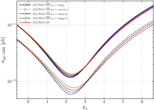
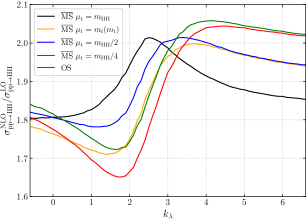
Figure 1: Left: the total inclusive cross sections at $\sqrt{s}=13.6$ TeV for different choices of the top mass renormalization scheme, at LO (dashed) and NLO (solid), as a function $\kappa_{\lambda}$. Right: the corresponding $K$-factors.

In the right panel of fig. 1, we show the $K$-factors, $K=\sigma_{NLO}/\sigma_{LO}$, as a function of the Higgs trilinear coupling for different top-mass scheme. We recall that going from a LO result to a NLO one the scheme dependence is expected to decrease. Then, schemes where the LO prediction are smaller show the largest $K$-factors.

Let us now comment on our findings for the inclusive cross as a function od $\lambda_{3}$ compared to the same study carried out with the ggHH MC code of Ref. [50] and with the results presented in Ref. [51].

The comparison with ggHH was done adopting for the top and Higgs masses and $\alpha_{s}$ the values chosen in ggHH. While we found excellent agreement within the numerical errors of the MCs for the SM, during the course of this study, we have identified a discrepancy with the existing calculation of Ref. [50] when varying $\kappa_{\lambda}$ away from its SM value. We have traced this discrepancy to the two-loop virtual contributions. We contacted the authors of ref. [50] who, using our results, found indeed an issue in their two-loop virtual contributions for values of the trilinear coupling different from the SM one. The authors of ref. [50] provided us with a fixed version of their calculation. Using these new results, we found now agreement between the two codes.

For the comparison with the results of Ref. [51] we adopted the same set of PDF employed in that work. For the SM cross section we are in agreement with the results of Ref. [51] at various center-of- mass energies including their estimate of the scale uncertainty. Instead, concerning the dependence of the cross section upon $\kappa_{\lambda}$, we find an agreement with the results of Ref. [51] at the level of per-mille for negative values of $\kappa_{\lambda}$ and for $\kappa_{\lambda}=1$. For larger positive values of $\kappa_{\lambda}$ the agreement starts to deteriorate. At the minimum of the cross section, $\kappa_{\lambda}\sim 2.4$, we find the maximal discrepancy between our and their evaluation of the inclusive cross section with a difference of several per-cent. This discrepancy is difficult to trace. On one side, the agreement with ggHH, after the fixing by the authors, and the agreement with Ref. [51] for $\kappa_{\lambda}\leq 1$ gives us confidence in our MC code. On the other side, the fact that the maximum difference is obtain at the minimum of the cross section, where the destructive interference between “signal” and “background” contributions is more pronounced, let us suspect that the way the inclusive cross section is computed in Ref. [51] from finite size bins, could be not sufficiently accurate in regions of the parameter space where there are strong cancellations. This is also suggested by the fact that we find that the discrepancy with Ref. [51] decreases for large positive value of $\kappa_{\lambda}$.

3.2 Differential Distributions

We now present the results for a selection of differential observables. As in the previous subsection we focus on the dependence of the observables upon the choice of the top-quark-mass renormalization schemes. First, we consider the SM case, $\kappa_{\lambda}=1$, then we repeat the analyis for several values of $\kappa_{\lambda}$ in order to investigate the interplay between the renormalization scheme choice and the value of the Higgs trilinear coupling.

3.2.1 Renormalization scheme dependence in the SM

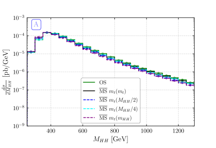
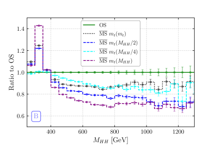
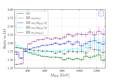
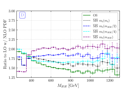
Figure 2: The invariant mass distribution of the two-Higgs system for different choices of the top-mass renormalization scheme: (A) absolute distributions at NLO+PS; (B) ratio between the $\overline{\mathrm{MS}}$ predictions and the OS one; (C) ratio between the distributions computed at NLO+PS and their LO counterpart ($K$-factors); (D) same as C but with the LO distributions computed with NLO PDFs.

In fig. 2 we show the $M_{HH}$ distribution adopting different renormalization schemes for the top mass. This and the following figures are obtained at the NLO+PS level using our Powheg MC code in conjunction with the Pythia 8 shower [71, 72]. In the top left figure, A, we present the absolute distribution that shows the peak at the opening of the $2\,m_{t}$ threshold. Although not clearly visible in the figure, the position of the peak actually depends on the top mass scheme. In fig. 2 B, the ratio between the $\overline{\mathrm{MS}}$ predictions and the OS one is shown. We notice that for large values of $M_{HH},\,(M_{HH}\geq 600$ GeV) this ratio is approximately constant with the $m_{t}(M_{HH})$ scheme giving the smallest cross section. The $\overline{\mathrm{MS}}\,m_{t}(M_{HH}/4)$ values are up to $M_{HH}\sim 700$ GeV the closest to the OS ones. In this $M_{HH}$ range the $m_{t}(M_{HH}/4)$ scheme is the one where the running of the top mass is the least. Below $M_{HH}\sim 400$ GeV the other $\overline{\mathrm{MS}}$ predictions show significant deviations from the OS one especially in the region around the opening of the $2\,m_{t}$ threshold. As already said, the opening of the $2\,m_{t}$ threshold occurs at different values of $M_{HH}$ in the various top mass schemes and therefore the ratio shown is influenced by the position of the peak. The bottom part of fig. 2 shows the $K$-factor in the various schemes. In fig. 2 C the LO result is evaluated using the LO PDF while in the NLO result the NLO PDF is used. In fig. 2 D instead, the NLO PDF is used both at LO and NLO. As already said going from a LO result to a NLO one the scheme dependence is expected to decrease. Then if an $\overline{\mathrm{MS}}$ scheme has a LO prediction smaller than the corresponding OS one its $K$-factor is expected to be larger than the OS $K$-factor and vice versa. Taking into account the information shown in fig. 2 B, one sees that the behavior of the $K$-factors in the bottom left figure shows exactly this feature. In fig. 2 D, the effects due to the variation of the PDFs are eliminated so that the pure scheme-dependent effects are more manifest. The effect induced by the variation of the PDF is quite mild as can be seen comparing figs. 2 C with 2 D.

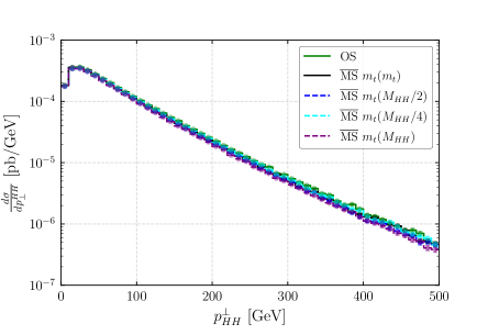
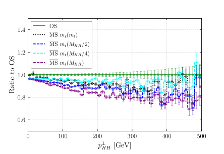
Figure 3: The transverse momentum distribution of the two-Higgs system for different choices of the top-mass renormalization scheme: (left) absolute distributions at NLO-PS; (right) ratio between the $\overline{\mathrm{MS}}$ predictions and the OS one.

The $M_{HH}$ observable is quite insensitive to shower effects. To appreciate the latter we consider two observable which are sensitive to the recoil against jet activity, namely the transverse momentum of the two Higgs system, $p^{\perp}_{HH}$, and the transverse momentum of the leading Higgs, $p^{\perp}_{H_{1}}$, that is identified as the final state boson with the largest transverse momentum.

In fig. 3 we show the transverse momentum distribution of the two Higgs system for different top mass renormalization schemes. This observable is sensitive to soft gluon radiation. In the left figure the absolute distributions at NLO+PS are presented which show the suppression in the region $p^{\perp}_{HH}\to 0$ where the fixed order NLO results become unreliable. The right plot shows the ratio between the $\overline{\mathrm{MS}}$ predictions for the $p^{\perp}_{HH}$ distribution and the OS one. We notice that the $\overline{\mathrm{MS}}$ results are always smaller than the OS one. However, in the small $p^{\perp}_{HH}$ region they are all quite close to the OS result while, as the $p^{\perp}_{HH}$ increases the $\overline{\mathrm{MS}}$ results tend to be more spread among themselves and with respect to the OS one. The small scheme dependence as $p^{\perp}_{HH}\to 0$ is likely related to the shower, that in this region has a relevant effect.

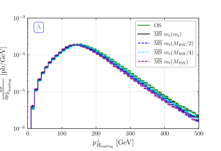
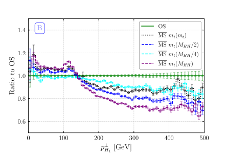
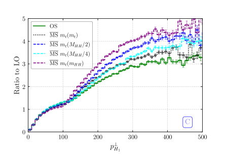
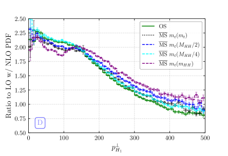
Figure 4: The transverse momentum of the leading Higgs for different choices of the top-mass renormalization scheme: (A) absolute distributions at NLO+PS; (B) ratio between the $\overline{\mathrm{MS}}$ predictions and the OS one; (C) ratio between the distributions computed at NLO+PS and their LO counterpart ($K$-factors); ( D) same as bottom left, but with the LO distributions computed with NLO PDFs.

Fig. 4 shows the same plots of fig. 2 for the transverse momentum of the leading Higgs instead of $M_{HH}$. Figs. 4 B and 4 C convey the same information with respect to the scheme dependence as the corresponding plots in fig. 2. In fig. 4 C all the $K$-factors are quite close up to $p^{\perp}_{H_{1}}\sim 100$ GeV showing that the $p^{\perp}_{H_{1}}$ predictions in this region are little scheme-dependent. For higher values of $p^{\perp}_{H_{1}}$ the scheme dependence in more pronounced and the $K$-factors can be very large. However, fig. 4 D, which is the same as plot C but with LO and NLO distributions computed with NLO PDFs, shows that the choice of the PDF plays an important role and, once the same PDF is used both at LO and NLO, the $K$-factors become smaller and the scheme dependence is approximately the same for all values of $p^{\perp}_{H_{1}}$.

3.2.2 Interplay between a modified trilinear coupling and the renormalization scheme

In this subsection the same analyses presented in the previous subsection are repeated for different values of the Higgs trilinear coupling. For shortness we concentrate on the ratio between the $\overline{\mathrm{MS}}$ predictions and the OS one at NLO+PS.

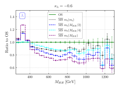
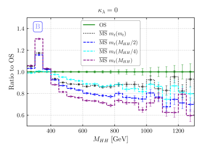
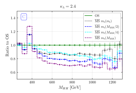
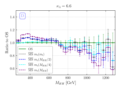
Figure 5: The invariant mass distribution of the two-Higgs system for several values of $\kappa_{\lambda}$ and different choices of the top-mass renormalization scheme: ratio between the $\overline{\mathrm{MS}}$ predictions and the OS one for $\kappa_{\lambda}=-0.6$ (A);  $\kappa_{\lambda}=0$ (B), $\kappa_{\lambda}=2.4$ (C), $\kappa_{\lambda}=6.6$ (D).

In fig. 5 the invariant mass distribution of the two Higgs system is considered. The four plots in the figure have to be compared with fig. 2 A that correponds to the case $\kappa_{\lambda}=1$. The figure shows that the cases $\kappa_{\lambda}=-0.6$ (A) and $\kappa_{\lambda}=0$ (B) are very similar to $\kappa_{\lambda}=1$. The case $\kappa_{\lambda}=0$, where there is no “signal” contribution, indicates that the scheme dependence of the “signal” part is much milder than that of the “background” one. Instead, for $\kappa_{\lambda}=2.4$ (C) i.e. the $\lambda_{3}$ value where the negative interference between the “signal” and “background” diagrams in the OS scheme is maximal, one sees that the scheme dependence is more pronounced in the region around the $2\,m_{t}$ threshold with repect to the SM case. Finally, the case $\kappa_{\lambda}=6.6$ (D) shows a much milder scheme dependence, as expected, because in this case the “signal” contribution is very amplified.

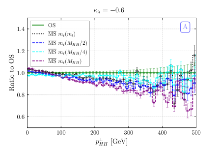
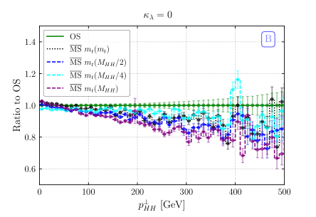
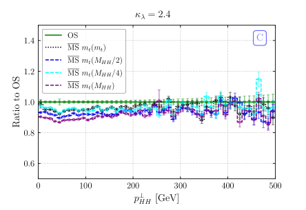
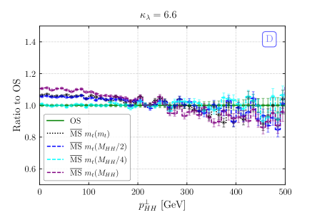
Figure 6: The transverse momentum distribution of the two-Higgs system for several values of $\kappa_{\lambda}$ and different choices of the top-mass renormalization scheme: ratio between the $\overline{\mathrm{MS}}$ predictions and the OS one for $\kappa_{\lambda}=-0.6$ (A), $\kappa_{\lambda}=0$ (B), $\kappa_{\lambda}=2.4$ (C), $\kappa_{\lambda}=6.6$ (D).

In fig. 6 we consider the transverse momentum distribution of the two Higgs system. This figure has to be compared with fig. 3 B. The cases $\kappa_{\lambda}=-0.6$ (A) and $\kappa_{\lambda}=0$ (B) are similar to the SM case although with a slightly smaller spread among the $\overline{\mathrm{MS}}$ predictions that also tend to be closer to the OS one. Instead, the cases $\kappa_{\lambda}=2.4$ (C) and $\kappa_{\lambda}=6.6$ (D) show a scheme dependence quite similar for any value of $p^{\perp}_{HH}$ and relatively small especially in the $\kappa_{\lambda}=6.6$ case.

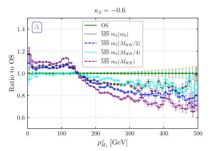
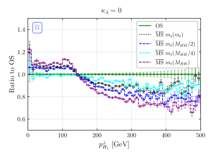
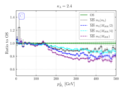
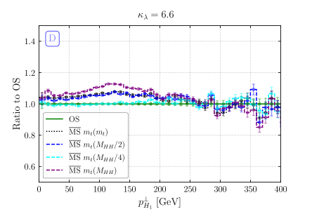
Figure 7: The transverse momentum distribution of the leading Higgs for several values of $\kappa_{\lambda}$ and different choices of the top-mass renormalization scheme: ratio between the $\overline{\mathrm{MS}}$ predictions and the OS one for $\kappa_{\lambda}=-0.6$ (A), $\kappa_{\lambda}=0$ (B), $\kappa_{\lambda}=2.4$ (C), $\kappa_{\lambda}=6.6$ (D).

Finally, fig. 7 presents the case of the transverse momentum distribution of the leading Higgs to be compared with fig. 4 B. As for the previous observables the cases $\kappa_{\lambda}=-0.6$ (A) and $\kappa_{\lambda}=0$ (B) are very similar to the SM case. The case $\kappa_{\lambda}=2.4$ (C) shows a sensible reduction of the scheme dependence in the region $p^{\perp}_{HH}\lesssim 150$ GeV, while, as before, for $\kappa_{\lambda}=6.6$ (D) the scheme dependence is very reduced.

4 Conclusions

We have presented a new MC code for Higgs boson pair production at NLO in the Powheg-Box approach. The main characteristic of this new code is the flexibility both in the inputs parameters, including the Higgs trilinear coupling, and in the choice of top-mass renormalization scheme. This is obtained employing analytic results for the two-loop virtual contributions instead of numerical grids.

Results are presented for the inclusive cross section and differential observables, including parton shower, for several values of $\lambda_{3}$ and different choices of the top mass. We find, as a general trend, that going from a LO result to a NLO one the top mass scheme dependence is reduced. However, for large invariant mass of the Higgs-pair system or large transverse momentum, the scheme dependence in the SM case, $\kappa_{\lambda}=1$, can be significant, up to $20\%$. For other values of $\kappa_{\lambda}$ we find similar results but also cases where there is a more pronounced reduction of the top mass scheme dependence.

We have compared our results with those of similar investigations present in the literature [50, 51]. We find a good agreement for the SM case with all the results present in the literature. For values of the Higgs trilinear coupling different from the SM one our results for the inclusive cross section are in agreement with those of the MC ggHH, after the authors of that code corrected their evaluation of the two-loop virtual contributions. With respect to the results of Ref.[51] we found good agreement only for $\kappa_{\lambda}\leq 1$. Given the fact that in our MC the cases $\kappa_{\lambda}\neq 1$ are obtained just assigning a value different from one to the parameter that multiplies the “signal” contribution we are quite confident in our result.

Finally we notice that our MC code is structured in such a way that can be easily extended to include other beyond the SM effects besides the rescaling of the Higgs trilinear coupling.

References

- [1] ATLAS Collaboration, G. Aad et al., “Observation of a new particle in the search for the Standard Model Higgs boson with the ATLAS detector at the LHC,” Phys. Lett. B 716 (2012) 1–29, arXiv:1207.7214 [hep-ex].
- [2] CMS Collaboration, S. Chatrchyan et al., “Observation of a New Boson at a Mass of 125 GeV with the CMS Experiment at the LHC,” Phys. Lett. B 716 (2012) 30–61, arXiv:1207.7235 [hep-ex].
- [3] ATLAS Collaboration, “Measurement of the Higgs boson mass in the decay channel using 139 fb-1 of TeV collisions recorded by the ATLAS detector at the LHC,” arXiv:2207.00320 [hep-ex].
- [4] CMS Collaboration, A. M. Sirunyan et al., “A measurement of the Higgs boson mass in the diphoton decay channel,” Phys. Lett. B 805 (2020) 135425, arXiv:2002.06398 [hep-ex].
- [5] J. Alison et al., “Higgs boson potential at colliders: Status and perspectives,” Rev. Phys. 5 (2020) 100045, arXiv:1910.00012 [hep-ph].
- [6] ATLAS Collaboration, “Constraining the Higgs boson self-coupling from single- and double-Higgs production with the ATLAS detector using collisions at TeV,” arXiv:2211.01216 [hep-ex].
- [7] CMS Collaboration, “A portrait of the Higgs boson by the CMS experiment ten years after the discovery,” Nature 607 no. 7917, (2022) 60–68, arXiv:2207.00043 [hep-ex].
- [8] G. Degrassi, P. P. Giardino, F. Maltoni, and D. Pagani, “Probing the Higgs self coupling via single Higgs production at the LHC,” JHEP 12 (2016) 080, arXiv:1607.04251 [hep-ph].
- [9] M. Gorbahn and U. Haisch, “Indirect probes of the trilinear Higgs coupling: and ,” JHEP 10 (2016) 094, arXiv:1607.03773 [hep-ph].
- [10] W. Bizon, M. Gorbahn, U. Haisch, and G. Zanderighi, “Constraints on the trilinear Higgs coupling from vector boson fusion and associated Higgs production at the LHC,” JHEP 07 (2017) 083, arXiv:1610.05771 [hep-ph].
- [11] F. Maltoni, D. Pagani, A. Shivaji, and X. Zhao, “Trilinear Higgs coupling determination via single-Higgs differential measurements at the LHC,” Eur. Phys. J. C77 no. 12, (2017) 887, arXiv:1709.08649 [hep-ph].
- [12] F. Maltoni, D. Pagani, and X. Zhao, “Constraining the Higgs self-couplings at e+ e- colliders,” JHEP 07 (2018) 087, arXiv:1802.07616 [hep-ph].
- [13] M. Gorbahn and U. Haisch, “Two-loop amplitudes for Higgs plus jet production involving a modified trilinear Higgs coupling,” JHEP 04 (2019) 062, arXiv:1902.05480 [hep-ph].
- [14] G. Degrassi and M. Vitti, “The effect of an anomalous Higgs trilinear self-coupling on the decay,” Eur. Phys. J. C 80 no. 4, (2020) 307, arXiv:1912.06429 [hep-ph].
- [15] G. Degrassi, M. Fedele, and P. P. Giardino, “Constraints on the trilinear Higgs self coupling from precision observables,” JHEP 04 (2017) 155, arXiv:1702.01737 [hep-ph].
- [16] G. D. Kribs, A. Maier, H. Rzehak, M. Spannowsky, and P. Waite, “Electroweak oblique parameters as a probe of the trilinear Higgs boson self-interaction,” Phys. Rev. D95 no. 9, (2017) 093004, arXiv:1702.07678 [hep-ph].
- [17] G. Degrassi, B. Di Micco, P. P. Giardino, and E. Rossi, “Higgs boson self-coupling constraints from single Higgs, double Higgs and Electroweak measurements,” Phys. Lett. B 817 (2021) 136307, arXiv:2102.07651 [hep-ph].
- [18] S. Di Vita, C. Grojean, G. Panico, M. Riembau, and T. Vantalon, “A global view on the Higgs self-coupling,” JHEP 09 (2017) 069, arXiv:1704.01953 [hep-ph].
- [19] L. Alasfar, J. de Blas, and R. Gröber, “Higgs probes of top quark contact interactions and their interplay with the Higgs self-coupling,” JHEP 05 (2022) 111, arXiv:2202.02333 [hep-ph].
- [20] E. W. N. Glover and J. J. van der Bij, “Higgs Boson Pair Production via Gluon Fusion,” Nucl. Phys. B309 (1988) 282–294.
- [21] D. A. Dicus, C. Kao, and S. S. D. Willenbrock, “Higgs Boson Pair Production From Gluon Fusion,” Phys. Lett. B 203 457–461.
- [22] T. Plehn, M. Spira, and P. M. Zerwas, “Pair production of neutral Higgs particles in gluon-gluon coll isions,” Nucl. Phys. B 479 (1996) 46–64, arXiv:hep-ph/9603205. [Erratum: Nucl.Phys.B 531, 655–655 (1998)].
- [23] S. Dawson, S. Dittmaier, and M. Spira, “Neutral Higgs boson pair production at hadron colliders: QCD corrections,” Phys. Rev. D58 (1998) 115012, arXiv:hep-ph/9805244 [hep-ph].
- [24] J. Grigo, J. Hoff, K. Melnikov, and M. Steinhauser, “On the Higgs boson pair production at the LHC,” Nucl. Phys. B875 (2013) 1–17, arXiv:1305.7340 [hep-ph].
- [25] J. Grigo, J. Hoff, and M. Steinhauser, “Higgs boson pair production: top quark mass effects at NLO and NNLO,” Nucl. Phys. B900 (2015) 412–430, arXiv:1508.00909 [hep-ph].
- [26] G. Degrassi, P. P. Giardino, and R. Gröber, “On the two-loop virtual QCD corrections to Higgs boson pair production in the Standard Model,” Eur. Phys. J. C76 no. 7, (2016) 411, arXiv:1603.00385 [hep-ph].
- [27] R. Frederix, S. Frixione, V. Hirschi, F. Maltoni, O. Mattelaer, P. Torrielli, E. Vryonidou, and M. Zaro, “Higgs pair production at the LHC with NLO and parton-shower effects,” Phys. Lett. B 732 (2014) 142–149, arXiv:1401.7340 [hep-ph].
- [28] F. Maltoni, E. Vryonidou, and M. Zaro, “Top-quark mass effects in double and triple Higgs production in gluon-gluon fusion at NLO,” JHEP 11 (2014) 079, arXiv:1408.6542 [hep-ph].
- [29] S. Borowka, N. Greiner, G. Heinrich, S. Jones, M. Kerner, J. Schlenk, U. Schubert, and T. Zirke, “Higgs Boson Pair Production in Gluon Fusion at Next-to-Leading Order with Full Top-Quark Mass Dependence,” Phys. Rev. Lett. 117 no. 1, (2016) 012001, arXiv:1604.06447 [hep-ph]. [Erratum: Phys. Rev. Lett.117,no.7,079901(2016)].
- [30] S. Borowka, N. Greiner, G. Heinrich, S. P. Jones, M. Kerner, J. Schlenk, and T. Zirke, “Full top quark mass dependence in Higgs boson pair production at NLO,” JHEP 10 (2016) 107, arXiv:1608.04798 [hep-ph].
- [31] J. Baglio, F. Campanario, S. Glaus, M. Mühlleitner, M. Spira, and J. Streicher, “Gluon fusion into Higgs pairs at NLO QCD and the top mass scheme,” Eur. Phys. J. C 79 no. 6, (2019) 459, arXiv:1811.05692 [hep-ph].
- [32] J. Baglio, F. Campanario, S. Glaus, M. Mühlleitner, J. Ronca, M. Spira, and J. Streicher, “Higgs-Pair Production via Gluon Fusion at Hadron Colliders: NLO QCD Corrections,” JHEP 04 (2020) 181, arXiv:2003.03227 [hep-ph].
- [33] R. Bonciani, G. Degrassi, P. P. Giardino, and R. Gröber, “Analytical Method for Next-to-Leading-Order QCD Corrections to Double-Higgs Production,” Phys. Rev. Lett. 121 no. 16, (2018) 162003, arXiv:1806.11564 [hep-ph].
- [34] J. Davies, G. Mishima, M. Steinhauser, and D. Wellmann, “Double-Higgs boson production in the high-energy limit: planar master integrals,” JHEP 03 (2018) 048, arXiv:1801.09696 [hep-ph].
- [35] J. Davies, G. Mishima, M. Steinhauser, and D. Wellmann, “Double Higgs boson production at NLO in the high-energy limit: complete analytic results,” JHEP 01 (2019) 176, arXiv:1811.05489 [hep-ph].
- [36] G. Wang, Y. Wang, X. Xu, Y. Xu, and L. L. Yang, “Efficient computation of two-loop amplitudes for Higgs boson pair production,” Phys. Rev. D 104 no. 5, (2021) L051901, arXiv:2010.15649 [hep-ph].
- [37] J. Davies, G. Heinrich, S. P. Jones, M. Kerner, G. Mishima, M. Steinhauser, and D. Wellmann, “Double Higgs boson production at NLO: combining the exact numerical result and high-energy expansion,” JHEP 11 (2019) 024, arXiv:1907.06408 [hep-ph].
- [38] L. Bellafronte, G. Degrassi, P. P. Giardino, R. Gröber, and M. Vitti, “Gluon fusion production at NLO: merging the transverse momentum and the high-energy expansions,” JHEP 07 (2022) 069, arXiv:2202.12157 [hep-ph].
- [39] G. Heinrich, S. P. Jones, M. Kerner, G. Luisoni, and E. Vryonidou, “NLO predictions for Higgs boson pair production with full top quark mass dependence matched to parton showers,” JHEP 08 (2017) 088, arXiv:1703.09252 [hep-ph].
- [40] S. Jones and S. Kuttimalai, “Parton Shower and NLO-Matching uncertainties in Higgs Boson Pair Production,” JHEP 02 (2018) 176, arXiv:1711.03319 [hep-ph].
- [41] D. de Florian and J. Mazzitelli, “Two-loop virtual corrections to Higgs pair production,” Phys. Lett. B 724 (2013) 306–309, arXiv:1305.5206 [hep-ph].
- [42] D. de Florian and J. Mazzitelli, “Higgs Boson Pair Production at Next-to-Next-to-Leading Order in QCD,” Phys. Rev. Lett. 111 (2013) 201801, arXiv:1309.6594 [hep-ph].
- [43] J. Grigo, K. Melnikov, and M. Steinhauser, “Virtual corrections to Higgs boson pair production in the large top quark mass limit,” Nucl. Phys. B 888 (2014) 17–29, arXiv:1408.2422 [hep-ph].
- [44] D. de Florian, M. Grazzini, C. Hanga, S. Kallweit, J. M. Lindert, P. Maierhöfer, J. Mazzitelli, and D. Rathlev, “Differential Higgs Boson Pair Production at Next-to-Next-to-Leading Order in QCD,” JHEP 09 (2016) 151, arXiv:1606.09519 [hep-ph].
- [45] M. Grazzini, G. Heinrich, S. Jones, S. Kallweit, M. Kerner, J. M. Lindert, and J. Mazzitelli, “Higgs boson pair production at NNLO with top quark mass effects,” JHEP 05 (2018) 059, arXiv:1803.02463 [hep-ph].
- [46] L.-B. Chen, H. T. Li, H.-S. Shao, and J. Wang, “Higgs boson pair production via gluon fusion at N3LO in QCD,” Phys. Lett. B 803 (2020) 135292, arXiv:1909.06808 [hep-ph].
- [47] L.-B. Chen, H. T. Li, H.-S. Shao, and J. Wang, “The gluon-fusion production of Higgs boson pair: N3LO QCD corrections and top-quark mass effects,” JHEP 03 (2020) 072, arXiv:1912.13001 [hep-ph].
- [48] S. Frixione, P. Nason, and C. Oleari, “Matching NLO QCD computations with Parton Shower simulations: the POWHEG method,” JHEP 11 (2007) 070, arXiv:0709.2092 [hep-ph].
- [49] S. Alioli, P. Nason, C. Oleari, and E. Re, “A general framework for implementing NLO calculations in shower Monte Carlo programs: the POWHEG BOX,” JHEP 06 (2010) 043, arXiv:1002.2581 [hep-ph].
- [50] G. Heinrich, S. P. Jones, M. Kerner, G. Luisoni, and L. Scyboz, “Probing the trilinear Higgs boson coupling in di-Higgs production at NLO QCD including parton shower effects,” JHEP 06 (2019) 066, arXiv:1903.08137 [hep-ph].
- [51] J. Baglio, F. Campanario, S. Glaus, M. Mühlleitner, J. Ronca, and M. Spira, “ : Combined uncertainties,” Phys. Rev. D 103 no. 5, (2021) 056002, arXiv:2008.11626 [hep-ph].
- [52] G. Passarino and M. J. G. Veltman, “One Loop Corrections for Annihilation Into in the Weinberg Model,” Nucl. Phys. B 160 (1979) 151–207.
- [53] A. Denner, S. Dittmaier, and L. Hofer, “COLLIER - A fortran-library for one-loop integrals,” PoS LL2014 (2014) 071, arXiv:1407.0087 [hep-ph].
- [54] U. Aglietti, R. Bonciani, G. Degrassi, and A. Vicini, “Analytic Results for Virtual QCD Corrections to Higgs Production and Decay,” JHEP 01 (2007) 021, arXiv:hep-ph/0611266 [hep-ph].
- [55] C. Anastasiou, S. Beerli, S. Bucherer, A. Daleo, and Z. Kunszt, “Two-loop amplitudes and master integrals for the production of a Higgs boson via a massive quark and a scalar-quark loop,” JHEP 01 (2007) 082, arXiv:hep-ph/0611236 [hep-ph].
- [56] R. N. Lee, “LiteRed 1.4: a powerful tool for reduction of multiloop integrals,” J. Phys. Conf. Ser. 523 (2014) 012059, arXiv:1310.1145 [hep-ph].
- [57] R. N. Lee, “Presenting LiteRed: a tool for the Loop InTEgrals REDuction,” arXiv:1212.2685 [hep-ph].
- [58] A. von Manteuffel and L. Tancredi, “A non-planar two-loop three-point function beyond multiple polylogarithms,” JHEP 06 (2017) 127, arXiv:1701.05905 [hep-ph].
- [59] https://github.com/mppmu/hhgrid.
- [60] L. Naterop, A. Signer, and Y. Ulrich, “handyG —Rapid numerical evaluation of generalised polylogarithms in Fortran,” Comput. Phys. Commun. 253 (2020) 107165, arXiv:1909.01656 [hep-ph].
- [61] R. Bonciani, G. Degrassi, P. P. Giardino, and R. Gröber, “A Numerical Routine for the Crossed Vertex Diagram with a Massive-Particle Loop,” Comput. Phys. Commun. 241 (2019) 122–131, arXiv:1812.02698 [hep-ph].
- [62] K. Melnikov and T. v. Ritbergen, “The Three loop relation between the MS-bar and the pole quark masses,” Phys. Lett. B 482 (2000) 99–108, arXiv:hep-ph/9912391.
- [63] M. Carena, D. Garcia, U. Nierste, and C. E. M. Wagner, “Effective Lagrangian for the interaction in the MSSM and charged Higgs phenomenology,” Nucl. Phys. B 577 (2000) 88–120, arXiv:hep-ph/9912516.
- [64] V. Hirschi, R. Frederix, S. Frixione, M. V. Garzelli, F. Maltoni, and R. Pittau, “Automation of one-loop QCD corrections,” JHEP 05 (2011) 044, arXiv:1103.0621 [hep-ph].
- [65] E. Bagnaschi and A. Vicini, “The Higgs transverse momentum distribution in gluon fusion as a multiscale problem,” JHEP 01 (2016) 056, arXiv:1505.00735 [hep-ph].
- [66] E. Bagnaschi, R. V. Harlander, H. Mantler, A. Vicini, and M. Wiesemann, “Resummation ambiguities in the Higgs transverse-momentum spectrum in the Standard Model and beyond,” JHEP 01 (2016) 090, arXiv:1510.08850 [hep-ph].
- [67] L. Alasfar et al., “Effective Field Theory descriptions of Higgs boson pair production,” arXiv:2304.01968 [hep-ph].
- [68] GoSam Collaboration, G. Cullen et al., “GS-2.0: a tool for automated one-loop calculations within the Standard Model and beyond,” Eur. Phys. J. C 74 no. 8, (2014) 3001, arXiv:1404.7096 [hep-ph].
- [69] GoSam Collaboration, G. Cullen, N. Greiner, G. Heinrich, G. Luisoni, P. Mastrolia, G. Ossola, T. Reiter, and F. Tramontano, “Automated One-Loop Calculations with GoSam,” Eur. Phys. J. C 72 (2012) 1889, arXiv:1111.2034 [hep-ph].
- [70] NNPDF Collaboration, R. D. Ball et al., “Parton distributions from high-precision collider data,” Eur. Phys. J. C 77 no. 10, (2017) 663, arXiv:1706.00428 [hep-ph].
- [71] T. Sjostrand, S. Mrenna, and P. Z. Skands, “A Brief Introduction to PYTHIA 8.1,” Comput. Phys. Commun. 178 (2008) 852–867, arXiv:0710.3820 [hep-ph].
- [72] T. Sjöstrand, S. Ask, J. R. Christiansen, R. Corke, N. Desai, P. Ilten, S. Mrenna, S. Prestel, C. O. Rasmussen, and P. Z. Skands, “An introduction to PYTHIA 8.2,” Comput. Phys. Commun. 191 (2015) 159–177, arXiv:1410.3012 [hep-ph].