Polynomial-time Solver of Tridiagonal QUBO and QUDO problems with Tensor Networks

Abstract

We present an algorithm for solving tridiagonal Quadratic Unconstrained Binary Optimization (QUBO) problems and Quadratic Unconstrained Discrete Optimization (QUDO) problems with one-neighbor interactions using the quantum-inspired technology of tensor networks. Our method is based on the simulation of a quantum state to which we will apply an imaginary time evolution and perform a series of partial traces to obtain the state of maximum amplitude, since it will be the optimal state. We will also deal with the degenerate case and check the polynomial complexity of the algorithm.

1 Introduction

Quadratic Unconstrained Binary Optimization (QUBO) [1] problems are a type of combinatorial optimization problem that lies at the intersection of quantum computing and optimization theory. These problems are characterized by their ability to represent a wide variety of complex challenges and their use in industrial and applied fields such as logistics [2] [3], engineering [4], physics, biology [5] and economics [6].

In a QUBO problem, one seeks to find an assignment of binary values (0 or 1) to a set of decision variables such that a quadratic function of these variables is minimized. This quadratic function, also known as a cost or energy function, can represent constraints and objectives of a specific problem. Quadratic Unconstrained Discrete Optimization (QUDO) problems are a generalization of the QUBO problems, allowing the variables to take a larger number of integer values.

These QUBO and QUDO problems have a degree of complexity too high to be solved classically in an efficient way [7], so they are usually solved with approximate or heuristic methods, such as genetic algorithms [8]. QUBO problems are particularly interesting and relevant in the era of quantum computing for their ability to take advantage of the properties of quantum computing.

However, due to the current state of quantum hardware and its availability, the field of quantum-inspired technologies, which consist of simulating certain quantum properties and taking advantage of them to accelerate calculations, has gained importance. One of the most important are tensor networks [9], which use the algebraic mathematics of quantum systems to simulate them classically and extract certain properties of the simulated systems, being able to implement operations that would not be possible in quantum systems, such as forced post-selection or the application of non-unitary operators.

In this paper we will explore how to solve with tensor networks general QUBO and QUDO problems with one-neighbor interactions in an efficient way by means of a sequential tensor network contraction algorithm that simulates an imaginary time evolution and a partial trace. We will also analyze its applicability to degenerate cases and see its computational complexity.

2 Description of the problem

A general QUBO problem can be expressed by a quadratic cost function to be minimized by a vector of $N$ binary components of a vector $\vec{x}$. That is, we look for an optimal $\vec{x}_{\text{opt}}$ such that

$$\vec{x}_{\text{opt}}= \arg\min_{\vec{x}}C(\vec{x})$$ (1)

$$C(\vec{x})= \sum_{\begin{subarray}{c}i,j=0\\ i\leq j\end{subarray}}^{N-1}w_{ij}x_{i}x_{j},\qquad x_{i}\in\{0,1\},$$ (2)

where $w_{ij}$ are the elements of the weight matrix $w$ of the problem. The diagonal elements $w_{ii}$ are the local terms and the the non-diagonal elements $w_{ij}$ are the interaction terms.

In a QUDO case, the problem is analogous, changing that the components of $\vec{x}$ will be integers in a certain range, not only $0$ or $1$. This is

$$\vec{x}_{\text{opt}}= \arg\min_{\vec{x}}C(\vec{x})$$ (3)

$$C(\vec{x})= \sum_{\begin{subarray}{c}i,j=0\\ i\leq j\end{subarray}}^{N-1}w_{i,j,x_{i},x_{j}}$$ (4)

$$x_{i}\in \{0,1,\dots,D_{i}-1\},$$

where $w_{i,j,x_{i},x_{j}}$ are the elements of the weight tensor $w$ of the problem, which depends on the state of the variables and its positions in the solution, and $D_{i}$ are the number of possible values of the variable $x_{i}$.

A special case of interest is the case of nearest neighbor interaction in a linear chain, which can be understood as the Ising model in one dimension. In this problem, each variable interacts only with the one it has before and with the one it has just after. Therefore, our QUBO problem simplifies to

$$\vec{x}_{\text{opt}}= \arg\min_{\vec{x}}C(\vec{x})$$ (5)

$$C(\vec{x})= \sum_{i=0}^{N-1}w_{i,i}x_{i}+\sum_{i=0}^{N-2}w_{i,i+1}x_{i}x_{i+1},\quad x_{i}\in\{0,1\},$$ (6)

which implies that $w$ is a tridiagonal matrix.

In the QUDO case, the analogous problem would be

$$\vec{x}_{\text{opt}}= \arg\min_{\vec{x}}C(\vec{x})$$ (7)

$$C(\vec{x})= \sum_{i=0}^{N-1}w_{i,i,x_{i},x_{i}}+\sum_{i=0}^{N-2}w_{i,i+1,x_{i},x_{i+1}}$$ (8)

$$x_{i}\in \{0,1,\dots,D_{i}-1\},$$

which could be considered a kind of generalized travelling salesman without restrictions, where the distances change every time.

3 Tridiagonal QUBO tensor network solver

First we will create a solver for the tridiagonal QUBO problem and then we will see how to generalize it to the QUDO problem. We use a modified version of the method [10].

For this, we will use the tensor network of Fig. 1 a, where the ‘+’ nodes are nodes representing a qubit in uniform superposition $(1,1)$ and the $T$ nodes represent the imaginary time evolution that depends on the state of the two neighboring qubits.

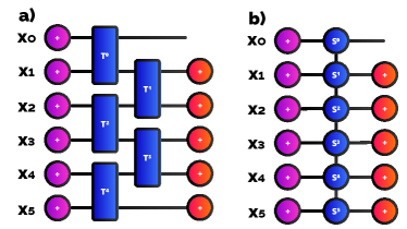
Figure 1: Tensor networks solving the tridiagonal QUBO problem and the one-neighbor QUDO problem. a) Bilocal version, b) Matrix Product Operator (MPO) version.

The ‘+’ nodes are a representation of the state of each variable $x_{i}$. It can be visualized as the initialization of a quantum circuit. By performing the tensor product with all these tensors, each one being in uniform superposition, we will have the uniform superposition of all $2^{N}$ combinations.

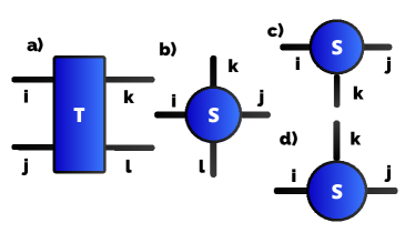
Figure 2: Tensor indexes. a) $T$ tensor, b) First $S$ tensor, c) Intermediate $S$ tensor, d) Final $S$ tensor.

The $T$ tensors will be tensors with 4 2-dimensional indexes $i,j,k,l$ (Fig. 2) whose non-zero elements will be those in which $i=k$ and $j=l$, so that the state of qubit 1 enters at index $i$ and exits at index $k$ and the state of qubit 2 enters at index $j$ and exits at index $l$. The non-zero elements will be

$$T^{n}_{ijkl}=\begin{cases}1&\text{ if }i=0\ \forall j\\ e^{-\tau w_{n,n}}&\text{ if }i=1,j=0\\ e^{-\tau\Omega_{n}}&\text{ if }i=1,j=1\end{cases}$$ (9)

$$T^{N-2}_{ijkl}=\begin{cases}1&\text{ if }i,j=0,0\\ e^{-\tau w_{N-2,N-2}}&\text{ if }i,j=1,0\\ e^{-\tau w_{N-1,N-1}}&\text{ if }i,j=0,1\\ e^{-\tau\left(\Omega_{N-2,N-2}+w_{N-1,N-1}\right)}&\text{ if }i,j=1,1\end{cases}$$ (10)

where $\Omega_{n}=w_{n,n}+w_{n,n+1}$, $\tau$ is a decay hyperparameter and $T^{n}$ is the $T$-tensor which connects the variables $n$ and $n+1$.

The goal is for our tensor layer $T$ to make the state encoded in our tensor network to be

$$|\psi\rangle=\sum_{\vec{x}}e^{-\tau C(\vec{x})}|\vec{x}\rangle,$$ (11)

so that the combination with the lowest cost has an exponentially larger amplitude than the other combinations.

However, because this state will be a tensor of $2^{N}$ components, we cannot simply look at which component has the largest amplitude, so we will extract its information in a more efficient way.

Let us assume that the amplitude of the lowest cost combination is sufficiently larger than the other amplitudes of the other combinations. This is a reasonable assumption, because if we increase $\tau$, the combinations will change their amplitudes in exponentially different ways.

If there is a combination with a sufficiently higher amplitude, if we add up all the combinations with $x_{0}=0$ and all the combinations with $x_{0}=1$ separately, the main contribution will be that of the combination with a higher amplitude. We will call this operation partial trace with $x_{0}$ free, which returns a vector $P^{x_{0}}$ with components

$$P^{x_{0}}_{i}=\sum_{\begin{subarray}{c}\vec{x}\\ x_{0}=i\end{subarray}}e^{-\tau C(\vec{x})}.$$ (12)

In this case, if the combination with the largest amplitude has $x_{0}=0$, then $P^{x_{0}}_{0}>P^{x_{0}}_{1}$, and in the opposite case, $P^{x_{0}}_{0}<P^{x_{0}}_{1}$.

This is done by connecting a ‘+’ tensor into each of the qubits at the output of the $T$ tensor layer, except for the $x_{0}$ qubit.

We can optimize the contraction of the tensor network by defining it as shown in Fig. 1 b, where we replace the $T$-tensors by a Matrix Product Operator (MPO) layer of $S$-tensors that performs exactly the same function, sending signals up and down through its bound indexes $k,l$. All its indexes will be of dimension 2. These will tell the adjacent $S$ tensor what the state of its associated qubit is and, depending on the signal they receive from the previous $S$ tensor and their own qubit, apply a certain evolution in imaginary time. This tensor network is much easier and more straightforward to contract. We will call $S^{n}$ the $S$-tensor connected with the variable $x^{n}$.

Therefore, the non-zero elements of the $S$-tensors will be those where $i=j$ for $S^{0}$ and $S^{N-1}$, and $i=j=l$ for the others. Their values will be

$$S^{0}_{ijk}=\begin{cases}1&\text{ if }i,k=0,0\\ e^{-\tau w_{0,0}}&\text{ if }i,k=1,1\end{cases}$$ (13)

$$S^{n}_{ijkl}=\begin{cases}1&\text{ if }i=0\ \forall k\\ e^{-\tau w_{n,n}}&\text{ if }i,k=1,0\\ e^{-\tau\Theta_{n}}&\text{ if }i,k=1,1,\end{cases}$$ (14)

$$S^{N-1}_{ijk}=\begin{cases}1&\text{ if }i=0\ \forall k\\ e^{-\tau w_{N-1,N-1}}&\text{ if }i,k=1,0,\\ e^{-\tau\Theta_{N-1}}&\text{ if }i,k=1,1,\end{cases}$$ (15)

being $\Theta_{n}=w_{n,n}+w_{n-1,n}$.

With this method we can determine the variable $x_{0}$, and to determine the other components we will follow the following steps:

1. Perform the algorithm for the $x_{0}$ component.

2. For $n\in[1,N-2]$:

   • Carry out the same algorithm, but eliminating the previous $n-1$ variables and changing the new tensor $S^{0}$ so that its components are the same as those of the tensor $S^{1}$ from the previous step with its index $k$ set to $x_{n-1}$. This means

     $$S^{0}_{ijk}=S^{1,\text{previous}}_{i,j,x_{n-1},l}.$$ (16)

     The result of the algorithm will be $x_{n}$.

3. For $x_{N-1}$, we use classical comparison:

   • If $x_{N-2}=0$:

     • $x_{N-1}=1$ if $w_{N-1,N-1}<0$

     • $x_{N-1}=0$ if $w_{N-1,N-1}>0$.

   • If $x_{N-2}=1$:

     • $x_{N-1}=1$ if $\Theta_{N-1}<0$

     • $x_{N-1}=0$ if $\Theta_{N-1}>0$.

The progressive reduction of the represented qubits is due to the fact that, if we already know the solution, we can consider the rest of the unknown system and introduce the known information to the system. The redefinition of the tensor $S^{0}$ at each step allows us to take into consideration the result of the previous step in obtaining the costs of what would be the pair of the variable to be determined and the previous one.

4 One-neighbor QUDO problem

In this case we are going to solve the one-neighbor QUDO problem making use of the tridiagonal QUBO algorithm in an extended version. Here we will only have to change our qubit formalism to a qudit formalism and allow the indexes of the tensor network in Fig. 1 to have the dimension that is required in each variable. From here on, the variable $x_{i}$ will have $D_{i}$ possible values.

The ‘+’ tensors will now each have $D_{i}$ components, depending on the variable they represent. The same for those we use to make the partial trace. The indexes of the $S$ tensors will have the following dimensions:

• $S^{0}$: $i,j,k$ dimension $D_{0}$.

• $S^{n}$: $i,j,l$ dimension $D_{n}$. $k$ dimension $D_{n-1}$.

• $S^{N-1}$: $i,j$ dimension $D_{N-1}$. $k$ dimension $D_{N-2}$.

Once again, the elements of the $S$-tensors are non-zero when $i=j$ for $S^{0}$ and $S^{N-1}$, and $i=j=l$ for the others. They are

$$S^{0}_{ijk}=e^{-\tau w_{0,0,i,i}}\text{ if }i=k$$ (17)

$$S^{n}_{ijkl}=e^{-\tau\left(w_{n,n,i,i}+w_{n-1,n,i,k}\right)}$$ (18)

$$S^{N-1}_{ijk}=e^{-\tau\left(w_{N-1,N-1,i,i}+w_{N-2,N-1,k,i}\right)}.$$ (19)

As in the QUBO case, the $S$-tensors receive the state of the adjacent qudit through the index $k$ and send theirs through the index $l$.

If we contract this tensor network analogously to the QUBO case, we obtain a vector $P^{x_{0}}$ of dimension $D_{0}$. From this we can extract the optimal value of $x_{0}$ by seeing which component has the largest value. That is, if the vector obtained by the tensor network were $(2,4,27,2,0,1)$, the correct value for $x_{0}$ will be $2$.

To obtain the other variables, we will perform exactly the same process that we have explained for the QUBO case, changing the last step to a comparison that gives us the $x_{N-1}$ that will give us a lower cost based on the $x_{N-2}$ we already have.

5 Tracing optimization

One of the biggest problems we may encounter is to choose a value of $\tau$ large enough to distinguish the combinations but not so large that the amplitudes go to zero. For this reason, in practice it is advisable to rescale the $w$ matrix before starting so that the scale of the minimum costs does not vary too much from one problem to the next and we can leave $\tau$ constant.

To deal with this, an effective way to modify the general algorithm is to initialize in a superposition with complex phases between the base combinations instead of initializing with a superposition with the same phase. This allows us that, at the time of partial tracing, instead of summing all amplitudes in the same direction, they will be summed as 2-dimensional vectors. This allows the sub-optimal states to be damped against each other allowing the maximum to be seen better.

We will add these phases by making the initialization ‘+’ tensors instead of being $(1,1,\dots,1)$, they will be $(e^{2\pi i\cdot 0\frac{1}{D_{n}}},e^{2\pi i\cdot 1\frac{1}{D_{n}}},e^{2\pi i\cdot 2\frac{1}{D_{n}}},\dots,e^{2\pi i\cdot(D_{n}-1)\frac{1}{D_{n}}})$. Thus, each base state has its own associated phase. To improve performance, we can add a small random factor to each state phase.

In this case we only need to change the definition of $P^{x_{0}}$ to

$$P^{x_{0}}_{i}=\left|\left|\sum_{\begin{subarray}{c}\vec{x}\\ x_{0}=i\end{subarray}}e^{i\gamma_{\vec{x}}}e^{-\tau C(\vec{x})}\right|\right|,$$ (20)

being $\gamma_{\vec{x}}$ the phase of the $\vec{x}$ state.

6 Degenerate case

So far we have considered a non-degenerate case. However, in the degenerate case where we have more than one optimal combination, we have two peaks of exactly equal amplitude. In the phased method we can have the situation where the two peaks have opposite phase, so that they cancel out and we cannot see the optimum. For this reason, we recommend that the phased version should not be used in case of a possible degeneration of the problem.

Our method without phases allows us to avoid the degeneracy problem, because, if in any step of the process we have the two peaks in two different $x_{n}$ values, we will choose one of them and the rest of the combination we obtain will be the one associated exactly to the $x_{n}$ we have chosen, so we avoid the degeneracy problem. In addition, if we want the other states of the degeneracy, we can do the same thing again, but choosing the other high amplitude component instead.

7 Complexity analysis

Before analyzing the computational complexity, we have to emphasize that the tensor network can be further optimized if we take into account the fact that the contraction of the ‘+’ tensors with the $S$ tensors only implies that the resulting tensors will be the same as the $S$ tensors that created them, but simply eliminating the $i$ index, so the optimal tensor network would be exactly the same as in Fig. 1 b, but eliminating the first layer of ‘+’ tensors and their associated indexes in the $S$ tensors. This tensor network is the one in Fig. 3 a.

The complexity of contracting each of the tensor networks for a QUDO problem with $N$ variables that can take $D$ values is $O(ND^{3})$. This is due to we have to apply the contraction scheme in Fig. 3. We have to repeat it $N-1$ times, so the total algorithm complexity is $O(N^{2}D^{3})$. In the QUBO case, the complexity is $O(N^{2}2^{3})$.

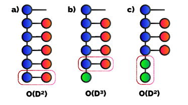
Figure 3: Contraction scheme for the efficient tensor network. We have to repeat this process $N-1$ times to obtain a component. a) Partial trace of the last variable. b) Partial trace of the penultimate variable. c) Contraction of the last variable with the penultimate one.

8 Conclusions

We have developed a method in tensor networks that allows us to efficiently solve tridiagonal QUBO problems and one-neighbor QUDO problems in an efficient way. We have also seen how they can perform in degenerate cases and what is their computational complexity. Next lines of research will be to obtain a method to determine the $\tau$ for each problem, for example, with the idea we proposed in [11]. Another possible line will be the efficient resolution of more general QUBO and QUDO problems with this methodology and its application to various industrial problems.

References

-
[1]
Fred Glover, Gary Kochenberger, Yu Du.
A Tutorial on Formulating and Using QUBO Models,
arXiv:1811.11538 [cs.DS], (2019). -
[2]
Juan Francisco Ariño Sales, Raúl Andres Palacios Araos.
Adiabatic Quantum Computing for Logistic Transport Optimization,
arXiv:2301.07691 [quant-ph], (2023). -
[3]
Sebastián V. Romero, Eneko Osaba, Esther Villar-Rodriguez, Antón Asla.
Solving Logistic-Oriented Bin Packing Problems Through a Hybrid Quantum-Classical Approach,
arXiv:2308.02787 [cs.AI], (2023). -
[4]
Matsumori, T., Taki, M. & Kadowaki, T.
Application of QUBO solver using black-box optimization to structural design for resonance avoidance.
Sci Rep 12, 12143 (2022). https://doi.org/10.1038/s41598-022-16149-8 -
[5]
T. Zaborniak, J. Giraldo, H. Müller, H. Jabbari and U. Stege,
"A QUBO model of the RNA folding problem optimized by variational hybrid quantum annealing",
2022 IEEE International Conference on Quantum Computing and Engineering (QCE), Broomfield, CO, USA, 2022, pp. 174-185, doi: 10.1109/QCE53715.2022.00037 -
[6]
Mirko Mattesi, Luca Asproni, Christian Mattia, Simone Tufano, Giacomo Ranieri, Davide Caputo, Davide Corbelletto.
Financial Portfolio Optimization: a QUBO Formulation for Sharpe Ratio Maximization.
arXiv:2302.12291 [quant-ph], (2023). -
[7]
Hirotoshi Yasuoka.
Computational Complexity of Quadratic Unconstrained Binary Optimization,
arXiv:2109.10048 [cs.CC], (2022). -
[8]
Koji Nakano, Daisuke Takafuji, Yasuaki Ito, Takashi Yazane, Junko Yano, Shiro Ozaki, Ryota Katsuki, Rie Mori.
Diverse Adaptive Bulk Search: a Framework for Solving QUBO Problems on Multiple GPUs,
arXiv:2207.03069 [cs.PF], (2023). -
[9]
Jacob Biamonte, Ville Bergholm.
Tensor Networks in a Nutshell.
arXiv:1708.00006 [quant-ph], (2017). -
[10]
Hao Tianyi, Huang Xuxin, Jia Chunjing, Peng Cheng.
A Quantum-Inspired Tensor Network Algorithm for Constrained Combinatorial Optimization Problems. Frontiers in Physics, Vol 10
10.3389/fphy.2022.906590, (2022). -
[11]
Alejandro Mata Ali, Iñigo Perez Delgado, Marina Ristol Roura, Aitor Moreno Fdez. de Leceta.
Efficient Finite Initialization for Tensorized Neural Networks,
arXiv:2309.06577 [cs.LG], (2023).