Learning End-to-End Channel Coding with Diffusion Models

Abstract

The training of neural encoders via deep learning necessitates a differentiable channel model due to the backpropagation algorithm. This requirement can be sidestepped by approximating either the channel distribution or its gradient through pilot signals in real-world scenarios. The initial approach draws upon the latest advancements in image generation, utilizing generative adversarial networks (GANs) or their enhanced variants to generate channel distributions. In this paper, we address this channel approximation challenge with diffusion models, which have demonstrated high sample quality in image generation. We offer an end-to-end channel coding framework underpinned by diffusion models and propose an efficient training algorithm. Our simulations with various channel models establish that our diffusion models learn the channel distribution accurately, thereby achieving near-optimal end-to-end symbol error rates (SERs). We also note a significant advantage of diffusion models: A robust generalization capability in high signal-to-noise ratio regions, in contrast to GAN variants that suffer from error floor. Furthermore, we examine the trade-off between sample quality and sampling speed, when an accelerated sampling algorithm is deployed, and investigate the effect of the noise scheduling on this trade-off. With an apt choice of noise scheduling, sampling time can be significantly reduced with a minor increase in SER.

I Introduction

I-A DL-Based End-to-End Channel Coding

In traditional communication systems, optimal transmission rates for reliable communication necessitate meticulous adaption of practical codes, i.e., encoders and decoders, tailored to specific channel configurations. This requirement can be particularly challenging in dynamic environments, underscoring the need for a more automated approach, particularly in the context of non-standard channel models.

To address this requirement, numerous studies have proposed the use of deep learning (DL) for the optimization of not only encoders and decoders but also modulators and demodulators. This approach was pursued independently until [2, 3] proposed an end-to-end (E2E) framework for the joint optimization of these elements. This E2E framework, closely resembling the autoencoder (AE) model with a wireless channel block inserted between the encoder and decoder blocks [2], integrates a modulator within the encoder component. This arrangement allows for spreading and adding redundancy to the encoded and modulated symbols to combat channel noise, as opposed to the traditional AE function of input compression. Correspondingly, the decoder and demodulator are combined into a single neural network (NN) model.

The performance of AE-based E2E communication frameworks has been proven to be robust, providing error probability performance comparable to or better than that of classical channel coding methods in various cases [4, 5]. For gradient-based optimization of the encoder, the channel between the encoder and decoder should be known and differentiable to apply the backpropagation algorithm. However, the differentiability of channels is often not ensured as they can be too complex to be accurately depicted by straightforward mathematical models, or in some cases, we may not have a channel model, but only be able to sample from it.

To circumvent this issue, there are two principal strategies: the generation of the channel output distribution by a generative model [6, 7, 8, 9], and the approximation of the channel gradient by perturbing the channel probing variable and comparing the change in rewards, which is referred to as reinforcement learning (RL) and a corresponding policy gradient method [10]. This paper employs the generative models approach, given its applicability not only for E2E channel coding optimization but also for learning stochastic channel models [11, 12], and channel estimation [13, 14, 15, 16, 17, 18] under certain channel model assumptions.

This study aims to examine the potential for learning channel distributions using diffusion, a powerful generative method, as an alternative to the commonly used generative adversarial networks (GANs) [8, 6], and their variations such as the Wasserstein GAN (WGAN) [7], and the residual-aided-GAN (RA-GAN) [9]. While GAN-based models have demonstrated their capabilities for producing high-quality samples with a fast sampling speed, they often suffer from mode collapse, a problem associated with generating only the most probable samples and failing to cover the entire sample distribution [19]. Conversely, diffusion models can generate high-quality samples with good mode coverage, albeit at the cost of extended sampling times compared to GANs [19]. Therefore, diffusion models could be advantageous in scenarios where learning complex channel distributions is the primary objective, assuming sufficient computational power is available to offset the slow sampling speed.

Diffusion models generate data samples by adding noise until the samples follow a normal distribution, and they learn to denoise the noisy samples to reconstruct the original data samples. By applying the denoising procedure to noise samples from the normal distribution, new samples can be generated. While diffusion models might take several forms, there exist three principal variants characterized by unique methodologies for perturbing training samples and learning to denoise them [20]. These include diffusion-denoising probabilistic model (DDPM) [21, 22], noise-conditioned score networks (NNCNs) [23], and models based on stochastic differential equations (SDEs) [24]. This study uses a DDPM to generate a channel distribution, a decision motivated by a substantial body of research utilizing DDPMs for conditional generation. Typically, channels are defined by a conditional distribution, making DDPMs an apt choice for our purpose.

I-B Related Works: E2E Learning with Generated Channel

Several studies that closely align with our work have explored E2E communication by learning channel distributions using a generative model. This approach was first evaluated in [6], where a conditional GAN was evaluated using the symbol error rate (SER) of the entire framework for an additive white Gaussian noise (AWGN) channel and a Rayleigh fading channel. Comparisons were made to traditional encoding and modulation methods, as well as to an AE trained with the channels with coherent detection. The SER performance was found to be comparable to that of traditional methods for these channel models, although the generated channel exhibited a noticeable performance gap compared to the framework with coherent detection.

This approach later saw advancements with the work presented in [7], where a Wasserstein GAN (WGAN) was utilized for robust channel estimation performance for an over-the-air channel. Their results, assessed by the channel impulse response, demonstrated a bit error rate (BER) comparable to an RL-based framework for an AWGN channel. An RA-GAN [9] was subsequently introduced to stabilize the training process, exhibiting near-optimal SER performance and lower training time compared to the WGAN. While the RA-GAN performed well without issues of mode collapse on various channel models, the WGAN encountered mode collapse when trained for highly variable and dynamic channels.

This has spurred the communication research community to explore more robust generative neural networks that circumvent the challenges often seen with GANs in computer vision. These new approaches include normalizing flows [17], score-based generative model [14] and variational AE [12]. These studies primarily focus on channel estimation and have not provided the E2E communication performance. To the best of our knowledge, no study has yet utilized diffusion models for channel estimation or for E2E learning of a communication framework. In this paper, we introduce diffusion models for channel generation and evaluate their performance for an AWGN channel, a Rayleigh fading channel, and a solid state high-power amplifier (SSPA) channel. This evaluation involves comparisons to WGANs and the optimal case with a known channel model. Our specific contributions will be detailed in the following subsection.

I-C Main Contributions

Image generation and channel approximation represent two distinct application areas, with the optimal solution in one not necessarily translating to superior performance in the other. The primary objective of this paper is to construct a diffusion model for channel approximation with the aim of enhancing several key performance parameters. These include E2E error probability, the convergence NNs in the framework, and sampling speed. The specific contributions are as follows:

• We present an E2E NN-based channel coding framework that incorporates a diffusion model. This design is capable of even handling channels that are unknown or non-differentiable.

• We propose an efficient pre-training algorithm for the E2E framework. Our method not only achieves faster and more stable convergence but also results in smaller E2E error probabilities compared to the commonly used iterative training algorithm. However, it is noteworthy that our approach requires a larger model complexity in our experiment.

• We optimized the design of the diffusion models, achieving near-optimal E2E error probabilities in simulations. It was observed that the diffusion model provides stronger generalization performance in high-SNR regions, in contrast to GANs that display an error floor in such regions.

• We implemented state-of-the-art schemes from computer vision to improve the sample quality and sampling time of the diffusion model. This includes the application of corrected noise scheduling [25], an improved parameterization [26], and the skipped sampling algorithm of denoising diffusion implicit models (DDIMs) [27]. We provide an analysis of their effectiveness in the E2E communication context. Additionally, we experimentally explored a noise scheduling method that offers a favorable trade-off between sample quality and sampling time.

I-D Notation

A stochastic process $x_{1},x_{2},\dots,x_{t}$ indexed by time step $t$ can be shortened as $x_{1:t}$. An $n$-dimensional random vector is represented as $X^{n}$, and $X_{i}$ refers to its $i^{\text{th}}$ element for $i=1,2,\dots,n$. The $n$-dimensional identity matrix is denoted by $I_{n}$. The $\ell_{2}$-norm of a vector $x$ is denoted by $||x||_{2}$. When a probability distribution, a function, a scalar, a vector, and a matrix have the subscript $\theta$, that means they are learned by NNs. In this paper, $\mathcal{U}\{a,b\}$ indicates the discrete uniform distribution over the integers in $[a,b]$ for arbitrary integers $a,b$ such that $a<b$. When we refer to the distribution that a normal random variable $X$ follows, the notation $X\sim\mathcal{N}(\mu,\sigma^{2})$ is used for $\mu\in\mathbb{R}$ and $\sigma>0$. When the probability distribution $p(X)$ of a random variable $X$ is referred to, we use the notation $p(X)=\mathcal{N}(X;\mu,\sigma^{2})$, where the variable and parameters are separated by a semicolon.

II Diffusion Models

A diffusion model consists of a forward and a reverse diffusion process. Given an input sample from some data distribution $x_{0}\sim q(x)$, a forward diffusion process can be defined, which progressively adds Gaussian noise to the sample over $T$ time steps, producing increasingly noisy samples $x_{1},\ldots,x_{T}$ of the original sample. This process is defined as

$$q(x_{1:T}|x_{0}) =\prod_{t=1}^{T}q(x_{t}|x_{t-1})$$ (1)

$$q(x_{t}|x_{t-1}) =\mathcal{N}(x_{t};\sqrt{1-\beta_{t}}x_{t-1},\beta_{t}{I}_{n}),$$ (2)

where $\{\beta_{t}\in(0,1)\}_{t=1}^{T}$. As $T$ approaches infinity, $x_{T}$ converges to an isotropic Gaussian distribution with covariance $\Sigma\!=\!\sigma^{2}{I}_{n}$ for some $\sigma\!>\!0$. From (2), it should be noted that the resultant noisier sample $x_{t}$ is simply a scaled mean from the previous sample $x_{t-1}$ in the process, with additional covariance proportional to $\beta_{t}$. In other words, for some random vector $\epsilon_{t}\!\sim\!\mathcal{N}(0,{I}_{n})$ for all $t$, we have

$$x_{t}=\sqrt{1-\beta_{t}} x_{t-1}+\sqrt{\beta_{t}}\epsilon_{t}.$$ (3)

Leveraging the property of the Gaussian distribution that for $\epsilon\sim\mathcal{N}(0,1)$, $\mu+\sigma\epsilon\sim\mathcal{N}(\mu,\sigma^{2})$, and the sum properties of two Gaussian random variables, one can sample $x_{t}$ directly from $x_{0}$, through recursively applying these properties to arrive at equation (4):

$$q(x_{t}|x_{0}) =\mathcal{N}(x_{t};\sqrt{\bar{\alpha}_{t}}x_{0},(1-\bar{\alpha}_{t}){I}_{n}),$$ (4)

where $\alpha_{t}=1-\beta_{t}$ and $\bar{\alpha}_{t}\!=\!\prod_{i=1}^{t}\alpha_{i}$, see [22] for details. In another form, we have

$$x_{t}=\sqrt{\bar{\alpha}_{t}}x_{0}+\sqrt{1-\bar{\alpha}_{t}}\epsilon,$$ (5)

where $\epsilon\sim\mathcal{N}(0,{I}_{n})$. The interesting aspect now is that if we can reverse the process and sample from $q(x_{t-1}|x_{t})$, we can reverse the entire chain and generate data samples from $q(x)$, by sampling from $x_{T}\!\sim\!\mathcal{N}(0,{I}_{n})$ and applying the reverse process. Here, one can use that when $\beta_{t}\ll 1$ for all $t$, the reverse distribution $q(x_{t-1}|x_{t})$ has the same functional form as the forward one, therefore it is a Gaussian distribution too [21]. However, this reverse distribution is not given and must be approximated by learning a distribution $p_{\theta}$ that satisfies the following equations:

$$p_{\theta}(x_{0:T}) =p(x_{T})\prod_{t=1}^{T}p_{\theta}(x_{t-1}|x_{t}),$$ (6)

$$p_{\theta}(x_{t-1}|x_{t}) =\mathcal{N}(x_{t-1};\mu_{\theta}(x_{t},t),\Sigma_{\theta}(x_{t},t)).$$ (7)

In simpler terms, the task can be reduced to learning the mean $\mu_{\theta}(x_{t},t)$ and the covariance $\Sigma_{\theta}(x_{t},t)$ by optimizing the weights $\theta$ with DL.

II-A Training Algorithm

The training of the denoising process is typically achieved by minimizing the Kullbeck-Leibler (KL) divergence between the estimated reverse process $q(x_{t-1}|x_{t},x_{0})$ and the learned reverse process $p_{\theta}(x_{t-1}|x_{t})$, shown in [22, Section II], i.e.,

$$\operatorname*{arg\,min}_{\theta}D_{\text{KL}}(q(x_{t-1}|x_{t},x_{0})||p_{\theta}(x_{t-1}|x_{t})).$$ (8)

Even though the true reverse distribution $q(x_{t-1}|x_{t})$ is unknown, we can estimate $q(x_{t-1}|x_{t},x_{0})$ when the initial sample $x_{0}$ is given:

$$q(x_{t-1}|x_{t},x_{0})=\mathcal{N}(x_{t-1};\mu_{q}(x_{t},x_{0}),\Sigma_{q}(x_{t},t))$$ (9)

with

$$\mu_{q}(x_{t},x_{0})=\frac{\sqrt{\alpha_{t}}(1-\bar{\alpha}_{t-1})}{1-\bar{\alpha}_{t}}x_{t}+\frac{\sqrt{\bar{\alpha}_{t-1}}(1-\alpha_{t})}{1-\bar{\alpha}_{t}}x_{0}$$ (10)

and

$$\Sigma_{q}(x_{t},t)=\frac{(1-\alpha_{t})(1-\bar{\alpha}_{t-1})}{1-\bar{\alpha}_{t}}{I}_{n}=\sigma^{2}_{t}{I}_{n},$$ (11)

where $\sigma_{t}^{2}=\frac{\sqrt{1-\bar{\alpha}_{t-1}}}{\sqrt{1-\bar{\alpha}_{t}}}\beta_{t}$. Since the covariance is constant, one only needs to learn a parameterized mean function to learn the reverse process. It is observed in [22] that $\sigma_{t}^{2}=\beta_{t}$ works as well in experiments, and this can simplify the formula.

If we define $\Sigma_{\theta}(x_{t},t)$ to match with $\Sigma_{q}(x_{t},t)$, the optimization of the KL divergence (8) of two Gaussian distributions can be simplified as

$$\operatorname*{arg\,min}_{\theta}\frac{1}{2\sigma^{2}_{q}(t)}||\mu_{\theta}(x_{t},t)-\mu_{q}(x_{t},x_{0})||_{2}^{2}.$$ (12)

Note that the mean of the learned reverse process $\mu_{\theta}(x_{t},t)$ does not include the original sample $x_{0}$ as an input, as it’s designed to work as a generator during the sampling. Hence, we define $\mu_{\theta}(x_{t},t)$ in the matched form as $\mu_{q}(x_{t},x_{0})$ and use $\hat{x}_{\theta}(x_{t},t)$ instead of $x_{0}$, which is a predicted value of $x_{0}$ based on the noisy data $x_{t}$ at time step $t$:

$$\mu_{\theta}(x_{t},t)\coloneqq\frac{\sqrt{\alpha_{t}}(1-\bar{\alpha}_{t-1})}{1-\bar{\alpha}_{t}}x_{t}+\frac{\sqrt{\bar{\alpha}_{t-1}}(1-\alpha_{t})}{1-\bar{\alpha}_{t}}\hat{x}_{\theta}(x_{t},t).$$ (13)

With the matching form, the optimization becomes

$$\operatorname*{arg\,min}_{\theta}\frac{1}{2\sigma^{2}_{q}(t)}\frac{\bar{\alpha}_{t-1}(1-\alpha_{t})^{2}}{(1-\bar{\alpha}_{t})^{2}}||\hat{x}_{\theta}(x_{t},t)-x_{0}||_{2}^{2}.$$ (14)

The prediction of the initial sample, $\hat{x}_{\theta}$, can be accomplished directly by a neural network, referred to as $x$ prediction [28], or by employing a parametrization technique based on (5). The classical diffusion model [22] uses the latter approach by defining the estimated noise term, $\hat{\epsilon}_{\theta}(x_{t},t)$, satisfying $x_{t}=\sqrt{\bar{\alpha}_{t}}\hat{x}_{\theta}(x_{t},t)+\sqrt{1-\bar{\alpha}_{t}}\hat{\epsilon}_{\theta}(x_{t},t)$ as (5), i.e.,

$$\hat{\epsilon}_{\theta}(x_{t},t)\coloneqq\frac{1}{\sqrt{1-\bar{\alpha}_{t}}}\left(x_{t}-\sqrt{\bar{\alpha}_{t}}\hat{x}_{\theta}(x_{t},t)\right).$$ (15)

This strategy is referred to as $\epsilon$ prediction, and $\hat{\epsilon}_{\theta}(x_{t},t)$ signifies the estimated noise in $x_{t}$ as learned by a neural network. Then, the optimization task expressed in (12) can be simplified to the following form

$$\operatorname*{arg\,min}_{\theta}\frac{1}{2\sigma^{2}_{q}(t)}\frac{(1-\alpha_{t})^{2}}{(1-\bar{\alpha}_{t})\alpha_{t}}||\hat{\epsilon}_{\theta}(x_{t},t)-\epsilon||_{2}^{2}.$$ (16)

Empirical results presented in [22] suggest that this optimization task performs better without the factor at the front, leading to the following loss function

$$\mathcal{L}_{\epsilon}=\underset{t\sim\mathcal{U}\{1,T\},\epsilon\sim\mathcal{N}(0,{I}_{n}),x_{0}\sim q(x_{0})}{\mathbb{E}}\left[||\hat{\epsilon}_{\theta}(x_{t},t)-\epsilon||_{2}^{2}\right].$$ (17)

II-B Conditional Diffusion Models

To use the diffusion model for generating a differentiable channel, two conditions need to be satisfied: 1) the diffusion model should be capable of generating a conditional distribution, and 2) the channel input should serve as a trainable parameter within the diffusion model. A channel is characterized by a conditional distribution of the channel output, which is conditioned on the channel input. For channel generation, the generative model should have the ability to produce multiple conditional distributions $q(x_{0}|c)$ controlled by a condition $c$, which is dependent on the channel input. For the sake of simplicity, we make the assumption that the same forward process applies to all potential conditions, i.e., $\beta_{t}$ does not depend on $c$. Conversely, the backward step operates conditionally on $c$ as $p_{\theta}(x_{t-1}|x_{t},c)=\mathcal{N}(x_{t-1};\mu_{\theta}(x_{t},t,c),\Sigma_{\theta}(x_{t},t,c))$, maintaining the same distribution but with distinct mean and covariance. With the same choice of the simplified loss as in (17), the loss of the conditional diffusion model becomes

$$\mathcal{L}_{\epsilon,c}=\underset{t,\epsilon,c\sim p(c),x_{0}\sim q(x_{0}|c)}{\mathbb{E}}\left[||\hat{\epsilon}_{\theta}(x_{t},t,c)\!-\!\epsilon||_{2}^{2}\right],$$ (18)

where $\hat{\epsilon}_{\theta}(x_{t},t,c)$ is defined to satisfy

$$\mu_{\theta}(x_{t},t,c)=\frac{1}{\sqrt{\alpha_{t}}}x_{t}-\frac{1-\alpha_{t}}{\sqrt{1-\bar{\alpha}_{t}}\sqrt{\alpha_{t}}}\hat{\epsilon}_{\theta}(x_{t},t,c).$$ (19)

The random vector $\hat{\epsilon}_{\theta}(x_{t},t,c)$ can be learned by using DL.

Regarding channel approximation, our objective is to learn the channel output, denoted as our data point $x_{0}=y$, which is conditioned by the channel input $c=x$, from a noise distribution $x_{T}$.

II-C Sampling Algorithms: DDPM and DDIM

Samples of diffusion models are generated by denoising white noise. Starting from $x_{T}$, sampled from $\mathcal{N}(0,I_{n})$, the denoising process of DDPM calculates $x_{0}(c)$ by using the following equation:

$$x_{t-1}(x_{t},t,c) =\mu_{\theta}(x_{t},t,c)\!+\!\sigma_{t}\epsilon$$ (20)

$$= \frac{1}{\sqrt{\alpha_{t}}}x_{t}\!-\!\frac{1-\alpha_{t}}{\sqrt{1-\bar{\alpha}_{t}}\sqrt{\alpha_{t}}}\hat{\epsilon}_{\theta}(x_{t},t,c)+\sigma_{t}\epsilon_{t}$$ (21)

for $t=T,T-1,\dots,1$ with the learned $\hat{\epsilon}_{\theta}(x_{t},t,c)$, where $\epsilon_{t}$ is sampled from $\mathcal{N}(0,I_{n})$ for every $t$. This equation is simply obtained by substituting $\mu_{\theta}$ with its definition from (13) and replacing $\hat{x}_{\theta}$ with the definition of $\hat{\epsilon}_{\theta}$ from equation (15).

A key limitation of diffusion models stems from their slow sampling speed. To address this problem, we utilize the accelerated sampling algorithm introduced by [27], in which the generative model is defined as the denoising diffusion implicit models (DDIMs). The speed-up in DDIMs’ sampling process hinges on exploiting deterministic diffusion and denoising processes, and it applies denoising solely to a sub-sequence $\tau$ of $(1,2,\dots,T)$, referred to as the trajectory. Simply speaking, [27] expands the diffusion models to encapsulate non-Markovian diffusion processes and the ensuing sample generation. In this generalization, DDPM is a special case that uses a Markovian process. Another notable example is the DDIM, where the diffusion process becomes deterministic given $x_{0}$ and $x_{t-1}$, and consequently, its generative process, from $x_{T}$ to $x_{0}$, also becomes deterministic. DDIMs can be trained by the same loss function as DDPMs, implying that a pre-trained DDPM model could be used for the DDIM sampling algorithm. Compared with DDPMs’ sampling algorithm, DDIMs can drastically reduce the sampling duration while only marginally affecting the sample quality, as shown for image generation in [27]. As such, DDIMs can be considered as providing an accelerated version of DDPMs’ sampling. Let $S\coloneqq\dim(\tau)$ and $\tau\coloneqq(\tau_{1},\tau_{2},\dots,\tau_{S})$. In a parametrized form, the denoising step can be written as

$$x_{\tau_{i-1}}(x_{\tau_{i}},\tau_{i},c)$$ (22)

$$\quad=\sqrt{\bar{\alpha}_{\tau_{i\!-\!1}}}\hat{x}_{\theta}(x_{\tau_{i}},\tau_{i},c)+\sqrt{1\!-\!\bar{\alpha}_{\tau_{i\!-\!1}}}\hat{\epsilon}_{\theta}(x_{\tau_{i}},\tau_{i},c),$$ (23)

$$\hat{x}_{\theta}(x_{\tau_{i}},\tau_{i},c)=\!\frac{1}{\sqrt{\bar{\alpha}_{\tau_{i}}}}\left(x_{\tau_{i}}\!-\!\sqrt{1-\bar{\alpha}_{\tau_{i}}}\hat{\epsilon}_{\theta}(x_{\tau_{i}},\tau_{i},c)\right)$$ (24)

for $i=1,2\dots,S$, where $\tau_{0}=0$ and $\tau_{S}=T$. The first equation is from [27], and the second equation is from (15). This can be solved as the following recursive formula:

$$x_{\tau_{i-1}}(x_{\tau_{i}},\tau_{i},c)$$ (25)

$$= \frac{\sqrt{\bar{\alpha}_{\tau_{i\!-\!1}}}}{\sqrt{\bar{\alpha}_{\tau_{i}}}}x_{\tau_{i}}\!-\!\left(\frac{\sqrt{\bar{\alpha}_{\tau_{i\!-\!1}}}\sqrt{1\!-\!\bar{\alpha}_{\tau_{i}}}}{\sqrt{\bar{\alpha}_{\tau_{i}}}}\!-\!\sqrt{1\!-\!\bar{\alpha}_{\tau_{i\!-\!1}}}\right)\hat{\epsilon}_{\theta}(x_{\tau_{i}},\tau_{i},c).$$ (26)

Note that the equation does not have a random term compared to (21), and the coefficients are not simply canceled out like (21) because of the skipped denoising steps.

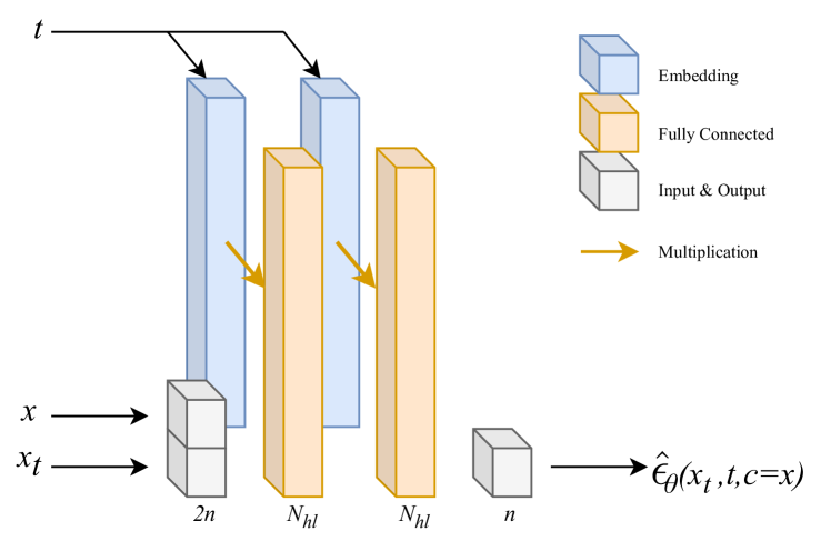
Figure 1: The architecture of the diffusion model is visualized.

II-D Diffusion Noise Scheduling for Zero SNR and $v$ Prediction

The recent work [25] pointed out that for finite $T$ and small $\beta_{t}$, the diffused sample distribution has a nontrivial difference from the white noise distribution. This causes the signal-to-noise ratio (SNR) of the diffusion to be nonzero. More specifically, from (5), the SNR of diffusion is given by $\frac{\bar{\alpha}_{T}}{1-\bar{\alpha}_{T}}$; for instance, for $T=100$ and $\beta_{t}=0.05$ for all $t$, the SNR equals $5.96\times 10^{-3}$. Although this is a relatively small value, it is nonetheless nonzero. In the field of computer vision, eliminating this discrepancy could improve the coverage of samples, as suggested by [25]. One proposed solution is to enforce a 0-SNR diffusion by setting $(1-\bar{\alpha}_{T})\!=\!1$ in (4), implying $\alpha_{T}\!=\!\bar{\alpha}_{T}\!=\!0$ and $\beta_{T}\!=\!1$. However, this adjustment needs a change in parametrization because the diffusion step (3) at $t\!=\!T$ is simplified to $x_{T}\sim\mathcal{N}(0,{I}_{n})$, removing any information about $x_{T-1}$ and $x_{0}$ from $x_{T}$. Consequently, since $x_{T-1}$ and $x_{T}$ are statistically independent, the conditional distributions (2) and (9) reduce to $q(x_{T}|x_{T-1})=q(x_{T})$ and $q(x_{T-1}|x_{T},x_{0})=q(x_{T-1}|x_{0})$, respectively.

In the conventional diffusion model, and more essentially, with $\epsilon$ prediction, the original sample $x_{0}$ is predicted using the diffusion chain (5). However, this approach becomes invalid when the chain is disrupted at $t=T$. Hence, to learn the distribution $q(x_{T-1}|x_{0})$, we require a new parametrization that includes direct prediction of $x_{0}$, such as $x$ prediction [28] or $v$ prediction [26]. In this paper, we use $v$ prediction to enable 0-SNR $\beta_{t}$ scheduling. The vector $v$ is a combination of $\epsilon$ and $x_{0}$, defined as $v(\epsilon,x_{0})\coloneqq\sqrt{\bar{\alpha}_{t}}\epsilon-\sqrt{1-\bar{\alpha}_{t}}x_{0}$. Accordingly, its prediction $\hat{v}_{\theta}(x_{t},t)$ is defined as

$$\hat{v}_{\theta}(x_{t},t)\coloneqq\sqrt{\bar{\alpha}_{t}}\hat{\epsilon}_{\theta}(x_{t},t)-\sqrt{1-\bar{\alpha}_{t}}\hat{x}_{\theta}(x_{t},t).$$ (27)

A neural network is then trained to learn $\hat{v}_{\theta}$ by using the following loss function:

$$\mathcal{L}_{v}=\mathbb{E}_{t,\epsilon,x_{0}}\left[||\hat{v}_{\theta}(x_{t},t)-v(\epsilon,x_{0})||_{2}^{2}\right].$$ (28)

For sample generation in the DDPM framework, one can use the following denoising equation:

$$x_{t-1}=\sqrt{\alpha_{t}}x_{t}-\frac{\sqrt{\bar{\alpha}_{t-1}}(1-\alpha_{t})}{\sqrt{1-\bar{\alpha}_{t}}}\hat{v}_{\theta}(x_{t},t)+\sigma_{t}\epsilon.$$ (29)

In the context of DDIM, the denoising equation is:

$$x_{\tau_{i-1}} =\left(\sqrt{\bar{\alpha}_{\tau_{i-1}}\bar{\alpha}_{\tau_{i}}}+\sqrt{(1-\bar{\alpha}_{\tau_{i-1}})(1-\bar{\alpha}_{\tau_{i}})}\right)x_{\tau_{i}}$$ (30)

$$\ +\left(\!\sqrt{\bar{\alpha}_{\tau_{i}}(1\!-\!\bar{\alpha}_{\tau_{i-1}})}\!-\!\sqrt{\bar{\alpha}_{\tau_{i-1}}(1-\bar{\alpha}_{\tau_{i}})}\right)\hat{v}_{\theta}(x_{\tau_{i}},\tau_{i}).$$ (31)

The proofs of these denoising equations can be found in Appendix VI. The inclusion of the condition $c$ can be accomplished similarly to the process detailed in Section II-B.

II-E Neural Network Architecture

For generating images like CIFAR10, CelebA, and LSUN, U-Nets [29] are typically employed in diffusion models [22]. A U-Net first down-samples the input and then up-samples it, leveraging some skip connections. This forms a U-shaped block diagram, using convolutional layers for both down-sampling and up-sampling. U-Net could be beneficial for a high-dimensional channel where there is interference between dimensions. However, in this paper, we focus on simple memoryless channel models with a small block length $n$. For this, we simply utilize a basic linear network as provided by [30] and modify it for a conditional generation.

Fig. 1 illustrates the generic NN structure used in this paper. It is a feed-forward NN of two fully-connected hidden layers, each having $N_{hl}$ nodes. The input layer takes a noisy sample $x_{t}$ and the channel input $x$, and the NN produces the noise component $\hat{\epsilon}_{\theta}(x_{t},t,c=x)$. Instead of training $T$ distinct models for each time step, the NN typically includes embedding layers for $t$ to function across all $t$. We define an embedding layer of $t$ for each hidden layer with the matching size and multiply it to the hidden layer as demonstrated in Fig. 1. The result of the multiplication is activated by the Softplus function for every hidden layer. The output layer is a linear layer.

We feed the channel input $x$ into the NN as an input for two main reasons: to conditionally generate the channel output via the diffusion model and to ensure that the generated channel output is differentiable with respect to the channel input. This last aspect allows us to form a differentiable backpropagation path for the encoder NN. More specifically, in the diffusion model, the backward step $p_{\theta}(x_{t-1}|x_{t},c)$ follows a normal distribution. The mean of this distribution satisfies (19), which only involves scaling and addition of $x_{t}$ and $\hat{\epsilon}_{\theta}(x_{t},t,c)$. With this construction, the chain rule can be applied without issues when obtaining the partial derivatives of the channel output with respect to the channel input, i.e., during backpropagation for training the encoder NN. The condition $c$ can be defined differently depending on the E2E training algorithm, which is explained further in Section III-B.

III End-to-end Framework and Algorithms

This section defines the E2E framework, which consists of an AE-based channel encoder and decoder with a generative model implemented between them to replace the channel block. Subsequently, we explain two training algorithms for these E2E frameworks, along with their respective advantages and disadvantages.

III-A E2E Channel Coding Framework

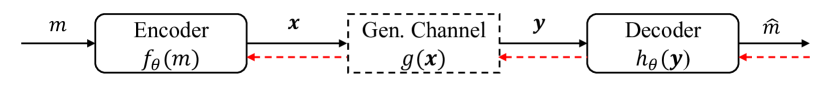
(a) Training the encoder by using the generated channel. The dashed red arrows show the backpropagation path.

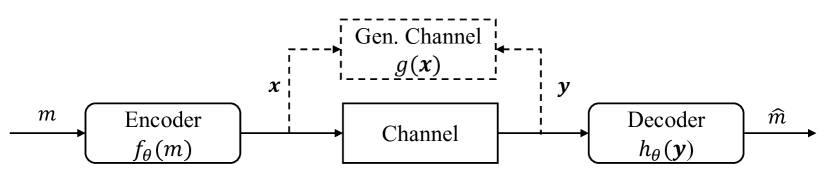
(b) Encoder-specific training of the generative model.

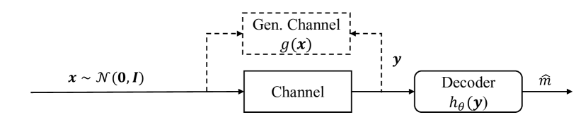
(c) Training the generative model with random channel input.

Figure 2: Block diagrams of the E2E framework.

Consider an AE model where a generated channel is embedded in between the encoder and the decoder blocks, replacing the real channel as depicted in Fig. 2(a). The encoder $f_{\theta}$ maps each one-hot-encoded message, labeled by $m\in\{1,2,\dots,M\}$, to a codeword in an $n$-dimensional real vector space, i.e., $f_{\theta}(m)\in\mathbb{R}^{n}$. We use an NN whose input and output layers have $M$ and $n$ nodes, respectively, with several hidden layers in between. The encoder model’s output is normalized to prevent diverging and to satisfy the power constraint. We denote the generated channel output as $g(f_{\theta}(m))\in\mathbb{R}^{n}$, which is sampled from the generative model. The decoder $h_{\theta}$ mirrors the encoder’s structure, taking $n$-dimensional real vectors and producing $M$ values indicating the predicted likelihood of each message, i.e., $h_{\theta}\left(g(f_{\theta}(m))\right)\in(\mathbb{R}^{+})^{m}$.

It is worth noting that the decoder can be trained independently of the channel’s differentiability. However, training the encoder necessitates a differentiable channel model. To meet this requirement, we utilize the generated channel from the diffusion model, which is differentiable (and can form a backpropagation path) as shown in Fig. 2(a). The AE model is trained to minimize the cross entropy of the one-hot-encoded message and the decoder output, i.e.,

$$\mathcal{L}_{AE}\!=\!\mathbb{E}_{m\sim p(m)}\left[-\sum_{i=1}^{M}\mathbbm{1}_{i=m}\log\left(h_{\theta}\left(g\left(f_{\theta}(m)\right)\right)\right)_{i}\right],$$ (32)

where $\mathbbm{1}$ is the indicator function. During the AE’s training, the generated channel function $g$ remains fixed, optimizing only the parameters of the AE. The encoder and decoder can be trained jointly or in an iterative manner. When the encoder and decoder are jointly optimized during the whole training, it is beneficial to optimize the decoder individually at the end of the training with the encoder fixed, as empirically observed in our simulations. Similarly, during the training of the diffusion model using the loss function (18), only the parameters within the diffusion model are optimized while the AE remains fixed. For the training of the generative model, the encoder’s codewords can be used as shown in Fig. 2(b), or randomly generated channel inputs can be used as illustrated in Fig. 2(c). In the next subsection, we outline the alternation between training the AE and the diffusion model, as well as two different training methods of the diffusion model depending on the training dataset.

III-B E2E Training Algorithms

We consider two E2E training algorithms: the iterative training algorithm and the pre-training algorithm. The former trains the generative model and the AE iteratively, while the latter trains the generative model extensively with random channel inputs before optimizing the AE. The iterative training algorithm is commonly used in the literature for learning E2E channel coding with a generative NN [8, 7, 9, 1].

The generative models are trained with the encoder-specific dataset, comprised of a set of randomly sampled $M$ encoded channel inputs, following the message distribution, and the corresponding channel outputs, as depicted in Fig. 2(b). The diffusion model, which only has to generate a finite number of distributions, can benefit from leveraging the message index to enhance the conditional generative performance. For example, our previous paper [1] defines $c=(m,f_{\theta}(m))$ and multiplies embedding layers of $m$ to each hidden layer as well as the embedding layers of $t$ as shown in Fig. 1. Though this process is not mandatory and increases the model complexity compared to models without embedding layers, it can be useful when conditioning does not perform optimally.

The encoder is then trained with the generated channel outputs. This process is repeated until the AE converges and the E2E SER reaches an acceptable level. When the generative network is trained with the encoder-specific dataset, the generative model only needs to learn $M$ different channel output distributions $p(Y^{n}|X^{n}=f_{\theta}(m))$ for $m\in\{1,2,\dots,M\}$, simplifying the task compared to learning the channel output distribution for arbitrary channel inputs. Hence, the iterative training algorithm requires a generative model with a relatively lower learning capacity, compared to the pre-training algorithm. However, its drawbacks include extensive training time and unstable convergence. Since the generative model is encoder-specific, frequent updates are required when changes occur in the encoder. Otherwise, the generated channel output can significantly deviate from the ground truth, misguiding the encoder. The utility of the generative model is also limited, as it is only compatible with the encoder used during training.

Given these shortcomings, we propose a pre-training algorithm, where the generative model is thoroughly trained once with arbitrary channel inputs and the corresponding channel output distributions. Specifically, we use the isotropic standard normal distribution to generate random channel inputs, as illustrated in Fig. 2(c). In this scenario, the condition $c$ is naturally defined as $c=x$. As the training data $x$ is not associated with any messages or their codewords, it is no longer possible to use embedding layers of $m$ for conditioning the model. The AE is then trained with the pre-trained diffusion model until convergence. The main advantage of the pre-training algorithm is the reduced training time of the E2E framework. Additionally, the trained generative model learns $p(Y^{n}|X^{n})$ for all $X^{n}$ in its domain, enabling its reuse for other applications. The potential challenge lies in the increased need for the generative model’s learning capacity to comprehensively learn the channel behavior and to generalize effectively to out-of-sample scenarios.

Both E2E training algorithms present pros and cons, which we investigate through experiments with different channel models in the following section. To the best of our knowledge, the iteration-free E2E training algorithm has not been used in E2E channel coding studies.

Figure 3: The generative performance of the diffusion model is tested for an AWGN channel with $16$-QAM modulated symbols and $E_{b}/N_{0}=\qty{5}{}$. The constellation of channel output is drawn with $100$ samples for each message. For $m=4$, the histogram and empirical CDF of the channel output’s norm are obtained with $10^{4}$ samples and compared. In the histogram, the frequency indicates the occurrence of the values in the interval among $10^{4}$ samples.

IV Simulation Results

We evaluate first the channel generation of diffusion models and then the E2E communication performance with the diffusion models across different channel scenarios: an AWGN channel, a real Rayleigh fading channel, and an SSPA channel. In all experiments, we assume the messages to be uniformly distributed. The architectures of the AEs and diffusion models follow the structure detailed in Section III-A, but we individually tune the number of hidden layers and hidden nodes for each channel model. For hyperparameters, $T=100$ is used for all diffusion models, and we use the optimal $\beta_{t}$ scheduling identified through our hyperparameter search in Section V-B.

IV-A Channel Generation: 16-QAM for AWGN Channel

This subsection demonstrates the channel generative performance of the conditional diffusion model through an experiment with a 16-ary quadrature amplitude modulation (QAM) and an AWGN channel with $E_{b}/N_{0}=\qty{5}{}$. The AWGN channel is defined as $Y^{n}=X^{n}+Z^{n}$, where $X^{n}\in\mathbb{R}^{n}$ is the channel input, and $Z^{n}$ is the independent channel noise that follows $Z^{n}\sim\mathcal{N}(0,\sigma^{2}{I}_{n})$ for some $\sigma>0$. We employed normalized 16-QAM symbols for channel input and set the $\sigma$ value such that $E_{b}/N_{0}=\qty{5}{}$.

For the diffusion process, we set $T=100$ and used a sigmoid-scheduled $\beta_{t}$ increasing from $10^{-3}$ to $0.05$, i.e., $\beta_{t}=0.001+0.05\left(\frac{1}{1+\exp(-(1+12(t-1)/T))}\right)$. We implemented the conditional diffusion model outlined in Section II-E, with $N_{hl}=110$. The diffusion model was optimized using an accelerated adaptive moment estimation (Adam) optimizer, with a learning rate of $10^{-3}$, dataset size of $10^{6}$, batch size of $100$, and 5 epochs. We used channel inputs following the standard isotropic normal distribution and the corresponding channel outputs as the training dataset, consistent with the pre-training algorithm.

Fig. 3 offers a visual comparison of the constellations of the channel outputs for both the channel model and for the generated channel (in the first two subfigures from the left), demonstrating notably similar distributions. The conditioning capability is proved by the channel output distributions generated for each message. To further verify the distribution, we generated the histogram and empirical cumulative density function (CDF) of the channel output’s magnitude, using $10^{4}$ samples for each message. To conserve space, only the graphs corresponding to $m=4$ are shown in Fig. 3. Both graphs underscore that the generated distribution mirrors the true distribution almost precisely, with analogous results found for other messages as well.

In our prior publication, [1], we conducted a similar experiment but with a different diffusion model and training algorithm. The NN featured three hidden layers with $64$ neurons, each multiplied by embedding layers of $m$ and $t$, and it was trained with encoded symbols and their respective channel outputs. Despite these changes, it is still possible to generate high-quality samples using normally distributed channel inputs for training, and an NN architecture that omits the embedding layers of $m$. This effectively demonstrates the potential of the pre-training algorithm to serve as a substitute for the encoder-specific iterative training algorithm.

Figure 4: The E2E SER for varying $E_{b}/N_{0}$ values is tested for the frameworks trained with an AWGN channel and generated channels.

IV-B E2E Learning: AWGN Channel

TABLE I: The Architecture of the AE used for Simulations.

	Encoder			Decoder
layer	1	2	3	1	2-3	4
neurons	M	M	n	n	M	M
activation	-	ELU	-	-	ELU	-

In this subsection, we present the E2E SER of the frameworks with DDPMs obtained through both iterative training and pre-training algorithms, comparing them with the AEs trained with a known channel model and a generated channel using a WGAN. For the AWGN channel E2E learning experiment, we set $n=7$, $M=16$ and trained the models at $E_{b}/N_{0}=\qty{5}{}$. The channel input in the AE model is defined as $X^{n}=f_{\theta}(m)$ by the encoder’s output, and the channel output $Y^{n}$ is decoded as $h_{\theta}(Y^{n})$.

Given that an AWGN channel is essentially the simplest channel model, only adding Gaussian noise, we employed straightforward NN models to define the encoder and the decoder. These models consist of linear layers with $M=16$ neurons, activated by exponential linear unit (ELU) activation. Table I provides further details on the architecture. The encoder and the decoder were trained simultaneously by using a Nesterov-accelerated adaptive moment estimation (NAdam) optimizer with a learning rate of $10^{-3}$.

Incorporating the outcome of our preceding study [1], we utilize the result of a DDPM trained through an iterative training algorithm. For pre-training, we apply the diffusion model architecture defined in Section II-E, with the parameters $N_{hl}=110$, $T=100$ and cosine scheduled $\beta_{t}$, as proposed in [28]. This setup prescribes that $\bar{\alpha}_{t}=f(t)/f(0)$ where $f(t)=\cos\left(\frac{t/T+s}{1+s}\cdot\frac{\pi}{2}\right)^{2}$ with $s=0.008$. It is important to note that $\bar{\alpha}_{T}=\cos(\pi/2)^{2}=0$ implies a 0-SNR $\beta_{t}$ scheduling. Consequently, the $v$ prediction, as explained in Section II-D, is used. The training uses an Adam optimizer with a learning rate of $10^{-4}$, a dataset size of $10^{7}$, a large batch size of $5000$ to minimize intra-batch variance from the true distribution, and $30$ epochs. The AE is trained for $50$ epochs using a dataset of $10^{6}$ samples and a batch size $100$.

The E2E SER is evaluated for integer values of $E_{b}/N_{0}$ from $\qtyrange{2}{8}{}$ and is illustrated in Fig. 4. Here, the labels ‘DDPM Itr’ and ‘DDPM PreT’ denote the iterative and pre-training algorithms, respectively. In addition to these DDPM-based frameworks, we implemented two other E2E frameworks: Model-Aware and a channel generated through WGAN. Model-Aware directly uses the simulated channel output for training the AE, and its SER curve represents our target. For the WGAN’s generator and critic, we employed NNs with two linear hidden layers, each with 128 nodes, and activated by the rectified linear unit (ReLU). Both the generator and the critic models’ input layers receive the channel input, ensuring model differentiability. The models are trained by the pre-training algorithm: the training dataset consists of randomly generated channel inputs and their channel outputs. We used a root-mean-square propagation (RMSprop) optimizer for them with learning rate $10^{-4}$ and batch size $5000$ across $20\ 000$ iterations. The AE is then trained for 10 epochs using a dataset size of $10^{7}$.

As shown in Fig. 4, SER values decrease with increasing $E_{b}/N_{0}$, yielding concave curves. Both DDPMs and the WGAN generally exhibit SER values close to the target curve, with the DDPM PreT yielding the smallest deviation. As $E_{b}/N_{0}$ increases, the gap on the semi-log plot increases for the WGAN curve but decreases for the DDPM curves.

The results underscore the potential of the DDPM pre-training algorithm to deliver competitive E2E SER performance, occasionally surpassing the iterative training algorithm. This suggests the diffusion model’s ability to learn not only $M$ distinct distributions but also the channel itself for an arbitrary input. While the results are significant, it’s important to caution that these do not guarantee superior performance from the pre-training algorithm in every instance. The optimal design and hyperparameters of the DDPM differ across the two algorithms, complicating direct comparisons. However, the findings remain relevant, indicating that an optimized pre-training algorithm can outperform the iterative algorithm.

Figure 5: The E2E SER for varying $E_{b}/N_{0}$ values is tested for the frameworks trained with a Rayleigh fading channel and generated channels.

IV-C E2E Learning: Rayleigh Fading Channel

We consider a real Rayleigh fading channel, defined by $Y^{n}=H^{n}\circ X^{n}+Z^{n}$, where $\circ$ symbolizes the element-wise multiplication operator, and $H^{n}$ satisfies the condition $\Pr(H_{i}=x;\sigma_{R})=\frac{x}{\sigma_{R}^{2}}\exp(-x^{2}/(2\sigma_{R}^{2}))$ for $x>0$, $\sigma_{R}>0$, and for all $i=1,2,\dots,n$. The additive noise $Z^{n}$ is identically defined as in Section IV-A. We assume a real Rayleigh fading channel with $n=7$, $\sigma_{R}=1$ for $M=16$ messages, and the models were trained at $E_{b}/N_{0}=\qty{12}{}$. The AE model’s architecture is consistent with the one used for the AWGN channel in Section IV-B.

Fig. 5 presents the test SER values of the E2E framework proposed herein, which incorporates diffusion models under two distinct training algorithms. This is compared against the Model-Aware and WGAN frameworks. The SER curve of DDPM Itr is reused from our previous work [1]. The diffusion model for the pre-training algorithm, defined with $N_{hl}=128,T=100,\beta_{t}=0.05$ for all $t$, was trained using the $\epsilon$ prediction method. The training parameters involved a dataset size of $10^{7}$, batch size of $5000$, $30$ epochs, and a learning rate of $10^{-4}$. The AE was trained with a dataset size of $10^{6}$, batch size of $100$, an initial learning rate of $10^{-3}$ for the first $30$ epochs, and then reduced to $10^{-4}$ for the subsequent $60$ epochs. For each epoch, the decoder and encoder were trained successively.

The WGAN model was similarly defined to the one described in Section IV-B and differs only in having 256 neurons per hidden layer and a learning rate set at $5\text{\times}{10}^{-5}$. For the WGAN and the Model-Aware cases, the AE was trained with a dataset of $10^{7}$ samples, a batch size of $1000$, a learning rate of $10^{-3}$, and $10$ epochs.

Model testing was carried out for integer $E_{b}/N_{0}$ values ranging from 125. At the training $E_{b}/N_{0}$ value of 12, all three curves of the generated channels have similar SERs, with the WGAN slightly outperforming the DDPM curves. In the semi-log scale plot, the SER curves of DDPMs and Model-Aware frameworks decrease linearly, while the WGAN curve, maintaining a minuscule gap, aligns with the optimal curve until around 17, where it begins to diverge. Such a limitation is consistent with the GAN results observed in [5]. The gap between the WGAN’s curve and the optimal curve is smaller in the low $E_{b}/N_{0}$ region than that of DDPMs’, whereas the DDPMs outperform the WGAN in the high $E_{b}/N_{0}$ region and continue to decrease in parallel with the target curve. This suggests that the diffusion model provides better generalization for high $E_{b}/N_{0}$ values.

Similarly to the AWGN channel experiment, the pre-training algorithm yields lower SER values compared with DDPM Itr as reported in [1]. Since the experimental settings of the iterative training algorithm in [1] are not identical to those of the pre-training algorithm in this paper, it is not assured that the pre-training algorithm will consistently give better results. However, the results still indicate that the pre-training algorithm can achieve comparable, or even better results than the iterative algorithm. Moreover, pre-training algorithms are preferred as they essentially learn the channel behavior and yield reproducible outcomes. Also, they require less training time without the iterative algorithm. In contrast, the iterative algorithm carries uncertainties concerning the number of samples required for convergence and exhibits variance in the reproduction of results.

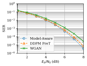
Figure 6: The E2E SER for varying $E_{b}/N_{0}$ values is tested for the frameworks trained with an SSPA channel and generated channels.

IV-D E2E Learning: SSPA Channel

In order to test the performance of diffusion models on a channel model with nonlinear amplification, we utilized the SSPA channel model proposed by [31]. In this model, an $n_{c}$-dimensional complex channel input signal $X^{n_{c}}\in\mathbb{C}^{n_{c}}$, characterizes the SSPA channel as $Y^{n_{c}}=P^{n_{c}}\left(X^{n_{c}}\right)\circ X^{n_{c}}+Z^{n_{c}}$, where $P^{n_{c}}\left(X^{n_{c}}\right)\!=\!(P(|X_{1}|),P(|X_{2}|),\dots,P(|X_{n_{c}}|))\!\in\!\mathbb{R}^{n_{c}}$ is a nonlinear power amplification, and each element $Z_{i}$ of $Z^{n_{c}}$ satisfies $Z_{i}\sim\mathcal{CN}(0,\sigma^{2})$. The power amplification function of an SSPA model is defined as

$$P\left(|X_{i}|\right)=\frac{v}{\left(1+\left[\frac{v\lvert X_{i}\rvert}{A_{0}}\right]^{2p}\right)^{\frac{1}{2p}}}$$ (33)

for some $p>0$, $A_{0}\geq 0$, and $v\geq 0$ for all $i=1,2,\dots,n_{c}$. This function amplifies the signal proportionally to $v$, and the amplification becomes saturated when $\lvert X_{i}\rvert$ is approximately equal to $A_{0}$. The saturation level’s smoothness is determined by $p$: a smaller $p$ results in smoother saturation. For $p\to\infty$, the curve of $P(X_{i})$ increases linearly up to $\lvert X_{i}\rvert=A_{0}$ and stays constant for $\lvert X_{i}\rvert>A_{0}$. This saturation behavior induces the amplification nonlinearity as $P(|X_{i}|+a|X_{j}|)\neq P(|X_{i}|)+aP(|X_{j}|)$ for arbitrary $|X_{i}|$, $|X_{j}|$, and $a\in\mathbb{R}$.

For simulations, parameters were set to be $M=64$, $n_{c}=4$, $p=3$, $A_{0}=1.5$, $v=5$, and $E_{b}/N_{0}=\qty{6}{}$ for training. We used $n=2n_{c}$ real values to represent $n_{c}$-dimensional complex vectors. Fig. 6 illustrates the test SER curves of AEs trained with the SSPA channel model and the synthetic channels created by a diffusion model and a WGAN. The AEs in all scenarios follow the specifications outlined in Table I.

For the Model-Aware case, training was done with a dataset size of $10^{6}$, a batch size of $1024$, and learning rates of $10^{-3},10^{-4},10^{-5}$ for epochs $20$, $40$, $100$ respectively. In the DDPM PreT case, the diffusion model architecture mirrored the one used for an AWGN channel in Section IV-B, except for $\beta_{t}$ scheduling. From a hyperparameter search, the 0-SNR cosine-scheduled $\beta_{t}$ and the corresponding $v$ prediction for denoising were found to be the most effective. The diffusion model was trained using the pre-training algorithm with a dataset size of $10^{7}$, a batch size of $4096$, and learning rates of $10^{-4},10^{-5},10^{-6}$ for $20$, $40$, $100$ epochs respectively. Thereafter, the AE is trained with dataset size $10^{6}$, batch size 128, learning rate $10^{-3},10^{-4}$ for $20$, $40$ epochs respectively.

The WGAN model used for the Rayleigh fading channel with 256 hidden nodes was employed, with modifications made to the input and output layer sizes. A WGAN with 128 hidden nodes was also tested, but a noticeable performance gap existed compared to the larger model with 256 hidden nodes. The WGAN was trained with a batch size of $5000$ and learning rates of $10^{-4}$, $10^{-5}$, $5\times 10^{-6}$, $10^{-6}$ for $\{1,2,2,8\}\times 10^{4}$ iterations, respectively. Thereafter, the AE was trained with a dataset size of $10^{8}$, a batch size of $1000$, and learning rates of $10^{-4},10^{-5},5\times 10^{-6},10^{-6}$ for $40$, $30$, $20$, $70$ epochs, respectively.

As Fig. 6 indicates, the diffusion model achieves a near-optimal performance, while the WGAN still demonstrates a clear gap to the target curve. This suggests that the diffusion model can effectively learn a nonlinear channel distribution as a black box and enable the neural encoder in the E2E framework to learn an almost-optimal codebook.

TABLE II: Dimensionality of the NNs in the Experiments.

	AWGN	Rayleigh	SSPA
DDPM Itr	22 407	22 407	-
DDPM PreT	36 637	74 247	60 178
WGAN G	17 410	67 586	72 200
WGAN C	17 410	67 329	70 401

IV-E Model Complexity Analysis

Table II presents the number of parameters utilized in each simulation. During training, we observed that in order to adequately learn the Rayleigh fading channel and the SSPA channel for E2E learning, both the DDPM and the WGAN required larger NNs compared to the AWGN channel. The smaller networks used for the AWGN channel did not yield satisfactory SER curves, prompting us to increase the number of parameters. This adjustment aligns with expectations, as the AWGN channel output resembles the random seed of generative models, which is generally easier to generate than the other two channel models.

Compared to the iterative training algorithm of DDPM, the pre-training algorithm required larger networks to achieve comparable SERs for both the AWGN channel and the Rayleigh fading channel. For iterative training, the generative model only needs to learn $M$ distributions, whereas, for pre-training, it must learn a general channel distribution for any given arbitrary channel input $x$. As such, this increased model complexity seems unavoidable yet justifiable when seeking more stable training and lower SERs.

In this paper, the WGANs are assessed solely with the pre-training algorithm. For an AWGN channel, the DDPM uses a larger dimensionality than the WGANs but attains superior test SERs for all $E_{b}/N_{0}$ values. Thus, it can be seen as a higher-cost scheme offering enhanced performance. For the Rayleigh fading channel, the DDPM employs far fewer parameters compared to the WGAN model, resulting in comparable results: the WGAN excels in a low SNR region, and the DDPM surpasses it in a high SNR region. For the nonlinear SSPA model, the DDPM achieves better test SER with a significantly smaller NN. Taking all factors into account, the DDPM with the pre-training algorithm offers comparable or better complexity cost-effectiveness depending on channel models.

V Performance Enhancement

To address the slow sampling issue inherent in diffusion models, we investigate the potential time savings and the consequent impact on sample quality when using DDIMs. This subsection analyzes the trade-off between sampling time and sample quality. We accomplish this by comparing the E2E communication quality achieved with DDPMs and DDIMs. Furthermore, we explore optimization of the $\beta_{t}$ parameter as a strategy to improve this trade-off.

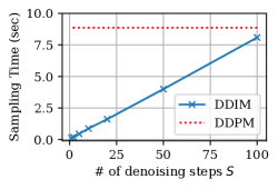
Figure 7: The sampling time vs. the trajectory length $S$. For measurement, $2^{17}=132\ 072$ samples were pulled for each data point, and one NVIDIA RTX 2060 GPU was used.

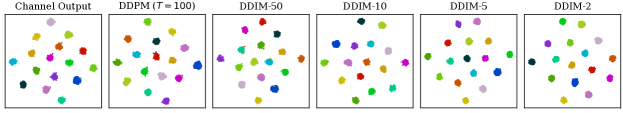
(a) A cosine scheduled $\beta_{t}$ and $v$ prediction are used for the diffusion models.

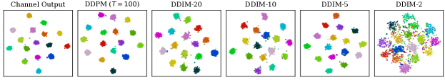
(b) A sigmoid scheduled $\beta_{t}$ and $\epsilon$ prediction are used for the diffusion models.

Figure 8: 2-dimensional visualization of the channel output constellations by using t-SNE.

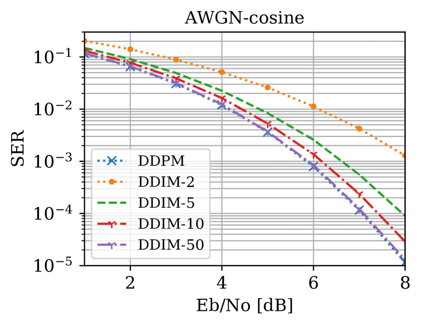
(a) Cosine-scheduled $\beta_{t}$ and $v$ prediction.

(b) Sigmoid-scheduled $\beta_{t}$ with $\epsilon$ prediction.

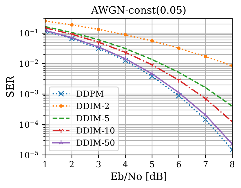
(c) Constant $\beta_{t}=0.05$ with $\epsilon$ prediction.

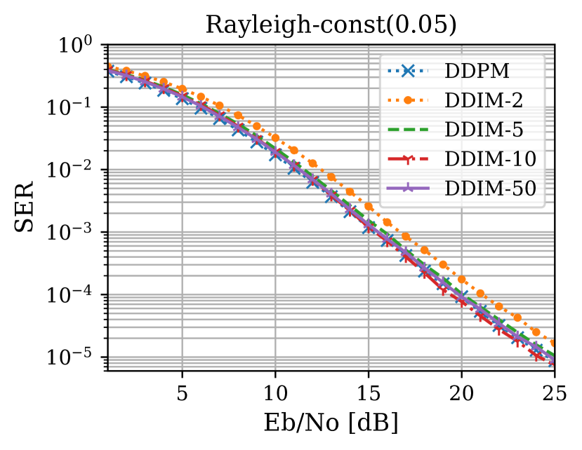
(d) Constant $\beta_{t}=0.05$ with $\epsilon$ prediction.

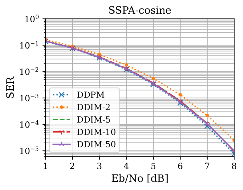
(e) Cosine-scheduled $\beta_{t}$ with $v$ prediction.

Figure 9: The E2E SER is evaluated for different sampling algorithms of diffusion models, i.e., DDPM and DDIM with $S=2,5,10,50$. All these models are trained by the pre-training algorithm.

V-A Sampling Acceleration by DDIM – Trade-off Analysis

The acceleration of diffusion model sampling can be achieved using the DDIM sampling algorithm, as outlined in Section II-C. This subsection examines the trade-off between the sampling speed and sample quality for different values of $S$, focusing on the AWGN channel as discussed in Section IV-B. Sampling speed is measured by the time taken to generate $2^{17}$ samples.

We have illustrated the sampling times of DDPM and DDIM for various values of $S$ ranging from $1$ to $T=100$ in Fig. 7. As expected, the sampling time increases linearly with $S$ and aligns with the DDPM’s sampling time when $S$ is around $T$. This is due to the repetition of the denoising process $S$ times. Notably, even when $S=100$, DDIM is faster than DDPM, presumably because the denoising process in DDPM involves random sampling of $\epsilon$, whereas DDIM’s denoising process is deterministic. By using DDIM the sampling time can be drastically saved. For example, when $S=10$, the sampling time can be reduced by $90.18\%$ compared with DDPM.

Sample quality is assessed using two-dimensional representations of channel outputs generated by the t-distributed stochastic neighbor embedding (t-SNE), as well as the E2E SER performance obtained with DDIM sampling. As a widely used non-linear dimensionality reduction technique, t-SNE visualizes multidimensional data in two- or three-dimensional images by mapping data points based on their Euclidean distances. We utilized the diffusion simulation from Section IV-B for both DDPM and DDIM sampling.

In Fig. 8(a), the seven-dimensional channel outputs and sampled channel outputs are mapped and visualized using t-SNE. We tested DDPM and DDIMs with $S=2,5,10,50$, using 100 samples for each message symbol, which is encoded by the DDPM-trained encoder. Each distinct message is color-coded. The t-SNE mapping is designed to cluster similar data points, resulting in overlaps indicating the closeness or proximity of data points. Channel output, DDPM, DDIM-50, and DDIM-10 present several points clustered with other colors, whereas DDIM-5 and DDIM-2 have perfectly classified symbols due to the less noisy sample distributions generated. However, the t-SNE visualizations do not adequately depict the quality degradation since the original channel output is well-clustered by t-SNE, and the difference is not significant.

To further evaluate DDIMs, we measured the E2E SER for DDIMs with various $S$ values and plotted the results in Fig. 9(a). The E2E framework for each case was trained with the pre-training algorithm: one DDPM model was trained, and AEs were trained with samples drawn using the DDPM sampling algorithm and the DDIM’s accelerated sampling algorithms with $S=2,5,10,50$, respectively. The same NN architecture and hyperparameters were used as in the DDPM PreT case of Section IV-B for comparison.

In Fig. 9(a), the lowest SER values for all $E_{b}/N_{0}$ are achieved by DDPM and DDIM with $S=10$, with DDIM’s SER increasing for smaller $S$ values. DDIM with smaller $S$ values generate distributions with smaller variances, seemingly impeding the AE’s ability to overcome the channel noise. As a lower $S$ value reduces the sampling time but increases the SER, this constitutes a trade-off. Specifically, the sampling time, which significantly influences the training time of the AE, and the E2E communication quality are the factors involved in this trade-off.

V-B Diffusion Noise Scheduling

In our previous paper [1], we adopted a constant $\beta_{t}$ for all $t$ for simplicity. To scrutinize the influence of $\beta_{t}$, we evaluated two $\beta_{t}$-scheduling schemes, cosine and sigmoid scheduling, using an AWGN channel. We assessed them by the quality of their samples and the E2E SER. The cosine scheduling method, as explained in Section IV-B, and the sigmoid scheduling, as detailed in Section IV-A, were utilized. Fig. 8 presents a comparison of these two scheduling methods by using two-dimensional t-SNE-mapped images of generated channel outputs. Unlike the cosine scheduling, demonstrated in Fig. 8(a), the sigmoid scheduling samples (shown in Fig. 8(b)) appear more misclassified as $S$ decreases. This discrepancy likely arises because the cosine scheduling is coupled with $v$ prediction, which entails direct prediction of $\hat{x}$ by samples. This combination allows the diffusion model to generate fine samples despite substantial skips in the sampling process. Conversely, the denoising process of $\epsilon$ prediction relies solely on noisy samples, and this generative performance can be noticeably impaired when $S$ is too small.

The E2E test SER is assessed for both scheduling schemes and for constant $\beta_{t}$ in Fig. 9(a) to 9(c) by using both DDPM and DDIMs. Compared to the constant $\beta_{t}$, both scheduling methods improve the test SER for all sampling algorithms, with the performance gap more pronounced for DDIMs with small $S$. In contrast to the sample quality observed in Fig. 8, sigmoid scheduling shows more robustness to DDIM sampling, resulting in a negligible SER degradation even for $S=5$. This likely stems from the added noise from suboptimal sampling, making the AE more robust to channel noise. However, the sample distributions of cosine scheduling become less noisy for smaller $S$, and the AEs are trained with more reliable channels than the channel model, which obstructs learning and amplifies the test error rates.

Remark that optimizing $\beta_{t}$ scheduling can improve the E2E SER in the framework, and the performance gain can be substantial for DDIMs. The optimal $\beta_{t}$ scheduling depends on the targeted error probability. For instance, if the lowest SER is desired regardless of cost, the cosine scheduling method with DDPM is the superior choice. If a small SER increment can be tolerated, the sigmoid scheduling with DDIM-5 would yield the most sampling-time-effective result: the sampling time can be reduced by $94.69\%$ with only 1.16 increase in SER for $E_{b}/N_{0}=\qty{5}{}$, in comparison with DDPM.

Identifying an effective $\beta_{t}$ scheduling without testing the E2E SER for each case is a formidable task. In practice, we utilized plots such as Fig. 3 to examine the sample quality and selected the best among the tried options. For the Rayleigh fading channel and the SSPA channel, a constant $\beta_{t}=0.05$ and the cosine scheduling, respectively, produced the best sample quality among the three methods. Their test SER curves are illustrated in Fig. 9(d) and 9(e). It is important to note that the optimal choice of $\beta_{t}$ can differ for each channel model in terms of robustness to skipped sampling. This underscores the necessity of an experimental search for a suitable $\beta_{t}$, as it depends on the sampling distributions.

VI Conclusion and Outlook

In this paper, we examined a deep learning-based E2E channel coding framework, in which the channel block is synthesized by a conditional diffusion model. Through our simulations, we demonstrated the robust channel generation capabilities of diffusion models and near-optimal E2E SERs within the framework they support. Importantly, unlike several GAN variants, diffusion models were observed not to encounter error floors in high SNR regions.

Addressing the primary shortcoming of the diffusion model—its lengthy sampling process—we utilized the skipped sampling technique from DDIMs to speed up the process. This approach, however, led to a degradation in sample quality as more steps were skipped. We observed that this trade-off can be notably improved by selecting an appropriate noise scheduling through empirical testing.

Our results indicate that with a thoughtful choice of noise scheduling, the sampling time can be reduced considerably with only a marginal increase in SER. For example, in an AWGN channel with $\qty{5}{}$ of $E_{b}/N_{0}$ and employing sigmoid-scheduled noise variance, the sampling time was reduced by $94.69\%$ with only a modest SER increase of $\qty{1.16}{}$.

Our work underscores the potential of diffusion models, with their robust channel generation performance and near-optimal resulting SERs, to significantly bolster the efficacy and efficiency of E2E channel coding frameworks.

The channel models presented in this paper are i.i.d., indicating that they are memoryless and interference-free in both time and frequency domains. These models could be expanded to include those with tapped delays or inter-symbol interferences and could even incorporate real, physically observed channels. The block length used in our tests is relatively small. To manage more complex distributions and support longer block lengths, the architecture of the diffusion model’s network needs to be more robust and scalable, for instance, by adopting structures like U-Nets.

Moreover, for the purpose of this study, we used relatively simple multi-layer perceptrons for encoders and decoders. There are potential improvements to be gained from the use of more advanced encoders and decoders. For instance, it was shown that a neural receiver, designed similarly to traditional channel estimation, could improve error rates for a Rayleigh block fading channel in [10].

As is common in many DL studies, some hyperparameters are still relatively understudied. For instance, the choice of the training $E_{b}/N_{0}$ value in our study was made through a rudimentary grid search, but there could be optimal choices that have not been explored yet.

[Sampling Algorithms for $v$ Prediction]

The DDPM denoising formula for $v$ prediction can be obtained by parameterizing $\mu_{\theta}(x_{t},t)$ in terms of $x_{t}$ and $\hat{v}_{\theta}(x_{t},t)$ in the following equation:

$$x_{t-1}(x_{t},t) =\mu_{\theta}(x_{t},t)\!+\!\sigma_{t}\epsilon.$$ (34)

Equation (13) of $\mu_{\theta}(x_{t},t)$ can be solved by substituting $\hat{x}_{\theta}(x_{t},t)$ by $\hat{x}_{\theta}(x_{t},t)=\sqrt{\bar{\alpha}_{t}}x_{t}-\sqrt{1-\bar{\alpha}_{t}}\hat{v}_{\theta}(x_{t},t)$ as

$$\mu_{\theta}(x_{t},t) \!=\!\frac{\sqrt{\alpha_{t}}(1\!-\!\bar{\alpha}_{t-1})}{1-\bar{\alpha}_{t}}x_{t}\!+\!\frac{\sqrt{\bar{\alpha}_{t-1}}(1\!-\!\alpha_{t})}{1-\bar{\alpha}_{t}}\sqrt{\bar{\alpha}_{t}}x_{t}$$ (35)

$$\quad\quad-\frac{\sqrt{\bar{\alpha}_{t-1}}(1-\alpha_{t})}{1-\bar{\alpha}_{t}}\sqrt{1-\bar{\alpha}_{t}}\hat{v}_{\theta}(x_{t},t)$$ (36)

$$=\frac{\sqrt{\alpha_{t}}}{1-\bar{\alpha}_{t}}\left(1-\bar{\alpha}_{t-1}+\bar{\alpha}_{t-1}(1-\alpha_{t})\right)x_{t}$$ (37)

$$\quad\quad\quad-\frac{\sqrt{\bar{\alpha}_{t-1}}(1-\alpha_{t})}{\sqrt{1-\bar{\alpha}_{t}}}\hat{v}_{\theta}(x_{t},t)$$ (38)

$$=\sqrt{\alpha_{t}}x_{t}-\frac{\sqrt{\bar{\alpha}_{t-1}}(1-\alpha_{t})}{\sqrt{1-\bar{\alpha}_{t}}}\hat{v}_{\theta}(x_{t},t).$$ (39)

The denoising step equation (29) can be completed by plugging in this formula of $\mu_{\theta}(x_{t},t)$ in (34).

The DDIM sampling algorithm with $\epsilon$ prediction is

$$x_{\tau_{i-1}} =\sqrt{\bar{\alpha}_{\tau_{i-1}}}\hat{x}_{\theta}(x_{\tau_{i}},\tau_{i})+\sqrt{1-\bar{\alpha}_{\tau_{i-1}}}\hat{\epsilon}_{\theta}(x_{\tau_{i}},\tau_{i}),$$ (40)

where $\hat{x}_{\theta}$ is calculated by $x_{\tau_{i}}$ based on the diffusion process as in (24). By definition of $v$, we have

$$\hat{x}_{\theta}(x_{t},t)=\sqrt{\bar{\alpha}_{t}}x_{t}-\sqrt{1-\bar{\alpha}_{t}}\hat{v}_{\theta}(x_{t},t)$$ (41)

for all $t$. One can induce a similar formula for $\hat{\epsilon}_{\theta}$ as a function of $x_{t}$ and $\hat{v}_{\theta}(x_{t},t)$, starting from the definition (15):

$$\hat{\epsilon}_{\theta}(x_{t},t) =\frac{1}{\sqrt{1-\bar{\alpha}_{t}}}\left(x_{t}-\sqrt{\bar{\alpha}_{t}}\hat{x}_{\theta}(x_{t})\right).$$ (42)

By plugging in (41) to the above equation, we have

$$\hat{\epsilon}_{\theta}(x_{t},t)$$ (43)

$$= \frac{1}{\sqrt{1-\bar{\alpha}_{t}}}\left(x_{t}-\sqrt{\bar{\alpha}_{t}}\left(\sqrt{\bar{\alpha}_{t}}x_{t}-\sqrt{1-\bar{\alpha}_{t}}\hat{v}_{\theta}(x_{t},t)\right)\right)$$ (44)

$$= \frac{1-\bar{\alpha}_{t}}{\sqrt{1-\bar{\alpha}_{t}}}x_{t}+\sqrt{\bar{\alpha}_{t}}\hat{v}_{\theta}(x_{t},t)$$ (45)

$$= \sqrt{1-\bar{\alpha}_{t}}x_{t}+\sqrt{\bar{\alpha}_{t}}\hat{v}_{\theta}(x_{t},t).$$ (46)

One can substitute $\hat{x}_{\theta}(x_{\tau_{i}},{\tau_{i}})$ and $\hat{\epsilon}_{\theta}(x_{\tau_{i}},{\tau_{i}})$ in (40) by using two equations (41) and (46) for $t=\tau_{i}$, which proves the denoising formula (40) as follows

$$x_{\tau_{i-1}}=\sqrt{\bar{\alpha}_{\tau_{i-1}}}\left(\sqrt{\bar{\alpha}_{t}}x_{\tau_{i}}-\sqrt{1-\bar{\alpha}_{\tau_{i}}}\hat{v}_{\theta}(x_{\tau_{i}},\tau_{i})\right)$$ (47)

$$+\!\sqrt{1\!-\!\bar{\alpha}_{\tau_{i-1}}}\left(\!\sqrt{1\!-\!\bar{\alpha}_{\tau_{i}}}x_{\tau_{i}}\!+\!\sqrt{\bar{\alpha}_{\tau_{i}}}\hat{v}_{\theta}(x_{\tau_{i}},\tau_{i})\right)\!\!$$ (48)

$$= \left(\sqrt{\bar{\alpha}_{\tau_{i-1}}\bar{\alpha}_{\tau_{i}}}+\sqrt{(1-\bar{\alpha}_{\tau_{i-1}})(1-\bar{\alpha}_{\tau_{i}})}\right)x_{\tau_{i}}$$ (49)

$$+\!\left(\!\sqrt{\bar{\alpha}_{\tau_{i}}(1-\bar{\alpha}_{\tau_{i\!-\!1}})}\!-\!\sqrt{\bar{\alpha}_{\tau_{i-1}}(1-\bar{\alpha}_{\tau_{i}})}\right)\hat{v}_{\theta}(x_{\tau_{i}},\tau_{i}).$$ (50)

References

- [1] M. Kim, R. Fritschek, and R. F. Schaefer, “Learning end-to-end channel coding with diffusion models,” in Proc. Int. ITG Workshop Smart Antennas and Conf. Sys., Commun., and Coding, Braunschweig, Germany, Mar. 2023, pp. 208–213.
- [2] T. J. O’Shea, K. Karra, and C. T. Clancy, “Learning to communicate: Channel auto-encoders, domain specific regularizers, and attention,” in Proc. IEEE Int. Symp. Signal Process. Inf. Technol., Limassol, Cyprus, Dec. 2016, pp. 223–228.
- [3] T. O’Shea and J. Hoydis, “An introduction to deep learning for the physical layer,” IEEE Trans. Cogn. Commun. Netw., vol. 3, no. 4, pp. 563–575, Dec. 2017.
- [4] Y. Jiang, H. Kim, H. Asnani, S. Kannan, S. Oh, and P. Viswanath, “Turbo autoencoder: Deep learning based channel codes for point-to-point communication channels,” in Proc. Adv. Neural Inf. Process. Syst., Vancouver, Canada, Dec. 2019, pp. 2754–2764.
- [5] M. V. Jamali, H. Saber, H. Hatami, and J. H. Bae, “ProductAE: Toward deep learning driven error-correction codes of large dimensions,” arXiv preprint arXiv:2303.16424, Mar. 2023.
- [6] H. Ye, G. Y. Li, B.-H. Juang, and K. Sivanesan, “Channel agnostic end-to-end learning based communication systems with conditional GAN,” in Proc. IEEE Globecom Workshops, Abu Dhabi, United Arab Emirates, Dec. 2018, pp. 1–5.
- [7] S. Dörner, M. Henninger, S. Cammerer, and S. ten Brink, “WGAN-based autoencoder training over-the-air,” in Proc. IEEE Int. Workshop Signal Process. Adv. Wireless Commun., Atlanta, GA, May 2020, pp. 1–5.
- [8] T. J. O’Shea, T. Roy, N. West, and B. C. Hilburn, “Physical layer communications system design over-the-air using adversarial networks,” in Proc. Eur. Signal Process. Conf., Rome, Italy, Sep. 2018, pp. 529–532.
- [9] H. Jiang, S. Bi, L. Dai, H. Wang, and J. Zhang, “Residual-aided end-to-end learning of communication system without known channel,” IEEE Trans. Cogn. Commun. and Netw., vol. 8, no. 2, pp. 631–641, June 2022.
- [10] F. A. Aoudia and J. Hoydis, “End-to-end learning of communications systems without a channel model,” in Proc. Asilomar Conf. Signals, Syst., and Comput., Pacific Grove, CA, Oct. 2018, pp. 298–303.
- [11] T. J. O’Shea, T. Roy, and N. West, “Approximating the void: Learning stochastic channel models from observation with variational generative adversarial networks,” in Proc. IEEE Int. Conf. Comput., Netw., and Commun., Honolulu, HI, Feb. 2019, pp. 681–686.
- [12] W. Xia, S. Rangan, M. Mezzavilla, A. Lozano, G. Geraci, V. Semkin, and G. Loianno, “Generative neural network channel modeling for millimeter-wave UAV communication,” IEEE Trans. Wireless Commun., vol. 21, no. 11, pp. 9417–9431, 2022.
- [13] E. Balevi and J. G. Andrews, “Wideband channel estimation with a generative adversarial network,” IEEE Trans. Wireless Commun., vol. 20, no. 5, pp. 3049–3060, Jan. 2021.
- [14] M. Arvinte and J. Tamir, “Score-based generative models for wireless channel modeling and estimation,” in Proc. Int. Conf. Learn. Representations Workshop, Chicago, IL, Apr. 2022.
- [15] J. Zicheng, G. Shen, L. Nan, P. Zhiwen, and Y. Xiaohu, “Deep learning-based channel estimation for massive-MIMO with mixed-resolution ADCs and low-resolution information utilization,” IEEE Access, vol. 9, pp. 54938–54950, 2021.
- [16] E. Balevi, A. Doshi, A. Jalal, A. Dimakis, and J. G. Andrews, “High dimensional channel estimation using deep generative networks,” IEEE J. Sel. Areas Commun., vol. 39, no. 1, pp. 18–30, Nov. 2020.
- [17] F. Weisser, T. Mayer, B. Baccouche, and W. Utschick, “Generative-AI methods for channel impulse response generation,” in Proc. Int. Workshop Smart Antennas, French Riviera, France, Nov. 2021, pp. 65–70.
- [18] T. Orekondy, A. Behboodi, and J. B. Soriaga, “MIMO-GAN: Generative MIMO channel modeling,” in Proc. IEEE Int. Conf. Commun., May 2022, pp. 5322–5328.
- [19] Z. Xiao, K. Kreis, and A. Vahdat, “Tackling the generative learning trilemma with denoising diffusion GANs,” in Proc. Int. Conf. Learn. Representations, Apr. 2022.
- [20] F.-A. Croitoru, V. Hondru, R. T. Ionescu, and M. Shah, “Diffusion models in vision: A survey,” IEEE Trans. Pattern Anal. Mach. Intell., vol. 45, no. 09, pp. 10850–10869, Sep. 2023.
- [21] J. Sohl-Dickstein, E. Weiss, N. Maheswaranathan, and S. Ganguli, “Deep unsupervised learning using non-equilibrium thermodynamics,” in Proc. Int. Conf. Mach. Learn., Lille, France, July 2015, PMLR, pp. 2256–2265.
- [22] J. Ho, A. Jain, and P. Abbeel, “Denoising diffusion probabilistic models,” in Proc. Adv. Neural Inf. Process. Syst., Dec. 2020, pp. 6840–6851.
- [23] Y. Song and S. Ermon, “Generative modeling by estimating gradients of the data distribution,” in Proc. Adv. Neural Inf. Process. Syst., Vancouver, Canada, Dec. 2019.
- [24] Y. Song, J. Sohl-Dickstein, D. P. Kingma, A. Kumar, S. Ermon, and B. Poole, “Score-based generative modeling through stochastic differential equations,” in Proc. Int. Conf. Learn. Representations, May 2021.
- [25] S. Lin, B. Liu, J. Li, and X. Yang, “Common diffusion noise schedules and sample steps are flawed,” arXiv preprint arXiv:2305.08891, July 2023.
- [26] T. Salimans and J. Ho, “Progressive distillation for fast sampling of diffusion models,” in Proc. Int. Conf. Learn. Representations, Apr. 2022.
- [27] J. Song, C. Meng, and S. Ermon, “Denoising diffusion implicit models,” in Proc. Int. Conf. Learn. Representations, May 2021.
- [28] A. Q. Nichol and P. Dhariwal, “Improved denoising diffusion probabilistic models,” in Proc. Int. Conf. Mach. Learn. PMLR, May 2021, pp. 8162–8171.
- [29] O. Ronneberger, P. Fischer, and T. Brox, “U-Net: Convolutional networks for biomedical image segmentation,” in Proc. Int. Conf. Medical Image Comput. Computer-Assisted Intervention, Munich, Germany, Oct. 2015, Springer, pp. 234–241.
- [30] J. R. Siddiqui, “Denoising diffusion model,” https://github.com/azad-academy/denoising-diffusion-model.git, 2022.
- [31] C. Rapp, “Effects of HPA-nonlinearity on a 4-DPSK/OFDM-signal for a digital sound broadcasting signal,” European Space Agency Special Publication, vol. 332, pp. 179–184, Oct. 1991.