Markov Chain Monte Carlo for Bayesian Parametric Galaxy Modeling in LSST
Abstract
We apply Markov Chain Monte Carlo (MCMC) to the problem of parametric galaxy modeling, estimating posterior distributions of galaxy properties such as ellipticity and brightness for more than 100,000 images of galaxies taken from DC2, a simulated telescope survey resembling the upcoming Rubin Observatory Legacy Survey of Space and Time (LSST). We use a physically informed prior and apply selection corrections to the likelihood. The resulting posterior samples enable rigorous probabilistic inference of galaxy model parameters and their uncertainties. These posteriors are one key ingredient in a fully probabilistic description of galaxy catalogs, which can ultimately enable a refined Bayesian estimate of cosmological parameters. We systematically examine the reliability of the posterior mean as a point estimator of galaxy parameters, and of the posterior width as a measure of uncertainty, under some common modeling approximations. We implement the probabilistic modeling and MCMC inference using the JIF (Joint Image Framework) tool, which we make freely available online.
1 Introduction
Because gravitational lensing depends directly on the overall distribution of matter in a given patch of space, it gives a window into the overall structure and evolution of the universe as a whole (Kilbinger, 2015), enabling constraints on e.g. dark energy (LSST Dark Energy Science Collaboration, 2018). Much of the time the effect of lensing is too subtle to be observed in individual galaxies. Rather, so-called “weak lensing” is statistically inferred by analyzing the correlated pattern of measured shapes of multiple galaxies. Increasing the number of well-measured galaxy shapes is generally expected to improve the statistical strength of weak lensing inferences, as long as systematic errors can be controlled (Mandelbaum, 2018).
The Vera C. Rubin Observatory, under construction, is projected to begin the 10 year Legacy Survey of Space and Time (LSST; Ivezić et al. 2019) in 2024. The LSST will observe an unprecedented number of galaxies throughout a wide and deep volume of space. In order to take complete advantage of this dataset for cosmological inference, we are faced with correspondingly unprecedented demands on the mitigation and characterization of systematic uncertainties in galaxy shape measurements. Standard maximum likelihood estimators of galaxy shapes suffer from numerous biases from sources such as noise (Refregier et al., 2012), pixelation, point-spread function (PSF) distortions (Simon & Schneider, 2017), and potentially centroid estimation errors (Tessore, 2017). In addition to its own irreducible contributions to uncertainty, noise bias interacts with and amplifies the effects of model bias, the inability of a given galaxy model to exactly fit the truth (Kacprzak et al., 2014). These sources of bias must be calibrated away using estimator-specific methods (e.g. Tessore 2017), which may still leave behind systematic uncertainties that are not always well understood. In any case, a single point estimate of any value, such as galaxy ellipticity, even when accompanied by a confidence interval, fails to reflect all possible information embedded in one’s limited data set.
In contrast, a Bayesian forward modeling approach need not be similarly subject to the biases noted above—the noise level, PSF, and pixelization effects, plus many other effects on image rendering, can in principle be forward-modeled and thus naturally accounted for without a separate calibration step. Galaxy shape uncertainties can be described in a Bayesian sense by selecting a parametric family of galaxy light profiles, asserting a prior probability distribution on the profile parameters, and then finding the posterior probability distribution over these parameters for any specific observed data instance. Given a sufficiently descriptive model and the ability to compute the full posterior distribution, this approach can make optimal use of all available data. In this study we build on earlier Bayesian parametric galaxy modeling methods to expand the power of this approach and study its effectiveness in the specific context of LSST.
If the model family contains light profiles sufficiently close to the true light distribution of any given galaxy, if the assumed prior is close to the overall distribution of true model parameters in the dataset, if the production of observed images of any given galaxy can be modeled sufficiently well, and if the corresponding posterior can be computed exactly, then the posterior mean will be an unbiased estimator of the model parameters (Miller et al., 2007). In practice, the model family, the assumed prior, the assumed likelihood, and the computed posterior will all be approximations to the truth. In order to study how well our approach can recover true underlying galaxy properties, as well as to examine it in the specific context of LSST, we use images and associated data products from the DC2 simulated sky survey (Abolfathi et al., 2021). By construction, the galaxies in these images have realistically correlated distributions of apparent sizes, morphologies, luminosities, and positions in the sky, and are rendered as they would be perceived by LSST.
We introduce the Joint Image Framework (JIF), a code for handling Markov chain Monte Carlo (MCMC) fits of parametric light profiles to images, with which we fit nearly 150,000 simulated galaxies. As in most previous studies of Bayesian parametric galaxy modeling (e.g. Miller et al. 2007; Kitching et al. 2008), we confine our attention to individual galaxies that do not significantly overlap others and are well-separated from their nearest neighbors. Due to the extreme depth of LSST, such totally “unblended” galaxies will be the exception rather than the rule (Melchior et al., 2021), further motivating the study of galaxy model fitting methods in this specific survey context. Blending notwithstanding, this study still provides a baseline for comparing the performance of our approach with others, along with a foundation for future blending studies. The extension of the current method to more general, blended galaxy images is briefly discussed in the concluding section.
Our overall approach is to iteratively render simulated images of galaxy light profiles with assumed parameters, compare these to the observed telescope image, and thereby compute the likelihood, which together with the prior probability on the assumed parameters informs the progression of the MCMC chain. The premise of computing the likelihood via comparing simulated galaxy image models to real images was laid out in Kuijken (1999) as a way of potentially improving on the Kaiser–Squires–Broadhurst (Kaiser et al., 1995) method for estimating weak lensing shear. This forward image modeling approach was incorporated into Bayesian posterior inference in Im2shape (Bridle et al., 2001, 2013), which was tested alongside other weak lensing estimation methods as part of the Shear Testing Programme (STEP; Heymans et al. 2006). STEP used Source Extractor (Bertin & Arnouts, 1996) to supply the initial detections for all methods. Here, we instead use detections provided by the footprint construction and peak finding algorithms of the LSST Science Pipelines, described in Sections 2 and 3. Our rationale for using Pipelines detections is twofold: first, it is convenient, since a large set of those have already been made and publicly shared, with corresponding truth information, as part of DC2 and Rubin Observatory’s Data Preview 0111https://dp0-1.lsst.io/; more significantly, something close to this exact procedure is likely to be implemented in early LSST data releases.
Whereas JIF, Im2shape, and other methods discussed below use MCMC for posterior estimation, the LensFit (Miller et al., 2007) method instead marginalizes over several model parameters with a combination of analytic and numeric methods, and ultimately evaluates the entire likelihood surface in ellipticity. While this approach is appealing for ellipticity measurements due to its speed, it explicitly makes no attempt to measure the other “uninteresting” parameters, and it relies on significant assumptions on the specific forms of the prior and likelihood in order to make the marginalization tractable. With MCMC the closest corresponding assumption is simply that the prior and likelihood can be computed quickly, which in principle allows more realistic forms for both, so long as sufficient computing resources and efficient algorithms can be brought to bear. In all the preceding methods including JIF, the basic surface brightness profile shape for any particular fit can be freely chosen: the initial LensFit studies focused on an exponential profile (Miller et al., 2007; Kitching et al., 2008). For a single-component light profile of this sort, the parameters needed to specify a given galaxy’s top-of-the-atmosphere appearance in a single photometric band are its total brightness, some measure of its overall size such as the half-light radius, two real numbers describing its lensed ellipticity, and two numbers specifying its position on the sky. We model precisely this set of six parameters, just as in the LensFit studies, though we consider de Vaucouleurs (bulge) in addition to exponential (disk) light profiles.
This galaxy parameterization suffices to capture much of the morphological range in the DC2 simulations, and the minimal number of parameters simplifies the inference, though JIF is designed to readily incorporate other parametric models. For example, functionality already exists in JIF for modeling a generic Sérsic index. Various other Bayesian parametric galaxy modeling codes have been developed in recent years with at least comparable expressivity, including ProFit (Robotham et al., 2017), PyAutoGalaxy (Nightingale et al., 2023), pysersic (Pasha & Miller, 2023), BANG (Rigamonti et al., 2023), and AstroPhot (Stone et al., 2023). All of these implement one or more variants of MCMC. Given the many tools in this ecosystem and the evident demand behind them, it is worth examining how this approach performs across a wide swath of plausible inputs with realistic complications. “Performance” includes such considerations as run time, chain convergence quality, and posterior bias and calibration, all of which we consider here. We look at a greater number of examples, and go into at least as much analytical detail, as any of the aforementioned studies; the most similar efforts are Robotham et al. (2017) and Rigamonti et al. (2023), which present thorough studies of real or realistic simulated data sets consisting of 10,000 galaxies each.222The ProFit study is particularly noteworthy here for examining simulated LSST data. Real data can include such complications as masked pixels, invalid pixel values, pathological variance plane estimates, and pathological photometric calibrations, all of which need to be accounted for in the likelihood model. JIF accommodates all of these and runs to completion without issues on nearly every example in our data set.
Focusing on a specific subset of detected galaxies in a specific sky survey underscores the importance of carefully establishing the prior probability distribution for the model parameters, as well as the corrections that must be made to the likelihood to account for the specific procedures used to identify galaxy images in a given data set. The present study takes the rare step, in the recent literature on Bayesian galaxy modeling in deep optical sky surveys, of explicitly formulating a specific, highly informative prior. A noteworthy exception is the study of Rigamonti et al. (2023) applying BANG to galaxies in the SDSS-MaNGA survey, in which they considered three different priors of varying strength. Stone et al. (2023) distinguish cases of MCMC fitting in which “prior information is to be encoded into the fit,” as opposed presumably to the MCMC results they demonstrate on a test example. In a truly Bayesian interpretation of uncertainty, there is no such thing as not using a prior. Running an MCMC chain without explicitly computing a prior typically means that one is working, implicitly, with a uniform prior across all valid parameter values (within some acceptable range for each value or combination thereof). The resulting posteriors do not take into account all the existing information we in fact have as to what combinations of parameters are more plausible than others. Such posteriors are also highly determined by the likelihood, which in the case of low S/N images can be quite strongly distorted from the truth. In the worst case this can lead to outright fit failures, as seen in Robotham et al. (2017). To study the potential benefits of using a more informed prior, we adopt a prior that matches as closely as possible the true distribution of galaxy properties in our data set.
We also take the novel step, in Bayesian parametric galaxy modeling studies, of developing selection corrections to the likelihood. These are required due to the fact that all data examples we examine in practice must pass a set of selection criteria to be considered, which means that the set of data we see is systematically skewed from what a more naive, unconditioned likelihood model would predict. As we show, both the prior and the selection corrections play dominant roles in determining the posteriors for low S/N galaxies, which are expected to comprise a large fraction of the total number of galaxies detected in LSST. Unlike the SDSS-MaNGA data set used in the BANG study, we consider here many poorly-resolved galaxies with true average brightness levels well below the threshold for detection, which only enter our data set through a chance accumulation of noise in the DC2 images. This is a major reason we adopt such a simple description of galaxy morphology, as opposed to the 18-parameter model used in Rigamonti et al. (2023). Nevertheless, so long as the uncertainties on these galaxies can be modeled reliably, their images can contribute statistical power to weak lensing inference. Hence we concern ourselves here with getting things right across the entire range of observed galaxy fluxes.
The JIF framework directly develops one key component—MCMC samples from the posteriors of galaxies detected in optical telescope images—of the strategy of Schneider et al. (2015) (hereafter S15). The relatively ambitious goal of that approach is to model “all physical parameters that are needed to completely describe the measured pixel values in a photometric survey,” i.e. to develop a fully probabilistic description of the full cosmology-to-images process, and from there use Bayesian inference to constrain the properties of cosmological parameters from the observed telescope images. S15 stated a complete probabilistic model of cosmic shear from this perspective, and took initial steps to develop practical computational approaches to the corresponding cosmological inference problem. As outlined in Figure 9 of S15, that approach begins by looking at the telescope images recorded in a given survey, which are provided by the DC2 simulations in the present study. Processing then proceeds through source identification on these images, accomplished by the Pipelines in our case, and then to what S15 Figure 9 calls a “Reaper” step, which is the specific functionality we develop and study here using JIF. The approach goes on to connect the JIF outputs, which consist of samples from the posterior probability distribution of the parameters for each galaxy considered independently, to subsequent stages of hierarchical inference. These stages use importance sampling to combine the separate galaxy posterior samples from the first step into a common posterior on the weak lensing potential, and then finally a posterior on fundamental cosmological parameters.
A full implementation of the later inference stages based on our JIF outputs is left for future work, but prototype capabilities have been exhibited in various studies. A recent, partial implementation of one of these stages is the hierarchical modeling functionality of PyAutoGalaxy, capable of fitting a consistent model to thousands of galaxies simultaneously (Nightingale et al., 2023), though its specific utility for inferring cosmic shear remains to be seen. Some prototype shear inference capabilities developed for S15 were demonstrated (Mandelbaum et al., 2015) on the GREAT3 community cosmic shear measurement challenge (Mandelbaum et al., 2014). GREAT3 used only idealized data missing much of the complexity of real footprints, which the present study seeks to address. S15 handled the simulation of galaxy images, for likelihood computations, using The Tractor code (Lang et al., 2016). Here we instead use GalSim (Rowe et al., 2015) galaxy image simulation functionality incorporated into JIF. Whereas The Tractor, as used in S15, models both galaxy light profiles and PSFs as sums of 2D Gaussian distributions in order to enable fast analytic convolutions of the two, JIF allows the use of arbitrary parametric forms for both the galaxy light profile and PSF. Here we use single-component bulge and disk profiles as noted above, together with a Kolmogorov form for the PSF defined in GalSim.333See Rowe et al. (2015) for a description of the specific functional forms of the exponential, de Vaucouleurs, and Kolmogorov distributions used in this study. Schneider et al. (2017) adopt a specific Gaussian process prior form developed by Ng (2016) for the weak lensing shear and convergence fields; use this prior to derive an “interim posterior” on said fields given simple estimates, with error bars, of the ellipticities of many galaxies in an image; and develop a couple of sampling algorithms for establishing posteriors on cosmological parameters, starting from the interim weak lensing posteriors. While this accomplishes much of the program of S15, Schneider et al. (2017) explicitly caution that point estimates of ellipticity with simple error bars suffer from biases (as we noted above) and call for the full forward modeling of image pixel data, as advocated in S15 and concretely developed here.
The LSST Science Pipelines take care of many useful data preprocessing steps such as combining separate exposures of the same sky location, estimating the variance in each image pixel, and correcting for data pathologies such as bad pixels and cosmic rays. For this reason together with the reasons of convenience and real-survey applicability noted above for DC2, we use Pipelines-generated products from DC2 as our main data set for MCMC fitting. Due to the emphasis on realism in the DC2 simulations, we refer to this as our “realistic” data set. The use of maximally realistic data introduces complications that can be difficult to model exactly, and imperfectly-modeled features in our data may degrade the reliability of our estimated posteriors. To help disentangle the effects of some potential sources of mismodeling, we simulate an additional, “simplified” data set that matches the specific modeling assumptions made in our MCMC implementation, and run the same fitting procedure on the simplified data.
Section 2 reviews how the DC2 images were simulated and defines the galaxy model parameters we use. Section 3 describes how galaxies were detected and selected for this study. Section 4 explains the probabilistic data model we assume for fitting, and Section 5 details our specific MCMC fitting procedure. The end result of MCMC is a set of model parameter values for each observed data instance, which ideally comprise a fair sample from each instance’s posterior distribution over model parameters. Section 6 examines the reliability of this probabilistic interpretation and assesses point estimates of model parameter values. We conclude in section 7 where we outline what remains to be done to incorporate this method into a full Bayesian inference pipeline for LSST data analysis.
2 Simulated Survey Data
2.1 The DC2 Survey
The data we use comes from a set of simulated images of a simulated galaxy distribution, produced by the LSST Dark Energy Science Collaboration (LSST DESC; LSST Dark Energy Science Collaboration 2012).444The description of DC2 in this section borrows substantially from Buchanan et al. (2022). We repeat it here for reader convenience. Galaxies in the simulated distribution have properties described by the CosmoDC2 v1.1.4 catalog (Korytov et al., 2019) and the DESC DC2 Truth Match dr6 v1 catalog (LSST Dark Energy Science Collaboration, 2021). The distribution of galaxies in the CosmoDC2 catalog is based on the Outer Rim run (Heitmann et al., 2019), a trillion-particle, simulation using a cosmological model based on Wilkinson Microwave Anisotropy Probe data (Komatsu et al., 2011). The catalog contains a realistic number density of galaxies up to a depth of and an r-band magnitude of 28, along with many additional galaxies at higher magnitudes. Numerous CosmoDC2 catalog properties are in close agreement (Korytov et al., 2019) with observed data from a variety of sources including the HSC (Aihara et al., 2018), COSMOS (Capak et al., 2007), DEEP2 (Newman et al., 2013), and SDSS (Albareti et al., 2017) surveys.
CosmoDC2 is the observing target of the LSST DESC DC2 Simulated Sky Survey (Abolfathi et al., 2021), a simulation of LSST observations covering a region of the southern sky, with a total number of exposures corresponding to half of the total survey duration. The DESC DC2 Truth Match catalog contains the true values of certain measurable properties of galaxies imaged in the survey, including their total fluxes integrated over each filter bandpass, accounting for the effects of internal reddening, redshift, reddening from Milky Way dust, and atmospheric and instrumental throughputs. For the purpose of defining “true” parameter values, the flux as well as the gravitationally lensed R.A. and decl. for each galaxy were taken from this catalog. Other quantities used to compute true parameters — the weak lensing convergence and shear components, overall weak lensing magnification, unlensed ellipticity components, and unlensed half-light radius for each galaxy — were taken from the CosmoDC2 catalog.
The major data product from the DC2 Survey is a set of simulated telescope images that closely model how galaxies in the CosmoDC2 distribution would be seen by LSST. The light from each galaxy is modeled as the sum of a Sérsic bulge () and disk (), plus some randomly-distributed local flux excesses representing “knots” of star formation. This light is modeled as it travels through space, Earth’s atmosphere, the telescope optics, and finally through digitization by the telescope CCDs and electronics, resulting in recorded images that have been pixelated and spread out by the combined PSF of the simulated atmosphere and telescope. In addition to galaxies, the DC2 images include sky background, Milky Way stars, simulated Type Ia supernovae, and certain technical artifacts of the simulated camera instrumentation and pointing.
2.2 Pipelines Processing
The raw DC2 images have been processed by the LSST Data Management Science Pipelines software stack (LSST Science Pipelines)555pipelines.lsst.io, a unified software suite for astronomical image data processing that takes care of many tasks including instrument signature removal, calibration, background subtraction, variance and PSF estimation, coaddition of multiple exposures into signal-boosted composite images (“coadds”) of specified sky regions, and object detection and measurement. In this study we exclusively use i-band coadd images. The choice of i-band is motivated by the relatively high S/N of objects in this band. This corresponds to the placement of i-band at the top of the “priority order” the LSST Science Pipelines use for multi-band footprint processing (Bosch et al., 2018).
For the purpose of coaddition, the Pipelines divide the sky into roughly square “tracts,” each of which is further subdivided into a square grid of “patches.” Each patch in turn corresponds to one coadd image. The specific coadds we use correspond to each of the 49 patches that form tract 3830 of the DC2 Survey. The interior region of each patch consists of a square grid of pixels, each of which is 0.2″ to a side, and interior regions of patches in a tract tile the sky without gaps or overlaps. This gives one tract a total sky coverage of 2.4 square degrees, with the interior region of one patch covering 180 square arc minutes. Each patch also has a border region extending 100 additional pixels outside its interior region, except on tract boundaries. These borders overlap with a small part of the interior regions of neighboring patches. For this study we associate a given galaxy to a specific patch if the true gravitationally-lensed location of its center sits in the interior region of that patch. This ensures that galaxies are not duplicated in our set of footprints (described in section 3), and that the entire images of all but the largest galaxies are contained entirely in their corresponding patches.
2.3 Model Parameters
In this study we fit a model for each galaxy with six parameters: the half-light radius, total flux, two location coordinates (x and y position), and two values describing the sheared ellipticity. The DC2 catalogs give the major and minor axis lengths of an elliptical fit containing half the light of each galaxy, and we take the single value of the half-light radius to be the square root of the product of these axis lengths.666If we apply an area-preserving shear using the intrinsic ellipticity components of a given galaxy to a circularly-symmetric light profile with this half-light radius, the original axis lengths are recovered. This is how we simulate images of these galaxies. The observed half-light radius, flux, location, and ellipticity values are all affected by gravitational lensing. The lensed flux and position are provided in the DC2 Truth Match catalog, but only unlensed values are provided for the other parameters, which lensed values we therefore compute ourselves.
The lensed half-light radius is the unlensed value multiplied by the square root of the lensing magnification. The x- and y-components of the lensed ellipticity are the real and imaginary components, respectively, of the expression
| (1) |
where is the (complex) lensed ellipticity, is the object’s intrinsic ellipticity, and is the reduced shear defined by
| (2) |
where
| (3) | ||||
for a lensing deflection potential (Bartelmann & Schneider 2001, hereafter B&S).777As noted in B&S, eq. 1 for applies in general only when . This is true for all galaxies in our data set. These equations hold for the ellipticity convention used by JIF for the parameters and , and correspond to the “reduced shear” convention in GalSim (Rowe et al., 2015).888B&S use the symbols and for our and , respectively. Under this convention, ellipticity is defined so that elliptical isophotes having a minor-to-major axis ratio have , with a complex phase equal to twice the angle from the positive x-direction to the major axis. Meanwhile, the shear columns in the catalog correspond to . To compute the true lensed for a given object we take the intrinsic ellipticity from the ellipticity_true columns in the CosmoDC2 extragalatic catalog, then take the and values from that catalog’s shear and convergence columns, respectively, convert those to using eq. 2, and finally apply eq. 1.
The association of true values to estimated values is complicated by the fact that the catalog apparently uses a different sign convention for the ellipticity components than that used by the LSST Science Pipelines measurements of ellipticity based on the method of Hirata & Seljak (2003); we follow the latter convention in our own image modeling using JIF. By comparing the measured vs. true ellipticities of well-isolated galaxies, with true ellipticity calculated according to the formulas above based on the DC2 catalog values, and measured ellipticity taken from either the Pipelines measurements or the JIF measurements described herein, it is immediately apparent that the sign of the catalog value for the first, but not second, intrinsic ellipticity component must be reversed. In practice it has proven generally difficult to adhere to a consistent sign convention for ellipticity components, and so these should always be double-checked when comparing values recorded by different sources.
While each galaxy is allowed in principle to be the sum of distinct bulge and disk components as described above, the vast majority of galaxies in the CosmoDC2 catalog are overwhelmingly dominated by one or the other component. For simplicity in modeling, we make the ambitious assumption that the general galaxy morphology (bulge or disk) is accurately known for every example, and thereby model the true disks using a disk profile and the true bulges using a bulge profile.999The “true” morphology label is assigned to each CosmoDC2 galaxy by first rendering its true bulge-plus-disk light profile (without knots), and then selecting whichever simplified morphology, bulge or disk, most accurately reproduces the true profile when everything else about the profile (flux, half-light radius, ellipticity, and position) matches the truth. Here accuracy is judged by the sum of squared errors in each image pixel, with each pixel’s error weighted by the integrated flux in that pixel, and for this purpose we use an extremely bright profile (having an S/N orders of magnitude higher than we expect to see in practice) with a wide radius (to diminish as much as possible the effects of pixelization). In a real survey, of course, the morphology of a newly discovered galaxy is not known ahead of time, and it cannot be determined with high accuracy from a noisy image of a distant galaxy that only covers a few pixels in an image. It is in fact straightforward to include the Sérsic value, or an equivalent index in a similar parametric model such as a Spergel profile (Spergel, 2010), as an additional fit parameter, and preliminary experiments suggest that a posterior for this parameter can be successfully modeled in conjunction with the other parameters using a significantly simplified form for the prior. However, it is somewhat difficult to fully model the true distribution of this parameter in conjunction with the other parameters, especially in a way that our MCMC procedure can reliably handle, because the distribution of CosmoDC2 galaxy properties is strongly bimodal, with one mode for bulges and the other for disks. Furthermore, real galaxies do not always adhere well to either a one-component Sérsic profile or a two-component bulge-plus-disk profile. We leave investigation of this substantial topic to future work.
3 Footprints
For us to model a galaxy’s parameters, its existence in a given patch of space must first be asserted, and the specific pixels described by our probabilistic model must be specified. For these purposes we use “footprints,” contiguous regions of relatively bright image pixels, created by the HSC software pipeline (Bosch et al., 2018) and the current version of the LSST Science Pipelines as part of their procedure for object detection in coadded image patches. First, an initial set of preliminary footprints are constructed by identifying pixels at which the point-source S/N (as defined in Bosch et al. (2018), with an additional correction for correlated noise) exceeds 5. Each footprint is then expanded to include all pixels up to three or four pixels away from every preliminary pixel, using a diamond-shaped expansion kernel roughly 2.4 times the radius of the coadded patch’s PSF. Some expanded regions may overlap, so any overlapping cases are finally merged into single footprints.
We define a footprint to be truly unblended if the brightest galaxy contained in the footprint has a lensed, Milky Way-reddened, i-band total flux (what we generally mean by “flux” from here on) at least 50 times greater than the total corresponding flux of all other galaxies in the footprint combined, based on the values listed in the Truth Match catalog. A footprint is said to contain a galaxy if that galaxy’s lensed R.A.–decl. position listed in the Truth Match catalog sits inside one of the footprint pixels, according to the world coordinate system (WCS) established by the Pipelines.
The Pipelines estimate the number of galaxies in a footprint by asserting that they are in one-to-one correspondence with local brightness peaks. Peaks are found by convolving the image with a Gaussian approximation of its PSF, and then identifying pixels in the convolved image with intensities at least as large as all eight of their immediate neighbors. Temporary local background oversubtraction is applied at this stage to suppress the number of spurious peaks that can arise in large footprints. Peak finding is performed independently in each of the six filter bands, and the separate peak collections are finally merged together by identifying peaks across different bands if they are sufficiently close. This algorithm is described more fully in Bosch et al. (2018). It is often the case that a footprint with one peak is truly unblended according to our definition, and vice-versa, though there are exceptions. We call truly unblended footprints with one peak “isolated” footprints.
For this study we only fit isolated footprints, using a parametric model of a single galaxy. This is convenient for several reasons. Because each footprint has exactly one true object with overwhelming total brightness, it is straightforward to compare the results of a single-galaxy model fit to corresponding true parameters. Because each footprint has one peak, it has exactly one detected object with properties measured by the Pipelines, so it is straightforward to compare our fitted values to corresponding Pipelines measurements. Finally, the presence of a single peak justifies fitting a single galaxy model: these are exactly the footprints we would fit with a single model in practice, if we use the Pipelines object detection algorithm.
For the purpose of comparing to the model flux, the “true” intensity of a galaxy is based on its Truth Match catalog flux value, converted to an expected image pixel intensity (instrumental flux). This conversion is in turn based on a linear fit of Truth Match flux vs. the total instrumental flux in isolated footprints. The fit averages out random variations in observed pixel intensity, yielding a mean total instrumental flux for each galaxy we would expect to observe if the survey could be repeated with many independent noise realizations. See Appendix A for further details of this fitting procedure.
4 Probabilistic Modeling
4.1 Prior and Likelihood
The chief aim of this study is to compute the posterior probability distribution of the parameters of our model for the dominant galaxy in each isolated footprint. We begin by assuming each footprint can be modeled independently, e.g. we do not attempt to model correlated shape variations between different footprints introduced by cosmic shear. We assert a prior probability distribution on the parameters of each galaxy by approximately modeling the distribution of true parameters in our data set.101010In the language of S15, this is the “interim prior” used for the initial Reaper step as outlined in S15 Appendix F. Our prior assumes that ellipticities are uniformly randomly oriented, and that the polar angle of a galaxy’s centroid in a minimal rectangular image containing a footprint is also uniformly random. We model the remaining four parameters—more precisely: the distance of the centroid from the center of the minimal rectangular image, the magnitude of the ellipticity (the sum in quadrature of the separate ellipticity components), the natural logarithm of the total instrumental flux, and the natural logarithm of the half-light radius—using Bayesian Gaussian Mixture models (BGMMs; Blei & Jordan 2006) implemented in scikit-learn, fit to the true distribution of these values among the galaxies in our isolated footprint data set.
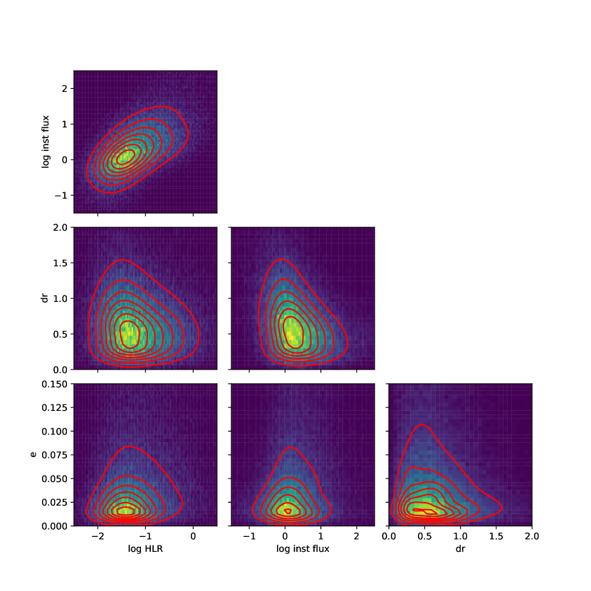
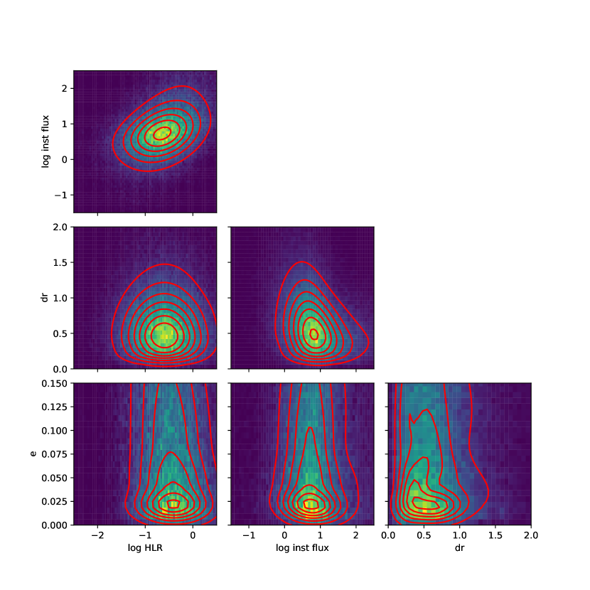
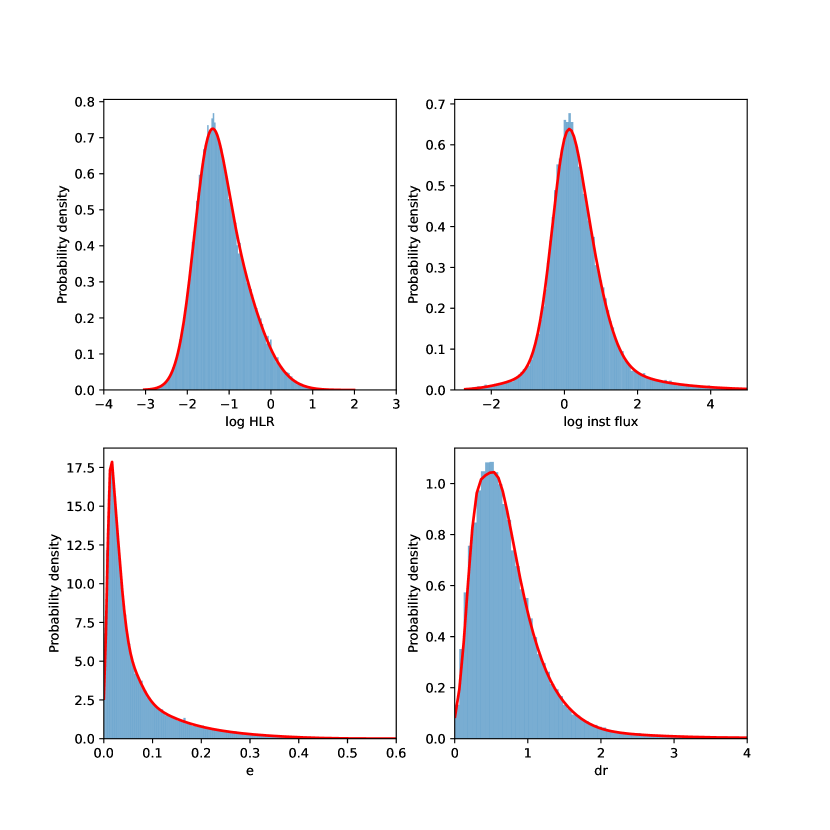
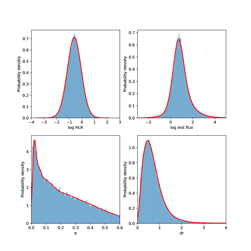
Because these distributions strongly correlate with galaxy morphology in the CosmoDC2 catalog, we perform separate fits for bulges and disks. The number of Gaussian components in each fit, 36 for bulges and 28 for disks, was chosen to maximize the evidence lower bound (ELBO) score for each model. All fits were run to convergence, defined as an expectation-maximization iteration with a lower bound average gain on the likelihood (of the training data with respect to the model) below 0.001. Each Gaussian component has an independent covariance matrix. A small regularization value of 1e-6 was added to the diagonal elements of each covariance matrix to ensure they would all be positive at every computational step. Figures 1 through 4 show various marginal projections of the full four-dimensional BGMMs (the contours and density curves plotted in red), compared to the true data distributions (the histograms).
By likelihood, we mean the probability that a given galaxy light profile will produce a specific image in a given telescope exposure. By a galaxy’s light profile, we mean the time-averaged distribution of galactic light hitting the top of Earth’s atmosphere. The same light profile will randomly produce different telescope images due to factors such as sky noise, photon shot noise, and PSF fluctuations. We model the likelihood by assuming that the intensity of each coadd image pixel is Gaussian-distributed and statistically independent of all other pixels, using a variance level estimated separately for each pixel by the Pipelines. For a given assumed galaxy light profile, we take the mean of each pixel’s likelihood distribution to be the convolution of that profile with the coadd PSF, integrated over that pixel. This is equivalent to simulating a noiseless image of the galaxy after convolving it by the PSF, all of which we do using GalSim (within JIF, described below). For such image simulations we use a Kolmogorov PSF, as defined in GalSim, with an FWHM of 0.77″. The specific FWHM used here was tuned to yield accurate mean posterior estimates of galaxy ellipticity for an exceptionally bright, signal-(as opposed to noise-)dominated, disk-shaped galaxy. Similar to our choice of prior, this choice of PSF width gives us a semi-idealized probabilistic model with which to study the maximal accuracy that can in principal be attained for this Bayesian approach.
4.2 Realistic and Simplified Data Sets
Even though we have taken steps to construct such an idealized model corresponding in many ways to the true prior distribution of galaxy parameters and to the true properties of the data-generating processes (i.e. the likelihood), there remain significant differences between our assumed probabilistic model and these true processes. In reality, even for the DC2 data set, the PSF is generally more complex than the simple isotropic Kolmogorov form, its FWHM varies within and between images, and it can change discontinuously within an image for coadds constructed via the present Pipelines, so a single “true” PSF width or even a single analytic form will never exactly match the true PSF that yielded our data. The variance plane adopted for our likelihood model is just that estimated by the Pipelines, and so in general will not exactly match the true variance of the true data-generating process. The photometric calibrations are estimated via a linear fit and so will not exactly match the true pixel intensity response for similar reasons. Furthermore, the photometric calibrations are assumed to be constant within and between images, whereas in reality these can vary. The single-component Sérsic profiles we assume for each galaxy do not exactly correspond to the bulge-plus-disk-plus-knots profiles that were actually used in the DC2 image simulations. Coaddition introduces covariance between pixels that we have completely ignored in our likelihood model. Optical artifacts such as ghost images, electronic artifacts such as the brighter-fatter effect (Guyonnet et al., 2015), and other technical features of real data have no place at all in our present model.
One therefore anticipates some level of mismatch, on average, between the truth and the estimated posteriors under our model, even for this simulated DC2 data set. To see the specific impact of these simplifying modeling assumptions, we generated a second, “simplified” data set with the same distribution of true galaxy properties as the main DC2 data used for this analysis, but with images of those galaxies constructed in GalSim in a manner that precisely matches our modeling assumptions, including the form of the PSF, the assumed variance plane, the photometric calibrations, and a pure bulge or disk morphology for every galaxy. By way of contrast, we refer to the DC2 images as the “realistic” data set. We then ran essentially the same MCMC fitting procedure on both data sets; the following section describes the one difference.
4.3 Conditioning on Selection
The Pipelines detection algorithm convolves an image by a Gaussian approximation of the PSF, and then identifies pixels in the convolved image that sit above a minimal threshold. This threshold is computed separately for each coadded patch and represents a level of PSF-matched pixel intensity five times the estimated noise level (“”). The corresponding maximum-likelihood total flux of a PSF-shaped light source is given by this threshold divided by the effective area of the PSF, defined by where is the integral of the PSF over a pixel displaced by from the center of convolution (Bosch et al., 2018). This defines a total flux level for an astronomical object with a point-source morphology. The specific level in a given patch corresponds (for the photometric calibrations given in Appendix A) to an -band AB magnitude (mag) of 25.5 on average, plus or minus 0.1 depending on the patch. The actual amount of light collected in the pixels around a specific object varies between exposures, so roughly speaking, half the time a object will produce enough light to be detected, and half the time it will not. Thus, the footprints in the realistic data set only include images of objects containing more than the average amount of flux such objects are expected to produce. This significantly skews the average likelihood of the image pixel data for these objects if no correction is applied.
In Bayesian terms, we must condition the posterior, and hence the likelihood and prior, on the fact that the footprints must pass a set of selection criteria to be considered for analysis. This condition varies significantly between the realistic and simplified data sets for galaxies near or below the total flux threshold. All the simulated data images in the simplified data set are fit regardless of whether they would be bright enough to pass the Pipelines detection algorithm, or how many detection peaks they might have, and only one true underlying object is used to simulate the light in each image. In other words, no special selections have been applied to the simplified data, so its probability of appearance is not conditioned on any special assumptions. Therefore, the assumed probability of any given image pixel containing a given amount of instrumental flux exactly matches the likelihood model described in section 4.1.
In contrast, the realistic data examples must pass three significant criteria to be selected for analysis. The pixel values must be such that they pass the Pipelines detection algorithm, which broadly means that the observed instrumental flux must be some combination of very bright and sufficiently PSF-like. Having passed the detection process, the pixel data becomes a footprint. Recall that we additionally restrict our attention to so-called isolated footprints, which introduces two additional selection criteria. The first is that, among the true objects the footprint pixels overlap, one of those true objects must have a flux at least 50 times larger than the total flux of all the others. The second is that the footprint must have exactly one peak.
These selection criteria mean that the likelihood for the realistic data must be conditioned on the fact of selection. Formally, for any given data example,
| (4) |
where is the six-dimensional parameter vector describing the true properties of the underlying galaxy, is the observed array of specific image pixel values, and is the condition that this data example has passed a specific set of selection criteria. Since directly determines the set of true values considered in this study, the conditional prior should reflect that fact for both the simplified and the realistic data sets. This is precisely the prior described in section 4.1, constructed by fitting a smooth density function (specifically a BGMM) to the set of true values underlying our footprint sample. Once is specified, the condition does not influence in the simplified data set, because any rendered is analyzed for every example. The conditional likelihood therefore reduces to , which is just the likelihood as described above (i.e. independent Gaussian-distributed pixel values). However, in the realistic data set, the fact of detection deeply influences above and beyond the value of . For example, some specific pixel arrays will pass the Pipelines detection algorithm and some will not, which just depends on the choice of detection algorithm, which is totally independent of whether is more or less likely to be produced by a galaxy with a given .
By making the approximations described in Appendix B, we can write the selection-conditioned likelihood as
| (5) |
The denominator is the total probability that a galaxy with true parameters would be observed with any image pixel array passing the Pipelines detection algorithm. We can place an approximate lower bound on this integral by computing the probability that the pixel in the detection image (the original image convolved with a Gaussian approximation of the PSF) covering the galaxy’s center would be bright enough to pass the threshold. Since the likelihood is assumed to be Gaussian and independent in every image pixel, the -convolved image has a Gaussian distribution in every pixel as well. Its mean is given by the value of the central pixel in a -convolved image of the mean galaxy light profile, which we compute by taking the galaxy image used for likelihood calculations (simulated in GalSim by convolving an elliptical bulge or disk model with a Kolmogorov PSF) and convolving it with the same used by the Pipelines for detection. The variance is given by the central pixel of a convolution of the variance plane with squared.111111For a constant variance plane, which is often approximately the case, this is just equal to the variance in any one pixel multiplied by the effective area of the PSF. Nevertheless, for the sake of rigor we compute the exact convolution each time. The integral goes from the minimal detection threshold (for which we use the value established by the Pipelines in every patch) to infinity, which means we are computing a complementary error function, i.e. 1 minus the cumulative distribution function of the Gaussian distribution with the above mean and variance. We compute this using the implementation of this function in scipy.stats.
Since the integral is the probability that any image produced by would pass the Pipelines detection algorithm (but not necessarily any other selection criteria), another lower bound on this integral is the probability that any image produced by would pass all three selection criteria. We estimate this probability empirically by finding, within various bins of flux, the fraction of galaxies with flux in a given bin that ultimately give rise to a footprint passing all the selection criteria. Our final estimate for is the maximum of the two lower bound estimates described above. The likelihoods we compute for the realistic data set are selection-conditioned by taking the unconditioned likelihood and dividing it by this estimate for the integral.121212Because we only ever need to compute the log-likelihood, we actually just take the log-unconditioned-likelihood and subtract the log of the estimated integral.
5 MCMC
The functions for computing the prior and likelihood are implemented in JIF, an open-source131313github.com/mdschneider/JIF Python framework for organizing these computations for astronomical images and running MCMC. JIF stands for Joint Image Framework, emphasizing that a single object may have multiple distinct images taken of it, all of which likelihoods the framework can model jointly, enabling maximally constraining posterior inference. The user must supply a prior function, along with certain items needed for the likelihood (all of which can be different for each separate exposure) such as the telescope image, a description of its WCS, PSF, estimated background (if nonzero), and variance plane, and a mask specifying which pixels are to be modeled; JIF then handles the rest. For each galaxy modeled in this study we use only a single image taken in one photometric band by one simulated telescope, but multiple exposures, bands and/or telescopes could be jointly modeled in future work, restricted only by available computing time and by user knowledge of each image source.
Given the above prior and likelihood model, we use JIF to estimate the corresponding posterior for each footprint with an affine-invariant ensemble MCMC method described in Goodman & Weare (2010) (hereafter G&W), as implemented in emcee (Foreman-Mackey et al., 2013). This has the practical advantage of requiring relatively little parameter tuning. The chains consist of sequences of six-dimensional vectors that model the six parameters of interest of the galaxy contained in a given footprint. Rather than a single sequence for each footprint, a chain in the G&W method comprises some number of parallel sequences or “walkers,” which we set to be 16. In principle this number could be tuned to accelerate convergence or to improve the statistical quality of the converged chains, but we selected 16 simply because it yielded consistently convergent chains in early experiments and has continued to do so. The chains progress via “walk moves” as defined by G&W, using the full walker complement to estimate the covariance matrix for each proposal.
Properties of the posterior are estimated from corresponding sample properties of the chains. The parameter vectors sampled by each walker do not necessarily adhere well to properties of the posterior at the start of sampling, but in general the walkers make more reliable draws from the true posterior distribution as they progress. Hence, often the posterior can be estimated more accurately by ignoring some number of initial steps in the chain, a procedure called “burn-in.” All MCMC runs reported in this study consist of 1,000 burn-in steps followed by 3,000 posterior inference steps. In initial tests with a handful of diverse footprints, these numbers of steps consistently yielded highly stable estimates of the posterior that don’t significantly change when the chain is re-run or when the number of steps is increased. These features suggest robust convergence, which is also indicated by the results shown in Section 6.
To avoid a lengthier burn-in phase as well as potentially pathological (and highly unrealistic) regions of parameter space for which GalSim cannot render images, we start each chain at parameter values near a maximum a posteriori (MAP) estimate of those parameters. We use the L-BFGS-B algorithm (Byrd et al., 1995) implemented in scipy.optimize to iteratively sample parameter values, moving in the direction of higher likelihood times prior, until no significant improvement is possible, at which point one has an estimate of the MAP parameters. Occasionally the L-BFGS-B algorithm fails for one reason or another, in which event we retry the fit with the SLSQP algorithm (Kraft, 1988); one or the other of these nearly always succeeds. Each of the 16 chains starts at an independently-sampled point in parameter space, with each parameter separately sampled from a Gaussian distribution with a mean equal to its estimated MAP value and a standard deviation of one percent of that value—in other words, every chain starts off within about one percent of the MAP values. To initialize the MAP fit, both ellipticity components are set to 0, the centroid position is set to the location of the footprint’s detection peak, and the flux to the sum of the footprint’s pixel intensities; the half-light radius is set to its expected value (conditioned on the aforementioned flux estimate) under a greatly simplified “prior” consisting of a two-dimensional Gaussian fit of the true distributions of flux and half-light radius141414More precisely, their natural logs. of galaxies in our data set, using separate fits for bulges and disks as in our full prior. In the few hundred instances of failed MAP fits, we initialize the chains using these rougher estimates.
Each of these steps—a first rough initialization, followed by an MAP fit, followed by robust MCMC—requires increasing amounts of time but offers increasing accuracy and insight. The first step can be done almost instantly, but its estimates have only a loose relationship to either the posterior distribution we are trying to estimate. It might perform just as well as an MAP fit to initialize the MCMC chains (1,000 burn-in steps does a good job of getting a chain to converge starting from just about anywhere), but we went with the latter because it is by definition in the part of parameter space that a well-converged chain should sample from most often, and in any case it does not extend the total compute time by a significant fraction. The MAP fit generally requires at most a few hundred simulated likelihood and prior computations per footprint. MCMC, as implemented by JIF using emcee, takes several minutes per footprint on a modern commodity laptop or high-performance computing node, and is by far the most computationally expensive step per footprint performed in this study. For 16 parallel chains with 4,000 steps each, it requires 64,000 total likelihood and prior computations.151515Technically, for both the MAP fit and MCMC, we only directly evaluate the log-likelihood and log-prior, which are significantly easier to compute than their exponents. For this study we fit 149,933 total footprints, requiring more than 8,000 CPU hours for the MCMC alone, which ultimately rendered 9.6 billion simulated galaxy images. Because we model each footprint independently, the MCMC run for each footprint can be computed in parallel, so the actual wall clock time depends on how many parallel computing nodes one has access to. Using 1,728 parallel cores at Lawrence Livermore National Laboratory (LLNL), the entire suite of MCMC computations was completed in under six hours. The preceding numbers apply to the realistic data set on its own; analysis of the additional simplified data set required similar compute.
Of the footprints we fit, we gathered the complete catalog truth information for 134,311. This includes everything that lies inside both tract 3820 and one of CosmoDC2 HEALPixels 9685, 9813, or 9814, which together comprise a contiguous region of space covering most of the tract. The summary plots in Section 6 reflect this set of footprints. Of the 268,622 corresponding chains we analyze (one each for the realistic and simplified versions of every footprint), all but three ran to completion without errors. The success rate is not always this high for all possible priors and chain initialization methods. In a sample of a couple dozen footprints on which we tested a completely uniform prior, we observed numerous failed fits stemming from highly unrealistic parameter samples that result in GalSim rendering errors, and the chains that ran to completion were often rather low-quality estimators of the posterior. This seems to be the underlying source of the large number of fit failures reported in the ProFit analysis by Robotham et al. (2017): as is typical among studies introducing Bayesian galaxy modeling codes, Robotham et al. (2017) describe their likelihood model in detail, but do not describe the assumptions on their prior, presumably indicating an implicit uniform prior. Such a prior was in fact justified in their study because their simulated data set was generated from a uniform distribution of model parameters. However, they encountered the predictable result of a likelihood-dominated posterior, which is an increasing number of fit failures, stemming from implausibly extreme parameter estimates, as the galaxy S/N decreases. For any similar efforts going forward, we therefore strongly advocate using an informed prior of the sort adopted for this study, for practical reasons of chain convergence in addition to the statistical properties illustrated below. The use of a substantially informed prior is additionally justified by the fact that we do, in fact, have substantial prior knowledge of what is reasonable to expect, stemming from all previous and ongoing telescope surveys. By incorporating as much of this knowledge as possible in the prior, we obtain posteriors that are both maximally constraining and most accurately representative of our actual level of uncertainty.
6 Results
As described in Section 4.2, our footprint data set consists of two basic types, realistic and simplified, each of which has two possible true light profiles, bulge or disk, for a total of four distinct variations that we analyze independently. Each of the six model parameters, in each of the variations, has a marginal posterior distribution worth examining. We should also examine the statistical reliability and general properties of the chains according to various metrics, which again all vary for each parameter and data variation. There are hence a prodigious number of possible plots of interest. In this section we highlight a subset of results that give a sufficient basis for discussion. Recall that we fit the true bulges (more precisely, the galaxies that are more bulge-like than disk-like) with a pure bulge light profile, and use a BGMM prior that has been fit to the true distribution of bulge-like galaxy properties in our data set; disks are fit with a corresponding disk light profile and prior. In a real-world analysis, for which the galaxy morphology is unknown ahead of time, the parametric light model and the prior would need to support multiple distinct morphological possibilities, but we have not developed that apparatus here.
6.1 Chains
Figure 5 shows several views on the progress of the log-half-light radius values of a single chain, consisting of 16 parallel walkers iterating for 4,000 steps each. The top plot shows the trace of each separate walker’s half-light radius value at every step. The individual traces exhibit so much random variability that it can be difficult to discern meaningful trends, but this plot shows that the gross behavior of the walkers does not change noticeably over the course of the chain except for a relatively small fraction of initial steps in the burn-in phase. The middle plot shows the mean of each walker’s complete trace up to each step. This plot makes apparent that the walkers in this example start out at a lower value than what they end up at, steadily gravitate toward their final resting place over the course of a few hundred steps, and then settle in to an extended phase of steady behavior, during which the means of each separate walker gradually converge. The bottom plot shows the overall mean of the combined values of all walkers, together with the spread from the 16th to the 84th percentile of all walker values, up to each step. Here we have not omitted any burn-in steps from consideration when evaluating means and spreads. The form of this plot looks quite similar if we treat the initial 25% of steps up to any given point as burn-in, suggesting that we might be able to decrease the number of burn-in steps without significantly changing the chain’s statistical characteristics.
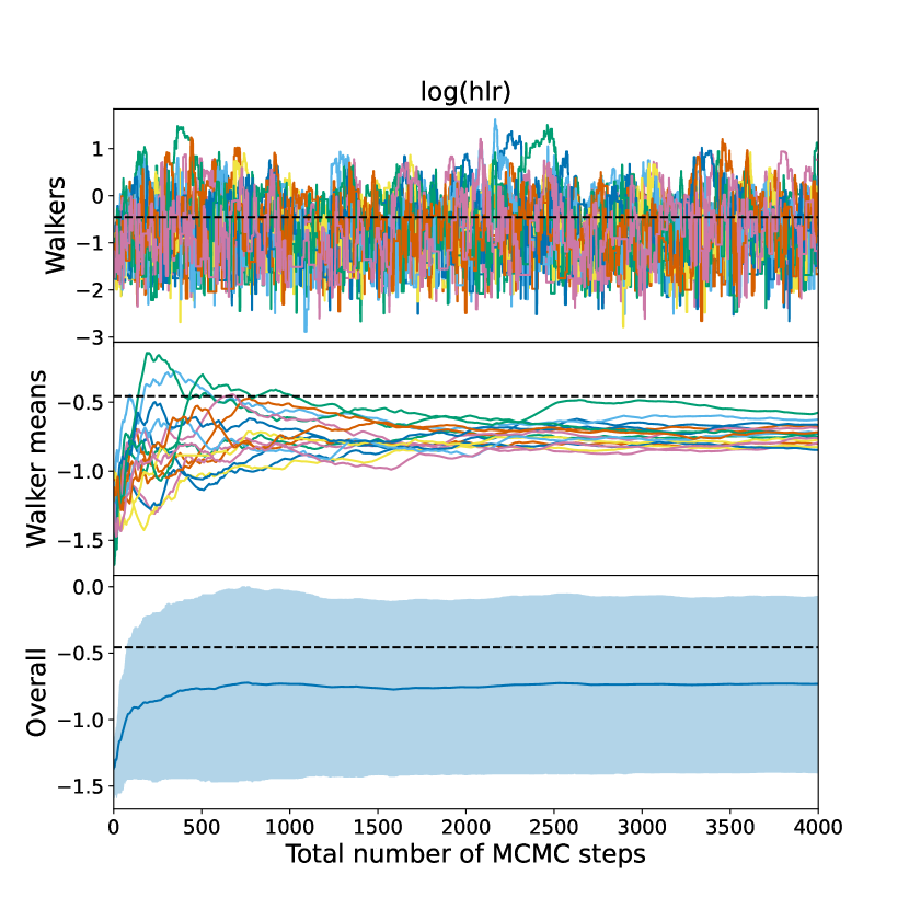
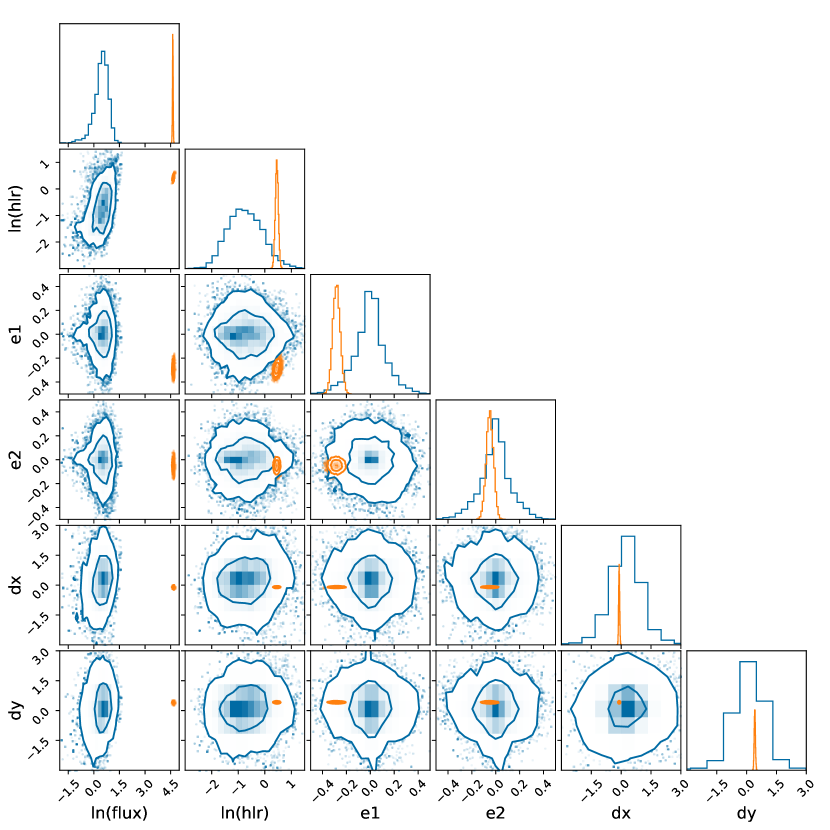
Figure 6 illustrates the six-dimensional posteriors for two different examples: one with a mean flux close to the detection threshold, for which the prior largely determines the posterior, and one with a flux bright enough for all marginal posteriors to be predominantly likelihood-constrained (see the discussion in Section 6.3 below). For this and all other figures showing final posterior estimates, burn-in steps have been removed. As expected, the posterior widths decrease as the amount of signal increases. The relative amount of decrease depends on the parameter: the dx–dy contours shrink almost to a point, whereas the e1–e2 contours remain clearly spread out, indicating that e1 and e2 require more signal to infer compared to dx and dy. The true parameter values for each example lie inside one or both of the 2D contours in all cases. This does not always need to happen for the posteriors to have their nominal coverage—we expect that the 95% contours should not contain the truth 5% of the time—but it is certainly nice if the 95% contours contain the truth more often than not. We explore the posterior calibration more systematically in Section 6.3.
6.2 Chain properties
Figures 7(a) and (b) show the distributions of times needed for chain inference in the simplified data set of bulge galaxies (any distributions noted in this section are largely similar for all data variations). Finding the MAP parameters, with which the chains are initialized, takes between 1 and 2 seconds on average, while 4,000 MCMC steps with 16 parallel chains takes between 3 and 4 minutes on average on a high performance computing cluster at LLNL. Similar run times are obtained for a handful of test examples on a modern commodity laptop. These run times compare favorably with pysersic, which takes “a few minutes or less on modern laptops” to fit a 7-parameter Sérsic profile (Pasha & Miller, 2023); AstroPhot, which took 738.5 seconds to sample a 13-parameter model of various components in a scene (Stone et al., 2023); and BANG, which needed about 30 minutes per galaxy to fit three different morphological models with 14 to 18 parameters each (Rigamonti et al., 2023). We stress that none of these comparisons are absolute because each analysis used a distinct computer architecture, modeled a distinct parameter set, and made a distinct determination of the number of MCMC samples necessary for statistical confidence in the results. Nevertheless, it is noteworthy that the single-model run times for all of these approaches ended up in the same ballpark.
Various metrics have been developed in the MCMC literature to gauge the convergence of chains. One popular metric is the Gelman–Rubin statistic, as defined in Gelman & Rubin (1992). Figure 7(c) shows the distribution of Gelman–Rubin values for log-HLR in simplified bulge footprints. Most values lie between 0.99 and 1.01. Each parameter has its own value for this statistic, though we find that the distributions for every parameter look quite similar. The interpretation of this statistic is muddied when using correlated parallel chains as we do here, so Foreman-Mackey et al. (2013) instead define a measure of the integrated autocorrelation time, which counts the average number of chain steps needed to generate a statistically independent sample from the posterior. Figure 7(d) shows the distribution of integrated autocorrelation times for log-HLR. As before, the distributions of this value for all parameters are all similar. Since we use 3,000 MCMC steps for posterior estimation after burn-in, and the integrated autocorrelation time is almost always less than 30 steps, we conclude that more than 100 fully independent posterior samples were drawn for each parameter in nearly every footprint.
6.3 Comparison to truth
Figure 8(a) shows the difference between the posterior mean and the true value of the natural logarithm of the total instrumental flux. In this and all other plots with marginal distributions, the marginal curves in each bin are normalized to have the same total area under the curve, in order to highlight their shapes. As shown both in the even distribution of points and in the well-centered marginal curves, galaxies brighter than mag 26 (log-flux greater than about 1) have virtually unbiased posterior means, when averaged over many different galaxies. Individual galaxies can still have posterior means different from the truth, though the average amount of difference decreases as the sources get brighter. Figure 8(b) compares the posterior directly to the truth, this time showing the 68% inner credible for each posterior. Just as the posterior means adhere more closely to the truth as the true galaxy brightness increases, so too do the credible intervals shrink with increasing brightness. This tendency is illustrated more comprehensively in Figure 9(a), which shows how the credible intervals of any given percentage width shrink as the brightness of the underlying galaxy increases.
Even as the intervals shrink, they continue to overlap the truth the expected fraction of the time, as illustrated in Figure 9(b). The latter figure is the most direct illustration of the reliability of a probabilistic interpretation of the MCMC-estimated posteriors, as it shows how often the credible intervals of various widths overlap the truth. If the estimated posteriors are reliable, then a specific -percent interval should overlap the truth percent of the time, on average over many galaxies, resulting in a perfectly diagonal plot. We see that this broadly holds to within statistical errors for much of our data, except for the dimmest galaxies. The light blue curve, corresponding to galaxies dimmer than mag 27, shows the greatest discrepancy. The direct cause of this discrepancy is clear from either of the two preceding figures: the MCMC-estimated log-flux is systematically higher than the true flux for these dim galaxies.
More specifically, as shown in Figure 8(b), the estimated posterior for log-flux is basically constant for all galaxies dimmer than mag 27. This is because the observed pixel data for such galaxies provides essentially no information about the underlying galaxy. The minimum detection threshold is brighter than mag 26 in every patch, meaning that the dimmest galaxies only enter our data set if their DC2 images coincided with random noise fluctuations that just happened to rise above the detection threshold. Once selection corrections have been taken into account, the likelihood of observing any given footprint image in our realistic data set is essentially independent of the underlying galaxy brightness for galaxies dimmer than mag 27. The simplified data set was constructed by taking the mean light profile for each galaxy and randomly generating an amount of noise around that profile consistent with the variance plane, and for the galaxies below the detection threshold, the typical amount of noise far outstrips the mean signal. In this case there are no selection corrections, but the likelihood is still insensitive to variations in the underlying galaxy flux for the dimmest galaxies.
This insensitivity can be intuited by considering the likelihood for the image flux in one pixel, a Gaussian distribution with mean and standard deviation . The probability density function (pdf) of observing a pixel value is proportional to . Taylor expanding around , we get an overall factor of times the series
| (6) |
When is much less than , a many- variation in is required to shift the series away from 1 by a noticeable amount. Thus the pdf can be characterized by “ plus a small perturbation” for most of the values likely to be produced from this light source. Since the maximum likelihood estimate of just equals , the peak of the likelihood as a function of is typically within of 0 for such galaxies. The width of the likelihood as a function of is characterized by the derivatives of the pdf with respect to . For , all of the derivatives are equal to a constant (with respect to ) plus terms of order , so the first few derivatives do not have any significant -dependence. Thus, as long as , the likelihood has a very consistent peak and width as a function of for most of the values likely to be produced.
Since the posterior is proportional to the likelihood times the prior, and since the shape of the likelihood is highly consistent for any data likely to be produced from the dimmest galaxies, the posterior becomes largely independent of the data for such galaxies. The flux level at which this occurs in our data is illustrated by the flat section of the curves on the right side of Figure 9(a), as well as by the flattening of the left section of Figure 8(b), which in turn translates to the diagonal “swoosh” on the left section of Figure 8(a). Reasonable values of definitively exclude very high values of on the basis of the likelihood alone, but for values closer to 0 the likelihood has a broader base of support and the posterior is more strongly shaped by the prior. The flux level where our posteriors separate from the truth and become constant corresponds to this regime. The fact that the constant posteriors are shifted upward from the truth in the dim-galaxy regime corresponds to the fact that our prior is strongly peaked at mag 26, which also explains why these posteriors are centered close to mag 26 (log-flux just under 1) in Figure 8(b). Since the posterior for almost every galaxy in this flux regime has almost exactly the same too-high mean and the same width, irrespective of the true galaxy brightness, the credible intervals of various sizes consistently sit above where they need to be, resulting in the pronounced undercoverage illustrated by the light blue curve in Figure 9(b).
Figure 9(a) shows a common feature of the interval size plots: as the true galaxy brightness increases, the posterior intervals shift from a steady, flat mag-dependence in the high-mag range, to a region of rapid shrinking in the mid-mag range, followed by continued shrinking and convergence in the low-mag range. Figures 10(a),(b) illustrate this tendency in two other parameters of interest, the half-light radius and the first component of ellipticity. These figures show that estimating a parameter from data can require different amounts of galaxy brightness, depending on the parameter. Overall flux takes relatively little galaxy brightness to begin to infer reliably, half-light radius requires a bit more brightness to infer, and ellipticity still more. The ellipticity intervals increase somewhat in the transition region between high-mag and mid-mag, before collapsing rapidly at lower mags. This seems to be caused by the fact that the ellipticity prior is markedly wider in the middle-flux range, as shown by the mountainous shape of the e vs. log inst flux distribution in Figure 1. The flat portion of plots such as Figures 10(a),(b) reveals the galaxy brightness regime over which the parameter inference is effectively independent of the truth, which causes the mean and widths of the resulting posteriors to exhibit the same steadiness, irrespective of truth, exhibited by the lowest-flux galaxies in Figure 8(b). Figures 10(c),(d) show corresponding behavior for posterior credible intervals of the half-light radius and the first component of ellipticity.
6.4 Comparison between data sets
Figures 11(a),(b) show distributions of interest for log-flux in the simplified disk-only, as opposed to the bulge-only, data set. The posterior calibration is generally better across all parameters for the disks than for the bulges. The disk plots just look like slightly tweaked versions of the bulge plots, with better calibration and generally somewhat tighter intervals. The two tendencies seem to be related, in that the disk model can evidently constrain the parameters of interest of disk galaxies with less signal (i.e. galaxy brightness) than the bulge model needs for bulge galaxies, and all parameters show a tendency to adhere to truth better (for at least the simplified data set) when the posterior has been conditioned on a greater signal. For brevity’s sake we don’t show all the disk plots here—the point of the present study is not to gain an exquisite understanding of CosmoDC2 bulges and disks, but rather to establish the general capabilities and limitations of our MCMC method for posterior inference of galaxy properties.
The realistic data set results are mostly quite similar to those of the simplified data set, with some stand-out differences. Figure 12(a) shows perhaps the most concerning difference: a pronounced upward bias in the estimated flux for the brightest galaxies. This bias results in an undercoverage of the flux posteriors for bright galaxies as illustrated in Figure 12(b). The calibration improves if we apply a post-hoc bias correction—essentially, the flux posteriors are about as wide as they should be, just too high. The origin of this bias is a mystery. It shouldn’t be due to our photometric calibrations, because those were derived from a direct comparison of instrumental flux to true expected flux in the brightest galaxies (see Appendix A). Since the likelihood most strongly constrains the posterior for the brightest galaxies, this may reveal a problem with our likelihood model’s ability to describe realistic data. More work will be needed to clarify the true causes, which may include the fact that we do not model correlated variation between image pixel values introduced by the coaddition process, or the fact that we use a consistent, perfectly isotropic PSF across all examples. We attribute the downward shift in the posterior mean for the lowest flux galaxies, compared to the simplified data set (Figure 8a), to the selection corrections (Section 4.3), which give added weight in the likelihood to flux levels below the detection threshold. The size of this downward shift illustrates the significant impact of applying these selection corrections when modeling low S/N galaxies. The convergence of the low-flux posterior means toward the truth, and the improvement in calibration shown by the light blue curve in Figure 12(b), demonstrate the utility of applying these corrections and validate the approximations described in Section 4.3.
Figures 13(a) and (b) show corresponding plots for the half-light radius. Like flux, the posterior mean for half-light radius exhibits a consistent upward bias for the brightest galaxies, although the brightness threshold at which this bias becomes apparent is higher for half-light radius than for flux. The overwhelming majority of galaxies in the brightest mag bin do not exhibit a systematic mean half-light radius bias, as shown by the dark blue marginal curve on the y-axis in Figure 13(a). Nevertheless, the calibration for the highest flux galaxies exhibits a consistent level of under-coverage (Figure 13b), suggesting that the posterior widths are too small by a consistent factor. The posterior distributions for the first component of ellipticity, shown in Figure 14(a), look similar to those of the simplified data set (Figure 10d), as does the calibration (Figure 14b).
7 Conclusions and Outlook
We have developed a framework for MCMC inference of posterior distributions of galaxy properties in LSST images, and tested it on well-isolated galaxies detected in -band coadds from the DC2 simulations. Our analysis of 149,933 detection footprints from realistic images establishes that the current JIF framework can be used for large parallel computing runs and can handle most examples of data seen in practice without catastrophic errors. Stone et al. (2023) contend that “it is common for the statistical [MCMC] uncertainties to underestimate the true uncertainty, especially for fits to real data where the fitted models (i.e., Sérsic) are only approximations to the true shape of a galaxy.” That claim is motivated by the demonstration of a single simulated example with a posterior that fails to cover the truth within its 95% credible intervals. Here we have tested this claim more rigorously by looking at the average posterior calibration across more than galaxies. Our plots in Section 6 show that, with properly informative priors, a sufficiently well-constructed likelihood, an assumed Sérsic model at least broadly similar to the true light profile, and sufficiently long and well-converged MCMC chains, we can in many cases establish good probabilistic calibration. The posterior intervals can be treated as reliable estimates of uncertainty, across galaxy types and parameter combinations, for at least those galaxies which are bright enough to be detectable on average and which do not exhibit systematic biases in their posteriors as noted above.
From the observed degradation of results for high-flux galaxies when going from simplified to realistic data, we deduce that our posteriors would benefit from further refinement of the assumed likelihood model. The likelihood is governed in particular by the assumed variance model and the assumed PSF. The PSF has nontrivial shape and size uncertainty that we have not tried to model here, but we have designed JIF to straightforwardly accommodate such uncertainty, which could be modeled in future work by introducing a few extra fit parameters. The coaddition process, in which the pixel values of various single exposures are warped to fit a common sky coordinate grid and then stacked on top of each other, introduces covariance between pixels in the resulting image plane, along with PSF warping and discontinuities in the PSF at the boundaries of constituent single exposures, none of which we model here. Some of the posterior bias and coverage issues we see in this study may stem from these difficulties, and could be corrected for by more detailed likelihood modeling that includes an estimate of pixel covariance, by switching to a different coaddition procedure, or by modeling all the individual constituent exposures instead of coadds, as was done in the application of LensFit to Canada–France–Hawaii Telescope data (Miller et al., 2013).
The latter approach would in principle yield the most constraining posteriors since it doesn’t “throw away data,” but it multiplies the computational burdern, since each separate exposure must be simulated when computing the likelihood. That is the chief reason we have not attempted to model all six LSST filter bands in the present study, as that is effectively equivalent to simulating six times as many images in each likelihood computation. Future work will seek to model these extra bands in order to take advantage of all the data at our disposal. This would additionally allow us to model the redshift, which we could describe parametrically by assuming that the spectral energy density (SED) for a given galaxy is the probability-weighted sum of a few template SEDs, with a specified redshift dependence. The weak lensing potential could be constrained by simultaneously modeling multiple galaxy profiles in conjunction with a potential model, the ultimate goal of JIF.
Another possible source of error in the posterior may be model bias, because our single-component bulge or disk profiles do not exactly match the bulge-plus-disk-plus-knots profiles that were actually used to produce the DC2 images. Since the assumed light profile is used to compute the likelihood, this again impacts the brightest galaxies in particular. This model bias could be mitigated by replacing the single-component profiles with a bulge-plus-disk profile in JIF (to be closer to the DC2 truth), or a more complex profile accommodating more realistic shapes, as long as that profile is parametric. The specific MCMC algorithm used here does not evaluate the model evidence (the integral of likelihood times prior over all valid parameter combinations). However, if desired, a postprocessing tool such as Harmonic (McEwen et al., 2022) could be applied to the emcee chains to estimate the evidence, and various other MCMC implementations evaluate it directly. As noted in Bridle et al. (2001), the model evidence balances goodness of fit with the number of degrees of freedom, providing a tool for selecting a preferred galaxy light profile model from various competing possibilities. This is an intrinsic advantage of Bayesian methods, and a natural subject for future study. Alternatively, we can consider replacing our Gaussian-distributed likelihood model with a Student-T distribution, which Robotham et al. (2017) advocate as a way of regularizing simple Sérsic fits of high S/N galaxies with significantly non-Sérsic light distributions.
The Bayesian approach hinges crucially on the choice of prior, particularly for low-flux footprints, for which the likelihood has little constraining power. This issue is especially acute as the dimmest footprints will be the most numerous in our data. Furthermore, these are exactly the galaxies which are generally to be detected for the first time by LSST, making it difficult to rigorously establish a prior model for their distribution. Nevertheless, precursor telescope surveys, though they record a substantially smaller fraction of the sky at equivalent or greater depth compared to LSST, still give us some direct empirical sense of the distribution of dim galaxies, which we can use to shape our prior. This was the approach used to the construct the CosmoDC2 simulation, which was verified against the surveys noted in Section 2; in the future, deeper and more extensive data from other surveys can be used. This data can form the fitting target of a generative model that serves as a prior. Here we have used a BGMM as such a model; other popular approaches such as variational autoencoders (Kingma, 2019) or normalizing flows (Kobyzev et al., 2021) could be examined in the future. In any case, we stress that the posterior samples obtained here on individual galaxy parameters serve as strictly provisional, “interim” posteriors when following the full hierarchical inference strategy of S15 for constraining cosmological parameters. From this standpoint, the most essential requirements on the single-galaxy fits are that the MCMC chains converge and run for long enough to thoroughly sample the interim posterior. As we discuss in Section 5, our MCMC chains nearly always run to completion using the prior adopted in this study, whereas a more uniform prior will routinely result in fit failures of the kind reported in Robotham et al. (2017), especially on low S/N galaxy images.
Initial experiments suggest that blended footprints can be handled reliably without any change to the fitting method beyond adding an additional light profile to the model, but this is ultimately a topic we have left for future study. Very roughly, doubling the number of galaxies in a footprint model would double the amount of time it takes to render each light profile (in the likelihood computation) and to compute the prior (once separately for each galaxy, though perhaps with some additional correlational structure). An -galaxy fit would require parameters to be jointly modeled under our current approach. The affine-invariant ensemble sampling strategies described in G&W do not require any separate tuning for separate parameters and should scale gracefully to such fits. The number of correlations between different parameters goes up as the square of the total number of parameters, so to robustly capture all these correlations it may be necessary to run the MCMC fit for more iterations, but this is hard to precisely determine ahead of actually running it and checking.
Our overall fitting approach requires a specific pixel array to fit, supplied by the footprints constructed by the LSST Science Pipelines in the present study, together with a specific number of galaxies to fit, supplied here by the the number of Pipelines detection peaks in each footprint. We have simplified our analysis of posterior reliability by limiting the scope of our study to cases in which the number of peaks corresponds exactly to the number of significant galaxies in every footprint. In reality, the total number of faint galaxies in any given patch of sky cannot be known with certainty because of noise. We could instead describe the number of galaxies probabilistically, in addition to the properties of each one, resulting in fully probabilistic catalog descriptions. This was done for crowded star fields by Feder et al. (2020) using MCMC and by Liu et al. (2023) using variational inference, but a comparable apparatus for galaxy catalogs has yet to be developed. One step in this direction was developed in Buchanan et al. (2022), which considered a variety of methods for probabilistically determining whether an LSST Science Pipelines footprint contains one or more than one galaxy above a given flux threshold, finding decent accuracy and calibration with a Gaussian process model. As described in that paper, such classification methods can readily be expanded to more general galaxy count estimators via a hierarchical series of ” vs. more than ” classifiers. Balancing one asserted number of galaxies against another can be done via the model evidence for different possibilities, as discussed for galaxy morphology above. Probabilistic catalogs would naturally incorporate our uncertainties about galaxy number counts into the uncertainties on cosmic shear obtained later in the S15 program. However, considering different numbers of galaxies adds to the computational burden of each fit.
Our method appears to be relatively fast compared to other published approaches. However, to place significant constraints on dark energy via weak lensing shear measurements, we will need to model a substantially larger portion of the sky than the 2.4 square degrees considered here. If exactly the present method is scaled up from 2.4 square degrees to 18,000 square degrees—the expected total sky coverage of LSST (Ivezić et al., 2019)—60 million CPU hours would be required. This would be a substantial, but feasible, computational burden for a high performance computing facility. Modeling all six filter bands would multiply this burden by an additional factor (probably less than six, since various steps of the MCMC computation remain unchanged as more bands/images are added), as would any of the other more detailed modeling proposals outlined above, including simultaneous modeling of blended galaxies. This motivates us to explore methods of reducing the run time. These could include optimizing the JIF and underlying emcee codes, using a better initialization method in order to reduce the number of burn-in steps, considering alternative MCMC approaches such as Hamiltonian Monte Carlo (used by pysersic and AstroPhot), refining our understanding of how many chain steps are actually needed per footprint to place constraints on dark energy, and potentially training a machine learning model to more quickly estimate the likelihood at each step. We are therefore optimistic that this approach can be extended to the full LSST data set. Our MCMC method could also be used to validate the outputs of a faster variational autoencoder or similar model for directly estimating the posterior on a subset of the LSST data, which would then increase confidence in the reliability of the faster model if it were then applied on the full data set.
References
- Abolfathi et al. (2021) Abolfathi, B., Alonso, D., Armstrong, R., et al. 2021, ApJS, 253, doi: 10.3847/1538-4365/abd62c
- Aihara et al. (2018) Aihara, H., Armstrong, R., Bickerton, S., et al. 2018, PASJ, 70, doi: 10.1093/pasj/psx081
- Albareti et al. (2017) Albareti, F., Prieto, C., Almeida, A., et al. 2017, ApJS, 233, doi: 10.3847/1538-4365/aa8992
- Bartelmann & Schneider (2001) Bartelmann, M., & Schneider, P. 2001, Phys. Rep., 340, doi: 10.1016/S0370-1573(00)00082-X
- Bertin & Arnouts (1996) Bertin, E., & Arnouts, S. 1996, A&AS, 117, doi: 10.1051/aas:1996164
- Blei & Jordan (2006) Blei, D., & Jordan, M. 2006, Bayesian Anal., 1, 121, doi: 10.1214/06-BA104
- Bosch et al. (2018) Bosch, J., Armstrong, R., Bickerton, S., et al. 2018, PASJ, 70, doi: 10.1093/pasj/psx080
- Bridle et al. (2001) Bridle, S., Kneib, J.-P., Bardeau, S., & Gull, S. 2001, in Proceedings of the Yale Cosmology Workshop, ‘The Shapes of Galaxies and Their Dark Matter Halos’ (World Scientific Press), doi: 10.1142/9789812778017_0006
- Bridle et al. (2013) Bridle, S. L., Kneib, J. P., & Bardeau, S. 2013, im2shape: Bayesian Galaxy Shape Estimation, Astrophysics Source Code Library, record ascl:1307.006. http://ascl.net/1307.006
- Buchanan et al. (2022) Buchanan, J., Schneider, M., Armstrong, R., et al. 2022, ApJ, 924, 94, doi: 10.3847/1538-4357/ac35ca
- Byrd et al. (1995) Byrd, R., Lu, P., Nocedal, J., & Zhu, C. 1995, SIAM J. Sci. Comput., 16, 1190, doi: 10.1137/0916069
- Capak et al. (2007) Capak, P., Aussel, H., Ajiki, M., et al. 2007, ApJS, 172, doi: 10.1086/519081
- Feder et al. (2020) Feder, R., Portillo, S., Daylan, T., & Finkbeiner, D. 2020, AJ, 159, 163, doi: 10.3847/1538-3881/ab74cf
- Foreman-Mackey et al. (2013) Foreman-Mackey, D., Hogg, D., Lang, D., & Goodman, J. 2013, PASP, 125, doi: 10.1086/670067
- Gelman & Rubin (1992) Gelman, A., & Rubin, D. 1992, Statist. Sci., 7, doi: 10.1214/ss/1177011136
- Goodman & Weare (2010) Goodman, J., & Weare, J. 2010, Comm. App. Math. and Comp. Sci., 5, doi: 10.2140/camcos.2010.5.65
- Guyonnet et al. (2015) Guyonnet, A., Astier, P., Antilogus, P., Regnault, N., & Doherty, P. 2015, å, 575, 17, doi: 10.1051/0004-6361/201424897
- Heitmann et al. (2019) Heitmann, K., Finkel, H., Pope, A., et al. 2019, ApJS, 245, doi: 10.3847/1538-4365/ab4da1
- Heymans et al. (2006) Heymans, C., Van Waerbeke, L., Bacon, D., et al. 2006, MNRAS, 368, doi: 10.1111/j.1365-2966.2006.10198.x
- Hirata & Seljak (2003) Hirata, C., & Seljak, U. 2003, MNRAS, 343, doi: 10.1046/j.1365-8711.2003.06683.x
- Ivezić et al. (2019) Ivezić, Ž., Kahn, S., Tyson, J. A., et al. 2019, ApJ, 873, doi: 10.3847/1538-4357/ab042c
- Kacprzak et al. (2014) Kacprzak, T., Bridle, S., Rowe, B., et al. 2014, MNRAS, 441, doi: 10.1093/mnras/stu588
- Kaiser et al. (1995) Kaiser, N., Squires, G., & Broadhurst, T. 1995, ApJ, 449, doi: 10.1086/176071
- Kilbinger (2015) Kilbinger, M. 2015, RPP, 78, doi: 10.1088/0034-4885/78/8/086901
- Kingma (2019) Kingma, D. 2019, Foundations and Trends in Machine Learning, 12, 307, doi: 10.1561/2200000056
- Kitching et al. (2008) Kitching, T., Miller, L., Heymans, C., van Waerbeke, L., & Heavens, A. 2008, MNRAS, 390, doi: 10.1111/j.1365-2966.2008.13628.x
- Kobyzev et al. (2021) Kobyzev, I., Prince, S., & Brubaker, M. 2021, IEEE Transactions on Pattern Analysis and Machine Intelligence, 43, 3964, doi: 10.1109/TPAMI.2020.2992934
- Komatsu et al. (2011) Komatsu, E., Smith, K., Dunkley, J., et al. 2011, ApJS, 192, doi: 10.1088/0067-0049/192/2/18
- Korytov et al. (2019) Korytov, D., Hearin, A., Kovacs, E., et al. 2019, ApJS, 245, doi: 10.3847/1538-4365/ab510c
- Kraft (1988) Kraft, D. 1988, Tech. Rep. DFVLR-FB 88-28, DLR German Aerospace Center – Institute for Flight Mechanics, Koln, Germany
- Kuijken (1999) Kuijken, K. 1999, A&A, 352, doi: 10.48550/arXiv.astro-ph/9904418
- Lang et al. (2016) Lang, D., Hogg, D., & Mykytyn, D. 2016, The Tractor: Probabilistic astronomical source detection and measurement, Astrophysics Source Code Library, record ascl:1604.008. http://ascl.net/1604.008
- Liu et al. (2023) Liu, R., McAuliffe, J., & Regier, J. 2023, Journal of Machine Learning Research, 24, 1. https://arxiv.org/abs/2102.02409
- LSST Dark Energy Science Collaboration (2012) LSST Dark Energy Science Collaboration. 2012. https://arxiv.org/abs/1211.0310
- LSST Dark Energy Science Collaboration (2018) —. 2018. https://arxiv.org/abs/1809.01669
- LSST Dark Energy Science Collaboration (2021) —. 2021. https://arxiv.org/abs/2101.04855
- Mandelbaum (2018) Mandelbaum, R. 2018, ARA&A, 56, doi: 10.1146/annurev-astro-081817-051928
- Mandelbaum et al. (2015) Mandelbaum, R., Rowe, B., Armstrong, R., et al. 2015, MNRAS, 450, doi: 10.1093/mnras/stv781
- Mandelbaum et al. (2014) Mandelbaum, R., Rowe, B., Bosch, J., et al. 2014, ApJS, 212, doi: 10.1088/0067-0049/212/1/5
- Mao et al. (2018) Mao, Y.-Y., Kovacs, E., Heitmann, K., et al. 2018, ApJS, 234, doi: 10.3847/1538-4365/aaa6c3
- McEwen et al. (2022) McEwen, J., Wallis, C., Price, M., & Docherty, M. 2022. https://arxiv.org/abs/2111.12720
- Melchior et al. (2021) Melchior, P., Joseph, R., Sanchez, J., MacCrann, N., & Gruen, D. 2021, Nat. Rev. Phys., 3, doi: 10.1038/s42254-021-00353-y
- Miller et al. (2013) Miller, L., Heymans, C., Kitching, T., et al. 2013, MNRAS, 429, doi: 10.1093/mnras/sts454
- Miller et al. (2007) Miller, L., Kitching, T., Heymans, C., Heavens, A., & Van Waerbeke, L. 2007, MNRAS, 382, doi: 10.1111/j.1365-2966.2007.12363.x
- Newman et al. (2013) Newman, J., Cooper, M., Davis, M., et al. 2013, ApJS, 208, doi: 10.1088/0067-0049/208/1/5
- Ng (2016) Ng, Y.-Y. 2016, University of California, Davis, ProQuest Dissertations Publishing
- Nightingale et al. (2023) Nightingale, J., Amvrosiadis, A., Hayes, R., et al. 2023, JOSS, 8, 4475, doi: 10.21105/joss.04475
- Pasha & Miller (2023) Pasha, I., & Miller, T. 2023, doi: 10.48550/arXiv.2306.05454
- Refregier et al. (2012) Refregier, A., Kacprzak, T., Amara, A., Bridle, S., & Rowe, B. 2012, MNRAS, 425, doi: 10.1111/j.1365-2966.2012.21483.x
- Rigamonti et al. (2023) Rigamonti, F., Dotti, M., Covino, S., et al. 2023, MNRAS, 525, doi: 10.1093/mnras/stad2363
- Robotham et al. (2017) Robotham, A., Taranu, D., Tobar, R., Moffett, A., & Driver, S. 2017, MNRAS, 466, doi: 10.1093/mnras/stw3039
- Rowe et al. (2015) Rowe, B., Jarvis, M., Mandelbaum, R., et al. 2015, A&C, 10, doi: 10.1016/j.ascom.2015.02.002
- Schneider et al. (2015) Schneider, M., Hogg, D., Marshall, P., et al. 2015, ApJ, 807, doi: 10.1088/0004-637X/807/1/87
- Schneider et al. (2017) Schneider, M., Ng, K., Dawson, W., et al. 2017, ApJ, 839, 25, doi: 10.3847/1538-4357/839/1/25
- Simon & Schneider (2017) Simon, P., & Schneider, P. 2017, A&A, 604, doi: 10.1051/0004-6361/201629591
- Spergel (2010) Spergel, D. 2010, ApJS, 191, doi: 10.1088/0067-0049/191/1/58
- Stone et al. (2023) Stone, C., Courteau, S., Cuillandre, J.-C., et al. 2023, MNRAS, doi: 10.1093/mnras/stad2477
- Tessore (2017) Tessore, N. 2017, MNRAS, 471, doi: 10.1093/mnrasl/slx100
Appendix A Photometric and Variance Calibrations
A.1 Photometric calibrations
To construct our prior and to compare MCMC estimates to truth, we need a notion of the “true” total expected instrumental flux corresponding to any given galaxy in our data sets. The DC2 Truth Match catalog gives us the true -band magnitude, or equivalently the flux in nJy, for every galaxy, but this does not directly tell us the expected number of instrumental flux units that a galaxy will contribute to a specific exposure, let alone a coadd. Photometric calibrations refer to this relationship between true nJy flux and the expected number of instrumental flux units. We estimate the photometric calibrations used in this study by comparing the instrumental flux contained in the footprints in our data set to the true nJy flux of the underlying galaxies. For the most part, this relationship follows a simple straight line, since the pixels in the telescope camera generally output a number of analog-to-digital units directly proportional to the number of collected photons, and all steps in the image processing pipeline aim to preserve this straight-line relationship. The total instrumental flux we observe in any given footprint is a specific realization of a random process which we assume to be Gaussian: the photometric calibrations describe the mean of this process as a function of true nJy flux, while the variance is described by the variance plane estimated by the Pipelines. A minimum-chisquare fit (a fit that minimizes the sum of squared errors divided by the separate variances at each point) of instrumental flux on the y-axis vs. true nJy flux on the x-axis should therefore give us the optimal line.
However, this straightforward picture runs up against several complications when we look at footprints made from DC2 coadds. First, each footprint covers only a finite number of image pixels, whereas we would like to establish the total instrumental flux of Sérsic light profiles, which formally extend to infinity. We correct for this by multiplying the total instrumental flux contained in each footprint by the inverse of the fraction of its galaxy’s mean light profile contained in that footprint. We estimate the containment fraction by simulating an image of the galaxy’s true light profile using GalSim and looking at the fraction of the total image flux contained in the footprint pixels; the true light profile is taken to be a bulge-plus-disk model with a lensed size, shape, and position given by the DC2 catalogs. The footprint containment fractions are typically higher than 95%. We estimate the variance of the total instrumental flux by adding together the variance plane pixels belonging to the footprint, and then multiplying this sum by the square of the inverse of the containment fraction. This accurately estimates the variance in the total instrumental flux under the assumptions that the variance plane accurately estimates the variance in each pixel and that the random variations in each pixels are completely independent, corresponding to the likelihood model we assume for our MCMC fits.
As noted in section 4.3, for the realistic data set, the observed instrumental flux of footprints created from galaxies is generally higher than the flux expected to be observed on average from such galaxies, because only observations that pass the detection threshold get turned into footprints. This means in particular that, if we have the correct photometric calibration line, we should not expect to see any footprint fluxes below this line for galaxies with a true brightness at or below the level. For sufficiently bright galaxies the conditional dependence of the likelihood on detection becomes negligible, the total footprint flux becomes approximately Gaussian-distributed with a mean and variance as described above, and therefore the proportion of points above vs. below the photometric calibration line will be roughly fifty-fifty. In practice we see a fifty-fifty split, with approximately a Gaussian distribution of points around a straight line, for galaxies with brightness and up in all patches, so we use only these galaxies to estimate our photometric calibrations. Every patch considered on its own has photometric calibrations quite similar to every other patch. Some patches contain one or two galaxies vastly brighter than all others in the patch and a relatively small number of minimum- galaxies overall, diminishing the statistical quality of a straight-line fit to the points in that patch. For this study we fit the combined footprints from all patches (with at least galaxy brightness) and use the resulting, single photometric calibration line to establish the true mean instrumental flux level for all galaxies across all patches.
To maintain a fifty-fifty split of points above and below the calibration line we place the cut on the true galaxy nJy flux, as opposed to instrumental flux. This technically results in a kind of chicken-and-egg problem, because when we say we’re nominally talking about a function of the detection threshold, which is an instrumental flux value, so we must convert this to a nJy flux using some kind of photometric calibrations. At this point in the process we don’t have any photometric calibrations yet, so we start by making an initial crude estimate of the calibration line in each patch by performing a simple least-squares fit of the true galaxy flux on the y-axis to the instrumental flux on the x-axis — we switch the axes for this fit because here we want to make cuts on instrumental flux, which needs to be the x-coordinate in order for the points to have a roughly fifty-fifty distribution above and below the fit line. Specifically, we only fit footprints with more than instrumental flux and less than . The upper limit removes a relatively small number of exceptionally bright footprints with high Poisson variance, which can unduly swing a simple least-squares fit such as this. We declare the y-coordinate of this line at the x-coordinate of the instrumental flux level to be the nJy flux level for that patch. When we say that a galaxy has at least of true nJy flux, we mean that it passes this estimated threshold in its patch.
A handful of outliers show up in all of the straight-line fits described above. The upper limit in the initial per-patch least-squares fits removes some pathological points for that fitting method, for the reasons described above. The subsequent, mininum-chisquare fit makes use of the instrumental flux variance estimated from the Pipelines to establish error bars on the total instrumental flux, and we take advantage of this by declaring any points that sit at least five error-bar-lengths away from the fit line to be outliers, using an error-bar-length equal to the square root of the estimated variance of the total instrumental flux.161616These points are selected before the variance plane is rescaled, as described later in this section. Of the 5364 footprints from across all patches used in the minimum-chisquare fit, 94 are identified as outliers in this way. This fit is then repeated with outliers removed. The final fit, shown in figure 15, has a slope of 0.0171 instrumental flux units per nJy, with a y-intercept of -1.07 instrumental flux units at 0 nJy. A uniform application of this photometric calibration line to all examples in our data set would therefore predict negative instrumental fluxes for galaxies with true fluxes below 62.8 nJy, corresponding to magnitude 26.9. Many galaxies in our data set have true fluxes below this level (though most are brighter), and so our prior has significant support over fluxes in this regime. However, because a negative-flux light profile is physically unrealistic, we do not draw such profiles in GalSim. When an assumed true flux would nominally lead to a negative-flux mean light profile according to our photometric calibrations, we instead use a zero-flux image as the mean light profile. We use these assumed mean light profiles both in our likelihood model and in our simulated data images for the simplified data set.
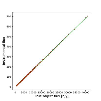
The negative y-intercept is not readily explainable. Intuitively the amount of instrumental flux should be directly proportional to the total astronomical photon count in a given pixel — 0 nJy corresponds to 0 photons from non-background sources, on average, which we would expect to result in 0 instrumental flux units once background subtraction has been performed, as has been done in the coadded images. A significant portion of galaxies in our data set have negative instrumental fluxes according to these calibrations, and a fit that constraints the intercept to be 0 does not reproduce the neat Gaussian distribution of values described in Section A.2. The negative y-intercept appears to indicate some overall background oversubtraction in the coadded images. If the amount of background oversubtraction depended strongly on the overall flux of an object, we would expect to see significant deviations from linearity in the photometric calibration plot. Given the rather high quality of the linear fit (as discussed below, after variance rescaling has been performed), we conclude that the background oversubtraction appears to be relatively constant across all footprints in our data set. We do not know the origin of this apparent oversubtraction.
A.2 Variance plane rescaling
If the total instrumental flux is indeed Gaussian-distributed for every galaxy, with a mean given by the true photometric calibration line, and a variance accurately and completely described by the Pipelines-estimated variance plane, then the distribution of the shifted and scaled quantity defined as should follow a Gaussian distribution with zero mean and unit variance. Figure 16 shows what this distribution actually looks like, both for the variance plane as output by the Pipelines, and for the variance plane multiplied by 2.114. The latter factor is the value of for the calibration fit using the original Pipelines-supplied variance, where the sum of is taken over all points in the fit, and the effective number of degrees of freedom (n.d.o.f.) is equal to the number of points in the fit minus 2. The value of becomes equal to 1 if the original variance plane is multiplied by 2.114; similarly, the overall distribution of values adheres very well to a unit Gaussian when the variance plane is multiplied by the same factor. In other words, the distribution of total instrumental fluxes among the footprints behaves exactly as expected from a simple linear model with Gaussian-distributed errors, with the sizes of the errors described by the coadd variance plane, but only after the Pipelines-supplied variance plane is multiplied by 2.114.
This may mean that the Pipelines-supplied variance plane is simply too small by a factor of 2.114 on average. It may also indicate that the covariance between pixels is too significant to be unaccounted for in a fit such as this: recall that we estimated the variance in the total instrumental flux by simply adding the separate variances in each pixel, which only works under the assumption of zero covariance between pixels. In the more general case of non-zero covariance,
| (A1) |
Here denotes the instrumental flux in pixel , and the sums range over all the pixels in a given footprint. If the sum of the pairwise covariances between pixels in a typical footprint is equal to times the sum of the individual pixel variances, then the variance in the sum of the pixel values will be 2.114 times the sum of the separate variances in each pixel, which is what we observe above. Nevertheless, in this study we have not tried to directly estimate the covariance between pixels in a typical footprint. We have opted to simply scale the Pipelines-supplied variance plane by 2.114 in the likelihood model we use for MCMC fitting, in an effort to fit the total instrumental flux as accurately as possible without modeling the covariance. The differences between the results for our simplified and realistic data sets illustrate the ultimate impact of any deviations between our assumed statistical model and “reality” (as simulated in DC2).
Appendix B Approximate selection corrections to the likelihood
This Appendix extends the discussion in Section 4.3. To compute the effect of on the likelihood, we first rewrite it as
| (B1) |
using Bayes’ theorem. The denominator can be expanded into
| (B2) |
in which the integral is taken over all possible image pixel arrays .
Let be the condition that the pixel values in a given image pass the Pipelines detection algorithm. Let be the condition that, among the true objects the footprint pixels overlap, one of those true objects has a flux at least 50 times larger than the total flux of all the others. Let be the condition that the footprint has exactly one peak. Separating into the three conditions , , and , equation B2 becomes
| (B3) | ||||
Condition , whether the footprint pixel values pass the Pipelines detection algorithm, is a completely deterministic outcome of together with the specific Pipelines algorithm. For any of the pixel arrays we consider, passes the algorithm, and therefore is just 1.171717Technically this is only approximately true, because we define to only include pixels in the footprint, whereas the PSF-convolved image used for detection includes pixels in the convolution that lie outside the footprint. However, only the central core of pixels in any footprint actually passed the Pipelines detection algorithm (recall that footprints are expanded around the detected pixels by 2.4 times the PSF size), and the center of any footprint is so far away from the edge that pixels outside the footprint make a completely negligible contribution to the PSF convolution. The conditional detection probability thus simplifies to
| (B4) |
Now we make some simplifying approximations. First we assume that detection condition , the fact that a footprint overlaps just one true galaxy of real significance, is for practical purposes independent of once and have been specified. We expect that the presence of a secondary, dimmer galaxy in the footprint should not significantly increase the probability of detection unless it lies in a narrow range of brightness values extremely close to the main galaxy (presenting more independent opportunities for detection with comparable likelihood), and/or it overlaps the main galaxy extremely closely along the same line of sight to the telescope (amplifying the detection probability of the regions of overlapping light). We do not rigorously establish the true significance of this interaction here, but it greatly simplifies our analysis to assume total -independence (of , conditioned on and ) and it does not seem to introduce obvious pathologies in the results that follow. Under this assumption, the conditional detection probability further simplifies to
| (B5) |
Another simplifying approximation is that the probability of condition , that the footprint should contain only one peak, is nearly 100% for all possible parameter vectors if conditions and are both met. We directly observe that this is very nearly true in our data set — nearly 100% of data examples for galaxies in the dimmer range, comprising the vast majority our data sets, pass condition if they first pass conditions and , and even the brightest galaxies we consider have at least a 90% chance of doing so. Under the approximation for every case, the conditional detection probability finally simplifies to
| (B6) |
for any and for any likely to be produced from a given . Under the same stipulations, equation B2 simplifies to
| (B7) |
where is the set of all pixel value arrays that satisfy condition . Since does not depend on , it comes out of the integral as a constant. It appears in the denominator of equation B1 for , where it cancels with the equivalent term in the numerator, leaving
| (B8) |
as our final expression for the detection-conditioned likelihood.