Safe Control Design through Risk-Tunable Control Barrier Functions

Abstract

We consider the problem of designing controllers to guarantee safety in a class of nonlinear systems under uncertainties in the system dynamics and/or the environment. We define a class of uncertain control barrier functions (CBFs), and formulate the safe control design problem as a chance-constrained optimization problem with uncertain CBF constraints. We leverage the scenario approach for chance-constrained optimization to develop a risk-tunable control design that provably guarantees the satisfaction of CBF safety constraints up to a user-defined probabilistic risk bound, and provides a trade-off between the sample complexity and risk tolerance. We demonstrate the performance of this approach through simulations on a quadcopter navigation problem with obstacle avoidance constraints.

I INTRODUCTION

Safety is a central consideration in the design of autonomous systems that operate in uncertain and unknown environments, spanning numerous applications such as automated driving, robotics, and unmanned aerial vehicles. The problem of designing controllers that provably guarantee hard constraints on the safety of autonomous systems is a long-studied topic, and has seen a recent resurgence in interest due to advances in learning-based approaches as well as emerging applications such as self-driving cars, where autonomous systems are expected to closely interact with humans in safety-critical settings.

Model-based design approaches to guarantee safety often involve imposing Control Barrier Functions (CBF) constraints [ames2016control] on the control design problem. CBF constraints employ a Lyapunov-like argument to guarantee the invariance of a desired ‘safe set’ under the designed control law, essentially guaranteeing that a system that starts in a safe set always remains in the safe set. We refer the reader to [ames2019control] for a comprehensive survey on the various classes of CBF conditions commonly employed in control design. In situations where the control design problem involves uncertainty in the system dynamics or environment, robust control invariance conditions of a similar nature may be enforced to guarantee safety of the control design [choi2021robust, buch2021robust, sadraddini2017provably, gurriet2018towards, cheng2020safe, cosner2021measurement, santillo2021collision].

While CBF-based designs, including their robust versions, are effective in guaranteeing safety, a key challenge is that they are often conservative, imposing robustness to worst-case uncertainties, which may themselves be difficult to characterize in dynamic environments. Further, they may come at a great efficiency cost (both in terms of time-efficiency and control cost) that can make autonomous task execution practically unviable in several applications. Finally, notions of safety and risk can vary widely by domain. For example, in some applications, small safety constraint violations may be tolerable in order to increase task efficiency. Therefore, it is desirable to introduce probabilistic notions of safety with risk-efficiency tradeoffs that can be selected by designers based on application-specific considerations. In this context, this paper addresses the problem of introducing the notion of tunable risk into the safe control design problem.

Specifically, we consider a class of nonlinear control-affine systems with an additive uncertainty that may arise due to unknown dynamics and/or environmental variables (including obstacles). For this class of systems, we formulate a safe control design problem with uncertain CBF constraints that must be satisfied with a user-defined probabilistic risk bound. We pose this problem in a chance-constrained optimization setting, and propose a sampling-based control design based on the scenario approach [campi2009scenario, calafiore2006scenario, campi2018introduction] that allows the designer to tune the risk bound for safety constraint satisfaction, and provides a trade-off between the risk bound and the sample complexity of the problem. We demonstrate the performance of this design approach by simulation on a quadcopter navigation problem with obstacle avoidance constraints.

I-A Related Work and Contributions

A common approach to safe control design for systems with uncertainties involves modeling the uncertainty by a known process, with Gaussian Process (GP) models receiving significant attention in typical MPC based control designs [hewing2019cautious, bradford2018stochastic], as well as CBF-based designs for safety-critical systems [cheng2019end, cheng2020safe, hu2023safe, luo2022sample]. However, these works do not typically consider the probabilistic notions of safety required to incorporate risk tunability that is the subject of this work. Control designs incorporating probabilistic notions of safety through chance-constrained CBFs have recently been proposed [wang2021chance, blackmore2006probabilistic, nakka2020chance, salehi2022learning, khojasteh2020probabilistic, luo2022sample]. In general, such chance-constrained optimization problems are non-convex, even when the original CBF constraints are convex, and are often NP-hard [ben1998robust, ben2002tractable]. Solutions to such probabalistic safe control design problems typically involve either approximating the uncertainty by GP (or similar) models [salehi2022learning, nakka2020chance, khojasteh2020probabilistic], or deriving convex relaxations or over-approximations that make the problem tractable [wang2021chance, blackmore2006probabilistic]. However, GP models may not hold in several safety-critical applications, and convex over-approximations may lead to conservative designs. In this paper, we introduce a sampling-based safe control design framework based on the scenario-approach for chance-constrained optimization [calafiore2006scenario] that does not make any assumptions regarding the underlying distribution of the uncertainty. The scenario approach has recently been utilized for safety verification with CBFs [akella2022barrier]; however, this work does not address control design, which is the central problem considered in this paper.

In this landscape, the key contribution of this paper is to introduce a framework to design controllers that can guarantee probabilistic notions of safety with user-defined risk bounds, with the advantage that the risk-efficiency and sample complexity trade-offs can be tuned by designers based on domain-specific requirements. We also note that most of the above safe control designs employ projection-based approaches, where a baseline controller (that is designed based on a separate optimization problem or is assumed to be given) is minimally modified through CBF constraints to enforce safety. Such projection-based approaches may result in sub-optimal controllers with reduced performance. In contrast, our approach directly solves a chance-constrained problem to optimize performance metrics while simultaneously guaranteeing safety, without the need for a two-stage solution.

I-B Organization

This paper is organized as follows. Section II formulates the safe control design problem under uncertainties as a chance-constrained optimization problem with control barrier function constraints. Section III provides a risk-tunable design based on the scenario approach to solve the safe control design problem. Section IV demonstrates the design through simulation on a quadcopter navigation problem with uncertain obstacles. The proofs of all the results in this paper are presented in the Appendix.

I-C Notation

We denote the sets of real numbers, positive real numbers including zero, and $n$-dimensional real vectors by $\mathbb{R}$, $\mathbb{R}_{+}$ and $\mathbb{R}^{n}$ respectively. Given a matrix $A\in\mathbb{R}^{m\times n}$, $A^{T}\in\mathbb{R}^{n\times m}$ represents its transpose. A symmetric positive definite matrix $P\in\mathbb{R}^{n\times n}$ is represented as $P>0$ (and as $P\geq 0$, if it is positive semi-definite). The standard identity matrix is denoted by $I$, with dimensions clear from the context. An $(n\times m)$ matrix with all elements equal to 1 is denoted by $\mathbf{1}_{n\times m}$. Similarly, an $(n\times m)$ matrix with all elements equal to zero is denoted by $\mathbf{0}_{n\times m}.$ For any $N_{1},N_{2}\in\mathbb{R}_{+},\begin{pmatrix}N_{1}\\ N_{2}\end{pmatrix}$ represents the number of ways to choose $N_{2}$ items from a set of $N_{1}$ items.

II PROBLEM FORMULATION

We begin by formulating the safe control design problem addressed in this paper.

II-A Dynamics

We consider a nonlinear dynamical system with control-affine dynamics given by,

$$x_{t+1}=f(x_{t})+g(x_{t})u_{t}+d_{t},$$ (1)

where $x_{t}\in X\subset\mathbb{R}^{n}$ is the state, $u_{t}\in U\subset\mathbb{R}^{m}$ is the control input, and $d_{t}\in U\subset\mathbb{R}^{n}$ is an additive disturbance at time $t\in\mathbb{R}_{+}$, and $f:\mathbb{R}^{n}\to\mathbb{R}^{n}$ and $g:\mathbb{R}^{n}\to\mathbb{R}^{n}\times\mathbb{R}^{m}$ are locally Lipschitz continuous. Moreover, we suppose that $U=[u^{l},u^{h}]$, where $u^{l}$ and $u^{h}$ are actuator constraint lower and upper bounds respectively.

Assumption II.1

The dynamical system is assumed to be forward complete, that is, the solution to (1) is defined for all initial conditions $x_{0}\in X$ and all admissible control inputs $u_{t}\in U$ for all time $t\in\mathbb{R}_{+}$.

In this paper, we are interested in designing the control input $u_{t}$ to guarantee the safety of such a system. We begin by defining control barrier functions (CBFs) and associated conditions that we will utilize in formulating the safe control design problem.

II-B Control Barrier Functions (CBF)

Let $\mathcal{S}$ be a safe set, defined by the super-level set of a continuously differentiable function $\bar{h}\colon X\rightarrow\mathbb{R}$ as,

$$\mathcal{S}=\{x\in X\colon\bar{h}(x)\geq 0\}.$$ (2)

If the states always remain within this set, that is, the set is forward invariant, then we can guarantee the safety of the system as follows.

Definition II.2

The dynamical system (1) is said to be safe with respect to set $\mathcal{S}$ if $\mathcal{S}$ is forward-invariant, that is, $\forall x_{0}\in\mathcal{S}$, $x_{t}\in\mathcal{S},\forall t\in\mathbb{R}_{+}$.

A standard approach to establish forward invariance of the safe set $\mathcal{S}$ is to derive sufficient conditions using a Lyapunov-like argument as follows.

Theorem II.3 (Adapted from [agrawal2017discrete])

A continuously differentiable function $\bar{h}\colon X\rightarrow\mathbb{R}$ is a control barrier function for dynamical system (1) and renders the set $\mathcal{S}$ safe if there exists a control input $u_{t}$ and a constant $\eta\in[0,1]$ such that for all $x_{t}\in\mathcal{S}$, we have

$$\bar{h}(x_{t+1})-(1-\eta)\bar{h}(x_{t})\geq 0.$$ (3)

In Theorem II.3, the constant $\eta$ determines how strongly the CBF pushes the states into the safe set [cheng2019end].

II-C Uncertain Control Barrier Functions

With the safe set defined in (2) and the CBF condition defined in Theorem II.3, we now focus on the scenario where there is uncertainty in the CBF condition (3), either due to partially known/uncertain dynamics or due to uncertainties in the operating environment. We define a robust CBF condition as follows.

Theorem II.4

The dynamical system (1) can be rendered safe with safe set $\mathcal{S}$ if, for all uncertainties $d_{t}\in D$, there exists control input $u_{t}\in U$ and a constant $\eta\in(0,1]$ such that

$$L(x_{t},u_{t},d_{t}):=-h(x_{t},u_{t},d_{t})-\eta\bar{h}(x_{t})\leq 0,$$ (4)

where $h(x_{t},u_{t},d_{t}):=\bar{h}(x_{t+1}))-\bar{h}(x_{t})$.

Remark II.5

The CBF condition in Theorem II.3 can be appropriately defined to capture commonly encountered uncertainties in system dynamics and operation as follows:

• Example E1 - Uncertainty in System Dynamics or Environment: Consider the case where part of the system dynamics is unknown, that is, $d_{t}\in D$ is the unknown part of the dynamics in (1). A candidate CBF for such a case is an affine CBF

  $$\bar{h}(x):=p^{T}x+q,$$ (5)

  where $p\in\mathbb{R}^{n}$ and $q\in\mathbb{R}$. Then, the CBF condition in (4) for this case can be written as:

  $$L(x_{t},u_{t},d_{t})= -[p^{T}(f(x_{t})+g(x_{t})u_{t}+d_{t})+q]$$

  $$+(1-\eta)(p^{T}x_{t}+q)\leq 0.$$ (6)

  An identical CBF condition will hold when $d_{t}$ represents an additive exogenous disturbance or uncertainty arising from the interaction of the system with the environment.

• Example E2 - Obstacle Avoidance: We consider the example of a navigation problem with obstacle avoidance constraints, where the safe set is characterized by maintaining a safe distance between an agent (such as a mobile robot or aerial vehicle) and a potentially moving obstacle with position $x^{obs}_{t}\in\mathbb{R}^{n}$ at time $t$. Let the obstacle position be stationary and uncertain, i.e. $x^{obs}_{t}=x^{o}_{t}+d_{t}$ and $x^{obs}_{t+1}=x^{obs}_{t}$, where $x^{o}_{t}$ is known and $d_{t}$ is unknown. For this case, we may define $\bar{h}(x_{t}):=\|x_{t}-x^{obs}_{t}\|^{2}_{2}-r_{s}$, where $r_{s}$ is a user-defined safety margin. Then, the CBF condition in (4) can be written as follows:

  $$L(x_{t},u_{t},d_{t})=$$

  $$-[\|f(x_{t})+g(x_{t})u_{t}-x^{o}_{t}-d_{t}\|^{2}_{2}-r_{s}]$$ (7)

  $$+(1-\eta)\|x_{t}-x^{o}_{t}-d_{t}\|^{2}_{2}-r_{s}\leq 0.$$

II-D Control Design Problem

With this uncertain CBF formulation, the goal is to design control inputs $u_{t}$ that render the system (1) safe $\forall d\in D$. To obtain such control inputs at each time step $t$, we formulate a robust control design problem with constraints given by condition (4) in Theorem II.4.

Consider the robust control design problem (${RCP}^{t}$) at time step $t$ which can be expressed as

$$RCP^{t}:\begin{aligned} \underset{u_{t}}{\mathrm{min}}\ &C(u_{t})\\ s.t.\ \ &L(x_{t},u_{t},d_{t})\leq 0,\ \forall d_{t}\in D,\\ &u^{l}\leq u_{t}\leq u^{h},\end{aligned}$$ (8)

where $C(u_{t})$ is the cost function.

There are several difficulties involved in solving the problem $RCP^{t}$. First, $RCP^{t}$ involves a possibly infinite number of constraints. Even if the problem is assumed to be convex, this class of problems is, in general, NP-hard [ben1998robust, ben2002tractable, el1998robust]. One common approach is to consider the a ‘worst-case’ solution to the RCP, where the CBF constraint in (8) is replaced by $L(x_{t},u_{t},d_{t}^{*})\leq 0$, where $d_{t}^{*}=\max\{d:d\in D\}$. However, such a design would be overly conservative in many applications, and result in decreased performance metrics such as time-efficiency or control effort. Further, in many applications, a small tolerance towards risk is generally acceptable during operation under uncertainty.

We quantify the risk-tolerance in the safe control design problem in terms of violation probability of the CBF condition as follows.

Definition II.6

(Violation Probability) The probability of violation under control input $u_{t}$ is defined as

$$V(u_{t}):=Prob\{d_{t}\in D:L(x_{t},u_{t},d_{t})>0\}.$$ (9)

For a given control input $u_{t}$, the probability that this input violates the CBF constraint $L(x_{t},u_{t},d_{t})\leq 0$ is given by $V(u_{t})$. Assuming a uniform probability density, the violation probability can be interpreted as a measure of the volume of ‘unsafe’ uncertainty parameters $d_{t}$ such that the CBF constraint is violated.

Now, select a tunable user-defined risk bound $\epsilon\in(0,1)$ that quantifies the acceptable violation probability. Note that $\epsilon$ can be selected by the designer based on the application. Then, we define an $\epsilon$-level solution as follows:

Definition II.7

($\epsilon$-level solution) We say that $u_{t}\in U$ is an $\epsilon$-level solution, if $V(u_{t})\leq\epsilon$, $\epsilon\in(0,1)$.

With these definitions, we now reformulate the RCP into a chance constrained problem ($CCP^{t}(\epsilon)$) as follows:

$$CCP^{t}(\epsilon):\underset{u_{t}}{\mathrm{min}} C(u_{t})$$ (10)

$$s.t. Prob\{d_{t}\in D:L(x_{t},u_{t},d_{t})\leq 0\}>1-\epsilon,$$

$$u^{l}\leq u_{t}\leq u^{h}$$

Definition II.8

($\epsilon$-safety) The dynamical system (1) is said to be $\epsilon$-safe if for all $d_{t}\in D$, there exists a control input $u_{t}\in U$ solving the problem $CCP^{t}_{\epsilon}$.

We call the problem of designing a control input $u_{t}$ that solves this probabilistic (chance-constrained) problem as the “risk-tunable ”control design problem, and formally state it as follows.

Risk-Tunable Control Design Problem $\mathcal{P}_{r}:$ Given a user-defined risk tolerance bound $\epsilon$, find control input $u_{t}$ solving $CCP^{t}(\epsilon)$ such that the dynamical system (1) is rendered $\epsilon$-safe at every time $t$.

III RISK-TUNABLE CONTROL DESIGN

In this section, we develop an approach to solve the risk-tunable control design problem $\mathcal{P}_{r}$. We begin by making the following assumptions regarding the convexity of the chance-constrained problem $CCP^{t}_{\epsilon}$.

Assumption III.1

The following is assumed to hold for the problem $CCP^{t}_{\epsilon}$:

• We suppose that the objective function $C(u_{t})$ is a convex function in the control input $u_{t}$.

• Let $u_{t}\subset U$ be a convex and closed set, and let $D\subset\mathbb{R}^{n}$. We assume that $L(x_{t},u_{t},d_{t}):U\times D\rightarrow(-\infty,\infty]$ is continuous and convex in $U$, for any fixed value of $d_{t}\in D$.

Remark III.2

Note that an exact numerical solution of $CCP^{t}(\epsilon)$ is intractable, see [prekopa2013stochastic, vajda2014probabilistic]. Moreover, $CCP^{t}(\epsilon)$ is in general non-convex, even when Assumption III.1 holds.

There are several ways to solve such chance-constrained problems, such as approximating the uncertainty by a known process such as a Gaussian process [hewing2019cautious, bradford2018stochastic], developing convex relaxations or approximations [nemirovski2007convex, blackmore2006probabilistic], and sampling-based approaches [calafiore2006scenario, campi2009scenario]. In this work, we develop a sampling-based design based on the scenario approach [calafiore2006scenario] as follows. The key idea is that if a sufficient number of samples of the uncertainty $d_{t}\in D$ can be extracted, then we can obtain a control which renders the system safe for most uncertainties up to a risk tolerance threshold.

Definition III.3

(Scenario Design) Assume that $N$ independent identically distributed samples $d^{1}_{t},...,d^{N}_{t}$ are drawn according to probability $Prob$. A scenario design problem is given by the convex program:

$$RCP^{t}_{N}\begin{aligned} \underset{u_{t}}{\mathrm{min}}\,&C(u_{t})\\ s.t.\ \ \ &L(x_{t},u_{t},d^{i}_{t})\leq 0,\ \forall i\in\{1,...,N\},\\ &u^{l}\leq u_{t}\leq u^{h}\end{aligned}$$ (11)

Note that the convexity of the problem assumed in Assumption III.1 serves the purpose of enabling the relaxation of $CCP^{t}_{\epsilon}$ to a finite number of constraints and allows for a generalization of the solution to the $CCP^{t}_{\epsilon}$ based on the solution of the simpler $RCP_{N}^{t}$.

Proposition III.4

For the affine CBF defined in (5), (see Example E1 in Remark II.5), $RCP_{N}^{t}$ is convex.

Remark III.5

While we present our results for CBF constraints of the form (4) for simplicity of exposition, the following results are generally applicable to other forms of CBF constraints such as exponential CBFs [ames2019control], provided that they can be designed to satisfy Assumption III.1. Note that Assumption III.1 does not hold for Example E2 in Remark II.5 (the constraints, in that case, can in fact be shown to be concave; see Appendix). However, it is possible to pose obstacle avoidance problems in a convex setting in certain cases using an exponential CBF formulation (one such case is presented in our case study in Section IV to illustrate the broader applicability of the results in this section.)

We now have the following result.

Theorem III.6

For any risk bound $\epsilon\in(0,1)$ and confidence parameter $\beta\in(0,1)$, if

$$N\geq\frac{2}{\epsilon}\ln{\frac{1}{\beta}}+2m+\frac{2m}{\epsilon}\ln{\frac{1}{\beta}},$$ (12)

then, we have that the $RCP_{N}^{t}$ is either infeasible, or if feasible, then

$$Prob^{N}\{V(u_{t}^{*})<\epsilon\}\geq(1-\beta),$$ (13)

that is, its solution $u_{t}^{*}$ renders the system (1) $\epsilon$-safe as in Definition II.8 with probability greater than or equal to $1-\beta$.

Theorem III.6 provides a bound on the number of samples of the uncertainty that are required to guarantee that the control input designed by solving $RCP_{N}^{t}$ can render the system $\epsilon$-safe. In Theorem III.6, the confidence parameter $\beta$ bounds the probability that $u_{t}^{*}$ does not render the system (1) $\epsilon$-safe. In other words, $\beta$ is the probability $Prob^{N}(=Prob\times...\times Prob)$, (N times), of extracting samples of the uncertainty $\{d^{1}_{t},...,d^{N}_{t}\}$ for which the control input $u_{t}^{*}$ does not render the system (1) safe.

We now address the question of when the scenario design problem $RCP_{N}^{t}$ for safe control is guaranteed to have a solution. We show that, under an additional assumption, $RCP_{N}^{t}$ for risk-tunable control design can be shown to always be feasible.

Assumption III.7

For all $d_{t}\in D$, there exists $u_{t}\in U$ such that $\bar{h}\in[m,M]$, $m,M\in\mathbb{R}$, $\forall x\in X$, with $M>m\geq 0$.

With this assumption, we have the following result regarding the solution of $RCP_{N}^{t}$, and therefore, the safe control design problem $CCP^{t}(\epsilon)$.

Theorem III.8

Let Assumptions III.1 and III.7 hold. Then, for any risk bound $\epsilon\in(0,1)$ and confidence parameter $\beta\in(0,1)$, if

$$N\geq\frac{2}{\epsilon}\ln{\frac{1}{\beta}}+2m+\frac{2m}{\epsilon}\ln{\frac{1}{\beta}},$$ (14)

the scenario problem $RCP^{t}_{N}$ is always solvable for any $N$ samples of the uncertainty $\{d^{1}_{t},\ldots,d^{N}_{t}\}$, the solution $u_{t}^{*}$ is unique, and renders the system (1) $\epsilon$-safe in the sense of Definition II.8.

Theorems III.6 and III.8 provide a trade-off between the sample complexity and the achievable risk bound in the safe control design problem, representing an additional handle that can be tuned by designers based on application-specific considerations. Generally, achieving a tighter risk bound will require more samples of the uncertainty.

IV CASE STUDY

$$\mathcal{R}_{wb}:=\begin{bmatrix}\cos{\psi}\cos\theta-\sin{\phi}\sin{\psi}\sin{\theta}&-\cos{\phi}\sin{\psi}&\cos{\psi}\sin{\theta}+\cos{\theta}\sin{\phi}\sin{\psi}\\ \cos{\theta}\sin{\psi}+\cos{\psi}\sin{\phi}\sin{\theta}&\cos{\phi}\cos{\psi}&\sin{\psi}\sin{\theta}-\cos{\psi}\cos{\theta}\sin{\phi}\\ -\cos{\phi}\sin{\theta}&\sin{\phi}&\cos{\phi}\cos{\theta}\end{bmatrix}$$ (15)

We consider a quadcopter navigation problem with an obstacle whose position is uncertain to illustrate our risk-tunable design approach. As described in Remark III.5, the CBF constraints for such obstacle avoidance problems are in general non-convex. However, in some cases, it is possible to develop convex safety conditions. We illustrate such a case in this section, where the nature of the continuous-time dynamics arising from the system physics can be exploited to construct convex CBF conditions for the obstacle avoidance problem that are affine in the control input.

We begin with a dynamical model of the quadcopter derived in [xu2018safe] and summarized here. Let the 3-dimensional position coordinates of the quadcopter along the x-,y-, and z-axis with respect to its body frame $\mathcal{F}_{b}$ of and the world frame of reference $\mathcal{F}_{w}$ be given by $x_{b}:=(x_{b},y_{b},z_{b})$ and $r:=(r_{x},r_{y},r_{z})$ respectively. The rotation matrix for coordinate transformation from the the body frame $\mathcal{F}_{b}$ to the world frame $\mathcal{F}_{w}$ is defined by (15), where $\phi$, $\theta$, and $\psi$ denote the Z-X-Y Euler angles corresponding to the roll, pitch, and yaw of the quadcopter, as depicted in Fig. 1. Therefore, $r=\mathcal{R}_{wb}x_{b}$. Then, the quadrotor dynamics is given by

$$\dot{x} =Ax+Bu$$

$$x =\begin{bmatrix}\dot{r}\\ \ddot{r}\end{bmatrix},A=\begin{bmatrix}\mathbf{0}_{3\times 3}&I\\ \mathbf{0}_{3\times 3}&\mathbf{0}_{3\times 3}\end{bmatrix},B=\begin{bmatrix}\mathbf{0}_{3\times 3}\\ \mathbf{1}_{3\times 3}\end{bmatrix},$$ (16)

where the control input $u$ comprises of the desired acceleration of the quadcopter. The dynamics of the controller under small angle assumptions on the Euler angles (that is, $\sin\hat{e}\approx\hat{e},\cos\hat{e}\approx 1,\hat{e}\in\{\phi,\theta,\psi\}$) evolves according to the following dynamics [mellinger2012trajectory]:

$$u=\begin{bmatrix}\ddot{r}_{1}^{des}\\ \ddot{r}_{2}^{des}\\ \ddot{r}_{3}^{des}\end{bmatrix}=\begin{bmatrix}g(\theta^{des}\cos{\psi^{des}}+\phi^{des}\sin{\psi^{des}}),\\ g(\theta^{des}\sin{\psi^{des}}-\phi^{des}\cos{\psi^{des}})\\ \frac{\sum^{4}_{i=1}F_{i}^{des}}{m}-g\end{bmatrix},$$ (17)

where $m$ is the mass of the quadcopter, $g$ is the acceleration due to gravity, and $\ddot{r}_{i}^{des},i\in\{x,y,z\}$ is the desired acceleration component of the quadcopter in the x-,y-, and z-direction respectively, computed using the desired specifications on the Euler angles $\phi^{des},\theta^{des}$, and $\psi^{des}$, and the desired thrust of each of the four rotors of the quadcopter $F_{i}^{des},i\in\{1,2,3,4\}$.

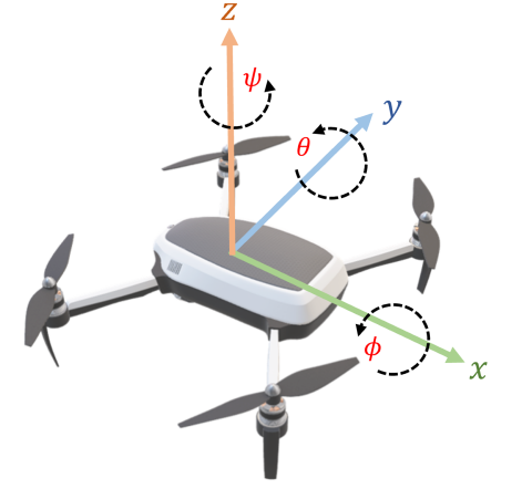
Figure 1: Quadcopter frame and Euler angles.

The objective of the control design is to enable the quadcopter to reach a target position $r_{goal}$, while avoiding an obstacle with position $r_{obs}=\begin{bmatrix}r_{obs_{x}}+d\quad r_{obs_{y}}+d\quad r_{obs_{z}}+d\end{bmatrix}^{T}$, where $d\in D\subset\mathbb{R}$ is the uncertainty in the obstacle position.

For this setting, we choose a safe set

$$\mathcal{S}=\{r:\bar{h}(r)\geq 0\},$$ (18)

where

$$\bar{h}(r)=\left(\frac{r_{ex}}{a}\right)^{4}+\left(\frac{r_{ey}}{b}\right)^{4}+\left(\frac{r_{ez}}{c}\right)^{4}-r_{s},$$ (19)

is the CBF for system (IV), where $r_{ex}=r_{x}-r_{obs_{x}}-d,r_{ey}=r_{y}-r_{obs_{y}}-d,r_{ez}=r_{z}-r_{obs_{z}}-d$, with $a,b,c\in\mathbb{R}_{+}$ can be chosen to represent the shape parameters of a super-ellipsoidal obstacle, and $r_{s}$ is the safe distance from the obstacle to be maintained by the controller.

Now, from (IV) and (19), notice that $\dot{\bar{h}}$ will not depend on the control input $u$, implying that the CBF constraint will be independent of the design variable (the control input). A standard approach to develop a CBF-based safety condition for such a system involves constructing an Exponential Control Barrier Function (ECBF) condition [ames2016control] of the form

$$\ddot{\bar{h}}+K\cdot[\bar{h}\quad\dot{\bar{h}}]^{T}\geq 0,$$ (20)

where $K=[K_{1}\quad K_{2}],K_{1},K_{2}\in\mathbb{R}$, is a design parameter that can be chosen based on the application. Now, we can rewrite (20) as a convex constraint in $u$ as follows.

Proposition IV.1

Define $$L(x,u,d)=-Pu-Q,$$ (21) where $\displaystyle P$ $\displaystyle=\begin{bmatrix}\frac{4r_{ex}^{3}}{a^{4}}&\frac{4r_{ey}^{3}}{b^{4}}&\frac{4r_{ez}^{3}}{c^{4}}\end{bmatrix}$ $\displaystyle Q$ $\displaystyle=\dot{r}^{T}\begin{bmatrix}\frac{12r_{ex}^{2}}{a^{4}}&0&0\\ 0&\frac{12r_{ey}^{2}}{b^{4}}&0\\ 0&0&\frac{12r_{ez}^{2}}{c^{4}}\end{bmatrix}\dot{r}+K_{2}P\dot{r}-K_{1}\bar{h}(r).$ (22) Then, with $L(x,u,d)$ defined in (21), constraint (20) can be rewritten as the affine inequality $L(x,u,d)\leq 0$, where $L(x,u,d)$ is convex in the control input $u$.

The formulation in Proposition IV.1 can be easily implemented numerically in discrete-time as follows. In our simulation, we solve the following optimization problem at every time step $t$:

$$\vspace{0.3cm}(RCP^{t}_{N})_{q}:\quad\begin{aligned} \underset{u_{t}}{\mathrm{min}}\,&(r-r_{goal})^{T}F(r-r_{goal})+u^{T}Gu\\ s.t.\ \ \ &L(x_{t},u_{t},d^{i}_{t})\leq 0,\ \forall i\in\{1,...,N\},\\ &u^{l}\leq u_{t}\leq u^{h},\end{aligned}\vspace{0.1cm}$$ (23)

where $F,G\in\mathbb{R}^{3}$ are positive semi-definite weighting matrices. Note that $(RCP^{t}_{N})_{q}$ satisfies Assumption III.7. Therefore, we extract samples $\{d_{i}^{t}\}$ of the uncertain obstacle position at time $t$ according to Theorem III.8.

The quadcopter dynamical parameters are set up based on [hoshih2020provablyinwild]. For our case study, the additional parameters pertaining to ${(RCP^{t}_{N})}_{q}$ are summarized in Table I. Note that we only control the quadcopter along the x- and y-directions, that is, the number of decision variables is $m=2$ in Theorem III.8.

TABLE I: Simulation Parameters

Parameters	Values
$m$	2
$d_{t}$	$[-0.1,0.1]$
${r_{goal}}_{x}$	7.9
${r_{goal}}_{y}$	8.1
${r_{obs}}_{x}$	7.5
${r_{obs}}_{y}$	7.5
Sampling time	0.1 sec
$r_{s}$	0.4
$K_{1}$	6
$K_{2}$	8
$\beta$	0.01
$a$	0.4
$b$	0.4

With these parameters, the impact of the tunable risk tolerance bound $\epsilon$ on the performance of the control design is shown in Fig. 2. As the risk tolerance is increased, the quadcopter takes a more direct path towards the goal, with some instances where it crosses into the safety margin $r_{s}$ around the obstacle. With a lower risk tolerance ($\epsilon=0.001$ in Fig. 2), the quadcopter takes a much longer duration to reach the goal, following a more circuitous path around the obstacle. Thus, Fig. 2 illustrates how the risk in the design can be traded off for the time performance of the system. Fig. 2 also illustrates the probabilistic nature of the safety guarantees and the role of the uncertainty in the obstacle position in this design, with the same risk bound $\epsilon=0.01$ resulting in two different trajectories with varying levels of safety violations.

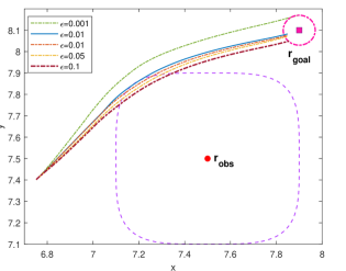
Figure 2: Impact of risk tolerance bound on controller safety and performance.

We now examine how the sample complexity of our design based on Theorem III.6 varies with the risk tolerance bound. Table II lists the number of samples of the uncertainty chosen for each of the risk tolerance bounds $\epsilon$ illustrated in Fig. 2.

TABLE II: Sample Complexity vs Risk Tolerance with $\beta=0.01$

Risk bound $\epsilon$	Number of samples $N$
0.1	216
0.05	484
0.01	3045
0.001	39618

It is observed that the sample complexity increases exponentially as the the risk tolerance bound is decreased. For this case study, we find that the risk tolerance bound $\epsilon=0.05$ provides represents an ideal design choice, bounding the risk of safety violations to under 5%, while maintaining a reasonable trajectory to reach the goal.

V Conclusion

In this work, we develop a safe control design approach where the probability of violation of a CBF-based safety constraint is bounded by a tunable user-defined risk. We developed a design framework based on the scenario approach to solve this problem, and demonstrated the design through simulations on a quadcopter navigation problem with obstacle avoidance constraints. Future directions include extensions to non-convex safety constraints and learning-based control designs.

VI Appendix

1. Proofs of Theorems II.3 and II.4: These results arise directly from the standard definitions of CBFs [ames2019control, agrawal2017discrete].

2. Proof of Proposition III.4: For all $\lambda\in[0,1]$, we have

   $$L(x,\lambda u_{1}+(1-\lambda)u_{2},d)=-p^{T}(f(x)+g(x)(\lambda u_{1}$$

   $$+(1-\lambda)u_{2})+d)-q+(1-\eta)(p^{T}x+q)$$

   which is equal to:

   $$\lambda L(x,u_{1},d)+(1-\lambda)L(x,u_{2},d).$$

   This concludes the proof.

3. Proof of non-convexity of (• ‣ II.5) in Example E2 in Remark II.5: For all $\lambda\in[0,1]$,

   $$L(x,\lambda u_{1}+(1-\lambda)u_{2},d)=-\|f(x)+g(x)(\lambda u_{1}+$$

   $$(1-\lambda)u_{2})-x^{o}-d\|^{2}_{2}+r_{s}+(1-\eta)(\|x-x^{o}-d\|^{2}_{2}$$

   $$-r_{s})$$

   Using $\|v_{1}+v_{2}\|\leq\|v_{1}\|+\|v_{2}\|$, $\forall v_{1},v_{2}\in\mathbb{R}^{n}$, we conclude that

   $$L(x,\lambda u_{1}+(1-\lambda)u_{2},d) \geq$$ (24)

   $$\lambda L(x,u_{1},d) +(1-\lambda)L(x,u_{2},d).$$

   Therefore, $L(x,u,d)$ is concave.

4. Proof of Theorem III.6: The proof of this result is along the lines of [calafiore2006scenario] as follows. We omit the dependence of all variables on time $t$ for simplicity of notation. Define

   $$\mathcal{X}_{i}:=\{u\in U\ :L(x,u,d^{i})\leq 0\}.$$ (25)

   From Assumption III.1, $\{\mathcal{X}_{i}\}$, $\forall i\in[1,N+2m]$ are the convex sets $\mathbb{R}^{m}$ defined by the $2m$ actuator constraints, that is, $u\in U=[u^{l},u^{h}]$ and the $N$ CBF constraints in $RCP_{N}^{t}$. Now, we set up the convex optimization problems $\mathcal{P}$ as

   $$\mathcal{P}:\begin{aligned} \underset{u_{t}}{\mathrm{min}}\ &C(u_{t})\\ s.t.\ &u_{t}\in\bigcap_{i=\{1,...,N+2m\}}\mathcal{X}_{i},\end{aligned}$$ (26)

   and $\mathcal{P}_{k}$, $k\in[1,N+2m]$, by removing the $k^{th}$ constraint as

   $$\mathcal{P}_{k}:\begin{aligned} \underset{u_{t}}{\mathrm{min}}\ &C(u_{t})\\ s.t.\ &u_{t}\in\bigcap_{i=\{1,...,N+2m\}\setminus k}\mathcal{X}_{i}\end{aligned}$$ (27)

   Suppose $RCP_{N}^{t}$ is feasible, and $u_{t}^{*}$ is the optimal solution to $\mathcal{P}$, and $u_{k}^{*}$ is the optimal solution to $\mathcal{P}_{k}$. Then, we define the $k^{th}$ constraint as the support constraint if $C(u^{*}_{k})<C(u^{*})$. It can be shown that the number of support constraints for problem $\mathcal{P}$ is at most $m$ [calafiore2006scenario, Theorem 3].

   Given N scenarios $\{d^{1},...,d^{N}\}$, select a subset $\mathcal{I}=\{i_{1},...,i_{m}\}$ of $m$ indices from $1,...,N+2m$ and let $\hat{u}_{I}^{*}$ be the optimal solution of ${RCP_{I}^{t}}$ defined as

   $$RCP_{I}^{t}:\begin{aligned} &\underset{u_{t}}{\mathrm{min}}\ C(u_{t})\\ &s.t.\ L(u,d^{i})\leq 0,\ \forall i\in\{1,...,m\},\\ &u^{l}\leq u\leq u^{h}.\end{aligned}$$ (28)

   Suppose that $\Delta^{N}:=\{d^{i}\}_{i=1,...,N}$ is the set of all possible $N$ samples drawn from the set $D$. Then, based on $\hat{u}_{I}^{*}$ we next introduce a subset $\Delta^{N}_{I}$ of the set $\Delta^{N}$ defined as

   $$\Delta^{N}_{I}=\{d^{1},...,d^{N}:\hat{u}_{I}^{*}=\hat{u}_{N}^{*}\}$$ (29)

   where $\hat{u}_{N}^{{*}}$ is the optimal solution with all the $N$ constraints $\{d^{1},...,d^{N}\}$. Moreover, suppose $\mathcal{I}$ is a collection of all possible choices of $m$ indices from $1,...,N+2m$, then $\mathcal{I}$ contains $\begin{pmatrix}N+m\\ m\end{pmatrix}$ sets and

   $$\Delta^{N}=\bigcup_{I\in\mathcal{I}}\Delta_{I}^{N}.$$ (30)

   Now suppose, $B:=\{d^{1},...,d^{N}:V(\hat{u}_{N}^{*})>\epsilon\}$ and $B_{I}:=\{d^{1},...,d^{N}:V(\hat{u}_{I}^{*})>\epsilon\}$. Then,

   $$B=\bigcup_{I\in\mathcal{I}}(B_{I}\bigcap\Delta^{N}_{I}).$$ (31)

   A bound for $Prob^{N}(B)$ is now obtained by bounding $Prob(B_{I}\bigcap\Delta_{I}^{N})$ and then summing over $I\in\mathcal{I}$.

   Following a similar argument as in the proof in [calafiore2006scenario, Appendix B], we have

   $$Prob^{N}(B)\leq\sum_{I\in\mathcal{I}}Prob^{N}(B_{I}\bigcap\Delta^{N}_{I})$$ (32)

   which can further be bounded using the fact that the collection $\mathcal{I}$ has $\begin{pmatrix}N+m\\ m\end{pmatrix}$ sets as follows:

   $$\sum_{I\in\mathcal{I}}Prob^{N}(B_{I}\bigcap\Delta^{N}_{I})<\begin{pmatrix}N+m\\ m\end{pmatrix}(1-\epsilon)^{N+m}.$$ (33)

   Then, following the algebraic manipulations in [calafiore2006scenario, Appendix B] $N\geq\frac{2}{\epsilon}\ln{\frac{1}{\beta}}+2m+\frac{2m}{\epsilon}\ln{\frac{1}{\beta}}$, we have $\begin{pmatrix}N+m\\ m\end{pmatrix}(1-\epsilon)^{N+m}\leq\beta$. That is to say that

   $$Prob^{N}(B)<\beta.$$ (34)

   Now, if $RCP_{N}^{t}$ is only feasible on a subset $F_{s}\subset\Delta^{N}$, then, the same arguments hold to prove that the bound (34) holds in the set $F_{s}$, with $B:=\{(d^{1},...,d^{N})\in F_{s}:V(\hat{u}_{N}^{*})>\epsilon\}$, which concludes the proof.

5. Proof of Theorem III.8:

   Since $h\in[m,M]$, $\forall u\in[u^{l},u^{h}]$, we note that

   $$-L(x_{t},u_{t},d_{t})\geq m-(1-\eta)M,$$

   $\forall d\in D$ and $\forall t\in\mathbb{R}_{+}$. Then, we can always select $\eta$, such that $1\geq\eta\geq 1-\frac{m}{M}$ to ensure

   $$L(x_{t},u_{t},d_{t})\leq 0,$$

   which implies that $RCP^{t}_{N}$ is feasible for any $N$ samples of uncertainty. Moreover because $h$, and therefore $L$ is bounded $\forall u\in[u^{l},u^{h}],d\in D$, and $RCP^{t}_{N}$ is convex, feasible and bounded, a unique solution exists.

6. Proof of Proposition IV.1: Differentiating (19), we have

   $$\dot{\bar{h}}(r)=P\dot{r},$$ (35)

   where $P$ is defined in (IV.1) (since $\dot{r}_{goal}=0$). Further differentiating (19), we can obtain

   $$\ddot{\bar{h}}(r)=\dot{r}^{T}Qr+Pu.$$ (36)

   Substituting (35) and (36) in (20) and collecting the terms involving the conrol input $u$, we obtain

   $$-Pu\leq\dot{r}^{T}\tilde{Q}r+K_{1}\bar{h}+K_{2}P\dot{r},$$ (37)

   where $\tilde{Q}=\begin{bmatrix}\frac{12r_{ex}^{2}}{a^{4}}&0&0\\ 0&\frac{12r_{ey}^{2}}{b^{4}}&0\\ 0&0&\frac{12r_{ez}^{2}}{c^{4}}\end{bmatrix}$ Defining $L(x,u,d)=-Pu-Q$, where $Q=\dot{r}^{T}\tilde{Q}r+K_{1}\bar{h}+K_{2}P\dot{r}$, noticing that $L(x,u,d)$ is affine in $u$, and invoking Proposition (III.4) completes the proof.