Impact of strain on the SOT-driven dynamics of thin film Mn₃Sn

Abstract

Mn₃Sn, a metallic antiferromagnet with an anti-chiral 120^∘ spin structure, generates intriguing magneto-transport signatures such as a large anomalous Hall effect, spin-polarized current with novel symmetries, anomalous Nernst effect, and magneto-optic Kerr effect. When grown epitaxially as MgO(110)[001]$\parallel$ Mn₃Sn($0\bar{1}\bar{1}0$)[0001], Mn₃Sn experiences a uniaxial tensile strain, which changes the bulk six-fold anisotropy landscape to a perpendicular magnetic anisotropy with two stable states. In this work, we investigate the field-assisted spin orbit-torque (SOT)-driven response of the order parameter in single-domain Mn₃Sn with uniaxial tensile strain. We find that for a non-zero external magnetic field, the order parameter can be switched between the two stable states if the magnitude of the input current is between two field-dependent critical currents. Below the lower critical current, the order parameter exhibits a stationary state in the vicinity of the initial stable state. On the other hand, above the higher critical current, the order parameter shows oscillatory dynamics which could be tuned from the 100’s of megahertz to the gigahertz range. We obtain approximate expressions of the two critical currents and find them to agree very well with the numerical simulations for experimentally relevant magnetic fields. We also obtain unified functional form of the switching time versus the input current for different magnetic fields. Finally, we show that for lower values of Gilbert damping ($\alpha\leq 2\times 10^{-3}$), the critical currents and the final steady states depend significantly on the damping constant. The numerical and analytic results presented in our work can be used by both theorists and experimentalists to understand the SOT-driven order dynamics in PMA Mn₃Sn and design future experiments and devices.

I Introduction

Antiferromagnets (AFMs) are a class of magnetic materials that produce negligible stray fields, are robust to external magnetic field perturbations, and exhibit resonant frequency in the terahertz (THz) regime. These distinctive properties are a consequence of a strong exchange interaction between the uniquely arranged spins of the neighboring atoms, and a negligible net macroscopic magnetization [1, 2, 3, 4]. AFMs are, therefore, considered as promising candidates for building next generation magnonic devices, high-density memory devices, and ultrafast signal generators. [5] Among the various possible AFMs, noncollinear but coplanar metallic AFMs of the form Mn₃X, with a triangular spin structure, have recently been explored extensively, owing to their intriguing magneto-transport characteristics such as a large spin Hall effect (SHE) [6], anomalous Nernst effect (ANE), anomalous Hall effect (AHE) [7, 8, 9, 10], and magneto-optical Kerr effect (MOKE) [11], ferromagnet-like spin-polarized currents [12, 13], and a finite tunneling magnetoresistance (TMR) [14, 15]. These noncollinear AFMs are chiral in nature and could be further classified as positive (X = Ir, Pt, Rh) or negative (X = Sn, Ge, Ga) chirality materials based on the type of spin interaction [16].

Here, we focus on the negative chirality material Mn₃Sn owing to various factors. Mn₃Sn has a high Néel temperature of approximately $420-430~{}\mathrm{K}$ [17, 11]. Recent experiments have demonstrated that the magnetization in Mn₃Sn can be switched between stable states using spin-orbit torque (SOT) in a bilayer setup of heavy metal (HM) and Mn₃Sn [18, 19, 20, 21, 22, 23]. The charge current density required in these switching experiments was found to be approximately $10^{6}-10^{7}~{}\mathrm{A/cm^{2}}$ [19, 20, 21], which is smaller than or comparable to that in the case of most SOT-driven ferromagnets ($\sim 10^{7}-10^{8}~{}\mathrm{A/cm^{2}}$) [24]. SOT-generated oscillatory dynamics of the order parameter in Mn₃Sn have also been investigated experimentally and theoretically [19, 25, 26], where it was shown that the oscillation frequency could be tuned from 100’s of MHz to GHz range for the charge current density of the order of $10^{6}-10^{7}~{}\mathrm{A/cm^{2}}$. Contrary to collinear AFMs, the magnitude of anomalous Hall conductivity in Mn₃Sn has been reported to be quite large, roughly $30-40~{}\mathrm{\Omega^{-1}\cdot cm^{-1}}$ at $300~{}\mathrm{K}$ [27, 22]. Furthermore, application of small in-plane uniaxial strain of $\sim 0.1\%$ was recently shown to control the magnitude and sign of the anomalous Hall signal in Mn₃Sn, owing to its piezomagnetic properties [28]. More recently, thin films of Mn₃Sn, grown epitaxially on MgO(110)[001] substrate, were found to exhibit perpendicular magnetic anisotropy (PMA) due to the in-plane tensile strain arising from the lattice mismatch between Mn₃Sn and MgO [22]. Finally, a TMR of approximately $2\%$ was recently reported at room temperature in an all-antiferromagnetic tunnel junction comprising thin films of Mn₃Sn/MgO/Mn₃Sn [15]. These experimental developments in both the manipulation and detection of magnetization state in thin films of Mn₃Sn make it a prospective candidate for future spintronic devices such as high-density antiferromagnetic memory and ultrafast nano-oscillator.

In this work, we theoretically investigate the magnetic field-assisted SOT-driven dynamics in thin films of monodomain strained-Mn₃Sn with two stable states. Recent experimental works have revealed that deterministic switching between the stable states of Mn₃Sn requires an external symmetry-breaking magnetic field in the direction of the current flow [18, 19, 20, 21, 22, 23]. Furthermore, the threshold current density for magnetization switching was found to be minimum for the spin polarization perpendicular to the Kagome lattice [19, 25, 22]. In the same configuration, but in the absence of a magnetic field, chiral rotation of the order parameter of Mn₃Sn have also been experimentally reported [25]. More recently, experiments by Higo et al. revealed the possibility of tuning the mode of dynamics, that is, either deterministic switching or chiral oscillations, in uniaxially strained-Mn₃Sn exhibiting PMA, by tuning the applied magnetic field or the input current [22]. However, a detailed analysis of the relationship between the mode of dynamics on the external stimuli is lacking. In particular, the dependence of the threshold currents to excite switching or oscillation dynamics on the material parameters and external field has not been presented in previous works. Finally, the dependence of the switching time and the oscillation frequency on material parameters and external stimuli is also lacking.

Here, we address both the numerical and analytical aspects of current-driven dynamics in a predominantly two-fold anisotropic thin film of single-domain Mn₃Sn with non-vanishing net magnetization. The two-fold anisotropy in Mn₃Sn is a consequence of the epitaxial strain resulting from a lattice mismatch between the substrate and the AFM thin film. In addition, we also consider a weak six-fold anisotropy, which arises due to the frustrated structure of bulk Mn₃Sn, in our analysis (Section III). Such a system with dominant two-fold anisotropy and weak six-fold anisotropy has also been considered in Ref. [29]; therein, however, only the pulsed-SOT-driven switching dynamics was considered. Other previous theoretical works on the current-driven switching and oscillation dynamics in both collinear and noncollinear AFMs have only explored two-fold anisotropic systems with zero net magnetization [30, 31, 32]. Another work focused only on the numerical aspects of pulsed-SOT switching in NiO with six-fold anisotropy [33]. Our previous work focusing on both the numerical and analytical aspect of current-driven dynamics in six-fold anisotropic Mn₃Sn presents an accurate model of threshold current, oscillation frequency, and the relation between the magnitude and the duration of an input current pulse required to switch between the six stable states [26].

Unlike prior works, the models developed in our present work elucidate the impact of magnetic field as well as the differences in the dynamics resulting from the magnitude and nature of strain, i.e., tensile versus compressive (Section IV and supplementary material). Impact of damping on the dynamics is also examined in the case of monodomain Mn₃Sn with tensile strain (Section V). Our results establish connections with experimental results reported in the literature. A brief discussion of the AHE and the TMR schemes to detect the state of the order parameter in Mn₃Sn is presented in the supplementary material.

II Properties of Mn₃Sn

Below its Néel temperature, Mn₃Sn crystallizes into a hexagonal Kagome $D0_{19}$ lattice and can only be stabilized in slight excess of Mn atoms. The Mn atoms are located at the corners of the hexagons whereas the Sn atoms are located at their respective centers. Such lattices are stacked along the $c$ axis $([0001]$ direction$)$ in an ABAB arrangement. A simple representation of the crystal structure is presented in Fig. 1.

In the Kagome plane, the magnetic moments on the Mn atoms form a geometrically frustrated noncollinear triangular spin structure, with spins on the nearest neighbors aligned at an angle of approximately $120^{\circ}$ with respect to each other [34]. These spins are slightly canted toward the in-plane easy axes resulting in a small net magnetization, which is six-fold degenerate in the Kagome plane [35]. The chirality of the degenerate spin structure breaks the time-reversal symmetry (TRS) and leads to the momentum-dependent nonzero Berry curvature, which enhances the magneto-transport signals such as AHE and ANE [7, 35]. Switching from one magnetization state to another reverses the sign of the Berry curvature and hence that of the magneto-transport signals that are odd with respect to the Berry curvature. The TMR in Mn₃Sn also originates from the TRS breaking and the momentum-dependent spin splitting of electronic band structure [15, 36].

The application of a small $\quantity(<1\%)$ in-plane compressive or tensile uniaxial strain to the Mn₃Sn crystal engenders its bond lengths unequal, and hence the strength of the in-plane exchange interactions in different directions [28]. As a result, the crystal symmetry changes from the weak six-fold degeneracy to predominantly a stronger two-fold degeneracy, while the magnitude of the net magnetization is increased proportional to the strain [28]. This change in the degeneracy of the order parameter changes the AHE signal (magnitude and sign) as the order parameter is coupled to the Hall conductivity [29].

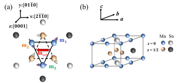
Figure 1: (a) Atomic and one of the six possible spin arrangements in the basal plane of bulk Mn₃Sn. (b) Unit cell of Mn₃Sn.

III Free Energy Model and Ground States

For a single-domain particle of uniaxially strained-Mn₃Sn, composed of three interpenetrating sublattices, the free energy density can be defined as [28, 22, 37]

$$\begin{split}&F\quantity(\mathbf{m}_{1},\mathbf{m}_{2},\mathbf{m}_{3})=J_{E}\left(\quantity(1+\delta_{E})\mathbf{m}_{1}\dotproduct\mathbf{m}_{2}+\mathbf{m}_{2}\dotproduct\mathbf{m}_{3}\right.\\ &\left.+\mathbf{m}_{3}\dotproduct\mathbf{m}_{1}\right)+D_{M}\mathbf{z}\dotproduct\left(\mathbf{m}_{1}\crossproduct\mathbf{m}_{2}+\mathbf{m}_{2}\crossproduct\mathbf{m}_{3}\right.\\ &\left.+\mathbf{m}_{3}\crossproduct\mathbf{m}_{1}\right)-\sum_{i=1}^{3}\quantity(K_{e}\quantity(\mathbf{m}_{i}\dotproduct\mathbf{u}_{e,i})^{2}+M_{s}\mathbf{H}_{a}\dotproduct\mathbf{m}_{i}),\end{split}$$ (1)

where $\mathbf{m}_{1},\mathbf{m}_{2}$, and $\mathbf{m}_{3}$ are the magnetization vectors corresponding to the three sublattices, while $J_{E}(>0)$, $D_{M}(>0)$, and $K_{e}(>0)$ are the symmetric exchange interaction constant, asymmetric Dzyaloshinskii-Moriya interaction (DMI) constant, and single-ion uniaxial magnetocrystalline anisotropy constant, respectively. Each magnetization vector has a constant saturation magnetization, $M_{s}$. Here, it is assumed that the uniaxial strain acts along the x-direction in Fig. 1(a). The effect of this uniaxial strain is then included in the empirical parameter $\delta_{E}$—a positive (negative) value indicates a stronger (weaker) exchange interaction between the sublattices $\mathbf{m}_{1}$ and $\mathbf{m}_{2}$ [28, 22]. Therefore, a positive (negative) $\delta_{E}$ corresponds to a shorter (longer) bond length and hence compressive (tensile) strain between $\mathbf{m}_{1}$ and $\mathbf{m}_{2}$. The last term in Eq. (1) is the Zeeman energy due to the externally applied magnetic field $\mathbf{H}_{a}$. Finally, $\mathbf{u}_{e,i}$ is the local easy axis corresponding to $\mathbf{m}_{i}$. The easy axes are given as $\mathbf{u}_{e,1}=-(1/2)\mathbf{x}+(\sqrt{3}/2)\mathbf{y}$, $\mathbf{u}_{e,2}=-(1/2)\mathbf{x}-(\sqrt{3}/2)\mathbf{y}$ and $\mathbf{u}_{e,3}=\mathbf{x}$. Mn₃Sn is an exchange dominant AFM such that $J_{E}\gg D_{M}\gg K_{e}$. Typical values of the material parameters of Mn₃Sn, considered in this work, are listed in Table 1.

In the case of bulk Mn₃Sn, where $\delta_{E}=0$, the hierarchy of energy interactions $\quantity(J_{E}\gg D_{M}\gg K_{e})$ ensures that the three sublattice vectors in the ground state are confined to the x-y plane at an angle of $\frac{2\pi}{3}$ with respect to each other. In particular, the DMI enforces a clockwise ordering between the vectors $\mathbf{m}_{1}$, $\mathbf{m}_{2}$, and $\mathbf{m}_{3}$, and leads to six-fold energy degeneracy since the local easy axes $\mathbf{u}_{e,1}$, $\mathbf{u}_{e,2}$, and $\mathbf{u}_{e,3}$ follow a counterclockwise ordering [38, 39]. In each of these six minimum energy states, only one of the $\mathbf{m}_{i}$’s is along its respective $\mathbf{u}_{i}$. The introduction of in-plane uniaxial strain, externally or due to epitaxial growth, changes the six-fold degeneracy to two-fold since the exchange interactions become unequal [28, 22, 29]. To verify these claims, differentiate between the two types of strain, and understand the role of the external magnetic field on the static properties of Mn₃Sn, we minimize Eq. (1) with respect to $\mathbf{m}_{i}$.

The ground states of Mn₃Sn for compressive and tensile strains, in the absence of any magnetic field $\quantity(\mathbf{H}_{a}=0)$, are shown in Fig. 2. The three sublattice vectors are in the Kagome plane, which is assumed to coincide with the x-y plane. In the case of compressive strain, only $\mathbf{m}_{3}$ coincides with its easy axis, leading to a two-fold degeneracy, as shown in Fig. 2(a, b). On the other hand, in the case of tensile strain, no sublattice vector coincides with its easy axis. Instead, $\mathbf{m}_{3}$ is perpendicular to its easy axis, as shown in Fig. 2(c, d). In bulk Mn₃Sn a small non-zero in-plane net magnetization, $\mathbf{m}=\frac{\mathbf{m}_{1}+\mathbf{m}_{2}+\mathbf{m}_{3}}{3}$, has been shown to exist [38, 26]. Our simulation reveals that strained-Mn₃Sn also hosts a net magnetization which is parallel (antiparallel) to $\mathbf{m}_{3}$ in the case of the compressive (tensile) strain. We find that for $|\delta_{E}|=10^{-3}$, which represents a uniaxial strain of $0.1\%$, the norm of the net magnetization increases from the bulk value of $\norm{\mathbf{m}}\approx 3.66\times 10^{-3}$ to $\norm{\mathbf{m}}\approx 3.95\times 10^{-3}$ $\quantity(\norm{\mathbf{m}}\approx 3.92\times 10^{-3})$ in the case of compressive (tensile) strain. Finally, we find that the angle between the sublattice vectors is slightly different from $120^{\circ}$. In the case of compressive (tensile) strain, $\eta_{12}\approx 0.78^{\circ}\quantity(-0.78^{\circ})$ and $\eta_{23}=\eta_{31}\approx-0.39^{\circ}\quantity(0.39^{\circ})$, where $\eta_{ij}=\cos^{-1}{(\mathbf{m}_{i}\dotproduct\mathbf{m}_{j})}-\frac{2\pi}{3}$. For both compressive and tensile strain, $\eta_{12}+\eta_{23}+\eta_{31}=0$.

Table 1: List of material parameters for the AFM, Mn₃Sn, and the heavy metal (HM), which is chosen as W, in the SOT device setup.

Parameters	Definition	Values	Ref.
$J_{E}~{}(\mathrm{J/m^{3}})$	Exchange constant	$2.4\times 10^{8}$	[16]
$D~{}(\mathrm{J/m^{3}})$	DMI constant	$2\times 10^{7}$	[16]
$K_{e}~{}(\mathrm{J/m^{3}})$	Uniaxial anisotropy constant	$3\times 10^{6}$	[16]
$M_{s}~{}(\mathrm{A/m})$	Saturation magnetization	$1.3\times 10^{6}$	[16]
$|\delta_{E}|$	Strain parameter	$10^{-3}$	[22]
$\alpha$	Gilbert damping	$0.003$	[18]
$\theta_{\mathrm{SH}}$	Spin Hall angle for HM	$0.06$	[22]

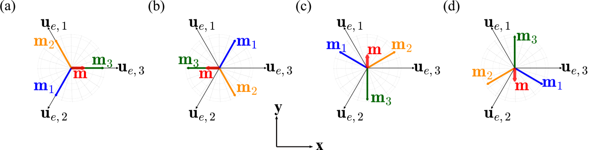
Figure 2: Equilibrium states in single-domain Mn₃Sn crystal under compressive (a, b) and tensile (c, d) strains. The sublattice vectors lie in the Kagome plane which is assumed to coincide with the x-y plane. (a, b) Only $\mathbf{m}_{3}$ coincides with its easy axis. (c, d) None of the sublattice vectors coincide with their local easy axes. Instead, tensile strain forces $\mathbf{m}_{3}$ perpendicular to its easy axis. The two equilibrium states for compressive as well as tensile strains are separated by $180^{\circ}$ with respect to each other. A small in-plane average magnetization $\mathbf{m}$, parallel (antiparallel) to $\mathbf{m}_{3}$ in the case of compressive (tensile) strain, exists in all the cases. The magnitude of $\mathbf{m}$ depends on the strength of the strain. Here, $\mathbf{m}$ is not drawn to scale but magnified by $100\times$ for the purpose of clear representation.

An external magnetic field, when applied to the thin film of Mn₃Sn, changes the energy of the system and therefore the ground states. Here, we only consider external fields in the Kagome plane as $\mathbf{H}_{a}=H_{0}\quantity(\cos{(\varphi_{H})},\sin{(\varphi_{H})},0)$, where $\varphi_{H}$ is the angle between the magnetic field and the x-axis. Figure 3(a) shows the ground states of Mn₃Sn when $\mathbf{H}_{a}=\quantity(0,0.1~{}\mathrm{T},0)$ is applied to the equilibrium state of Fig. 2(a) whereas Fig. 3(b) shows the ground state when $\mathbf{H}_{a}=\quantity(-0.1~{}\mathrm{T},0,0)$ is applied to the equilibrium state of Fig. 2(c). In both the cases $\mathbf{m}$ tilts towards the magnetic field, while the sublattice vectors either tilt towards $\mathbf{H}_{a}$ or away from it, in order to lower the energy of the system. As compared to the equilibrium states of Fig. 2, the angles between the sublattice vectors change when an external field is applied, although by a negligible amount. However, if the applied field is large it could disturb the $120^{\circ}$ relative orientation of the magnetic moments. Therefore, in this work, we consider relatively small magnetic fields that are sufficient to aid the dynamics (discussed later in Sec. IV) without disturbing the antiferromagnetic order, viz. $J_{E}\gg D_{M}\gg H_{0}M_{s}$.

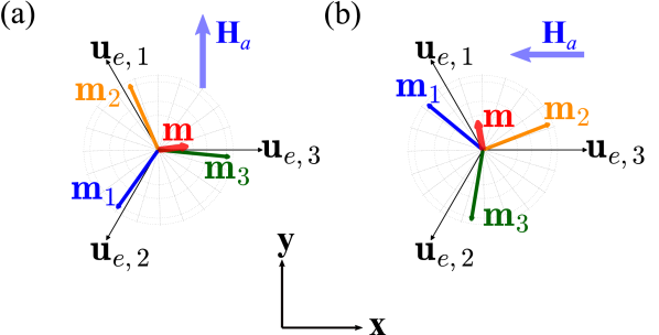
Figure 3: Ground states of monodomain Mn₃Sn crystal, with (a) compressive strain and (b) tensile strain, under the effect of in-plane external magnetic field, $\mathbf{H}_{a}=H_{0}\quantity(\cos{(\varphi_{H})},\sin{(\varphi_{H})},0)$. In both the cases $\mathbf{m}$ tilts towards $\mathbf{H}_{a}$. Here, $\norm{H_{a}}=0.1~{}\mathrm{T}$ while $\mathbf{m}$ is magnified by $100\times$ for the purpose of clear representation in both the cases.

III.1 Perturbative Analysis

For a clear understanding of the aforementioned ground states of the monodomain strained-Mn₃Sn, we consider the perturbative approach presented in Refs. [38, 39, 37]. Firstly, we define the sublattice vector as $\mathbf{m}_{i}=\quantity(\sqrt{1-u_{i}^{2}}\cos{\quantity(\varphi_{i})},\sqrt{1-u_{i}^{2}}\sin{\quantity(\varphi_{i})},u_{i})$, where $\varphi_{i}$ and $u_{i}$ are its azimuthal angle and the z-component, respectively. Secondly, we define the experimentally relevant cluster magnetic octupole moment [40, 37] as $\mathbf{m}_{\mathrm{oct}}=\frac{1}{3}\mathcal{M}_{zx}\quantity[R(\frac{2\pi}{3})\mathbf{m}_{1}+R(-\frac{2\pi}{3})\mathbf{m}_{2}+\mathbf{m}_{3}]$. Here, $\mathbf{m}_{1}$ and $\mathbf{m_{2}}$ are rotated by $+2\pi/3$ and $-2\pi/3$, respectively, while the y-component of the resultant vector undergoes a mirror operation with respect to x-z plane [37]. This ensures that the octupole and the sublattice vectors are coplanar, and $\varphi_{\mathrm{oct}}=-\frac{\varphi_{1}+\varphi_{2}+\varphi_{3}}{3}$, where $\varphi_{\mathrm{oct}}$ is the azimuthal angle of the magnetic octupole. Thirdly, we define $\varphi_{i}=-\varphi_{\mathrm{oct}}-\frac{2\pi i}{3}+\eta_{i}$, where $\eta_{i}$ is a small angle ($\eta_{i}\ll 2\pi/3$) that includes the effect of small deviation from the rigid $120^{\circ}$ configuration due to both the frustrated bulk structure and the strain. Here, $\eta_{i}$ is linearly independent of $\varphi_{\mathrm{oct}}$ and $\eta_{1}+\eta_{2}+\eta_{3}=0$. Finally, we use the perturbative approach, as outlined in the supplementary material, to arrive at an energy landscape, which is a function of $\varphi_{\mathrm{oct}}$ [38, 39, 37] and is given as

$$\begin{split}&F\quantity(\varphi_{\mathrm{oct}})\approx-\frac{3A}{2}\cos{\quantity(2\varphi_{\mathrm{oct}})}-\frac{B}{2}\cos{\quantity(6\varphi_{\mathrm{oct}})}\\ &-3M_{s}H_{0}\quantity(C\cos{\quantity(\varphi_{\mathrm{oct}}-\varphi_{H})}+D\cos{\quantity(\varphi_{\mathrm{oct}}+\varphi_{H})}),\end{split}$$ (2)

where $A=\frac{2J_{E}\delta_{E}K_{e}}{3\quantity(J_{E}+\sqrt{3}D_{M})}$, $B=\frac{\quantity(3J_{E}+7\sqrt{3}D)K_{e}^{3}}{9\quantity(J_{E}+\sqrt{3}D_{M})^{3}}$, $C=\frac{K_{e}}{3\quantity(J_{E}+\sqrt{3}D_{M})}$, and $D=\frac{J_{E}\delta_{E}}{3\quantity(J_{E}+\sqrt{3}D_{M})}$. The constant terms are not shown here as they do not affect the final orientation of the magnetic octupole in the Kagome plane.

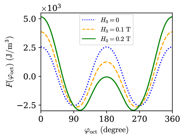
Figure 4: Energy density as a function of the octupole angle of a monodomain Mn₃Sn with tensile strain for different applied magnetic field, $H_{0}$, along the -x-direction ($\varphi_{H}=180^{\circ}$). External magnetic field breaks the symmetry of the system, and therefore barrier height reduces at $\varphi_{\mathrm{oct}}=\pi$ but increases at $\varphi_{\mathrm{oct}}=0$, as $H_{0}$ increases.

For $H_{0}=0$ in Eq. (2) and $|A|\gg B$, the $\cos{\quantity(2\varphi_{\mathrm{oct}})}$ term dominates over the $\cos{\quantity(6\varphi_{\mathrm{oct}})}$ term. As a result, compressive (tensile) strain leads to two minimum energy equilibrium states of the magnetic octupole corresponding to $\varphi_{\mathrm{oct}}=0$ $(\pi/2)$ and $\varphi_{\mathrm{oct}}=\pi$ $(3\pi/2)$, as shown in Fig. 2. On the other hand, when a small magnetic field is turned on ($H_{0}>0$), the energy of the system changes, and two ground states of the octupole moment corresponding to the minimum of Eq. (2) are obtained. Firstly, these ground states are different from the equilibrium states, if $\varphi_{H}$ is different from $0^{\circ}$ or $180^{\circ}$ in the case of Mn₃Sn with compressive strain and $90^{\circ}$ or $270^{\circ}$ in the case of Mn₃Sn with tensile strain. Secondly, the energy of one of the ground states is higher than the other unless the external magnetic field is perpendicular to the equilibrium direction. The latter case is shown in Fig. 4, where an external magnetic field is applied along the -x-direction ($\varphi_{H}=180^{\circ}$) to a thin film of Mn₃Sn under tensile strain. As the strength of the magnetic field increases the ground states moves closer to $180^{\circ}$, away from the equilibrium states of $90^{\circ}$ and $270^{\circ}$. In addition, the energy barrier height between the two states reduces as field increases in magnitude. These changes in the ground states of the octupole moment due to the external field manifests as a change in the net magnetization $\mathbf{m}$, which is given as (see supplementary material for derivation)

$$\begin{split}\mathbf{m}=\begin{pmatrix}\quantity(C+D)\cos{\quantity(\varphi_{\mathrm{oct}})}\\ \quantity(C-D)\sin{\quantity(\varphi_{\mathrm{oct}})}\\ 0\end{pmatrix}+\frac{M_{s}}{3\quantity(J_{E}+\sqrt{3}D_{M})}\mathbf{H}_{a}.\end{split}$$ (3)

It can be noticed that $\mathbf{m}$ is directly dependent on $\mathbf{H}_{a}$ and the last two terms in Eq. (2) are proportional to $-3M_{s}\mathbf{m}\dotproduct\mathbf{H}_{a}$.

IV SOT-driven dynamics

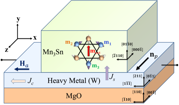
Figure 5: Spin-orbit torque device setup for manipulating the magnetic state in Mn₃Sn. The MgO substrate leads to tensile strain in the x-direction, and hence the PMA in Mn₃Sn. Spin-Hall effect in the heavy metal generates SOT when a charge current flows into it. $J_{c}$ and $J_{s}$ are the charge current density and the spin current density, respectively. $\mathbf{H}_{a}$ is the external magnetic field which is applied to aid the deterministic switching of the magnetic octupole, $\mathbf{m}_{\mathrm{oct}}$, in strained-Mn₃Sn.

To investigate the dynamics of Mn₃Sn under the effect of spin current, we consider the spin-Hall effect (SHE) setup shown in Fig. 5. This setup resembles the experimental designs from Refs. [19, 22], where Mn₃Sn grown epitaxially on a $(110)[001]$ MgO substrate exhibits uniaxial tensile strain in the x-direction with a PMA energy landscape [22, 29]. Hereafter, we only focus on the dynamics of single-domain Mn₃Sn with tensile strain while the discussion on the dynamics of Mn₃Sn with compressive strain is relegated to supplementary material. In our convention, as mentioned previously, the Kagome plane of Mn₃Sn is assumed to coincide with the x-y plane while the z-axis coincides with $[0001]$ direction. Charge-to-spin conversion in the heavy metal, due to the flow of charge current density, $J_{c}$, leads to the generation of a spin current density, $J_{s}$, polarized along ${\mathbf{n}}_{p}$, which is assumed to coincide with z-axis. Finally, the external field $\mathbf{H}_{a}$ is assumed to be applied along the x-direction, or $\varphi_{H}=180^{\circ}$.

For each sublattice of Mn₃Sn, the magnetization dynamics is governed by the classical Landau-Lifshitz-Gilbert (LLG) equation, which is a statement of the conservation of angular momentum. The LLG equations for the three sub-lattices are coupled via the exchange interactions [16, 32]. For sublattice $i$, the LLG equation is given as [41]

$$\begin{split}\dot{\mathbf{m}}_{i}&=-\gamma\quantity(\mathbf{m}_{i}\crossproduct\mathbf{H}_{i}^{\mathrm{eff}})+\alpha\quantity(\mathbf{m}_{i}\crossproduct\dot{\mathbf{m}}_{i})\\ &-\frac{\hbar}{2e}\frac{\gamma J_{s}}{M_{s}d_{a}}\mathbf{m}_{i}\crossproduct\quantity(\mathbf{m}_{i}\crossproduct\mathbf{n}_{p}),\end{split}$$ (4)

where $\dot{\mathbf{m}}_{i}=\partialderivative{\mathbf{m}_{i}}{t}$, $t$ is time in seconds, $\mathbf{H}_{i}^{\mathrm{eff}}$ is the effective magnetic field experienced by $\mathbf{m}_{i}$, $\alpha$ is the Gilbert damping parameter for Mn₃Sn, and $d_{a}$ is the thickness of the AFM layer. Other parameters in this equation, viz. $\hbar=1.054561\times 10^{-34}~{}\mathrm{J.s}$, $e=1.6\times 10^{-19}~{}\mathrm{C}$, and $\gamma=17.6\crossproduct 10^{10}~{}\mathrm{T^{-1}s^{-1}}$ are the reduced Planck’s constant, the elementary charge of an electron, and the gyromagnetic ratio, respectively. The spin current density depends on the input charge current density and the spin-Hall angle of the heavy metal (HM), $\theta_{\mathrm{SH}}$, as $J_{s}=\theta_{\mathrm{SH}}J_{c}$. The spin-Hall angle is associated with the efficiency of the SOT effect. Here, we consider the HM to be W since it has a large $\theta_{\mathrm{SH}}$ [18].

The effective magnetic field for sublattice $i$ can be obtained by using Eq. (1) as

$$\begin{split}\mathbf{H}_{i}^{\mathrm{eff}}&=-\frac{1}{M_{s}}\partialderivative{F}{\mathbf{m}_{i}}=-\frac{J_{E}}{M_{s}}\quantity(\mathbf{m}_{j}+\mathbf{m}_{k})\\ &+\frac{D_{M}\mathbf{z}\crossproduct\quantity(\mathbf{m}_{j}-\mathbf{m}_{k})}{M_{s}}+\frac{2K_{e}}{M_{s}}\quantity(\mathbf{m}_{i}\dotproduct\mathbf{u}_{e,i})\mathbf{u}_{e,i}+\mathbf{H}_{a},\end{split}$$ (5)

where $(i,j,k)=(1,2,3),(2,3,1),$ or $(3,1,2)$, respectively. For all the numerical results presented in this work, Eqs. (4) and (5) are solved simultaneously, for a range of external magnetic fields and input current density, with $\varphi_{\mathrm{oct}}=\pi/2$ as the initial state. On the other hand, if $\varphi_{\mathrm{oct}}=3\pi/2$ was chosen as the initial state, and the direction of magnetic field or that of the input current was reversed, exactly same conclusions would be drawn [22].

Numerical results of the steady state of the order parameter ($\mathbf{m}_{\mathrm{oct}}$) are presented in Fig. 6 for a range of $H_{0}$ and $J_{s}$ values. These results reveal that, for a non-zero magnetic field, the final state of $\mathbf{m}_{\mathrm{oct}}$ depends on the magnitude of the input spin current density with respect to two threshold currents—$J_{s}^{\mathrm{th1}}$ and $J_{s}^{\mathrm{th2}}$. If the injected current density is smaller than the lower threshold current, that is $J_{s}<J_{s}^{\mathrm{th1}}$, the ground state of the AFM evolves to a non-equilibrium stationary steady-state in the initial energy-well. On the other hand, if $J_{s}^{\mathrm{th1}}<J_{s}<J_{s}^{\mathrm{th2}}$ the order parameter deterministically switches to a non-equilibrium stationary steady-state in the other energy-well. Finally, when $J_{s}^{\mathrm{th2}}<J_{s}$ the octupole moment exhibits steady-state chiral oscillations, whose frequency could be tuned from the 100’s of MHz to the GHz range by varying $J_{s}$. The three regimes of operation are marked as N, S, and R for no switching, deterministic switching, and chiral-rotation, respectively. The overlaid dashed white lines represent $J_{s}^{\mathrm{th1}}$ and $J_{s}^{\mathrm{th2}}$. It can be observed that $J_{s}^{\mathrm{th1}}$ decreases with an increase in $H_{0}$ while $J_{s}^{\mathrm{th2}}$ increases with $H_{0}$. As a result, the range of input currents where the system exhibits deterministic switching increases with $H_{0}$. In the limiting case of $H_{0}=0$, $J_{s}^{\mathrm{th1}}=J_{s}^{\mathrm{th2}}$ and we do not observe any deterministic switching event. Instead, the order parameter displays either a non-equilibrium stationary state in the initial well or chiral oscillations. Similar results have been presented in Ref. [22].

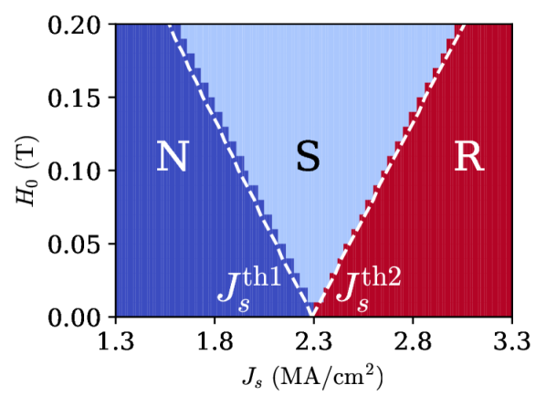
Figure 6: Final steady state as a function of the input current $J_{s}$ for different applied magnetic fields $H_{0}$. N, S, R represent no switching, switching, and chiral rotation, respectively. The dashed white lines represent the two threshold currents, $J_{s}^{\mathrm{th1}}$ and $J_{s}^{\mathrm{th2}}$ obtained from numerical solution of Eq. (7).

IV.1 Stationary State and Threshold Current

To explore the dependence of the dynamics on the intrinsic energy scale of the system, obtain analytic expressions for the two threshold currents as a function of the applied magnetic field and material parameters, and establish scaling laws related to switching and chiral oscillations, we evaluate the rate of change of the average magnetization, $\dot{\mathbf{m}}=\frac{\quantity(\dot{\mathbf{m}}_{1}+\dot{\mathbf{m}}_{2}+\dot{\mathbf{m}}_{3})}{3}$, as

$$\begin{split}\dot{\mathbf{m}}&=\frac{1}{3}\sum_{i=1}^{3}\bigg{(}-\gamma\quantity(\mathbf{m}_{i}\crossproduct\mathbf{H}_{i}^{\mathrm{eff}})+\alpha\quantity(\mathbf{m}_{i}\crossproduct\dot{\mathbf{m}}_{i})\Bigg{.}\\ &\left.-\frac{\hbar}{2e}\frac{\gamma J_{s}}{M_{s}d_{a}}\quantity(\mathbf{m}_{i}\crossproduct\quantity(\mathbf{m}_{i}\crossproduct\mathbf{z}))\right).\end{split}$$ (6)

where $\mathbf{m}_{i}\crossproduct\mathbf{H}_{i}^{\mathrm{eff}}=\frac{1}{3\mu_{0}M_{s}}\partialderivative{F}{\varphi_{\mathrm{oct}}}\mathbf{z}$ and Eq. (2) with $\varphi_{H}=\pi$ is used to evaluate $\partialderivative{F}{\varphi_{\mathrm{oct}}}$.

In the stationary states, the net torque on the order parameter is zero since the torque due to the internal and external magnetic fields is balanced by the spin-orbit torque. Part of the energy pumped into the system by the spin current is dissipated by the intrinsic damping of the system, and as a result the net input energy is lower than that required to overcome the energy barrier of the system shown in Fig. 4. Since the barrier height changes with the external magnetic field while the net input energy changes with the input current, the stationary steady-state is a function of both $H_{0}$ and $J_{s}$, as shown in Fig. 6. To get a precise value of these stationary states, firstly, we set the time derivatives to zero in Eq. (6). Secondly, we noticed from our numerical simulations that the z-components of all the sublattice vectors were zero in the stationary steady state; therefore, we set $m_{i,z}=u_{i}=0$ in Eq. (6) to arrive at the torque balance equation:

$$\begin{split}A\sin{\quantity(2\varphi_{\mathrm{oct}})}+B\sin{\quantity(6\varphi_{\mathrm{oct}})}-M_{s}H_{0}\quantity(C+D)\sin{\quantity(\varphi_{\mathrm{oct}})}\\ =\frac{\hbar}{2e}\frac{J_{s}}{d_{a}}.\end{split}$$ (7)

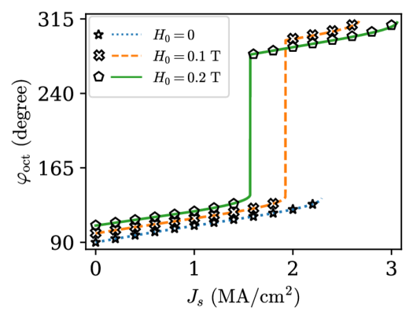
Figure 7: Stationary steady-states as a function of the applied spin current, $J_{s}$, for a thin film of Mn₃Sn under tensile strain. Numerical result from the solution of Eq. (4) (symbols) agree very well with the results obtained from Eq. (7) (lines)

For $0\leq J_{s}<J_{s}^{\mathrm{th1}}$, the solution of Eq. (7) should lead to one stationary solution with $\mathrm{GS}_{1}\leq\varphi_{\mathrm{oct}}<\pi$, where $\mathrm{GS}_{1}\in(\pi/2,\pi)$ is the smaller of the two minima of Eq. (2). On the other hand, when $J_{s}$ is increased above $J_{s}^{\mathrm{th1}}$, such that $J_{s}^{\mathrm{th1}}\leq J_{s}<J_{s}^{\mathrm{th2}}$, the order parameter should switch to a stationary state in the other well, and the solution of Eq. (7) should lead to $\mathrm{GS}_{2}<\varphi_{\mathrm{oct}}<2\pi$. Here, $\mathrm{GS}_{2}\in(\pi,3\pi/2)$ is the larger of the two minima of Eq. (2). Indeed the same can be observed from Fig. 7, where the numerical solutions of the coupled LLG equations (symbols) fit the solutions from Eq. (7) (lines) very well in both the wells, for three different values of $H_{0}$. Consequently, $J_{s}^{\mathrm{th1}}$ is the minimum current for which Eq. (7) has no solution in $(\mathrm{GS}_{1},\pi)$, but has a solution in $(\mathrm{GS}_{2},2\pi)$. On the other hand, $J_{s}^{\mathrm{th2}}$ is the minimum current for which Eq. (7) has no solutions. The numerical solution of the threshold currents for different $H_{0}$, obtained from Eq. (7), is shown by the dashed white lines overlaid on Fig. 6. It can be observed that the solutions from Eq. (7) match the results from Eq. (4) very well.

An exact expression of either of the threshold currents is cumbersome to obtain, however, for $H_{0}\ll\frac{2K_{e}J_{E}\delta_{E}}{M_{s}\quantity(K_{e}+J_{E}\delta_{E})}$ $(\approx 0.342~{}\mathrm{T}$ for the material parameters chosen in this paper), they can be approximated as

$$J_{s}^{\mathrm{th1}} =d_{a}\frac{2e}{\hbar}\quantity(-A+B-\frac{M_{s}H_{0}}{\sqrt{2}}\quantity(C+D)),$$ (8a)

$$J_{s}^{\mathrm{th2}} =d_{a}\frac{2e}{\hbar}\quantity(-A+B+\frac{M_{s}H_{0}}{\sqrt{2}}\quantity(C+D)).$$ (8b)

In the absence of a magnetic field, the threshold current corresponds to the $J_{s}$ which leads to $\varphi_{\mathrm{oct}}=135^{\circ}$ as $\sin{\quantity(2\varphi_{\mathrm{oct}})}=-1$ while $\sin{\quantity(6\varphi_{\mathrm{oct}})}=1$. We find that for small magnetic fields $\varphi_{\mathrm{oct}}$ is still close to $135^{\circ}$ at the threshold currents; therefore we approximate $J_{s}^{\mathrm{th1}}$ by using $\varphi_{\mathrm{oct}}=135^{\circ}$ in Eq. (7). To approximate $J_{s}^{\mathrm{th2}}$, we use $\varphi_{\mathrm{oct}}=315^{\circ}$ in Eq. (7). Figure 8 compares these analytic expressions (lines) against the values of the threshold currents obtained from the solution of Eq. (7) (symbols), for different values of $H_{0}$. The analytic results of Eq. (8) match very well against the numerical values. Although the error between the numerical and the analytic values of the two threshold currents increases with an increase in $H_{0}$, it is still smaller than $5\%$ even for $H_{0}=0.3~{}\mathrm{T}$. This linear dependence of the threshold current on the external field is similar to that in the case of a PMA ferromagnet driven by a SOT [42].

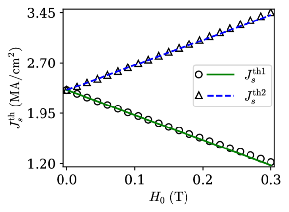
Figure 8: Comparison of the analytic expressions of threshold currents (Eq. (8)), shown by lines, against the numerical values obtained from the solution of Eq. (7), represented by symbols. The numerical and analytic values show excellent agreement for the values of $H_{0}$ considered here.

IV.2 Deterministic Switching Dynamics

For $H_{0}>0$ and $J_{s}^{\mathrm{th1}}\leq J_{s}<J_{s}^{\mathrm{th2}}$, the order parameter overcomes the barrier imposed by the effective intrinsic anisotropy and the external field at $\varphi_{\mathrm{oct}}=180^{\circ}$, shown in Fig. 4, and switches to the other well. This is because the net input energy due to the SOT is higher than the energy barrier height at $\varphi_{\mathrm{oct}}=180^{\circ}$. This energy, however, is smaller than the energy barrier at $\varphi_{\mathrm{oct}}=360^{\circ}$, and therefore, the order parameter is confined to the second well. If the input current was reversed for the same direction of $H_{0}$, the order parameter would go back to the initial well by overcoming the barrier at $\varphi_{\mathrm{oct}}=180^{\circ}$. On the other hand, if the magnetic field was reversed for the same direction of $J_{s}$, the order parameter would go back to the initial well by overcoming the barrier at $\varphi_{\mathrm{oct}}=360^{\circ}$. This bidirectional switching along with the low threshold currents and the sub-ns switching speed, as shown in Fig. 9, makes Mn₃Sn a prospective candidate for the next-generation magnetic memory devices. Here, the switching time, $t_{\mathrm{sw}}$, is defined as the time taken by the magnetic octupole to go from $\varphi_{\mathrm{oct}}=\pi/2$ to $\varphi_{\mathrm{oct}}=\pi$. It can be observed from Fig. 9 that $t_{\mathrm{sw}}$ decreases with an increase in either $J_{s}$ or $H_{0}$. For a fixed $H_{0}$, $t_{\mathrm{sw}}$ decreases with an increase in $J_{s}$ since a higher input current pumps in more energy into the system. On the other hand, at a fixed $J_{s}$, $t_{\mathrm{sw}}$ decreases with an increase in $H_{0}$ as the barrier height decreases.

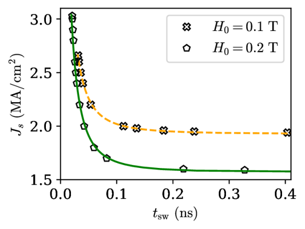
Figure 9: Switching time, $t_{\mathrm{sw}}$, as a function of the applied spin current, $J_{s}$, and external magnetic field, $H_{0}$, for a thin film of Mn₃Sn under tensile strain. In each case, the applied current is above $J_{s}^{\mathrm{th1}}$ and below $J_{s}^{\mathrm{th2}}$. $t_{\mathrm{sw}}$ obtained from the solution of Eq. (9) (lines) fits the data obtained from the solution of Eq. (4) (symbols) very well.

During the switching process, the time derivatives in Eq. (6) are non-zero, and so is each $u_{i}$. However, each $u_{i}$ as well as $m_{z}$ are small; therefore, the switching time can be obtained from the z-component of Eq. (6) as

$$\begin{split}&t_{\mathrm{sw}}=\frac{\alpha M_{s}}{\gamma}\frac{2e}{\hbar}\frac{d_{a}}{J_{s}}\int_{\pi/2}^{\pi}\\ &\times\frac{d\varphi_{\mathrm{oct}}^{{}^{\prime}}}{1-\frac{\quantity(A\sin{\quantity(2\varphi_{\mathrm{oct}}^{{}^{\prime}})}+B\sin{\quantity(6\varphi_{\mathrm{oct}}^{{}^{\prime}})}-M_{s}H_{0}\quantity(C+D)\sin{\quantity(\varphi_{\mathrm{oct}}^{{}^{\prime}})})}{\frac{\hbar}{2e}\frac{J_{s}}{d_{a}}}},\end{split}$$ (9)

where we have neglected the rate of change of $m_{z}$ since $\partialderivative{m_{z}}{t}\ll\alpha\partialderivative{\varphi_{\mathrm{oct}}}{t}$. It can be observed from Fig. 9 that the switching times obtained from the numerical integration of Eq. (9) (lines) fit the data obtained from the solution of Eq. (4) (symbols) very well, for the two different magnetic fields considered here.

IV.3 Oscillation Dynamics

For $H_{0}>0$ and $J_{s}^{\mathrm{th2}}\leq J_{s}$, the order parameter oscillates around the z-axis. This is because the net energy absorbed by the order parameter, which is the difference between the energy pumped into the system due to the SOT and the energy lost due to the intrinsic damping, is now higher than the energy barrier at $\varphi_{\mathrm{oct}}=360^{\circ}$ shown in Fig. 4. Consequently, the order parameter oscillates between the two wells with frequencies ranging from 100’s of MHz to GHz as shown in Fig. 10. It can be observed from Fig. 10 that for large input currents ($J_{s}\gg J_{s}^{\mathrm{th2}}$), the oscillation frequency, $f$, is almost independent of $H_{0}$ and increases linearly with $J_{s}$. The dash-dotted red line, which corresponds to $f=\frac{\gamma}{2\pi\alpha M_{s}}\frac{\hbar}{2e}\frac{J_{s}}{d_{a}}$, represents this behavior clearly. For such large $J_{s}$, the z-component of the sublattice vectors, $u_{i}$, increases and the effect of the uniaxial anisotropy and $H_{0}$ on the dynamics becomes negligible. For $J_{s}\simeq J_{s}^{\mathrm{th2}}$, on the other hand, $f$ increases non-linearly with an increase in $J_{s}$ since the dynamics is strongly influenced by the effective anisotropy. In addition, in the non-linear regime, higher $H_{0}$ leads to lower $f$, at a fixed $J_{s}$, as depicted clearly in the inset of Fig. 10. This is because the barrier height at $\varphi_{\mathrm{oct}}=360^{\circ}$ increases with an increase in $H_{0}$, thereby requiring higher input energy in order to achieve the same oscillation frequency. Unlike the switching dynamics, the current-driven oscillations are accompanied by a significant out-of-(Kagome)-plane component of the order parameter, which leads to an exchange field along the z-direction. However, such an exchange energy interaction is not included in Eq. (2), and consequently in Eq. (6). Therefore, our model cannot be cannot be used to obtain a unified model of $f$ as a function of $H_{0}$ and $J_{s}$.

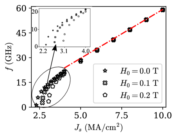
Figure 10: Oscillation frequency as a function of the applied spin current, $J_{s}$, and external magnetic field, $H_{0}$, for a thin film of Mn₃Sn under tensile strain. In each case, the applied current is above the respective $J_{s}^{\mathrm{th2}}$. The dash-dotted red line represents $f=\frac{\gamma}{2\pi\alpha M_{s}}\frac{\hbar}{2e}\frac{J_{s}}{d_{a}}$ and fits the numerical data very well for large $J_{s}$. The figure in the inset shows the variation in $f$ with $J_{s}$ for smaller input currents.

V Effect of Damping

The results presented in this work, so far, correspond to a Gilbert damping constant of $\alpha=0.003$, which has previously been used for numerical analysis in Refs. [29, 26]. On the other hand, a lower damping constant of $\alpha=0.0007$ was used in other recent works [20, 22]. In particular in Ref. [22], it was shown through numerical simulations that for $\alpha=0.0007$, as compared to $\alpha=0.003$, the lower limit of external magnetic field for deterministic switching was a non-zero value. That is, for low values of $H_{0}\gtrsim 0$, the order parameter cannot be deterministically switched. Instead, the order parameter exhibits either a stationary steady-state or chiral oscillation depending on the magnitude of the input current. This behavior is distinct from that presented in Figs. 6 and 8. Therefore, we numerically investigate the dependence of the final steady states and the threshold currents on $\alpha$.

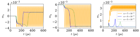
Figure 11: The three components of the average magnetization, $\mathbf{m}$, as a function of time for three different values of the Gilbert damping constant, $\alpha$. Here, $H_{0}=0.1~{}\mathrm{T}$ and $J_{s}=2~{}\mathrm{MA/cm^{2}}$ are both applied to the equilibrium state of Fig. 2(c) at $t=100~{}\mathrm{ps}$. In the case of $\alpha=0.003$ and $0.005$ the magnetic octupole moment switches to the same final steady state in the other well. Switching time increases with $\alpha$. On the other hand, for $\alpha=0.0007$, chiral oscillations with large $m_{z}$ are observed.

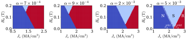
Figure 12: Final steady state as a function of the input current $J_{s}$ and applied magnetic fields for different Gilbert damping constant. Here, N, S, R represent no switching, switching, and chiral rotation, respectively. The white dashed lines superimposed on the phase space are the two threshold currents, as discussed in the case of $\alpha=3\times 10^{-3}$.

Figure 11 shows the three components of the average magnetization vector, $\mathbf{m}$, for different values of $\alpha$ but the same values of $H_{0}$ and $J_{s}$. In the case of $\alpha=5\times 10^{-3}$, for $J_{s}=2~{}\mathrm{MA/cm^{2}}$ and $H_{0}=0.1~{}\mathrm{T}$ applied at $t=100~{}\mathrm{ps}$, the AFM magnetization switches to a steady state in the other well. This is signified by a change in the sign of $m_{y}$. As shown by the dashed blue curve and dotted green curve, the final steady state for $\alpha=5\times 10^{-3}$ is exactly same as that obtained for $\alpha=3\times 10^{-3}$. The switching time, however, is longer in the case of higher damping since $t_{\mathrm{sw}}$ is directly proportional to $\alpha$ (Eq. (9)). On the other hand, for the case of lower damping, namely $\alpha=7\times 10^{-4}$, the order parameter exhibits chiral rotations when $J_{s}=2~{}\mathrm{MA/cm^{2}}$ and $H_{0}=0.1~{}\mathrm{T}$ are applied at $t=100~{}\mathrm{ps}$. This suggests that for lower damping, the threshold currents are lower than those predicted by Eq. (8); and could be dependent on $\alpha$. It can also be observed that for $\alpha=7\times 10^{-4}$, the oscillating $m_{z}$ is rather large. This suggests that the out-of-(Kagome)-plane exchange interaction plays a major role in the oscillation dynamics, similar to that discussed in Section IV.3.

To further elucidate this dependence of the dynamics on $\alpha$, we present the final steady states as a function of $J_{s}$ and $H_{0}$ for different values of $\alpha$, as shown in Fig. 12. It can be observed that for the lower values of $\alpha$, the final steady states and the threshold currents are indeed dependent on damping. Although both the threshold currents seem to scale linearly with $H_{0}$ for $\alpha\leq 2\times 10^{-3}$, it can be clearly observed that they depend on the Gilbert damping constant, unlike Eq. (8). Moreover, for low values of $H_{0}$, deterministic switching is not possible; instead the order parameter can only exhibit oscillation dynamics above the threshold current. It is observed that deterministic switching between the two stable states of Mn₃Sn becomes feasible again for larger values of $H_{0}$. This lower limit of $H_{0}$ for deterministic switching dynamics decreases as $\alpha$ increases. Further investigation is required to understand this dependence of the dynamics on the damping and is beyond the scope of the present work. On the other hand, we find that for $\alpha=5\times 10^{-3}$ the analysis presented in Section IV holds true.

VI Conclusion

Mn₃Sn is a metallic antiferromagnet that shows large AHE, ANE, and MOKE signals. In addition, the octupole states can be detected via TMR in an all-antiferromagnetic tunnel junction comprising two layers of Mn₃Sn with an insulator layer sandwiched between them. Bulk Mn₃Sn has a $120^{\circ}$ anti-chiral structure, however, a competition between the local anisotropy and the DMI leads to the existence of a small net magnetization which is six-fold degenerate. Application of strain to bulk Mn₃Sn reduces its symmetry from six-fold to two-fold degenerate, and provides a way to control the strength of the net magnetization as well as that of the AHE signal. In this work, we analyzed the case of both uniaxial compressive and tensile strains, and discussed the dependence of the magnetic octupole on the strain as well as on the external field. Since recent experiment reported tensile strain in epitaxial Mn₃Sn grown on (110)[001] MgO substrate, we numerically and analytically explored the field-assisted SOT driven dynamics in monodomain Mn₃Sn with tensile strain. We found that the order parameter exhibits either a stationary state or chiral oscillations in the absence of a symmetry-breaking field. On the other hand, when an external field is applied, in addition to the stationary state and chiral oscillations, the order parameter can also be deterministically switched between the two stable states for a range of currents. We derived an effective equation which accurately predicts the stationary states in both the wells. We also derived simple analytic expressions of the threshold currents and found them to agree very well against the numerical results for small external magnetic fields. We obtained functional form of the switching time as a function of the material parameters and the external stimuli and found it to match very well against numerical data. The frequency of chiral oscillations, which can be tuned from 100’s of MHz to GHz range, was found to vary non-linearly closer to the threshold current and linearly for larger input currents. Further, through numerical simulations, we showed that the order dynamics is dependent on the Gilbert damping for lower values of $\alpha$. For the sake of a complete picture, we also explored the field-assisted switching dynamics in thin films of Mn₃Sn with compressive strain, and presented the relevant results in the supplementary document. We expect the insights of our theoretical investigation to be useful to both theorists and experimentalists in their exploration of the interplay of field-assisted SOT and the order dynamics in Mn₃Sn, and further benchmarking the device performance.

Supplementary Material

See supplementary material for the perturbative analysis of the ground state, the SOT-driven dynamics of thin films of Mn₃Sn with compressive strain, and a brief discussion of the AHE and TMR detection schemes.