Thermodynamics of spin-$1/2$ fermions on coarse temporal lattices
using automated algebra

Abstract

Recent advances in automated algebra for dilute Fermi gases in the virial expansion, where coarse temporal lattices were found advantageous, motivate the study of more general computational schemes that could be applied to arbitrary densities, beyond the dilute limit where the virial expansion is physically reasonable. We propose here such an approach by developing what we call the Quantum Thermodynamics Computational Engine (QTCE). In QTCE, the imaginary-time direction is discretized and the interaction is accounted for via a quantum cumulant expansion, where the coefficients are expressed in terms of noninteracting expectation values. The aim of QTCE is to enable the systematic resolution of interaction effects at fixed temporal discretization, as in lattice Monte Carlo calculations, but here in an algebraic rather than numerical fashion. Using this approach, in combination with numerical integration techniques (both known and alternative ones proposed here), we explore the thermodynamics of spin-$1/2$ fermions, focusing on the unitary limit in 3 spatial dimensions, but also exploring the effects of continuously varying the spatial dimension below 3. We find that, remarkably, extremely coarse temporal lattices, when suitably renormalized using known results from the virial expansion, yield stable partial sums for QTCE’s cumulant expansion which are qualitatively and quantitatively correct in wide regions, compared with known experimental results.

I Introduction

Approaches to the quantum many-body problem, in particular at finite temperature, can be roughly divided into two large classes: analytical methods (e.g. perturbation theory, mean-field approaches, etc) and numerical methods (e.g. all the well-known flavors of quantum Monte Carlo; see e.g. [1, 2]). Naturally, the former do require some numerical evaluation at the very end, while the latter do require some analytic development (i.e. rewriting the problem in a way amenable to modern computers) before any actual numerical computations are carried out.

As modern computers stay on the path set by Moore’s law, interesting approaches have emerged that bridge between the above two paradigms. This is the idea of automated algebra: the use of computers to perform extremely lengthy derivations (of a scale that would be impossible to accomplish by hand in a human lifetime) in order to explore the quantum many-body problem analytically as far as possible, before proceeding to numerical evaluation at the end. The application of this concept has seen examples in nuclear physics (see e.g. [3, 4, 5, 6]) and quantum chemistry (see e.g. [7]) for some time and more recently in ultracold fermions (see below). One may regard the idea of automated algebra as merely extending conventional analytic methods, which is correct in some regard but we have found, in the research presented here and elsewhere, that conventional numerical approaches also inform automated algebra methods in relevant and useful ways.

As a specific example pursued by our group, automated algebra has successfully pushed the boundaries of the quantum virial expansion (VE) for spin-$1/2$ Fermi gases in a wide range of settings (see e.g. [8, 9, 10] and [11] for a recent review), managing to obtain precise estimates of up to the fifth order coefficient. Encouraged by the success of automated algebra for the VE, here we explore a different route that is not a priori restricted to low-density regimes. We propose an approach that we call the Quantum Thermodynamics Computational Engine (QTCE) whereby the imaginary-time direction is discretized and the interaction effects are accounted for via a quantum cumulant expansion. In turn, the quantum cumulants at a given order are calculated using the corresponding moments (and their lower-order counterparts) in terms of noninteracting expectation values. In its present form, the objective of QTCE is to enable the calculation of fundamental thermodynamic quantities such as the pressure, density, and isothermal compressibility, in a systematic resolution of interaction effects at fixed temporal discretization. As in our previous VE investigations, we focus on short-range, contact interactions, such that the matrix elements have no momentum dependence (aside from total momentum conservation, of course), which facilitates the exploration of novel approaches to the evaluation of the relevant multidimensional integrals using algebraic methods.

The remainder of this paper is organized as follows. Section II introduces the Hamiltonian of our system with details of the discretization and outlines the expansion of the partition function in terms of multivariate quantum cumulants. Section III then connects this expansion with the noninteracting generating functional of density correlation functions before describing the QTCE implementation. Section IV presents our thermodynamic results for spin-1/2 fermions, focusing on the universal limit of the unitary Fermi gas. In Sec. V we discuss two systematic effects related to coarse temporal lattices and the choice of integrator approach. Finally, we conclude in Sec. VI, where we also comment on the generalizability of our method.

II Formalism

II.1 Model, partition function, and discretization

We consider a non-relativistic, spin-$1/2$ fermionic system with Hamiltonian $\hat{H}=\hat{T}+\hat{V}$, where

$$\hat{T}=\sum_{s=\uparrow,\downarrow}\int d^{d}x\text{ }\hat{\psi}_{s}^{\dagger}({\bf x})\left(-\frac{\hbar^{2}\nabla^{2}}{2m}\right)\hat{\psi}_{s}({\bf x}),$$ (1)

is the kinetic energy in terms of spatial dimension $d$, particle mass $m$, and field operators $\hat{\psi}_{s}^{\dagger}$, $\hat{\psi}_{s}$ for spin $s$, and

$$\hat{V}=-g\int d^{d}x\text{ }\hat{n}_{\uparrow}({\bf x})\hat{n}_{\downarrow}({\bf x}),$$ (2)

is a contact interaction with coupling constant $g$ and particle density operators $\hat{n}_{s}=\hat{\psi}_{s}^{\dagger}\hat{\psi}_{s}$. To proceed, we let $\hbar=k_{B}=m=1$ and regularize the interaction by discretizing spacetime using a spatial lattice spacing $\ell$ such that the potential energy takes the form

$$\hat{V}=-g_{lat}\sum_{\bf x}\hat{n}_{\uparrow}({\bf x})\hat{n}_{\downarrow}({\bf x}),$$ (3)

where the operators are now dimensionless and $g_{lat}=g/\ell^{d}$.

To study thermodynamics, the central quantity of interest is the grand-canonical partition function of the unpolarized, interacting system,

$$\mathcal{Z}=\text{Tr}\left[e^{-\beta(\hat{H}-\mu\hat{N})}\right],$$ (4)

where $\beta$ is the inverse temperature, $\mu$ is the chemical potential (common to both spin degrees of freedom, as we focus on unpolarized matter here), and $\hat{N}$ is the total particle number.

The central challenging point of quantum thermodynamics is that $\hat{T}$ and $\hat{V}$ do not commute. To address that problem, we follow a common route and introduce a temporal discretization $\beta=\tau N_{\tau}$ where $N_{\tau}$ is a positive integer and $\tau$ is the spacing, which allows us to separate the kinetic and potential energy exponential factors via a (symmetric) Trotter-Suzuki factorization, namely

$$e^{-\tau(\hat{H}-\mu\hat{N})}=e^{-\tau\hat{K}_{0}/2}e^{-\tau\hat{V}}e^{-\tau\hat{K}_{0}/2}+O(\tau^{3}),$$ (5)

where $\hat{K}_{0}=\hat{T}-\mu\hat{N}$. The net result on the partition function is the following approximation (valid up to $O(\tau^{2})$ once all $N_{\tau}$ time slices are accounted for):

$$\mathcal{Z}=\text{Tr}\left[e^{-\beta(\hat{H}-\mu\hat{N})}\right]\simeq\text{Tr}\left[e^{-\tau\hat{K}_{0}}e^{-\tau\hat{V}}e^{-\tau\hat{K}_{0}}e^{-\tau\hat{V}}\dots\right],$$ (6)

where there are $N_{\tau}$ factors. Since $\tau=\beta/N_{\tau}$, it follows that increasing $N_{\tau}$ improves the accuracy of the final answer while also increasing the computational cost.

On a spatial lattice, we may use the property $\hat{n}^{2}=\hat{n}$, valid for dimensionless, lattice fermion density operators, to write

$$e^{-\tau\hat{V}} = \prod_{\bf x}\left[1+C\hat{n}_{\uparrow}({\bf x})\hat{n}_{\downarrow}({\bf x})\right]$$ (7)

$$= \sum_{k}\frac{\lambda^{k}}{k!}\hat{V}_{k},$$ (8)

for $k\geq 0$ where we have introduced an arbitrary parameter $\lambda$ (see below) and

$$\hat{V}_{k}=C^{k}\sum_{{\bf x}_{1}\neq{\bf x}_{2}\neq\dots\neq{\bf x}_{k}}\hat{n}_{2}({\bf x}_{1})\hat{n}_{2}({\bf x}_{2})\dots\hat{n}_{2}({\bf x}_{k}),$$ (9)

with $C=(e^{\tau g}-1)/\lambda$, $\hat{n}_{2}({\bf x})=\hat{n}_{\uparrow}({\bf x})\hat{n}_{\downarrow}({\bf x})$, and $\hat{V}_{0}=\openone$. When envisioning taking the large-$N_{\tau}$ limit at constant $\beta$, it is useful to set $\lambda=1/N_{\tau}$, such that, in that limit, one has $C\to\beta g$, i.e. $C$ approaches a well-defined limit in terms of the parameters of the theory. In practice, $C$ is set by renormalization (more on this below), such that the choice of $\lambda$ should be immaterial (up to, possibly, numerical artifacts). We will also see below that choosing $\lambda=1/N_{\tau}$ makes sense from the point of view of the scaling of the number of terms in the cumulant expansion presented below as $N_{\tau}$ is increased.

II.2 Moment and cumulant expansions

We make use of the interaction expansion of Eq. (7) by expanding the partition function into a quantum moment expansion:

$$\frac{\mathcal{Z}(\lambda)}{\mathcal{Z}_{0}}=\sum_{\{n\}=0}^{\infty}\frac{\lambda^{n_{1}+n_{2}+\dots+n_{N_{\tau}}}}{n_{1}!n_{2}!\dots n_{N_{\tau}}!}W_{n_{1},n_{2},\dots,n_{N_{\tau}}},$$ (10)

where $\mathcal{Z}_{0}$ is the partition function of the non-interacting system and

$$W_{n_{1},n_{2},\dots,n_{N_{\tau}}} = \frac{1}{\mathcal{Z}_{0}}\text{Tr}\left[e^{-\tau\hat{K}_{0}}\hat{V}_{n_{1}}e^{-\tau\hat{K}_{0}}\hat{V}_{n_{2}}\dots\right],$$

are the quantum moments. Based on the above moment expansion, the following cumulant expansion results, which is one of the cornerstones of the QTCE, as described below:

$$\ln\left(\frac{\mathcal{Z}(\lambda)}{\mathcal{Z}_{0}}\right)=\sum_{\{n\}=0}^{\infty}\frac{\lambda^{n_{1}+n_{2}+\dots+n_{N_{\tau}}}}{n_{1}!n_{2}!\dots n_{N_{\tau}}!}\kappa_{n_{1},n_{2},\dots,n_{N_{\tau}}},$$ (12)

where $\kappa_{0,0,\dots,0}=0$ for any value of $N_{\tau}$, because $W_{0,0,\dots,0}=1$ for all $N_{\tau}$. It is this expansion that gives us access to thermodynamic observables via the fundamental relation

$$\beta(P-P_{0})V=\ln\left(\frac{\mathcal{Z}}{\mathcal{Z}_{0}}\right),$$ (13)

where ($P_{0}$) $P$ is the pressure of the (non-)interacting system and $V$ is the $d$-dimensional volume.

The series form of Eq. (12) naturally allows one to study the effect of including successively higher-order terms, when the series is truncated at some order $N_{\kappa}$. Thus, our method has two parameters, namely $N_{\tau}$ and $N_{\kappa}$, which can be systematically increased. In this work, we favor increasing $N_{\kappa}$ while keeping $N_{\tau}$ relatively small (thus the “coarse temporal lattices” advertised in the title). Note that taking these limits in reverse order amounts to a perturbative approach, while increasing $N_{\kappa}$ first, at constant $N_{\tau}$ (as we propose), is formally closer to lattice Monte Carlo calculations.

Using

$$\beta P_{0}V=\left(\frac{L}{\lambda_{T}}\right)^{d}I_{0}(z),$$ (14)

where $\lambda_{T}=\sqrt{2\pi\beta}$ is the thermal wavelength, and

$$I_{0}(z)=\frac{1}{(2\pi)^{d/2}}\int dx\ln(1+ze^{-\frac{x^{2}}{2}}),$$ (15)

we can reformulate Eq. (12) as

$$\frac{P}{P_{0}} = 1+\sum_{\{n\}=1}^{\infty}\lambda^{n_{1}+n_{2}+\dots+n_{N_{\tau}}}\frac{\bar{\kappa}_{n_{1},n_{2},\dots,n_{N_{\tau}}}}{n_{1}!n_{2}!\dots n_{N_{\tau}}!},$$ (16)

$$= 1+\lambda\bar{K}_{1}+\lambda^{2}\bar{K}_{2}+\dots,$$ (17)

where

$$\bar{\kappa}_{n_{1},n_{2},\dots,n_{N_{\tau}}}=\left(\frac{\lambda_{T}}{L}\right)^{d}\frac{\kappa_{n_{1},n_{2},\dots,n_{N_{\tau}}}}{I_{0}(z)},$$ (18)

and we define the “assembled cumulants” as

$$\bar{K}_{1} = \bar{\kappa}_{1,0,\dots,0}+\bar{\kappa}_{0,1,0,\dots,0}+\dots+\bar{\kappa}_{0,0,\dots,1},$$ (19)

$$\bar{K}_{2} = \frac{1}{2}\bar{\kappa}_{2,0,\dots,0}+\frac{1}{2}\bar{\kappa}_{0,2,0,\dots,0}+\dots$$ (20)

$$+\frac{1}{2}\bar{\kappa}_{0,0,\dots,2}+\bar{\kappa}_{1,1,0,\dots,0}+\dots,$$

and so on.

Note that since $\bar{\kappa}_{1,0,\dots,0}=\bar{\kappa}_{0,1,0,\dots,0}=\dots=\bar{\kappa}_{0,0,\dots,1}$, we can write $\bar{K}_{1}=N_{\tau}\bar{\kappa}_{1,0,\dots,0}$, which explicitly shows that $\bar{K}_{1}$ is linear in $N_{\tau}$, and this dependence is then cancelled in the expansion by the factor $\lambda=1/N_{\tau}$ in Eq. (17). Similarly, it is easy to see that there are $\propto N^{2}_{\tau}$ terms in $\bar{K}_{2}$, whose number is balanced by the $\lambda^{2}=1/N^{2}_{\tau}$ dependence in Eq. (17). The same reasoning applies to all orders in the expansion of Eq. (17).

These $\bar{K}_{n}$ quantities are useful for analyzing the system and are the main output of QTCE, which returns results up to a given cumulant order $N_{\kappa}$, corresponding to the upper limit on the summation in Eq. (16). We expect the $\kappa_{n_{1},n_{2},\dots,n_{N_{\tau}}}$ to be extensive quantities proportional to $\left({L}/{\lambda_{T}}\right)^{d}$ and therefore all $\bar{\kappa}_{n_{1},n_{2},\dots,n_{N_{\tau}}}$ to be intensive.

The cumulants can generally be expressed in terms of the moments via recursive formulas, such that to calculate a cumulant at a given order, one needs all of the moments up to and including that order [12]. For example, for $N_{\tau}=1$,

$$\kappa_{n}=W_{n}-\sum_{m=1}^{n-1}C^{n-1}_{m-1}\kappa_{m}W_{(n-m)},$$ (21)

where $C^{n}_{k}=n!/(k!(n-k)!)$ is the binomial coefficient.

Since Eq. (13) establishes that $\ln(\mathcal{Z}/\mathcal{Z}_{0})$ is proportional to the volume $V$, and $V$ and $\lambda$ are independent variables, it must be that within each cumulant $\kappa_{n}$ the only terms that contribute are those with the proper spatial volume scaling $\propto V$. Since this is true for all $n$, we see that in Eq. (21) the role of the terms in the sum is to cancel out the unnecessary terms in $W_{n}$. In practice, we therefore proceed simply by calculating $W_{n}$ and retaining only the terms with linear $V$ scaling. In terms of Feynman diagrams, this amounts to keeping only the connected diagrams, as indicated by the linked-cluster theorem (see e.g. Ref. [13]). Thus, we are able to eliminate a large number of terms early on in the calculation, thereby reducing the computational cost.

III Computational details

III.1 Toward calculating the moments $W_{n_{1},n_{2},\dots,n_{N_{\tau}}}$ with generating functionals

In Eq. (II.2) we saw that in order to calculate the moment $W_{n_{1},n_{2},\dots,n_{N_{\tau}}}$ we need

$$\text{Tr}\left[e^{-\tau\hat{K}_{0}}\hat{V}_{n_{1}}e^{-\tau\hat{K}_{0}}\hat{V}_{n_{2}}\dots\right]=$$

$$\int\mathcal{D}x\;\text{Tr}\left[e^{-\tau\hat{K}_{0}}\prod_{k=1}^{n_{1}}\hat{n}_{2}({\bf x}_{k})e^{-\tau\hat{K}_{0}}\prod_{k=1}^{n_{2}}\hat{n}_{2}({\bf y}_{k})\dots\right],$$

where we define

$$\int\mathcal{D}x\equiv\sum_{{\bf x}_{1}\neq\dots\neq{\bf x}_{n_{1}}}C^{n_{1}}\sum_{{\bf y}_{1}\neq\dots\neq{\bf y}_{n_{2}}}C^{n_{2}}\dots,$$ (23)

to represent the spatial integration that is part of the simplification and integration modules of QTCE.

Next, we turn to calculating the noninteracting expectation value

$$\frac{1}{\mathcal{Z}_{0}}\text{Tr}\left[e^{-\tau\hat{K}_{0}}\prod_{k=1}^{n_{1}}\hat{n}_{2}({\bf x}_{k})e^{-\tau\hat{K}_{0}}\prod_{k=1}^{n_{2}}\hat{n}_{2}({\bf y}_{k})\dots\right],$$ (24)

using a noninteracting generating functional and automated algebra.

III.2 Using the non-interacting generating functional of density correlation functions

The noninteracting generating functional of density correlation functions is defined as

$$\mathcal{Z}_{0}[j]=\text{Tr}\left[e^{-\tau\hat{K}_{0}}e^{\hat{V}_{\text{ext},1}}e^{-\tau\hat{K}_{0}}e^{\hat{V}_{\text{ext},2}}\dots e^{-\tau\hat{K}_{0}}e^{\hat{V}_{\text{ext},N_{\tau}}}\right],$$ (25)

where we couple our source $j({\bf x},t)$ to the density at each spacetime point via

$$\hat{V}_{\text{ext},t}=\sum_{\bf x}\,j({\bf x},t)\hat{n}({\bf x}),$$ (26)

which includes an imaginary-time coordinate $t$ to identify the various insertions of $e^{\hat{V}_{\text{ext}}}$ in $\mathcal{Z}_{0}[j]$. Furthermore, we have assumed that our system is placed on a lattice as a way to regularize a future interaction, such that all the quantities below, unless otherwise stated, are lattice quantities.

By taking functional derivatives of $\mathcal{Z}_{0}[j]$ with respect to $j$ at a given point in space and time, and then dividing by $\mathcal{Z}_{0}$, we can generate noninteracting expectation values of any combination of density operators. For example,

$$\left\langle\prod_{\bf x}\hat{n}({\bf x})\right\rangle_{0} = \frac{1}{\mathcal{Z}_{0}}\text{Tr}\left[e^{-\beta\hat{K}_{0}}\hat{n}({\bf x}_{1})\dots\hat{n}({\bf x}_{k})\right]$$ (27)

$$= \frac{1}{\mathcal{Z}_{0}}\left.\frac{\delta^{k}\mathcal{Z}_{0}[j]}{\delta j({\bf x}_{1},1)\dots\delta j({\bf x}_{k},1)}\right|_{j=0},$$

where the $1$ in $({\bf x},1)$ indicates the first time slice. By taking derivatives at different time slices, the above expression can be generalized to generate expectation values of the form in Eq. (24).

Because all the operators involved are now exponentials of one-body operators, the following essential simplification holds:

$$\mathcal{Z}_{0}[j] = \det(1+zU[j])$$ (28)

$$= \exp\tr\ln(1+zU[j]),$$

where $z=e^{\beta\mu}$ is the fugacity and $U=U_{1}U_{2}U_{3}\dots U_{N_{\tau}}$ is the product of the one-particle representation of the transfer matrices

$$[U_{t}]_{\bf pp^{\prime}} = \left\langle{\bf p}\right|e^{-\tau\hat{T}}e^{\hat{V}_{\text{ext},t}}\left|{\bf p^{\prime}}\right\rangle,$$ (29)

$$= e^{-\tau p^{2}/(2m)}\left\langle{\bf p}\right|e^{\hat{V}_{\text{ext},t}}\left|{\bf p^{\prime}}\right\rangle,$$

where $|{\bf p}\rangle$ are single-particle states and $t$ corresponds to the time slice.

It is not difficult to show (in fact, this is a standard result in many-body physics; see e.g. Refs. [13, 1]) that there is another useful representation for the generating functional, namely

$$\mathcal{Z}_{0}[j]=\det M[j],$$ (30)

where

$$M[j]=\begin{pmatrix}1&0&\cdots&U_{N_{\tau}}\\ -U_{1}&1&\cdots&0\\ 0&-U_{2}&\ddots&0\\ \vdots&\vdots&\ddots&\vdots\\ 0&\cdots&-U_{N_{\tau}-1}&1\end{pmatrix}.$$ (31)

We will refer to Eqs. (28) and (30) as the $U$ and $M$ representations, respectively, but they are often also referred to as the spatial and spacetime representations.

To simplify our notation below, we define

$$G(z)\equiv\frac{ze^{-\beta T}}{1+ze^{-\beta T}},$$ (32)

which is a matrix as $T$ is the single-particle matrix representation of $\hat{T}$, i.e.

$$[T]_{\bf pp^{\prime}}=\left\langle{\bf p}\right|\hat{T}\left|{\bf p^{\prime}}\right\rangle=\delta_{\bf pp^{\prime}}\frac{p^{2}}{2m}.$$ (33)

We also define

$$\mathcal{U}_{x_{1},x_{2},\dots,x_{n}}\equiv e^{+\beta T}\frac{\delta^{n}U}{\delta j(x_{1})\delta j(x_{2})\dots\delta j(x_{n})},$$ (34)

which is also a matrix, where $x_{k}=({\bf x}_{k},t_{k})$, and similarly

$$\mathcal{M}_{x_{1},x_{2},\dots,x_{n}}\equiv\frac{\delta^{n}M}{\delta j(x_{1})\delta j(x_{2})\dots\delta j(x_{n})}.$$ (35)

It is very easy to see from the above form of $M$ that any derivative of $M$ beyond the first one vanishes when evaluated at unequal times, i.e.

$$\mathcal{M}_{x_{1},x_{2}}\equiv 0,$$ (36)

for $t_{1}\neq t_{2}$ and arbitrary $j$.

Similarly, it is not difficult to see that, for $t_{1}=t_{2}$,

$$\mathcal{U}_{x_{1},x_{2}}\equiv 0,$$ (37)

for ${\bf x}_{1}\neq{\bf x}_{2}$ and arbitrary $j$, because both $\hat{V}_{\text{ext},t}$ and its exponential are diagonal matrices in coordinate space.

As usual when working with generating functionals, we set $j=0$ at the end of the calculation. With these definitions one finds, for example,

$$\langle\hat{n}(x_{1})\rangle_{0}=\tr\left[G\,\mathcal{U}_{x_{1}}\right]=\tr\left[M^{-1}\,\mathcal{M}_{x_{1}}\right],$$ (38)

and

$$\langle\hat{n}(x_{1})\hat{n}(x_{2})\rangle_{0} = \tr\left[M^{-1}\,\mathcal{M}_{x_{1}}\right]\tr\left[M^{-1}\,\mathcal{M}_{x_{2}}\right]$$ (39)

$$- \tr\left[M^{-1}\,\mathcal{M}_{x_{1}}\,M^{-1}\,\mathcal{M}_{x_{2}}\right]$$

$$+ \tr\left[M^{-1}\,\mathcal{M}_{x_{1},x_{2}}\right],$$

where the last term vanishes if $t_{1}\neq t_{2}$. In the $U$ representation, the above becomes

$$\langle\hat{n}(x_{1})\hat{n}(x_{2})\rangle_{0} = \tr\left[G\,\mathcal{U}_{x_{1}}\right]\tr\left[G\,\mathcal{U}_{x_{2}}\right]$$ (40)

$$- \tr\left[G\,\mathcal{U}_{x_{1}}\,G\,\mathcal{U}_{x_{2}}\right]$$

$$+ \tr\left[G\,\mathcal{U}_{x_{1},x_{2}}\right],$$

and so forth, where the traces are computed in momentum space for the homogeneous system. [In the above expressions, the time dependence appearing in the operators $\hat{n}$ simply indicates the time slice where they are to be inserted, in expressions such as Eq. (24).]

The case of equal times $t_{1}=t_{2}$ requires some care for general interactions, as it may generate terms that diverge in the continuum limit [namely the third term in the right-hand side of Eqs. (39) and (40)]. For a contact interaction, as is our interest here, those terms are simply not present, by virtue of Eq. (9), i.e. the required equal-time correlations are only needed at unequal spatial separation.

Thus, we see that to calculate the moments (and thus access the cumulants), one can begin by generating trace expressions for density correlations that simply involve the propagator of Eq. (32) and the first derivative of $U$. This is one of the first steps of the automated algebra code implemented by the QTCE. Note that at this stage, we have focused on two-body local interactions (i.e. of the density-density form); generalizations of the method are discussed in Section VI.

III.3 The Quantum Thermodynamics Computational Engine

The QTCE uses the above formalism and computational approach to evaluate the quantum cumulants of Eq. (12) following the steps outlined below.

1. Expectation value identification: Determine which expectation values need to be calculated. These correspond to Eq. (24) but at this stage are simply identified by the set of indices $\{n_{i}\}$.

2. Term generation: Generate expressions for the required non-interacting expectation values using functional derivatives. At the end of this step, we have expressions as in Eq. (40).

3. Simplification: Carry out coordinate sums of Eq. (23) as well as other simplifications before assembling the cumulants. The outputs of this step are multidimensional momentum integrals, each corresponding to a diagram. They have the general form

   $$\int{\mathcal{D}}{\bf P}\prod_{k=1}^{N}G[{\bf P},{\bf Q}_{k},z],$$ (41)

   where (for $N_{\tau}=1)$

   $$G[{\bf P},{\bf Q}_{k},z]=\frac{ze^{-\frac{1}{2}|{\bf Q}_{k}^{T}\cdot{\bf P}|^{2}}}{1+ze^{-\frac{1}{2}|{\bf Q}_{k}^{T}\cdot{\bf P}|^{2}}},$$ (42)

   ${\bf P}^{T}=({\bf p}_{1},{\bf p}_{2},...,{\bf p}_{K})$ is a vector made out of $d$-dimensional vectors, ${\bf Q}_{k}$ is a $K$-dimensional vector, and

   $${\mathcal{D}}{\bf P}\equiv d{\bf p}_{1}d{\bf p}_{2}...d{\bf p}_{K}.$$ (43)

4. Evaluation: Evaluate the diagrams, i.e. the multidimensional integrals obtained in the previous step. This can be done with a variety of methods including a pure numerical evaluation, such as the VEGAS algorithm [14], or a semi-analytic approach, such as an expansion in powers of $z$, i.e. the virial expansion. Another semi-analytic approach which we have found to be useful involves an expansion in powers of $\frac{z}{1+z}$ (which is always less than 1 for all $z>0$), as further discussed below.

5. Assembly: Once the diagrams are evaluated, their contribution to each assembled cumulant $\bar{K}_{n}$ (and therefore to the pressure) are finally assembled to obtain physical results.

III.4 Integral evaluation by large-fugacity expansion

When considering integrals of products of $G(z)$ functions, the main object of interest is the function

$$F(x,z)=\frac{ze^{-\frac{1}{2}x^{2}}}{1+ze^{-\frac{1}{2}x^{2}}},$$ (44)

where $x^{2}$ represents the dispersion relation of noninteracting, nonrelativistic matter.

In the approach we advocate here, we aim to generate Gaussian integrals only. To that end, one may consider expanding $F(x,z)$ in powers of $z$, which effectively yields the virial expansion:

$$F(x,z)=ze^{-\frac{1}{2}x^{2}}\sum_{k=0}^{\infty}\left(-z\right)^{k}e^{-\frac{k}{2}x^{2}}.$$ (45)

As the $e^{-\frac{k}{2}x^{2}}$ factor is always positive and less than or equal to $1$, this expansion is restricted to $z<1$, as expected and is well-known. Since our interest is in arbitrary $z$, in particular larger than $1$, we put aside this expansion and proceed in a different direction.

To capture the general $z$ behavior, we note that regardless of the value of $z$, at large $x$ the leading term is

$$F(x,z)\to ze^{-\frac{1}{2}x^{2}},$$ (46)

while at small $x$,

$$F(x,z)\to\frac{z}{1+z}.$$ (47)

To capture these limits, we add and subtract $z$ in the denominator to obtain

$$F(x,z) = \frac{ze^{-\frac{1}{2}x^{2}}}{1+z+z(e^{-\frac{1}{2}x^{2}}-1)}$$ (48)

$$= \left(\frac{z}{1+z}\right)\frac{e^{-\frac{1}{2}x^{2}}}{1-\frac{z}{1+z}\left(1-e^{-\frac{1}{2}x^{2}}\right)},$$ (49)

which we then expand as a series in powers of $z/(1+z)$, such that

$$F(x,z) = \frac{ze^{-\frac{1}{2}x^{2}}}{1+z}\sum_{k=0}^{\infty}\left(\frac{z}{1+z}\right)^{k}\left(1-e^{-\frac{1}{2}x^{2}}\right)^{k}.$$ (50)

As desired, this is a collection of Gaussians, as the virial expansion proposed earlier, but in a different form. Moreover, the above expression is within the radius of convergence of the geometric series for all values of $z$ and $x$ of interest. Since the binomial theorem dictates that

$$\left(1-e^{-\frac{1}{2}x^{2}}\right)^{k}=\sum_{j=0}^{k}(-1)^{j}\binom{k}{j}e^{-\frac{j}{2}x^{2}},$$ (51)

we may write the final form

$$G[{\bf P},{\bf Q}_{k},z] = \sum_{k=0}^{\infty}\left(\frac{z}{1+z}\right)^{k+1}\sum_{j=0}^{k}(-1)^{j}\binom{k}{j}e^{-\frac{j+1}{2}|{\bf Q}_{k}^{T}\cdot{\bf P}|^{2}}.$$

When carrying out integrals involving products of $G$ functions, one may expand such products in powers of $\frac{z}{1+z}$ using the above expression, such that the resulting integrals are always sums of Gaussian integrals. We will refer to such an approach to integration as the large-$z$ expansion (LZE), although it is not an expansion around $1/z=0$. One of the crucial advantages of the LZE over purely numerical integration techniques is that the latter are usually based on stochastic methods and therefore incur a statistical uncertainty. Furthermore, such methods are usually confined to integer spatial dimensions. The LZE, on the other hand, is systematic and can be used to evaluate integrals in arbitrary dimensions, even complex. We make use of this property below. To further display the appealing properties of the LZE, we show in Fig. 1 its behavior at second and fourth orders when compared with the virial expansion.

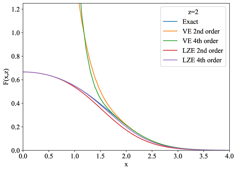
Figure 1: Comparison of VE [Eq. (45)] and LZE [Eq. (50)] representations of $F(x,z)$ in Eq. (44) at second and fourth orders, as a function of $x$ at $z=2$. The purple line showing the fourth-order LZE is barely distinguishable, on this scale, from the exact expression shown in blue.

IV Results

In this section we present our results, focusing on the universal thermodynamics of spin-$1/2$ fermions at unitarity. This is a system that is approximately realized in dilute neutron matter in the crust of neutron stars, and it is realized to great accuracy in ultracold atom experiments carried out by many groups around the world. Because of the wide interest in this problem from the condensed-matter, nuclear, and atomic physics communities, this system has been actively studied over the last two decades with progressively more accuracy, both theoretically as well as experimentally. Our purpose here is not to provide a more accurate answer for the thermodynamics but rather to use known results as a benchmark to assess the quality and range of validity of our method.

IV.1 Pressure at unitarity

As a first application of the QTCE, we show in Fig. 2 the pressure equation of state of spin-$1/2$ fermions at unitarity, compared with prior data from experiments as well as selected numerical approaches (including self-consistent diagrammatic [15] and Monte Carlo methods [16]). Specifically, we show in this plot the variation in our results when renormalizing using the second-order virial expansion (VE, shown in dashed gold line) or its fifth-order counterpart (solid gold line); the corresponding QTCE results are shown as light- and dark-shaded blue bands, respectively. The limits of the QTCE bands are set by renormalizing at $\beta\mu=-3.0$ and $\beta\mu=-1.0$; we find that the fifth-order VE renormalization scheme yields a much more constrained band than the second-order scheme. Remarkably, our results match the MIT [17] experimental results up to at least $\beta\mu=1.0$ (with a slight undershooting deviation around $\beta\mu=0$). We emphasize that the QTCE answer is given by a plain (no resummation) partial sum of the cumulant expansion of Eq. (12) up to $N_{\kappa}=6$ with the most rudimentary approximation for the imaginary-time direction, namely $N_{\tau}=1$.

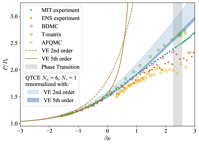
Figure 2: Pressure equation of state compared with other approaches. The VE is shown at second order with a dashed gold line and at fifth order [8] with a solid gold line. The experimental results from Ref. [17] are shown with green dots and those of Ref. [18] with red dots. The bold-diagrammatic Monte Carlo (BDMC) results of Ref. [19] appear as pink empty squares, the auxiliary-field quantum Monte Carlo (AFQMC) data of Ref. [16] is shown as orange empty squares, and the self-consistent results of Ref. [15] are given by the green empty squares. The vertical gray line around $\beta\mu=2.4$ shows the location of the superfluid phase transition bounded by values corresponding to a critical temperature of 0.152(7) [20] and 0.171(5) [21]. Finally, the QTCE results are shown as light- and dark-shaded blue bands, correspondingly marking the effects of renormalizing with the second- and fifth-order VE; the band limits are set by carrying out said renormalization at $\beta\mu=-3.0$ and $\beta\mu=-1.0$ in each case.

IV.2 Pressure in the BCS-BEC crossover

Extending our results beyond unitarity, in Fig. 2 we show the pressure as a function of $\beta\mu>0$, across the BCS-BEC crossover, for varying couplings parametrized by the ratio $\Delta b_{2}/\Delta b_{2}^{\text{UFG}}$ (shown with different colors). Here, $\Delta b_{2}$ is the interaction-induced change in the second-order virial coefficient, which is in one-to-one correspondence with the interaction strength as measured usually by the scattering length; $\Delta b_{2}^{\text{UFG}}=1/\sqrt{2}$ is the value in the unitary limit. In addition, the plot shows partial sums of the cumulant expansion up to order $N_{\kappa}$ (shown with different shades of the same color), indicating the highest power of $\lambda$ summed in the series of Eq. (12). All of the results shown in this plot correspond to $N_{\tau}=1$, i.e. the simplest possible Suzuki-Trotter factorization (i.e. the most coarse temporal lattice). For $\beta\mu<0$, there is no noticeable difference from varying $N_{\kappa}$, which means that the first cumulant, properly renormalized, is enough to capture the behavior of the curve.

The weakest coupling we considered is $\Delta b_{2}/\Delta b_{2}^{\text{UFG}}=0.01$, which is indistinguishable from the noninteracting limit in the scale shown in the plot. As the coupling is increased, the partial sums display oscillatory behavior at sufficiently large $\beta\mu$, indicating that the series must be resummed using methods such as Pade approximants. In particular, we note that the splitting of the partial sums coincides roughly (and not surprisingly) with the location of the superfluid phase transition (gray vertical band) around $\beta\mu=2.4$ in the unitary limit $\Delta b_{2}/\Delta b_{2}^{\text{UFG}}=1$ (blue lines).

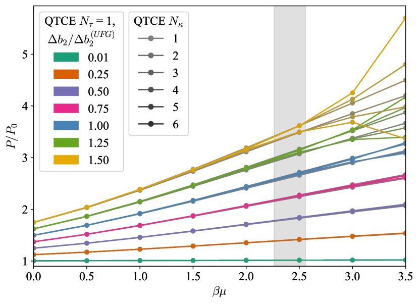
Figure 3: Pressure $P$, in units of the noninteracting pressure $P_{0}$, as a function of the coupling $\Delta b_{2}/\Delta b_{2}^{\text{UFG}}$ (shown in different colors), as obtained using the QTCE with $N_{\tau}=1$ and varying cumulant expansion order $N_{\kappa}$ (with the highest color saturation indicating $N_{\kappa}=6$).

IV.3 Beyond the pressure: density, compressibility and heat capacity at unitarity.

To characterize the thermodynamics of a system in a more detailed fashion, here we take a closer look at derivatives of the pressure, which yield the density equation of state and the elementary response functions given by the compressibility and heat capacity.

The density equation of state is accessed from Eq. (13) using the thermodynamic relation

$$N=\partialderivative{\ln{\mathcal{Z}}}{\ln z}=\partialderivative{\ln{\mathcal{Z}}}{(\beta\mu)}.$$ (53)

Taking further derivatives of the pressure, one may obtain the isothermal compressibility via the thermodynamic relation

$$\kappa_{T}=-\frac{1}{V}\left(\frac{\partial V}{\partial P}\right)_{T}=\frac{V\beta}{N^{2}}\partialderivative{N}{(\beta\mu)}$$ (54)

Our results for the density in the unitary limit are shown in Fig. 4. It is easy to see that, as for the pressure, the QTCE results, even at $N_{\tau}=1$, are a dramatic improvement over the fifth-order VE. As in Fig. 3, it is easy to see that as the superfluid phase transition is approached from low fugacity, the cumulant expansion displays wild oscillations that must be resummed.

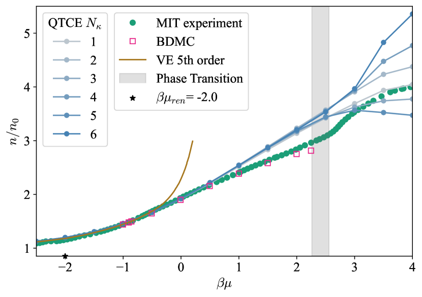
Figure 4: Density equation of state as a function of the dimension, for various chemical potentials. The $N_{\tau}=1$ QTCE results are shown in shades of blue according to the maximum cumulant order $N_{\kappa}$ included in the partial sums. The results of the MIT experiment of Ref. [17] are shown with green circles. The diagrammatic Monte Carlo results of Ref. [19] are shown with pink squares. The virial expansion results at fifth order are shown in gold [8].

Finally, the heat capacity per particle at unitarity is given by

$$\frac{C_{V}}{N}=\frac{1}{N}\left(\frac{\partial E}{\partial T}\right)_{N,V}=\frac{3}{5}\frac{d(P/P_{0,T=0})}{d(\beta E_{F})^{-1}},$$ (55)

where the first equality is the definition and the second equality is valid only at unitarity, where one may use the pressure-energy relation $E=3PV/2$; furthermore, we used $P_{0,T=0}={2nE_{F}}/{5}$, where $E_{F}=(3\pi^{2}n)^{2/3}/2$ is the Fermi energy of a noninteracting gas at density $n$.

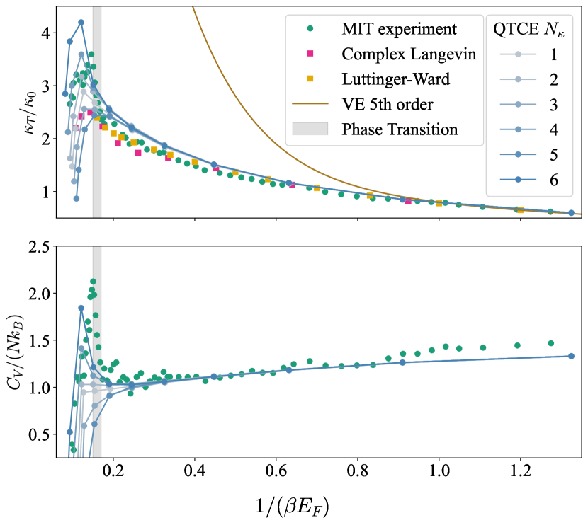
Figure 5: Top: Compressibility $\kappa_{T}$, in units of the ground-state noninteracting, zero temperature result $\kappa_{0}=3/(2nE_{F})$ as a function of the dimensionless temperature $T/E_{F}=1/(\beta E_{F})$. The green dots show the experimental results of Ref. [17], the pink squares show the complex Langevin results of Ref. [22], and the orange squares show the Luttinger-Ward results of Ref. [23]. The solid gold line indicates the result of the fifth-order virial expansion, using the results of Ref. [8]. Bottom: Heat capacity as a function of temperature. In both plots, the QTCE results are shown with full dots connected by straight lines, with shades of blue indicating the maximum order $N_{\kappa}$ summed in the cumulant expansion. The location of the superfluid phase transition is shown as a vertical gray band.

Our results for the compressibility and heat capacity are shown in Fig. 5. Both of these response functions show the correct qualitative features for temperatures above the superfluid transition. Moreover, the agreement with other approaches is arguably not merely qualitative. However, as with other quantities discussed above, dramatic oscillations appear in the cumulant expansion in low-temperature phase. This indicates that future analyses will require resummation approaches to interpret QTCE data when approaching a phase transition, which is not surprising.

IV.4 Continuous dimension at unitarity

One of the distinguishing aspects of QTCE is that it encodes the spatial dimension $d$ as an analytic variable that can be tuned continuously. To exemplify that capability, we show in Fig. 6 the results obtained for the pressure ratio $P/P_{0}$ as a function of $d$, for various chemical potentials, tuned to the unitary limit by renormalizing using the condition of matching at low fugacities with the fifth-order VE, as calculated in Ref. [8], across dimensions. We emphasize that we do not imply that this condition defines a unitary point in different dimensions; rather, it simply provides a way to formally renormalize the problem as $d$ is varied.

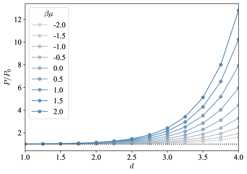
Figure 6: Pressure equation of state as a function of the dimension, for various chemical potentials, tuned to unitarity in 3D using the fifth-order VE.

As seen in Fig. 6, the interaction effects on $P$ disappear as $d$ is decreased. Put differently, weaker interactions are more easily able to reproduce the condition $\Delta b_{2}=1/\sqrt{2}$ in low dimensions than in high dimensions. In a real system, the physical picture behind this property is that a two-body bound state appears in 1D and 2D with vanishingly small attraction, which can dramatically increase $\Delta b_{2}$ already at weak coupling, as $\Delta b_{2}$ contains a term that increases exponentially with the binding energy.

The above observation suggests that, when renormalizing using the VE, one may expect the cumulant expansion (and more generally the QTCE results in coarse temporal lattices) to present better convergence properties in low dimensions. To explore that intuition, we show in Fig. 7 (top) the pressure as a function of $\beta\mu$ at unitarity, obtained with QTCE by dimensional extrapolation using data from $d=1.125$ to $d=2.5$, compared with QTCE exactly at $d=3.0$, as well as with the experimental results from MIT [17]. The results obtained with QTCE via extrapolation from low dimensions are clearly in much better quantitative agreement with the experimental numbers than those obtained by calculating directly in 3D.

In the bottom panel of Fig. 7, we provide a more detailed look at the dimension dependence of the pressure, at fixed $\beta\mu=2.5$, for $N_{\tau}=1$ and $N_{\kappa}=3$. There is a clear quantitative difference in the final results between taking the QTCE results at face value at $d=3$ (regardless of the resummation strategy or integrator used, as shown) and extrapolating from low dimensions (in this case between $d=1.125$ and $d=2.25$.

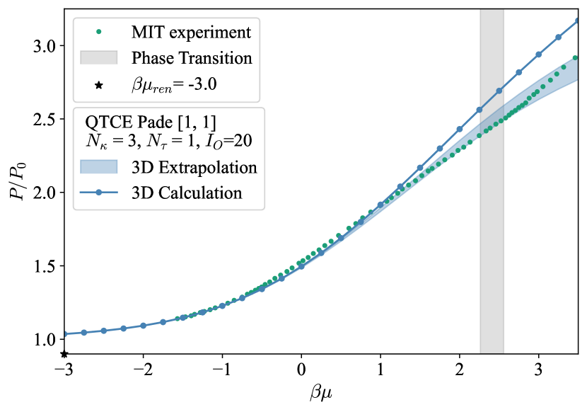
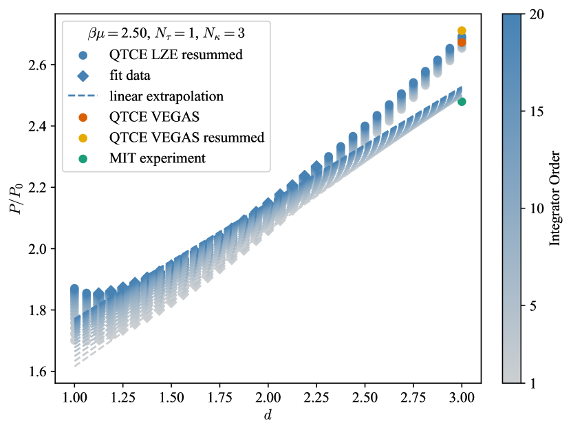
Figure 7: Top panel: Pressure equation of state as a function of $\beta\mu$ at unitarity. The green dots show the MIT data of Ref. [17]. The gray vertical region shows the superfluid phase transition. The star shows the value of $\beta\mu$ used to renormalize with the VE. The blue dots joined with a solid line show the results calculated in 3D and resummed using a Padé approximant. The shaded blue region shows the results calculated by dimensional extrapolation between $d=1.125$ and $d=2.0$ (bottom of band) to $d=2.5$ (top of band). Bottom panel: Spatial-dimension dependence of the pressure equation of state at $\beta\mu=2.5$. The shading from gray to blue indicates the results obtained using the LZE integrator at varying orders.

IV.5 Tests in lower dimensions

For completeness, we show in Fig. 8 a comparison of QTCE results at $N_{\tau}=1$ with a third-order perturbation theory calculation (in 1D; Ref. [24]) and auxiliary field quantum Monte Carlo calculations (in 2D; Ref. [25]) for the pressure as a function of $\beta\mu$. In 1D, the perturbation theory results are used to renormalize the QTCE calculation at $\beta\mu=-3.0$. In 2D, on the other hand, the second order virial expansion is used to renormalize at $\beta\mu=-3.0$. Also in both cases, it is clear that the results of QTCE at $N_{\tau}=1$ are superior to those of the virial expansion when increasing $\beta\mu$, even in the simplest possible case of $N_{\kappa}=1$. At sufficiently large $\beta\mu$, however, the partial sums of the QTCE cumulant expansion break down; in particular, they do so earlier in $\beta\mu$ for stronger couplings, as measured by the parameter $\lambda=2\sqrt{\beta}/a_{0}$ in 1D (unrelated to the QTCE parameter $\lambda$) and $\beta\epsilon_{B}$ in 2D, where $a_{0}$ is the 1D scattering length and $\epsilon_{B}$ is the binding energy of the two-body system.

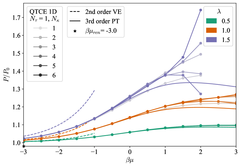
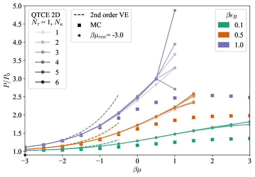
Figure 8: Top panel: pressure $P$ in units of the noninteracting pressure $P_{0}$, as a function of $\beta\mu$ for an attractively interacting 1D spin-$1/2$ Fermi gas. The solid lines with data points show the QTCE results; the purely solid lines show third-order perturbation theory, as obtained by Ref. [24]; and the dashed lines show the second order virial expansion. The different colors identify different couplings as parametrized by $\lambda$ and the different shades show varying orders in the QTCE cumulant expansion, as parametrized by $N_{\kappa}$. Finally, the star shows the renormalization point $\beta\mu=-3.0$ used by QTCE to calculate the coupling. Bottom panel: Same as top panel for the 2D Fermi gas. Instead of perturbation theory results, auxiliary field quantum Monte Carlo calculations are shown, as obtained by Ref. [25]. The coupling is parametrized by $\beta\epsilon_{B}$, where $\epsilon_{B}$ is the binding energy of the two-body problem.

V Beyond $N_{\tau}=1$ and integrator effects

In the previous sections we have shown results that reflect the successes and shortcomings of calculating in coarse temporal lattices. Naturally, it is desirable to remove such discretization effects altogether, e.g. by increasing $N_{\tau}$. For each diagram in our calculations, the cost of increasing $N_{\tau}$ is proportional to $N^{\alpha}_{\tau}$, where $\alpha$ is the number of loop integrals in the diagram. Thus, it becomes progressively more computationally expensive to increase $N_{\tau}$ when increasing $N_{\kappa}$. For those reasons, we only present here a discussion of $N_{\tau}$ effects that is very limited (specifically to $N_{\tau}<10$ ) compared with that of lattice Monte Carlo calculations which regularly operate at $N_{\tau}\sim 200$.

In Fig. 9, we show the effect of increasing $N_{\tau}$ on the assembled cumulants $\bar{K}_{n}$ (adding up all diagrammatic contributions up to order $N_{\kappa}=3$ at $d=3$). Note that the values presented here are coupling-independent: they reflect the diagrams’ structure induced by the theory and their dependence on $\beta\mu$.

As can be seen in the figure, the first row showing ${\bar{K}}_{1}$ displays no variation across integrators, simply because the required integrals are simple enough to be calculated by QTCE via Gaussian quadratures. In contrast, there is a clear variation in integrator approach when calculating ${\bar{K}}_{2}$ and ${\bar{K}}_{3}$: the stochastic result with VEGAS can differ substantially from the semi-analytical LZE result (shown at fixed integrator order $I_{0}=20$ in the right column and extrapolated to large integrator order in the middle column) at large enough $\beta\mu$. In all of these cases, however, the effects due to the imaginary-time discretization $N_{\tau}$ (shown with shades of different colors; see color key on the right side of the plot) are comparatively small: making $N_{\tau}=9$ (an extremely modest choice by conventional lattice Monte Carlo standards) yields an essentially converged result within a given integrator choice.

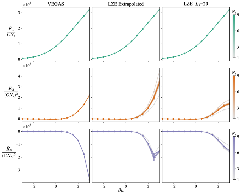
Figure 9: $N_{\tau}$ effects on the assembled cumulants in $d=3$, as a function of $\beta\mu$, for two different integrators: VEGAS (left column) and LZE at order 20 (right column). Note that we include $\bar{K}_{1}/N_{\tau}$ as a reference case that is actually $N_{\tau}$-independent and calculated exactly using Simpson integration methods. Note that $\bar{K}_{k}$ is proportional to $C^{k}$, which has also been factored out in order to obtain the coupling-independent quantities shown here.

Ultimately, the main lesson learned from studying these effects is that, remarkably, finite-temperature calculations can produce qualitatively (and in some non-trivial regions also quantitatively) correct results already at $N_{\tau}=1$.

VI Conclusion and Outlook

We have developed a semi-analytic approach to the nonrelativistic quantum many-body problem, which we call the QTCE. We have explored its capabilities by comparing with other theoretical approaches as well as experimental results in the unitary limit of the spin-$1/2$ Fermi gas.

We find that, with a renormalization scheme based on the VE, QTCE can capture the thermodynamics of the strongly coupled unitary gas in a remarkably natural way (meaning using mere partial sums and no resummation methods) with quantitative agreement with experiments in regions where the virial expansion fails. Moreover, this is accomplished without driving the number of imaginary time steps $N_{\tau}$ to a very high number: just a single time step captures the correct thermodynamics (pressure, density, compressibility, and heat capacity) up to $\beta\mu=1$ (which corresponds to temperatures down to $T/\epsilon_{F}$ = 0.3. On the other hand, QTCE at low $N_{\tau}$ does not capture the behavior at or beyond the superfluid phase transition ($\beta\mu\simeq 2.4$). Still, signatures of the transition do appear in QTCE results in the form of dramatic oscillations as the transition is approached from high temperatures.

Besides the above, we have probed the behavior of QTCE in 1D and 2D and as a continuous function of dimension (renormalizing to the 3D unitary point as a reference), where we also have full analytic control. This feature is interesting as studies of dimensional crossover become more common experimentally with ultracold atoms. From the theory standpoint, this is also a desirable feature, as the cumulant expansion may display better convergence properties at low or high dimensions, from where one may interpolate or extrapolate as needed.

The most straightforward generalizations of QTCE involve including higher spin degrees of freedom (in the form of higher number of species) or other quantum statistics (namely bosons). Beyond those, the generalization to polarized matter (with more than one fugacity variable) is also possible, as is the generalization to interactions beyond the density-density case, although the latter is more computationally intensive than the former. Both, however, would be relevant to tackle the problem of realistic neutron matter, especially if protons are to be included.