Unified Force and Motion Adaptive-Integral Control of
Flexible Robot Manipulators

Abstract

In this paper, an adaptive nonlinear strategy for the motion and force control of flexible manipulators is proposed. The approach provides robust motion control until contact is detected when force control is then available–without any control switch–, and vice versa. This self-tuning in mixed contact/non-contact scenarios is possible thanks to the unified formulation of force and motion control, including an integral transpose-based inverse kinematics and adaptive-update laws for the flexible manipulator link and contact stiffnesses. Global boundedness of all signals and asymptotic stability of force and position are guaranteed through Lyapunov analysis. The control strategy and its implementation has been validated using a low-cost basic microcontroller and a manipulator with 3 flexible joints and 4 actuators. Complete experimental results are provided in a realistic mixed contact scenario, demonstrating very-low computational demand with inexpensive force sensors.

1 Introduction

Increase interest on flexible manipulation has arisen mainly due to its potential for applications under weight constraints and physical interaction with the environment (possibly human). The resilience shown by these manipulators limits the negative effects of unforeseen impacts or other surrounding conditions, thus improving the stability and compliance under tasks involving physical interaction with the environment [13].

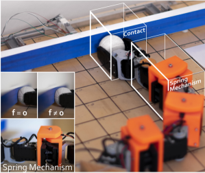
Figure 1: Lightweight flexible RM with force capabilities, highlighting the spring mechanism and the contact point.

Moreover, their flexible nature allows the implementation of force/impedance controllers [3, 7] and collision detection implementations [19], thus becoming a well-known solution for autonomous inspection [23] and assembly [15]. It is worth mentioning that their advantages in comparison with their rigid counterparts come at the cost of higher sensitivity to control delays, undesired flexible modes and less position accuracy (see e.g. high performance control of rigid-links manipulators in [22, 1]).

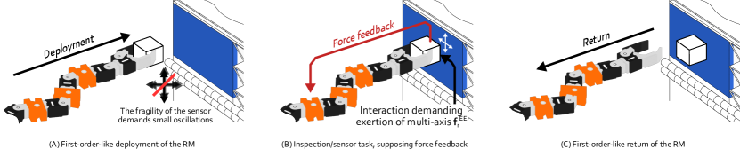
Figure 2: Phases of the complex task: inspection/installation of a sensor on an interface with multi-axis force demands.

To tackle these issues a two-pronged approach is essential: handling parameter uncertainty and rejecting external disturbances. This is generally pursued either by using i) adaptive techniques, including among others impedance/compliance control [20, 26], command-filtered backstepping [21], or neural networks [2]; ii) modified Inverse Kinematics (IK henceforth), varying from strategies taking into account the manipulator flexibility [27, 24], to variable impedance control [7]; or iii) sliding mode control [6, 16]. Nonetheless, these approaches tend to either compartmentalise the different control modes associated to separate phases of the complete task or depend on estimations with high sensitivity to model uncertainties. In fact, from our own experience, most of contact inspection tasks in non-structured environments are performed by breaking them down into simpler navigation and interaction sub-tasks (see sketch in Fig. 2) and awaiting for stabilisation in each one.

On the other hand, it is well known that the physical interaction changes the whole dynamics thus making manipulation fundamentally a nonlinear problem [12], often characterised through the mobility tensor. The proposed control strategy acts like an adaptive impedance interacting with the physical-environment admittance, fulfilling thus the complementarity of physical systems (input=rate and output=force), as shown in the seminal works [10, 11]. Moreover, its adaptive nature makes the controller perform well in both opposite extremes: rigid (low admittance) and soft (high admittance) environments. Thus, it is a non-trivial extension of the position-only controller of [4], where we had to increase its complexity to include force control which is strongly necessary for physical-interaction tasks. Here, the control objectives are the regulation of both position and force autonomously, unlike in there. By autonomously we mean that the controller itself decides how to adapt its impedance depending on the environmental admittance, to ensure asymptotic regulation to the prescribed references. The approach falls within the framework of closed-loop inverse kinematics, that fits perfectly with the physics of contact and combine position and force feedback thus guaranteeing good performance and stability. Additionally, it regulates the required force vector, not just in normal direction to the contact surface. Overall, the proposed controller for flexible robot manipulators is well suited for complex tasks such as contact inspection, sensor installation and polishing/cleaning.

The contributions are enumerated succinctly below:

• An impedance-like nonlinear adaptive control strategy capable of self-adjusting in mixed contact/non-contact scenarios, i.e. those with variable physical environment admittance. To the best of the authors’ knowledge, this is the first IK adaptive force and position smooth controller for flexible robot manipulators that works in unknown environments, rigid and soft.

• Force vector control at the contact point, decomposed in normal and tangential directions.

• Achieving C1 and C2 with a robust controller experimentally validated in a basic microcontroller, demonstrating very-low computational demand and, more importantly, with inexpensive force sensors (Fig. 1).

The paper is structured as follows: Section 2 outlines the background and framework; Section 3 is devoted to the controller design and main stability results; Section 4 to a thorough experimental validation; and finally, the paper is wrapped up with some conclusions.

Notation: All vectors are in bold, with $\mathbf{0}_{n}\in\mathbb{R}^{n}$ the zero vector. $0_{n\times m}\in\mathbb{R}^{n\times m}$ denote the zero matrix and $I_{n}$ the identity. For a matrix $A$, ${\rm ker}(A)$ denotes its kernel, ${\rm rank}(A)$ its rank and if $A>0$, $|\mathbf{v}|_{A}:=\mathbf{v}^{\top}A\mathbf{v}$ stands for the vector weighted norm. For a vector $\zeta$, $J_{\zeta}=\frac{\partial}{\partial\zeta}$ denotes the Jacobian and $J_{\zeta,\nu}$ the sub-block of $J_{\zeta}$ w.r.t the $\nu$-partition of $\zeta$; $\hat{\pi}$ reads as the $\pi$ estimate, and the operators column col$(\cdot)$ and block-diagonal matrix $\textnormal{diag}(\cdot)$. Acronyms: RM, Robot Manipulator; DoF, Degrees of Freedom; EE, End-Effector; and IK, Inverse Kinematics.

2 Background and framework

Let us consider a flexible robot manipulator whose joint-space configuration reads $\boldsymbol{\theta}:=\textnormal{col}(\boldsymbol{\gamma},\boldsymbol{\delta})$, where $\boldsymbol{\gamma}\in\mathbb{R}^{N}$ corresponds to the actuated angles and $\boldsymbol{\delta}\in\mathbb{R}^{M}$ to the flexible link deflections, as depicted in Fig. 3.

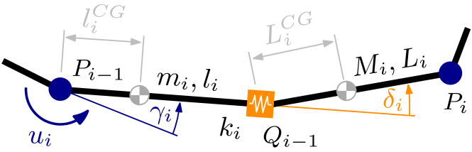
Figure 3: Definition of the DoF of the RM.

We then define its operational space as $\mathbf{q}:=\textnormal{col}({\mathbf{p}},{\boldsymbol{\alpha}})\in\mathbb{R}^{S}$, where ${\mathbf{p}}\in\mathbb{R}^{S_{p}}$ denotes the EE position and ${\boldsymbol{\alpha}}\in\mathbb{R}^{S_{\alpha}}$ its orientation, with $S=S_{p}+S_{\alpha}$. Thus, the manipulator kinematics reads

$$\dot{\mathbf{q}} =J\dot{\boldsymbol{\theta}}=J_{\gamma}\dot{\boldsymbol{\gamma}}+J_{\delta}\dot{\boldsymbol{\delta}},$$ (1a)

$$\dot{\mathbf{p}} =J_{p}\dot{\boldsymbol{\theta}}=J_{p,\gamma}\dot{\boldsymbol{\gamma}}+J_{p,{\delta}}\dot{\boldsymbol{\delta}},$$ (1b)

$$\dot{\boldsymbol{\alpha}} =J_{\alpha}\dot{\boldsymbol{\theta}}=J_{\alpha,\gamma}\dot{\boldsymbol{\gamma}}+J_{\alpha,{\delta}}\dot{\boldsymbol{\delta}}.$$ (1c)

Correspondingly, the joint-space dynamics of the flexible manipulator [5] for a EE contact force $\mathbf{f}\in\mathbb{R}^{S_{p}}$ becomes

$$B(\boldsymbol{\theta})\ddot{\boldsymbol{\theta}}+C(\boldsymbol{\theta},\dot{\boldsymbol{\theta}})\dot{\boldsymbol{\theta}}+\mathbf{k}(\boldsymbol{\delta})+\mathbf{g}(\boldsymbol{\theta})=\mathbf{u}-J_{p}^{\top}\mathbf{f},$$ (2)

where $B,C$ are the inertia and Coriolis terms matrices; $\mathbf{u}:=\textnormal{col}(\boldsymbol{\tau},\mathbf{0}_{M})$ includes the control torques $\boldsymbol{\tau}\in\mathbb{R}^{N}$, $\mathbf{g}:=\textnormal{col}(\mathbf{g}_{\gamma},\mathbf{g}_{\delta})$ the gravity, and $\mathbf{k}:=\textnormal{col}(\mathbf{0}_{N},K\boldsymbol{\delta})$ the flexible torques, with $K\in\mathbb{R}^{M\times M}$ the stiffness of the flexible links [25, 5].

2.1 Force and motion modeling

Let first define the task-space. In inverse kinematics, the task-space chosen $\mathbf{s}$ –also denoted as $\mathbf{q}$ in [8]–, is derived with respect to the actuated DoF and proven to converge to a reference using Lyapunov methods. We opt to include the contact forces in our task-space directly defined as $\mathbf{s}:=\textnormal{col}(\mathbf{q},\mathbf{f})$ and estimate its derivative as

$$\dot{\mathbf{s}}=\underbrace{\begin{pmatrix}J_{\gamma}\dot{\boldsymbol{\gamma}}+J_{\delta}\dot{\hat{\boldsymbol{\delta}}}\\ \dot{\hat{\mathbf{f}}}\end{pmatrix}}_{\mathrm{Estimate}}+\underbrace{\begin{pmatrix}J_{\delta}\dot{\tilde{\boldsymbol{\delta}}}\\ \dot{\tilde{\mathbf{f}}}\end{pmatrix}}_{\mathrm{Uncertain}}.$$

Intuitively, we need a model of $\boldsymbol{\delta},\mathbf{f}$ to capture the nature of $\dot{\boldsymbol{\delta}},\dot{\mathbf{f}}$. As the focus of this work is on contact, we choose the simple –but accurate– elastic contact model below. For, let first introduce the well-known elastic normal force model (without lateral force), as in [4], reading

$${\mathbf{f}}_{\top}={k}_{e}^{\top}\mathcal{N}^{\top}\left({\mathbf{p}}-{\mathbf{p}}_{s}\right),$$

with $\mathcal{N}^{\top}:=\mathbf{n}\mathbf{n}^{\top}$ the projection matrix on the outward contact normal $\mathbf{n}\in\mathbb{R}^{S_{p}}$, as in Fig. 4; $k_{e}^{\top}\in\mathbb{R^{+}}$ the unknown elastic modulus of the interface; and ${\mathbf{p}}_{s}\in\mathbb{R}^{S_{p}}$ the contact point at rest, i.e. without deformation. This formulation is enriched with elastic lateral forces where $\mathcal{N}^{\perp}:=I_{S_{p}}-\mathcal{N}^{\top}$ denotes the orthogonal projector matrix of $\mathcal{N}^{\top}$ and $k_{e}^{\perp}\in\mathbb{R^{+}}$ its unknown elastic parameter. Defining the elastic vector ${\mathbf{k}}_{e}:=\textnormal{col}({k}_{e}^{\top},{k}_{e}^{\perp})$ and using the matrix Kronecker product $\otimes$ the model reads

$${\mathbf{f}}=\big{(}{\mathbf{k}}_{e}^{\top}\otimes I_{S_{p}}\big{)}\left(\begin{array}[]{c}\mathcal{N}^{\top}\\ \mathcal{N}^{\perp}\end{array}\right)\left({\mathbf{p}}-{\mathbf{p}}_{s}\right)=:{K}_{e}\left({\mathbf{p}}-{\mathbf{p}}_{s}\right).$$ (3)

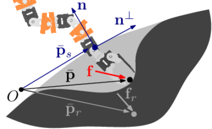
Figure 4: Definition of the contact parameters.

If we assume small flexible deflections, then their impact on the contact force is negligible and its derivative reads

$$\dot{{\mathbf{f}}}={K}_{e}J_{p,\gamma}\dot{\boldsymbol{\gamma}}.$$ (4)

Then, we proceed with the estimation of $\dot{\boldsymbol{\delta}}$. We opt for the inherently pseudo-static formulation in [27] coming from the components in $\boldsymbol{\delta}$ of (2), but including the proposed and complete force contact model in (3), namely

$$K{\boldsymbol{\delta}}=-J_{p,\delta}^{\top}{\mathbf{f}}+\mathbf{g}_{\delta},$$ (5)

where $\mathbf{g}_{\delta}:=J_{CG,\delta}^{\top}m\mathbf{g}_{0}$ –with $J_{CG,\delta}\in\mathbb{R}^{S_{p}\times M}$ linking the centre of mass of the manipulator and the flexible DoF–, $m$ is the mass of the RM, and $\mathbf{g}_{0}$ is the gravity acceleration in the inertial frame. Importantly, the factor structure of the proposed contact model (5) is instrumental to deal with the uncertainty of $\mathbf{k}_{e}$. Moreover, from (5) and using the properties of the Kronecker product an estimate of the flexible deflection rates becomes

$$\dot{{\boldsymbol{\delta}}}={K}^{-1}\Big{(}(\mathbf{k}_{e}^{\top}1)\otimes I_{M}\Big{)}J_{fg}\dot{\boldsymbol{\gamma}}=:-{\Theta}^{\top}J_{fg}\dot{\boldsymbol{\gamma}},$$ (6)

with the unknown matrix ${\Theta}\in\mathbb{R}^{3M\times M}$ and the compound force/gravity Jacobian $J_{fg}\in\mathbb{R}^{3M\times N}$ given by

$$J_{fg}{=}\begin{pmatrix}\big{(}I_{2}{\otimes}\dfrac{\partial J_{p,\delta}^{\top}}{\partial\boldsymbol{\gamma}}\big{)}\begin{pmatrix}\bar{N}^{\top}\\ \bar{N}^{\perp}\end{pmatrix}+\big{(}I_{2}{\otimes}J_{p,\delta}^{\top}\big{)}\begin{pmatrix}\mathcal{N}^{\top}\\ \mathcal{N}^{\perp}\end{pmatrix}J_{p,\gamma}\\ -\begin{pmatrix}\dfrac{\partial J_{CG,\delta}^{\top}}{\partial\gamma_{1}}&\cdots&\dfrac{\partial J_{CG,\delta}^{\top}}{\partial\gamma_{N}}\end{pmatrix}m\bar{G}\end{pmatrix},$$

with $\bar{N}^{\dagger}$, $\bar{G}\in\mathbb{R}^{NS_{p}\times N}$, $\scriptstyle\dagger:=\{\top,\perp\}$, defined column-wise as

$$\bar{\mathbf{N}}^{\dagger}_{k} :=\textnormal{col}_{k}\left(\mathbf{0}_{(k-1)S_{p}},(\mathcal{N}^{\dagger}({\mathbf{p}}-{\mathbf{p}}_{s})),\mathbf{0}_{(N-k)S_{p}}\right),$$

$$\bar{\mathbf{G}}_{k} :=\textnormal{col}_{k}\left(\mathbf{0}_{(k-1)S_{p}},\mathbf{g}_{0},\mathbf{0}_{(N-k)S_{p}}\right).$$

The model derived above allows to obtain the position and force uncertain error kinematics, where we use the estimates of the unknown elasticity matrices $K_{e}$ and $\Theta$ instead. Let the position and force errors be defined as $\mathbf{e}:=\mathbf{q}_{r}-\mathbf{q}\in\mathbb{R}^{S}$ and $\boldsymbol{\eta}:=\mathbf{f}_{r}-\mathbf{f}\in\mathbb{R}^{S_{p}}$, respectively, that are consistent with the task space. Then, using (1a), (4) and (6) the position and force error kinematics reads

$$\left.\begin{array}[]{r}\\ \mathrm{Position:}\\ \mathrm{Force:}\end{array}\right.\!\!\!\left.\begin{array}[]{c}\\ \dot{\mathbf{e}}=\\ \dot{\boldsymbol{\eta}}=\end{array}\right.\definecolor{tcbcolframe}{rgb}{1,0,0}\definecolor{tcbcolback}{rgb}{1,1,0.75}\definecolor{tcbcolback}{rgb}{0.85,0.85,1}\definecolor{tcbcol@origin}{rgb}{0,0,0}\definecolor{.}{rgb}{0,0,0}\definecolor{.}{rgb}{0,0,0}\leavevmode\hbox to60.33pt{\vbox to32.04pt{\text{[drawing]}}}\left.\begin{array}[]{c}\\ {+}\\ {-}\end{array}\right.\definecolor{tcbcolframe}{rgb}{1,0,0}\definecolor{tcbcolback}{rgb}{1,1,0.75}\definecolor{tcbcolback}{rgb}{1,0.85,0.85}\definecolor{tcbcol@origin}{rgb}{0,0,0}\definecolor{.}{rgb}{0,0,0}\definecolor{.}{rgb}{0,0,0}\leavevmode\hbox to64.33pt{\vbox to34.24pt{\text{[drawing]}}} \left.\begin{array}[]{c}\mathrm{Estimate}\\ \dot{\mathbf{q}}_{r}-\hat{J}_{T}(\hat{\Theta})\dot{\boldsymbol{\gamma}}\\ -\hat{K}_{e}J_{p,\gamma}\dot{\boldsymbol{\gamma}}\end{array}\right. \left.\begin{array}[]{c}\mathrm{Uncertain}\\ J_{\delta}\tilde{\Theta}^{\top}J_{fg}\dot{\boldsymbol{\gamma}}\\ \tilde{K}_{e}J_{p,\gamma}\dot{\boldsymbol{\gamma}}\end{array}\right. \left.\begin{array}[]{c}\mathrm{Estimate}\\ \dot{\mathbf{q}}_{r}-\hat{J}_{T}(\hat{\Theta})\dot{\boldsymbol{\gamma}}\\ -\hat{K}_{e}J_{p,\gamma}\dot{\boldsymbol{\gamma}}\end{array}\right. \left.\begin{array}[]{c}\mathrm{Uncertain}\\ J_{\delta}\tilde{\Theta}^{\top}J_{fg}\dot{\boldsymbol{\gamma}}\\ \tilde{K}_{e}J_{p,\gamma}\dot{\boldsymbol{\gamma}}\end{array}\right.$$ (7)

with $\hat{J}_{T}:=J_{\gamma}-J_{\delta}\hat{\Theta}^{\top}J_{fg}\in\mathbb{R}^{S\times N}$ the estimated Jacobian that includes the flexible behaviour from (6).

Remark 1.

In the position-only regulation strategy of [4] $\dot{\mathbf{q}}_{r}=\mathbf{0}$, whereas when including the force estimation in the control strategy the evolution of $\dot{\mathbf{q}}_{r}\neq\mathbf{0}$ is used during contact to achieve force regulation $\mathbf{f}=\mathbf{f}_{r}$, $\dot{\mathbf{f}}_{r}=0$.

3 Unified control strategy

The developed model (7) allows to define the adaptive integral IK and nonlinear force controller. For this non-trivial design, we start from the core position-regulation controller of [4] and augment it with the necessary structure. This includes an integral action $\boldsymbol{\xi}\in\mathbb{R}^{S}$ motivated from previous work with rigid manipulators of [22]. Its final intricate structure is depicted in Fig. 5 and reads

$$\dot{\boldsymbol{\xi}} =-K_{\xi}\boldsymbol{\xi}+K_{I}\hat{J}_{T}K_{\gamma}(\hat{J}_{T}^{\top}K_{P}\mathbf{e}+J_{p,\gamma}^{\top}\hat{K}_{e}\boldsymbol{\eta}),$$ (8a)

$$\dot{\boldsymbol{\gamma}} =K_{\gamma}\hat{J}_{T}^{\top}\left(K_{P}\mathbf{e}+K_{I}\boldsymbol{\xi}\right)+K_{\eta}J_{p,\gamma}^{\top}\hat{K}_{e}\boldsymbol{\eta},$$ (8b)

$$\dot{\mathbf{p}}_{r} =\hat{J}_{T}K_{\gamma\eta}J_{p,\gamma}^{\top}\hat{K}_{e}\boldsymbol{\eta}-\sigma(\left|\boldsymbol{\eta}\right|)K_{P}\mathbf{e},$$ (8c)

where the key scalar function $\sigma(\left|\boldsymbol{\eta}\right|)$, $\sigma(0)=0$, is positive definite; together with the adaptive update laws to cope with the uncertain contact model given by

$$\dot{\hat{\Theta}} =\Gamma_{\Theta}J_{fg}\dot{\boldsymbol{\gamma}}\hskip 0.85355pt\mathbf{e}^{\top}K_{P}J_{\delta},\quad\hat{\Theta}(0)=\Theta_{0},$$ (9a)

$$\dot{\hat{k}}_{e}^{\dagger} =\mathrm{Proj}({\varpi}_{\mathcal{N}^{\dagger}},\rho({\hat{k}}_{e}^{\dagger})),\quad\rho(\hat{k}_{e}^{\dagger}(0))\leq 1,$$ (9b)

where recall that we define the upper-index symbols $\scriptstyle\dagger=\{\top,\perp\}$ as the perpendicular projections of the force vector, and the projector operator $\mathrm{Proj}(\cdot,\cdot)$ [17, 14] associated to an suitable convex scalar function $\rho$; and

$${\varpi}_{\mathcal{N}^{\dagger}}(\boldsymbol{\xi},{\mathbf{e}},\boldsymbol{\eta}):= \ -\Gamma_{\mathcal{N}^{\dagger}}\ \boldsymbol{\eta}^{\top}{\mathcal{N}^{\dagger}}J_{p,\gamma}\dot{\boldsymbol{\gamma}},$$ (10)

being $K_{P},K_{I},K_{\xi},K_{\gamma},K_{\eta}$ and $\Gamma_{\Theta}$ positive definite matrices of appropriate dimensions, and $\Gamma_{\mathcal{N}^{\dagger}}\in\mathbb{R}^{+}$.

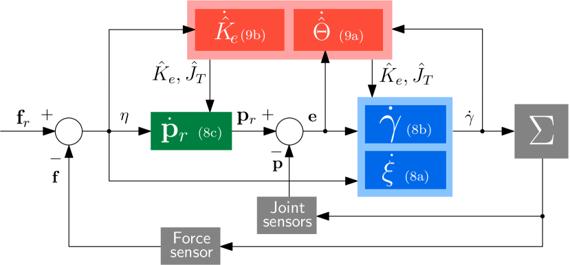
Figure 5: Control scheme: integral IK (blue, inner position loop); force-oriented change of references (green, outer force loop); and adaptive laws (orange). Equations in brackets.

Remark 2.

We underscore that the stiffness $K_{e}$ is completely unknown and the adaptation is in several force directions. Moreover, as it will be shown further, this controller is able to decide when to use the force and/or position depending on the actual physical interaction. Finally, even though the control architecture shows inner/outer-like position and force loops they are not in cascade but being strongly coupled with the adaptive update laws and the state interconnection through $(\ref{eq:control_pr})$ (see Fig. 5). Nonetheless, we show in the experiments that it can be implemented in a basic microcontroller.

3.1 Main stability result

Before stating the main stability result, let us rearrange the closed-loop kinematics plugging (8) in (7) and defining the state vector $\mathbf{x}:=\textnormal{col}(\boldsymbol{\xi},\mathbf{e},\boldsymbol{\eta})$. These result in

$$\dot{\mathbf{x}}=\hat{\mathcal{A}}(\mathbf{q},\hat{\Theta},\hat{K}_{e})\mathbf{x}+\tilde{\mathcal{B}}(\mathbf{q},\tilde{\Theta},\tilde{K}_{e})\dot{\boldsymbol{\gamma}},$$ (11)

with the estimation matrix $\hat{\mathcal{A}}$ defined as

$$\hat{\mathcal{A}} :=\left(\begin{array}[]{cc:c}-K_{\xi}&K_{I}\hat{\mathcal{J}}_{T}K_{P}&K_{I}\hat{\mathcal{J}}_{T\gamma}\hat{K}_{e}\\ -\hat{\mathcal{J}}_{T}K_{I}&-\big{(}\hat{\mathcal{J}}_{T}+\sigma(\left|\boldsymbol{\eta}\right|)I_{S}\big{)}K_{P}&\hat{\mathcal{J}}_{T\gamma}\hat{K}_{e}\\ \hdashline-\hat{K}_{e}\hat{\mathcal{J}}_{T\gamma}^{\top}K_{I}&-\hat{K}_{e}\hat{\mathcal{J}}_{T\gamma}^{\top}&-\hat{K}_{e}\mathcal{J}_{\gamma}\hat{K}_{e}\end{array}\right),$$

denoting $\hat{\mathcal{J}}_{T}:=\hat{J}_{T}K_{\gamma}\hat{J}_{T}^{\top}$, $\mathcal{J}_{\gamma}:=J_{p,\gamma}K_{\eta}J_{p,\gamma}^{\top}$, $\hat{\mathcal{J}}_{T\gamma}:=\hat{J}_{T}K_{\gamma}J_{p,\gamma}^{\top}$ and

$$\tilde{\mathcal{B}}:=\left(\begin{array}[]{cc:c}0_{N\times S}&J_{fg}^{\top}\tilde{\Theta}J_{\delta}^{\top}&-J_{p,\gamma}^{\top}\tilde{K}_{e}^{\top}\end{array}\right)^{\top}.$$

The next proposition states the main stability result.

Theorem 1 (Force control).

Consider the uncertain error system (7) and assume $\mathrm{rank}[J_{q}]=S$ and $\mathrm{rank}[J_{p,\gamma}]=S_{p}$ together with the design conditions $N\geq S$ and $N\geq S_{p}$. Define the function $\rho$ of $\mathrm{Proj}(\cdot,\rho)$ in (9b) convex and such that $|\hat{k}_{e}^{\dagger}(t)|>\epsilon$ for some constant $\epsilon>0$, $t\geq 0$; and $\sigma(\left|\boldsymbol{\eta}\right|)$, $\sigma(0)=0$ positive definite. Then, for any reference force $\mathbf{f}_{r}$ the adaptive-state feedback given by (8) and (9)-(10) guarantees global boundedness of all signals $\mathbf{x},\mathbf{p}_{r},{\hat{\Theta}}$ and $\hat{\mathbf{k}}_{e}$ and (globally) asymptotically stable zero equilibrium $\mathbf{x}=\mathbf{0}$.

Proof.

Let us define the radially unbounded and positive definite Lyapunov function candidate given by

$$V:=\dfrac{1}{2}\left|\mathbf{x}\right|^{2}_{\mathcal{K}}+\dfrac{1}{2}\mathrm{Tr}\left(\tilde{\Theta}^{\top}\Gamma_{\Theta}^{-1}\tilde{\Theta}\right)+\dfrac{1}{2}|{\tilde{\mathbf{k}}_{e}}|^{2}_{\Gamma^{-1}_{e}},$$ (12)

with $\mathcal{K}:=\textnormal{diag}(I_{S},K_{P},I_{S_{p}})$ and ${\Gamma_{e}}:=\textnormal{diag}(\Gamma_{k_{e}^{\top}},\Gamma_{k_{e}^{\perp}})$. Its derivative along the trajectories of (11) reads

$$\dot{V}=\mathbf{x}^{\top}\mathcal{K}\hat{\mathcal{A}}\mathbf{x}+\mathbf{x}^{\top}\mathcal{K}\tilde{\mathcal{B}}\dot{\boldsymbol{\gamma}}+\mathrm{Tr}\left(\tilde{\Theta}^{\top}\Gamma_{\Theta}^{-1}\dot{\tilde{\Theta}}\right)+{\tilde{\mathbf{k}}_{e}}^{\top}{\Gamma^{-1}_{e}}\dot{\tilde{\mathbf{k}}}_{e}.$$

This expression can be rewritten as

$$\dot{V}= -\boldsymbol{\xi}^{\top}K_{\xi}\boldsymbol{\xi}-\bar{\mathbf{e}}^{\top}(\hat{\mathcal{J}}_{T}+\sigma\left|\boldsymbol{\eta}\right|)\bar{\mathbf{e}}-\boldsymbol{\eta}^{\top}\hat{K}_{e}\mathcal{J}_{\gamma}\hat{K}_{e}\boldsymbol{\eta}$$

$$+\bar{\mathbf{e}}^{\top}J_{\delta}\tilde{\Theta}^{\top}J_{fg}\dot{\boldsymbol{\gamma}}-\mathrm{Tr}\left(\tilde{\Theta}^{\top}\Gamma_{\Theta}^{-1}\dot{\hat{\Theta}}\right)$$

$$-\boldsymbol{\eta}^{\top}\tilde{K}_{e}J_{\gamma}^{t}\dot{\boldsymbol{\gamma}}-{\tilde{\mathbf{k}}_{e}}^{\top}{\Gamma^{-1}_{e}}\dot{\hat{\mathbf{k}}}_{e}$$

$$= -\boldsymbol{\xi}^{\top}K_{\xi}\boldsymbol{\xi}-\bar{\mathbf{e}}^{\top}(\hat{\mathcal{J}}_{T}+\sigma\left|\boldsymbol{\eta}\right|)\bar{\mathbf{e}}-\boldsymbol{\eta}^{\top}\hat{K}_{e}\mathcal{J}_{\gamma}\hat{K}_{e}\boldsymbol{\eta}$$

$$+\mathrm{Tr}\left[\tilde{\Theta}^{\top}\left(-\Gamma_{\Theta}^{-1}\dot{\hat{\Theta}}+J_{fg}\dot{\boldsymbol{\gamma}}\bar{\mathbf{e}}^{\top}J_{\delta}\right)\right]$$

$$-{\tilde{\mathbf{k}}_{e}}^{\top}{\Gamma^{-1}_{e}}\left(\begin{array}[]{c}\mathrm{Proj}(\boldsymbol{\varpi}_{\mathcal{N}^{\top}},\rho({\hat{k}}_{e}^{\top}))-\boldsymbol{\varpi}_{\mathcal{N}^{\top}}\\ \mathrm{Proj}(\boldsymbol{\varpi}_{\mathcal{N}^{\perp}},\rho({\hat{k}}_{e}^{\perp}))-\boldsymbol{\varpi}_{\mathcal{N}^{\perp}}\end{array}\right)$$

where we have used $\bar{\mathbf{e}}:=K_{P}{\mathbf{e}}$ for compactness as well as the trace properties. By definition of the projector operator and the proposed update laws, we get

$$\dot{V}\leq-\boldsymbol{\xi}^{\top}K_{\xi}\boldsymbol{\xi}-\bar{\mathbf{e}}^{\top}(\hat{\mathcal{J}}_{T}+\sigma\left|\boldsymbol{\eta}\right|)\bar{\mathbf{e}}-\boldsymbol{\eta}^{\top}\hat{K}_{e}\mathcal{J}_{\gamma}\hat{K}_{e}\boldsymbol{\eta}.$$

Therefore, since $V>0$ globally and $\dot{V}\leq 0$, all the trajectories are bounded and the first claim follows.

For the stability claim and since the closed-loop is autonomous we analyse the largest invariant set included in the residual dynamics and invoke LaSalle’s Invariance Principle. Let first prove that the matrix $\hat{K}_{e}$ is invertible. By requirement the projectors ensure $\hat{k}_{e}^{\top},\hat{k}_{e}^{\perp}\neq 0$, then

$$\det(\hat{K}_{e}) =\det\left[\hat{k}_{e}^{\top}\mathbf{n}\mathbf{n}^{\top}+\hat{k}_{e}^{\perp}\left(I_{S_{p}}-\mathbf{n}\mathbf{n}^{\top}\right)\right]$$

$$=(\hat{k}_{e}^{\perp})^{S_{p}}\det\left[I_{S_{p}}+\left({\hat{k}_{e}^{\top}}/{\hat{k}_{e}^{\perp}}-1\right)\mathbf{n}\mathbf{n}^{\top}\right]$$

$$=(\hat{k}_{e}^{\perp})^{S_{p}-1}\hat{k}_{e}^{\top}\neq 0,$$

where the matrix determinant lemma has been invoked. From above we can define the vector $\hat{\boldsymbol{\eta}}:=\hat{K}_{e}\boldsymbol{\eta}$. Thus, the residual dynamics are defined in the set

$$\Omega:=\left\{\mathbf{x}\in\mathbb{R}^{2S+S_{p}};\hat{\Theta}\in\mathbb{R}^{3M\times M};\hat{\mathbf{k}}_{e}\in\mathbb{R}^{2}:\dot{V}=0\right\}.$$

We distinguish two cases $\boldsymbol{\eta}\neq\mathbf{0}$ and $\boldsymbol{\eta}=\mathbf{0}$, where it is straightforward to check, from (8) and (11), that the dynamics restricted to $\Omega$ become $\dot{\boldsymbol{\gamma}}=\dot{\mathbf{x}}=\dot{\hat{\Theta}}=\dot{\hat{\mathbf{k}}}_{e}=\mathbf{0}$, hence containing only fixed points and reducing the analysis to rule out all the undesirable equilibria.

[Case $\boldsymbol{\eta}\neq\mathbf{0}$]. Notice that, the function $\sigma$ is positive definite, and hence $\dot{V}=0\Leftrightarrow\boldsymbol{\xi}=\mathbf{e}=\mathbf{0}$ and $J_{p,\gamma}^{\top}\hat{\boldsymbol{\eta}}=\mathbf{0}$. The assumption $\mathrm{rank}(J_{p,\gamma})=S_{p}$ and the condition $N\geq S_{p}$ imply $\ker\big{[}J_{p,\gamma}^{\top}\big{]}=\mathbf{0}$ and therefore inducing injectivity that ensures $\hat{\boldsymbol{\eta}}=\mathbf{0}$.

[Case $\boldsymbol{\eta}=\mathbf{0}$]. In this case, by definition $\sigma_{p}=0$ and hence $\dot{V}=0\Leftrightarrow\boldsymbol{\xi}=\boldsymbol{\eta}=\mathbf{0}$ and $\hat{J}^{\top}_{T}\bar{\mathbf{e}}=\mathbf{0}$. Notice that $\hat{J}_{T}^{\top}=(\begin{array}[]{c:c}I_{N}&-J_{fg}^{\top}\hat{\Theta}\end{array})J_{q}^{\top}$ and let us define $v:=J_{q}^{\top}\bar{\mathbf{e}}\in\mathbb{R}^{N+M}$. By assumptions $\mathrm{rank}(J_{q})=S$ and $N\geq S$ thus inducing and injective map from $\bar{\mathbf{e}}$ to $v$. Hence, $\hat{J}^{\top}_{T}\bar{\mathbf{e}}=\mathbf{0}$ implies that $v\in\ker\left[(\begin{array}[]{c:c}I_{N}&-J_{fg}^{\top}\hat{\Theta}\end{array})\right]$ that is spanned by the columns of $J_{\hat{\Theta}}^{\perp}:=(\begin{array}[]{c:c}\hat{\Theta}^{\top}J_{fg}&I_{M}\end{array})^{\top}$ and then $v=J_{\hat{\Theta}}^{\perp}\varrho$ for some arbitrary $\varrho\in\mathbb{R}^{M}$. Consider now the linear map $v=J_{\hat{\Theta}}^{\perp}\varrho$ which has $\mathrm{rank}\big{[}J_{\hat{\Theta}}^{\perp}\big{]}=M$. Thus, $\ker\big{[}J_{\hat{\Theta}}^{\perp}\big{]}=\mathbf{0}$ which implies $J_{\hat{\Theta}}^{\perp}\varrho=\mathbf{0}\Leftrightarrow\varrho=\mathbf{0}$ and therefore $v=\mathbf{0}\Rightarrow\mathbf{e}=\mathbf{0}$. ∎∎

Corollary 1 (Unifying property).

Consider a non-contact case $\boldsymbol{\eta}\neq\mathbf{0}$ with a constant reference position $\mathbf{p}_{r}=\mathbf{p}_{r}^{*}$, with $\dot{\mathbf{p}}_{r}=0$ from (8c). Then, the adaptive-state feedback (8a)-(8b) and (9)-(10) guarantees (globally) asymptotically stable equilibrium $\mathbf{p}=\mathbf{p}_{r}^{*}$, $\dot{\boldsymbol{\eta}}=\mathbf{0}$.

Proof.

This result is a direct consequence from the case $\boldsymbol{\eta}\neq\mathbf{0}$ in the proof of Theorem 1. ∎∎

Remark 3.

Although straightforward from Theorem 1, Corollary 1 has been stated to highlight the unifying property. This means that the controller is able to follow alternate position and force demands without the need of changing its architecture, and hence being able to accomplish complex tasks as the one described in Fig. 2. To demosntrate this fact specifically, we propose a hybrid position-force scenario in the experimental validation.

4 Experimental validation results

To demonstrate the motion/force control capabilities, an experimental validation scenario is proposed: the tracking of a set of waypoints and multi-axis forces on a contact interface equipped with cheap force sensors shown in Fig. 6. The robot manipulator is composed of $N=4$ actuated DoF mounting Dynamixel AX-12A servomotors –with a resolution of 0.3$\mathrm{\SIUnitSymbolDegree}$ (0.0052 $\mathrm{rad}$), a stall torque of 1.5 $\mathrm{N}\text{\,}\mathrm{m}$ and lacking speed control mode – and $M=3$ flexible joints. The latter are designed with a low stiffness dual spring system –whose deflection is measured with Murata SV01 potentiometers–, being prone to nonlinear behaviours and, hence, highlighting the robustness of the control strategy. These two link typologies are placed alternatively, actuated followed by flexible (such as in Fig. 3), except for the last DoF that lacks the flexible one. All the parameters are shown in Table 1.

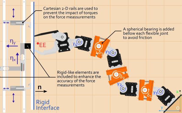
Figure 6: Experimental setting including rigid contact interface and force measurement system. Friction can be neglected due to the spherical bearings in the flexible joints.

Table 1: Benchmark application parameters

Compound joints [$\mathrm{cm}$, $\mathrm{g}$, $\mathrm{N}\text{\,}\mathrm{m}\text{\,}{\mathrm{rad}}^{-1}$]							EE joint [$\mathrm{cm}$, $\mathrm{g}$]
$l$	$L$	$l^{CG}$	$L^{CG}$	$m$	$M$	$k$	$l_{EE}$	$l^{CG}_{EE}$	$m_{EE}$
4.8	6.2	2.4	3.6	25	64	0.8	12.0	6.0	72

Table 2: Benchmark control gains

$K_{P}$		$K_{I}$		$K_{\xi}$		$K_{\gamma}$				$K_{\eta}$
$\bar{\mathbf{p}}$	$\bar{\boldsymbol{\alpha}}$	$\bar{\mathbf{p}}$	$\bar{\boldsymbol{\alpha}}$	$\bar{\mathbf{p}}$	$\bar{\boldsymbol{\alpha}}$	$1$	$2$	$3$	$4$	$1$	$2$	$3$	$4$
0.5949	0.0214	0.1610	0.0024	0.1200	0.1200	209.9	220.5	241.4	283.4	20.00	20.00	20.00	20.00
$\Gamma_{\Theta}$
$\Theta_{1}$	$\Theta_{2}$	$\Theta_{3}$	$\Theta_{4}$	$\Theta_{5}$	$\Theta_{6}$	$\sigma_{p}$	$\Gamma_{k_{e}^{\top}}$	$\Gamma_{k_{e}^{\perp}}$	$k_{M}^{\top}$	$k_{m}^{\top}$	$k_{M}^{\perp}$	$k_{m}^{\perp}$	$\beta$
257.1	1929	3857	51.43	385.7	771.4	0.3	0.0040	0.0020	0.0120	0.0040	0.0120	0.0040	0.4000

On the other hand, the dual-axis force sensor is formed by joining two linear bi-directional load cells in a $\Gamma$-shape as depicted in Fig. 6 and converting their signals using an HX711 ADC, thus obtaining relatively clean force measurement. Altogether, the system provides enough information to close the loop with acceptable accuracy.

To compute the feedback and the control algorithm, an Arduino Mega 2560, based on a 16 $\mathrm{MHz}$ ATmega2560 and with a flash memory of 256 $\mathrm{KiB}$ and an SRAM of 8 $\mathrm{KiB}$, is used. This controller board provides a stable frequency of 40 $\mathrm{Hz}$ throughout the experiment. We have chosen a planar RM for the validation just to simplify the force-measurement system and alleviate the computation load for this cheap microcontroller, but keeping the novelty of the vector force compensation. Finally, a projector operator consistent with Theorem 1 yields

$$\mathrm{Proj}({\varpi},\rho({\hat{\kappa}})):=\left\{\begin{array}[]{ll}\left[1-(\rho(\hat{\kappa})^{\prime})^{2}\right]\rho(\hat{\kappa})&{\varpi},\ \rho(\hat{\kappa})^{\prime}{\varpi}>0\\ {\varpi}&\mathrm{otherwise}\end{array}\right.,$$

being $\hat{\kappa}\in\mathbb{R}$ the parameter projected and $\rho$ the convex function which has been defined as

$$\rho({\hat{\kappa}}):=\dfrac{\left(\hat{\kappa}-\dfrac{\kappa_{M}+\kappa_{m}}{2}\right)^{2}}{\left(1-\beta^{2}\right)\left(\dfrac{\kappa_{M}-\kappa_{m}}{2}\right)^{2}}-\dfrac{\beta^{2}}{1-\beta^{2}}.$$

The positive definite function $\sigma$ is defined as $\sigma:=\sigma_{p}\left|\boldsymbol{\eta}\right|$, with constant $\sigma_{p}>0$ and the control gains and parameters used in all the experiments are shown in Table 2.

With the above experimental settings we propose two scenarios to validate the approach: i) an exclusively ad-hoc force control setting to validate the result of Theorem 1; and ii) a mixed scenario including unperturbed displacement and controlled contact forces, to validate the universal property combining the results of Theorem 1 and Corollary 1, hence providing an example of application with an implicit transition between the two modes. We underscore that these experiments also validate the computer implementation of the algorithm in a cheap microcontroller and the hardware control system.

4.1 Contact force scenario (force control)

\begin{overpic}[abs,unit=1mm,width=346.89731pt]{Exp2.pdf} \put(84.5,141.5){\rotatebox[origin={c}]{90.0}{\scalebox{0.5}{$\top$}}} \end{overpic}

Figure 7: Results of the contact force case: force tracking and adaptive contact parameters (top), with projector influence and contact detection; Cartesian position and orientation (centre, with modified references as lighter lines in contrast to the original ones, dotted); and $\hat{\Theta}$ parameters (bottom).

\begin{overpic}[abs,unit=1mm,width=424.94574pt]{Exp3.pdf} \put(101.2,79.1){\rotatebox[origin={c}]{90.0}{\scalebox{0.4}{$\top$}}} \end{overpic}

Figure 8: Results of the mixed contact/non-contact scenario, with: force regulation and adaptive contact parameters (top), including the projector influence zones; the Cartesian position and orientation (centre, with modified references as lighter lines and original ones dotted); and the whole set of adaptive parameters (bottom).

The force control—second phase in Fig. 2 B)–, is demonstrated for $\mathbf{f}_{r}=[-1,1.5]^{\top}$$\mathrm{N}$ and an initial condition close to the contact interface. As shown in Fig. 7, these force demands are achieved while the outer position loop derived from the modification of $\dot{\mathbf{p}}_{r}$ in (8c) converges to the trivial error. To obtain this outcome, nonetheless, some other parameters have a significant, but indirect, contribution. On the one hand, the adaptive contact parameters $\hat{k}_{e}^{\top},\hat{k}_{e}^{\perp}$ show slight variations that shape the rate of change of the position reference to obtain a safer response: decreasing its sensitivity to smooth the convergence when the forces are bellow their references and increasing it when these are excessive. On the other hand, the adaptive parameters $\hat{\Theta}$ are responsible of dampening the possible oscillations that could occur just after the first contact. Altogether, for a good validation the main contribution of Theorem 1 is demonstrated in this ad-hoc and clean scenario minimising other external factors, except noise and cheap computer implementation.

4.2 Mixed scenario (unified position and force control)

The second experiment, and the most interesting one showing the unified property, includes the interaction between the contact force and position reference changes. This scenario imitates the motivational task describen in the Fig. 2, where the controller has to follow a position-force-position references corresponding to the three phases. As it was shown in Corollary 1, the controller decides autonomously the ‘soft switching’ between them. These soft transitions are achieved without using any control switch or changing the control gains, just by the inherent cancellation of the outer loop when $\boldsymbol{\eta}=\mathbf{0}$. However, in practice the noise and the cheap force sensor hardware preclude the use of the equality condition and hence a threshold $\eta_{t}$ is introduced for its implementation as $\lvert\boldsymbol{\eta}\lvert<\eta_{t}\rightarrow\boldsymbol{\eta}=\mathbf{0}$, with constant $\eta_{t}>0$. The force reference is set as $\mathbf{f}_{r}=[0,2]^{\top}$$\mathrm{N}$, i.e. pressing without inducing tangential forces.

As thoroughly shown in Fig. 8, the interaction between these has no noticeable impact on the response, showing a first-order-like response when commanded to move before and after the contact. Additionally, it is worth going into the details of the indirect parameters, as done with the previous scenario. Firstly, the contact parameters show wider variations in this case (when they are not cancelled by $\lvert\boldsymbol{\eta}\lvert<\eta_{t}$ before and after contact), not having any significant impact on the force tracking convergence apart from the mere experimental variability. Secondly, the results of the matrix of adaptive parameters associated with the flexibility of the RM are completely consistent with the previous scenario. However, two comments ought to be included: i) the aforementioned difference in their order of magnitude between contact and displacement make their variation in the former case indistinguishable; and ii) the terms associated to $\mathcal{N}^{\perp}$ in $\hat{\Theta}$ are quite noticeable after contact, the only difference with respect to the previous scenario.

5 Conclusions

An adaptive force and motion control strategy for flexible manipulators is presented. Thanks to its adaptive nature, this controller is well-suited for the installation of fragile devices demanding controlled force. While its multi-axis force capabilities allow performing contact tasks converging to these force demands, the adaptation to the stiffness of the flexible links provides disturbance rejection capabilities, that increase the accuracy of the operation and reduce the risk of incidents. Together with a detailed derivation using well-known Lyapunov-based control techniques, full theoretical and experimental results are provided. Among the latter, it is worth highlighting the scenario including both abrupt position reference changes and force regulation, thus demonstrating the suitability of the control strategy for applications with mixed contact/non-contact scenarios that provide variable environmental admittance.

References

• Acosta et al. [2020] Acosta, J.A., de Cos, C.R., Ollero, A., 2020. Accurate control of aerial manipulators outdoors. a reliable and self-coordinated nonlinear approach. Aerospace Science and Technology 99, 105731. URL: http://www.sciencedirect.com/science/article/pii/S1270963819305176, doi:https://doi.org/10.1016/j.ast.2020.105731.
• Cheng et al. [2009] Cheng, L., Hou, Z.G., Tan, M., 2009. Adaptive neural network tracking control for manipulators with uncertain kinematics, dynamics and actuator model. Automatica 45, 2312–2318. URL: https://www.sciencedirect.com/science/article/pii/S0005109809002982, doi:https://doi.org/10.1016/j.automatica.2009.06.007.
• Colomé et al. [2013] Colomé, A., Pardo, D., Alenyà, G., Torras, C., 2013. External force estimation during compliant robot manipulation, in: 2013 IEEE International Conference on Robotics and Automation (ICRA), pp. 3535–3540. doi:10.1109/ICRA.2013.6631072.
• de Cos et al. [2020] de Cos, C.R., Acosta, J.A., Ollero, A., 2020. Adaptive integral inverse kinematics control for lightweight compliant manipulators. IEEE Robotics and Automation Letters 5, 282–289.
• De Luca and Book [2016] De Luca, A., Book, W.J., 2016. Robots with flexible elements, in: Springer Handbook of Robotics. Springer, pp. 243–282.
• El Makrini et al. [2016] El Makrini, I., Rodriguez-Guerrero, C., Lefeber, D., Vanderborght, B., 2016. The variable boundary layer sliding mode control: A safe and performant control for compliant joint manipulators. IEEE Robotics and Automation Letters 2, 187–192.
• Ficuciello et al. [2015] Ficuciello, F., Villani, L., Siciliano, B., 2015. Variable impedance control of redundant manipulators for intuitive human–robot physical interaction. IEEE Transactions on Robotics 31, 850–863. doi:10.1109/TRO.2015.2430053.
• Galicki [2016] Galicki, M., 2016. Finite-time trajectory tracking control in a task space of robotic manipulators. Automatica 67, 165–170. URL: https://www.sciencedirect.com/science/article/pii/S0005109816000261, doi:https://doi.org/10.1016/j.automatica.2016.01.025.
• Heck et al. [2016] Heck, D., Saccon, A., van de Wouw, N., Nijmeijer, H., 2016. Guaranteeing stable tracking of hybrid position–force trajectories for a robot manipulator interacting with a stiff environment. Automatica 63, 235–247. URL: https://www.sciencedirect.com/science/article/pii/S000510981500429X, doi:https://doi.org/10.1016/j.automatica.2015.10.029.
• Hogan [1984] Hogan, N., 1984. Impedance control: An approach to manipulation, in: 1984 American control conference, IEEE. pp. 304–313.
• Hogan [1985] Hogan, N., 1985. Impedance Control: An Approach to Manipulation: Part I—Theory. Journal of Dynamic Systems, Measurement, and Control 107, 1–7. URL: https://doi.org/10.1115/1.3140702, doi:10.1115/1.3140702.
• Hogan [1987] Hogan, N., 1987. Stable execution of contact tasks using impedance control, in: Proceedings. 1987 IEEE International Conference on Robotics and Automation, IEEE. pp. 1047–1054.
• Hogan [2022] Hogan, N., 2022. Contact and physical interaction. Annual Review of Control, Robotics, and Autonomous Systems 5, 179–203. URL: https://doi.org/10.1146/annurev-control-042920-010933, doi:10.1146/annurev-control-042920-010933, arXiv:https://doi.org/10.1146/annurev-control-042920-010933.
• Ioannou and Sun [1995] Ioannou, P.A., Sun, J., 1995. Robust Adaptive Control. Prentice-Hall, Inc., USA.
• Jimenez-Cano et al. [2013] Jimenez-Cano, A.E., Martin, J., Heredia, G., Ollero, A., Cano, R., 2013. Control of an aerial robot with multi-link arm for assembly tasks, in: 2013 IEEE International Conference on Robotics and Automation, pp. 4916–4921. doi:10.1109/ICRA.2013.6631279.
• Kashiri et al. [2014] Kashiri, N., Tsagarakis, N.G., Van Damme, M., Vanderborght, B., Caldwell, D.G., 2014. Enhanced physical interaction performance for compliant joint manipulators using proxy-based sliding mode control, in: 2014 11th International Conference on Informatics in Control, Automation and Robotics (ICINCO), IEEE. pp. 175–183.
• Krstic et al. [1995] Krstic, M., Kokotovic, P.V., Kanellakopoulos, I., 1995. Nonlinear and Adaptive Control Design. 1st ed., John Wiley & Sons, Inc., USA.
• Li et al. [2008] Li, Z., Ge, S., Adams, M., Wijesoma, W., 2008. Robust adaptive control of uncertain force/motion constrained nonholonomic mobile manipulators. Automatica 44, 776–784. URL: https://www.sciencedirect.com/science/article/pii/S0005109807003627, doi:https://doi.org/10.1016/j.automatica.2007.07.012.
• Luca et al. [2006] Luca, A.D., Albu-Schaffer, A., Haddadin, S., Hirzinger, G., 2006. Collision detection and safe reaction with the DLR-III lightweight manipulator arm, in: 2006 IEEE/RSJ International Conference on Intelligent Robots and Systems (IROS), pp. 1623–1630. doi:10.1109/IROS.2006.282053.
• Luo et al. [2013] Luo, R.C., Y.W. Perng, B.H. Shih, Y.H. Tsai, 2013. Cartesian position and force control with adaptive impedance/compliance capabilities for a humanoid robot arm, in: 2013 IEEE International Conference on Robotics and Automation (ICRA), pp. 496–501. doi:10.1109/ICRA.2013.6630620.
• Pan et al. [2018] Pan, Y., Wang, H., Li, X., Yu, H., 2018. Adaptive command-filtered backstepping control of robot arms with compliant actuators. IEEE Transactions on Control Systems Technology 26, 1149–1156. doi:10.1109/TCST.2017.2695600.
• Sánchez et al. [2015] Sánchez, M.I., Acosta, J., Ollero, A., 2015. Integral action in first-order closed-loop inverse kinematics. application to aerial manipulators, in: Robotics and Automation (ICRA), 2015 IEEE International Conference on, pp. 5297–5302.
• Sanchez-Cuevas et al. [2020] Sanchez-Cuevas, P.J., Gonzalez-Morgado, A., Cortes, N., Gayango, D.B., Jimenez-Cano, A.E., Ollero, A., Heredia, G., 2020. Fully-actuated aerial manipulator for infrastructure contact inspection: Design, modeling, localization, and control. Sensors 20, 4708.
• Siciliano [2000] Siciliano, B., 2000. Parallel force and position control of flexible manipulators. Control Theory and Applications, IEEE URL: http://ieeexplore.ieee.org/xpls/abs{_}all.jsp?arnumber=903453.
• Siciliano et al. [2009] Siciliano, B., Sciavicco, L., Villani, L., Oriolo, G., 2009. Robotics. Modelling, planning and control. Springer-Verlag (UK).
• Siciliano and Villani [1996] Siciliano, B., Villani, L., 1996. Adaptive compliant control of robot manipulators. Control Engineering Practice 4, 705 – 712. URL: http://www.sciencedirect.com/science/article/pii/0967066196000548, doi:https://doi.org/10.1016/0967-0661(96)00054-8.
• Siciliano and Villani [2001] Siciliano, B., Villani, L., 2001. An inverse kinematics algorithm for interaction control of a flexible arm with a compliant surface. Control Engineering Practice 9, 191–198. doi:10.1016/S0967-0661(00)00097-6.