Applying Machine Learning Techniques to Searches for Lepton-Partner
Pair-Production with Intermediate Mass Gaps at the Large Hadron Collider

Abstract

We consider the application of machine learning techniques to searches at the Large Hadron Collider (LHC) for pair-produced lepton partners which decay to leptons and invisible particles. This scenario can arise in the Minimal Supersymmetric Standard Model (MSSM), but can be realized in many other extensions of the Standard Model (SM). We focus on the case of intermediate mass splitting ($\sim 30\,{\rm GeV}$) between the dark matter (DM) and the scalar. For these mass splittings, the LHC has made little improvement over LEP due to large electroweak backgrounds. We find that the use of machine learning techniques can push the LHC well past discovery sensitivity for a benchmark model with a lepton partner mass of $\sim 110\,{\rm GeV}$, for an integrated luminosity of $300~{}\rm fb^{-1}$, with a signal-to-background ratio of $\sim 0.3$. The LHC could exclude models with a lepton partner mass as large as $\sim 160\,{\rm GeV}$ with the same luminosity. The use of machine learning techniques in searches for scalar lepton partners at the LHC could thus definitively probe the parameter space of the MSSM in which scalar muon mediated interactions between SM muons and Majorana singlet DM can both deplete the relic density through dark matter annihilation and satisfy the recently measured anomalous magnetic moment of the muon. We identify several machine learning techniques which can be useful in other LHC searches involving large and complex backgrounds.

I Introduction

A wide variety of scenarios for physics beyond the Standard Model (BSM) have been probed experimentally with the Large Hadron Collider (LHC). However, as no conclusive evidence of BSM physics has been found yet, focus has turned to scenarios and signatures which are more difficult to probe. One particularly difficult scenario is the pair production of scalar lepton partners of SM fermions ($\tilde{\ell}^{\pm})$, each of which decays to a lepton and an invisible particle ($\tilde{\ell}\rightarrow\ell X$) with a $\sim 30\,{\rm GeV}$ mass splitting. This scenario can arise in the minimal supersymmetric standard model (MSSM), as well as in other BSM models often specifically motivated by the need for a viable dark matter candidate and by recent measurements of the anomalous magnetic moment of the muon. This scenario is difficult to probe at the LHC because there is a large SM background from the production of electroweak gauge bosons, decaying to leptons and neutrinos. As a result, current LHC constraints [1] on this scenario show little improvement over LEP [2]. Although a variety of new analysis strategies have been proposed, there is no clear-cut strategy for effectively separating signal from background in models with these moderately compressed particle spectra. In this work, we investigate the possibility of using machine learning algorithms to more effectively pick out signal from background.

The standard signature of scalar lepton partner pair production at the LHC is $\bar{\ell}\ell$ plus missing transverse energy ${/\!\!\!\!E}_{\rm T}$ (MET). However, if the mass splitting is $\lesssim 60~{}\,{\rm GeV}$, then the lepton and invisible particles are both soft, and it is difficult to see this signature above the electroweak background. One strategy used to evade the difficulty of soft particles is to search for events in which one or more hard jets are also emitted ($pp\rightarrow\tilde{\ell}^{*}\tilde{\ell}+~{}{\rm jets}$). This jet provides a transverse kick to the $\tilde{\ell}^{*}\tilde{\ell}$ system, yielding harder leptons and larger MET. Even so, distinguishing signal events from the large electroweak background requires additional techniques. If the mass splitting is small ($\lesssim 20~{}\,{\rm GeV}$), then the electroweak background can be rejected because the neutrinos produced by $W$ decay typically carry larger MET than carried by the $X$ arising from $\tilde{\ell}$ decay. The efficacy of this search strategy has been enhanced by recent experimental developments, resulting in lower energy thresholds for lepton identification. However, searches at the LHC are still challenging for intermediate mass splittings in the range of $\sim 20-50~{}\,{\rm GeV}$.

Theoretical work has shown that progress can be made for mass splittings in the $\sim 20-50~{}\,{\rm GeV}$ range, using a variety of kinematic variables involving the energies of the leptons and jets and MET, as well as their angular correlations with each other [3]. But the progress is incremental; even applying these strategies, a model with $m_{\tilde{\ell}}=160~{}\,{\rm GeV}$ and $m_{\tilde{\ell}}-m_{X}=30~{}\,{\rm GeV}$ would be well out of reach of LHC with $300~{}\rm fb^{-1}$ luminosity. Moreover, there is no clean set of simple cuts which one can apply to maximize sensitivity, based on an a priori principle. Instead, one sequentially applies cuts to many kinematic variables, with each cut (and the order of cuts) being determined largely by trial and error. This is the type of setting in which one might expect machine learning algorithms to greatly improve search sensitivity, by determining the optimal set of cuts to impose on a large number of kinematic variables which can exhibit strong (nonlinear) correlations. Additionally, one might hope that it would be possible to work backwards after an optimal set of cuts is found to determine the underlying principle(s) responsible for the efficacy of those cuts. We will see that both of these intuitions are true.

In this work, we consider a benchmark point which is allowed by current constraints where the scalar lepton is a partner to the left-handed muon, with $m_{\tilde{\ell}}=110~{}\,{\rm GeV}$, $m_{\tilde{\ell}}-m_{\chi}=30~{}\,{\rm GeV}$. We use a boosted decision tree (BDT) to classify events as signal or background, finding that a cut based on the BDT classifier can increase the LHC sensitivity to $\gtrsim 5\sigma$ while maintaining a signal-to-background ratio of $\sim 0.3$ with $300~{}\rm fb^{-1}$ of data. We identify kinematic variables that dominantly contribute to the signal sensitivity and plot the residual distribution as applicable.

Importantly, we find that direct application of a BDT algorithm to simulated data is not sufficient. Essentially, because some SM background processes have very large rates, application of a BDT algorithm to an uncurated data sample will succeed at removing the largest backgrounds, while leaving subleading backgrounds which limit sensitivity. Instead, we adopt a strategy in which some initial precuts are imposed to reduce leading backgrounds with easily identified characteristics, leaving the BDT free to focus subsequently on more challenging features of the residual leading and subdominant backgrounds.

In a similar vein, we find that generation of the training sample used by the BDT also requires special care, because the most difficult backgrounds to remove lie in regions of phase space with relatively small cross section (though larger than the signal). If these regions of phase space are not adequately sampled by simulation, then the BDT can become overly focused on the details of a few particular events in the training sample. To avoid this problem, we generate simulation in kinematic tranches, significantly enhancing the fraction of computational time devoted to kinematic regions having smaller cross sections but larger pass rates for standard cuts.

In previous studies, a variety of machine learning techniques have been proposed and implemented for analyses of LHC data in which the BSM signal is particularly challenging to differentiate from the SM background. Following an early proposal for the use of BDTs and neural networks (NNs) in the analysis of pair production of fermionic partners of SM electroweak gauge bosons [4], this signal model (which is similar to scalar lepton production) has been constrained at LHC [1] using a BDT. For boosted topologies, both BDT and NN analyses have been shown to enhance the sensitivity of LHC searches to dark matter models with extended Higgs sectors [5]. Analyses of monojet plus missing energy signatures at LHC in several simplified dark matter models with mediators of different spins has demonstrated that NNs are able to efficiently determine if there is a BSM signal within a given dataset when trained on two-dimensional histograms combining information from different kinematic variables [6, 7].

In addition to supervised learning applications, less supervised techniques have been proposed for BSM searches at LHC. Weakly supervised techniques have been shown to increase the sensitivity of monojet plus missing energy searches to strongly interacting dark matter models with anomalous jet dynamics [8] and self-supervised contrastive learning has been proposed for anomaly detection searches in dijet events [9]. Complementing these largely model-agnostic techniques, adversarial NNs have also been suggested as an unsupervised approach to improve the invariant mass reconstruction of BSM gauge bosons decaying to leptons and neutrinos [10].

In this work, we favor an application of supervised learning strategies using a BDT due to the relatively straightforward manner in which the algorithm classifies signal and background events, facilitating a clear interpretation of results. We will focus not only on the search sensitivity which is achieved by application of a BDT, but also on what the BDT teaches us regarding the underlying search strategy, and on improved techniques for applying machine learning to general LHC searches with large and complex backgrounds.

The search strategy we propose is relevant for a variety of phenomenologically motivated extensions of the SM. For example, charged mediator models with a Majorana SM-singlet dark matter candidate and scalar muon partners mediating interactions with the SM can both satisfy the dark matter relic density and account for the anomalous magnetic moment of the muon [11]. With the coupling of the dark matter to the muon and its scalar partner fixed by the SM hypercharge coupling, as in the MSSM, the relic density in such models can be depleted by scalar mediated dark matter annihilation for lepton partner masses $m_{\tilde{\ell}}\lower 3.01385pt\hbox{$\;\stackrel{{\scriptstyle\textstyle<}}{{\sim}}\;$}150~{}\,{\rm GeV}$ [12] and by co-annihilation processes involving the scalars for $m_{\tilde{\ell}}\lower 3.01385pt\hbox{$\;\stackrel{{\scriptstyle\textstyle<}}{{\sim}}\;$}1~{}\,{\rm TeV}$ [13]. For simplified models with dark matter-scalar-lepton couplings larger than in the MSSM, both production mechanisms can yield the observed dark matter relic density for scalar masses $m_{\tilde{\ell}}\lower 3.01385pt\hbox{$\;\stackrel{{\scriptstyle\textstyle>}}{{\sim}}\;$}1~{}\,{\rm TeV}$ [13, 14]. Charged mediator models with the most massive scalar muon partners mentioned above are virtually impossible to detect at LHC due to the falling production cross sections at higher scalar masses. However, there are large regions of unconstrained parameter space which are challenging but feasible to probe for LHC searches with the improved sensitivity of analyses using machine learning techniques such as a BDT.

The plan of this paper is as follows. In Section II, we describe our approach and motivation for using a BDT. We outline the scalar muon partner signal and associated backgrounds, along with a summary of previously implemented and proposed analyses using cut-and-count strategies, in Section III. The details of the event simulation, selected observables, BDT training, and results of our analysis are described in Section IV. We discuss the conventional wisdom which can be gained from our study and applied to others in Section V, before summarizing our findings and briefly discussing future work in Section VI.

II Background and Motivation for Using a BDT

By its nature, known physics is necessarily more prevalent or more readily visible to conventional experimental techniques than unknown physics, while unknown physics and the opportunity to extend our understanding of fundamental particles and interactions are of greater basic interest. Accordingly, the problem of how one efficiently suppresses known backgrounds in order to enhance the prospective visibility of new processes is of great interest. In a prior study [3], we attempted to systematically separate the signal associated with the production of lepton-partners in intermediate mass gap scenarios from competing SM backgrounds via an iterative process involving the plotting of distributions in relevant kinematic observables and the manual application of event selection cuts. This approach proved effective, although there are a number of ways in which it is potentially sub-optimal.

Firstly, it was observed that this process is extremely sensitive to the order in which the cuts are applied, since a variety of useful secondary and tertiary event selections remain obscured until a majority of foreground debris is removed by primary selections. A corollary of this statement is that the possible sequencing of cuts explodes combinatorically, and it is very difficult to be certain that a given sequence of cuts is in any sense optimal. Likewise, there is a great danger that early event selections can be applied too aggressively, precluding more surgically targeted cuts down the line. This is part of a larger problem, that any by-hand procedure is intrinsically ad hoc and one-off, while simultaneously remaining extremely labor-intensive. Finally, there is a risk of biasing the analysis in the limit of low statistics, which always ultimately applies as selections become increasingly strict, since cuts are typically engineered and validated with respect to the same collection of events.

Machine learning offers substantial promise for alleviating negative outcomes associated with each of these objections. Specifically, it can much more thoroughly and efficiently scan the space of available discriminants, while delivering results that are more stable and more reproducible, using a generalizable approach that has increased cross-applicability, and which requires less investment of human capital into repetitive and automatable tasks. Additionally, leading machine learning algorithms offer built-in protection against over fitting. For example, the learning rate can be turned down such that the likelihood of over-applying an early selection and losing sensitivity to future gains is reduced. Likewise, the training and testing samples can be readily isolated, reducing the risk of learning random features of the presented sample that are not replicated in the larger ensemble. Also, the separation between training and testing can typically be “folded” in multiple ways, allowing for cross-validation via replication of the analysis, which helps to quantify the stability of results against statistical fluctuations. Much greater complexity and refinement of the discriminant is available in a machine learning context relative to manual approaches. Additionally, the assignment of a continuous event-by-event classification likelihood represents a much richer category of information than the discretization implicit to a more basic cut-and-count approach.

However, a pressing concern associated with machine learning is that one often sacrifices the ability to investigate what was learned, and to develop intuition regarding the nature of the signal and background separation. This is a key reason that we favor the use of supervised learning with a boosted decision tree over more sophisticated types of deep learning such as neural networks. In particular, the input to a boosted decision tree is a simple list of numerical data associated with each event, together with an event weight and a known classification in the case of the training sample. The BDT goes through a process that is similar to the design of a manual event selection profile in many regards, but it is strictly systematic, mathematically rigorous, and reproducible. At each stage of training, the optimal discriminant and splitting value is ascertained according to a well-defined loss function; subsequently, each branch of this “tree” can elect its own best choice for the next splitting, and so on. Likewise, the classification score assigned to each terminal leaf of the tree is selected by extremization of the same functional, in the effort to optimally reconcile feature-based predictions with corresponding truth labels. The capacity to differentially select supplementary discriminants for previously separated populations adds a level of flexibility and refinement that is quite challenging to implement by hand.

A number of such trees are successively generated in the “boosting” process, wherein events are reweighted to emphasize the correction of prior missorts in subsequent refinements of the training. By combining a long sequence of relatively shallow trees, a strong discriminant is built from the conjunction of many “weak learners.” Adjustable “regularization” factors built into the training objective may be tuned to veto branchings that would add complexity without meaningfully reducing the classification loss, and to slow the rate of learning to limit the danger of over fitting. Training may also be halted prior to completion of the specified maximal tree count if real-time validation against the testing sample indicates an onset of diminishing returns via a plateau in the loss function. Collectively, these measures help to mitigate the so-called “bias-variance” problem, i.e. the problem of over training on features that are not widely generalizable. Ultimately, the final classification score assigned to a given event represents the sum over its leaf scores for all trees. This unbounded value $y$ is typically mapped onto the bounded range $p(y)\in\{0,1\}$ via application of the sigmoid “logistic” function, or similar. Crucially, the process by which the classification scores are assigned is entirely tractable, and one may output the full set of constructed decision trees if so desired, including the splitting features and values, as well as the selected leaf scores. In addition, a summary report of the “importance” of each feature to the training is readily available, and it is possible to iteratively reduce the dimensionality of the provided feature space using this information, selectively eliminating redundant (highly correlated) and indiscriminant features.

Rareness of the targeted new physics processes, and likewise of the most difficult competing SM backgrounds, implies that it is generally computationally impossible to work with simulated events in their naturally occurring proportions. The solution is to keep track of per-event weights, i.e. partial cross-sections linked to each event that represent the extent of the final-state phase space for which they are a working proxy. Even within a category of final state particles, e.g. top quark pair production or dibosons plus jets, events representing the higher-energy hard scatterings that are generally of greater interest after an application of selection cuts are generally power-suppressed relative to their softer low-energy counterparts. Accordingly, it becomes very computationally inefficient to simulate enormous quantities of events that are dominated by softer scatterings that will mostly be discarded in order to emphasize harder events in the distribution tails. This can likewise be handled by separating each simulation category into disjoint tranches that are binned in some relevant process scale such as the scalar sum over transverse momentum $p_{\rm T}$. A significant quantity of rarer events can be generated at lower cost in this way, allowing the analysis to maintain a more uniform level of statistical representation across the phase space. The rare events then simply carry smaller per-event weights, which can be fed into the machine learning in order to direct its attention appropriately toward the most proportionally relevant features at a given stage of the training.

III Characterizing Signal and Leading Backgrounds

For our analysis, we focus on a model in which the scalar lepton $\tilde{\ell}$ is the partner of the left-handed muon, with $m_{\tilde{\ell}}=110~{}\,{\rm GeV}$ and $m_{\tilde{\ell}}-m_{X}=30~{}\,{\rm GeV}$ ($\ell=\mu$). We assume $X$ is a stable SM-singlet Majorana fermion. This scenario is thus realized in the MSSM, where $\tilde{\ell}$ is a left-handed smuon, $X$ is a bino-like lightest supersymmetric particle (LSP), and other SUSY particles are relatively heavy. However, this scenario can also be realized in a variety of other phenomenologically well-motivated BSM models. The event topology we are interested in is $pp\rightarrow\bar{\ell}\ell+\,{\rm MET}+{\rm jets}$. This topology can be produced by signal events in which proton collisions result in $\tilde{\ell}^{*}\tilde{\ell}$ pair production, with each new scalar decaying via $\tilde{\ell}\rightarrow\ell X$, with one or more jets produced from the initial partons. This region is still allowed by analyses of $139~{}\rm fb^{-1}$ of ATLAS data [1, 15], which did not utilize machine learning techniques. Indeed, for a mass splitting of $30\,{\rm GeV}$, the tightest constraint is still from LEP [2], which rules out the region of parameter space with $m_{\tilde{\ell}}\lesssim 97\,{\rm GeV}$ for right-handed smuons.

The leading SM backgrounds to this signal arise from processes in which the charged leptons are produced from the decay of on-shell weak gauge bosons, with missing energy arising either from neutrinos or jet mismeasurement. The main such processes are

• $pp\rightarrow Zj$, with $Z\rightarrow\bar{\tau}\tau,\bar{\ell}\ell$. If $Z$ decays to $\bar{\tau}\tau$, then the $\tau$s decay to $\ell$, $\bar{\ell}$ and neutrinos, while if $Z$ decays to $\bar{\ell}\ell$, then MET arises from mismeasurement of the jet energy;

• $pp\rightarrow\bar{t}t$, with $t\rightarrow bW$, and the $W$s decaying to $\ell$, $\bar{\ell}$ and neutrinos;

• $pp\rightarrow ZZ,W^{+}W^{-}$, with the massive gauge boson decays producing $\ell$, $\bar{\ell}$ and neutrinos;

• $pp\rightarrow\bar{\tau}\tau j$, with the $\tau$s decaying to $\ell$, $\bar{\ell}$ and neutrinos;

• $pp\rightarrow WZ$, with the massive gauge boson decays producing a neutrino and three charged leptons, with one charged lepton missed.

Of these background processes, the rate for $pp\rightarrow Zj$ dominates by roughly two orders of magnitude over the nearest competitor. But the rates for all of these processes are much larger than for $pp\rightarrow\tilde{\ell}^{*}\tilde{\ell}$. Thus, to obtain significant improvements in sensitivity and signal-to-background ratio, it is necessary to strongly reject the dominant background, while still retaining strong rejection of the subleading backgrounds.

Because $pp\rightarrow Zj$ events largely yield a $Z$ near rest, the neutrinos produced from the products of the $Z\rightarrow\bar{\tau}\tau$ decay process tend to have low energy. As a result, a requirement of minimum missing energy is successful in reducing this background. The requirement of a minimum missing energy also reduces the background arising from $pp\rightarrow Zj$, with $Z\rightarrow\bar{\ell}\ell$, since the likelihood that MET arises from jet mismeasurement falls with increasing MET. $pp\rightarrow Zj$ events can also be distinguished by the kinematic variables built from the lepton and jet momenta, including the dilepton invariant mass ($m_{\ell\ell}$) and the ditau invariant mass ($m_{\tau\tau}$), which will be described further in the next section. The utility of the $m_{\tau\tau}$ variable arises from the fact that, in the $Z\rightarrow\bar{\tau}\tau$ process, the $\tau$s are boosted. As a result, the neutrinos produced by $\tau$-decay are largely collinear with the charged leptons, allowing one to reconstruct the mass of the parent particle using transverse momentum conservation. The difficulty lies not so much in removing the $Z$-related background, but in doing so without compromising one’s ability to distinguish signal from the remaining backgrounds. In [3], the cut-and-count strategy for reducing $Z$-related backgrounds focused at the level of primary selections on

• Rejecting events with $m_{\ell\ell}$ within $m_{Z}\pm 10\,{\rm GeV}$,

• Rejecting events with $m_{\tau\tau}<125\,{\rm GeV}$, and

• Rejecting events with $\,{\rm MET}<125\,{\rm GeV}$.

Additional kinematic variables can be used to discriminate between signal and $W$- and top-related backgrounds, based on the energy and angular distribution of the decay processes. In [3], a total of seven secondary and tertiary cuts were applied in sequence to define a signal region. We will see that a BDT analysis can provide substantial improvement relative to that approach.

IV Simulation and BDT Analysis

IV.1 Event Simulation

Monte Carlo training samples were generated for the $\sqrt{s}=13$ TeV LHC using MadGraph/MadEvent [16], with showering and hadronization in Pythia8 [17], and detector simulation in Delphes [18]. We consider events in which one finds a $\mu^{+}\mu^{-}$ pair, exactly one hard jet, zero $b$-tagged jets, MET, and no hadronic $\tau$ decays. Events are simulated inclusively, with up to three jets, depending on the process. There are six major background processes: $\bar{\mu}\mu jjj$, $\bar{\tau}\tau jjj$, $\bar{t}tjj$, $WWjj$, $ZZjj$, $WZjj$. Note that $Z$+jets backgrounds are already included in the $\bar{\mu}\mu jjj$ and $\bar{\tau}\tau jjj$ classes, which also include lepton production through off-shell $Z$ and photon mediators. The cross sections for signal and background events with the correct topology are given in the middle column of Table 1. Note that cross sections for the individual background processes vary widely, with all being larger than the signal.

process	$\sigma$ (fb) (topology cuts)	$\sigma$ (fb) (precuts)
$\tilde{\ell}^{*}\tilde{\ell}$	12.3	1.38
$\bar{\mu}\mu jjj$	12500	3.19
$\bar{\tau}\tau jjj$	596	14.6
$\bar{t}tjj$	66.8	5.49
$ZZjj$	26.6	0.234
$ZWjj$	46.9	0.355
$WWjj$	72.6	5.44

Table 1: Table of residual cross sections for the listed processes to have the correct topology (middle column) and to pass the precuts (right column). The top row is the signal process, while the remaining rows are the leading backgrounds.

We tranche the simulation of each final state into non-overlapping bins of phase space in order to ensure statistically reliable population of the kinematic tails. For direct dilepton production (including $\bar{\tau}\tau jjj$), we break the simulation runs up according to the generator-level $P_{\rm T}$ of the leading lepton. For the case of $\bar{t}tjj$, we tranche on $P_{\rm T}$ of the top quark. To accomplish this, it is necessary to asymmetrically decay the $\bar{t}$ directly in MadGraph, since generator-level cuts would otherwise be applied to both the particle and antiparticle. The $t$ is decayed subsequently in Pythia, as usual. For $ZWjj$, we tranche on $P_{\rm T}$ of the $Z$-boson. The same tranching is applied to $ZZjj$ production, after decaying one of the two $Z$-bosons leptonically. For $WWjj$, we require at least one of the $W$-bosons to decay leptonically, and again tranche on the leading (or only) leptonic $P_{\rm T}$. The signal model is forced to decay to a final state including a di-muon pair and tranched on $P_{\rm T}$ of the leading muon. Ten or more bins of increasing width were simulated for each of these final state discriminants, in order to represent soft, intermediate, and hard multi-TeV scattering processes. In this manner, events were generated with a smooth distribution of per-event weights spanning around 6-8 orders of magnitude. In total, after jet matching but prior to the application of topology cuts, more than 300 million candidate background events were generated, along with over five million events for the signal benchmark.

IV.2 Kinematic Variables

We provide the BDT with close to 30 variables that are consistent with the basic signal topology. This set includes a variety of sophisticated “high level” observables which are known to be effective against various components of the SM background, as well as a number of more basic kinematic inputs referencing the dilepton pair ($\ell_{1},\ell_{2}$), the hard jet $j$, and/or the MET. The most difficult task of the BDT is to distinguish the decay process $\tilde{\ell}\rightarrow\ell X$ from the background processes which involve $W$-boson decay $W\rightarrow\ell\nu$. We thus include several discriminants that are specifically constructed to emphasize differences in the mass or spin of the parent particle or invisible particle. The set of computed observables is summarized in Table 2. For a more detailed discussion on why some of these variables are relevant to unearth the underlying physics of the compressed spectra topology, we refer the reader to Ref. [3]. We do not make any effort to remove degeneracies in the feature set since the BDT is intrinsically resilient to such correlations. Event analysis, including application of selection cuts and the computation of observables, is performed with the AEACuS [20, 21] package.

Invariant Masses
$M_{\ell\ell}$	dilepton system mass
$M_{j}$	jet mass
Mass-Like Constructions
$M_{\rm T2}^{0}$	massless invisible hypothesis
$M_{\rm T2}^{100}$	massive invisible hypothesis
$M_{\tau\tau}$	ditau mass
Transverse Scales
${/\!\!\!\!E}_{\rm T}$	missing transverse energy
$H_{\rm T}$	scalar sum of hadronic $P_{\rm T}$
$M_{\rm eff}$	sum of ${/\!\!\!\!E}_{\rm T}$ and $H_{\rm T}$
Transverse Momentum Values
${P}_{\rm T}^{\ell_{1}}$	leading lepton
${P}_{\rm T}^{\ell_{2}}$	subleading lepton
${P}_{\rm T}^{j}$	jet
Scale Ratios
$(M_{\rm T2}^{100}-100)\div M_{\rm T2}^{0}$	ratio of excess mass
${P}_{\rm T}^{\ell_{1}}\div{E\!\!\!\!/}_{\rm T}$	leading lepton to MET
${P}_{\rm T}^{\ell_{2}}\div{E\!\!\!\!/}_{\rm T}$	subleading lepton to MET
${P}_{\rm T}^{j}\div{E\!\!\!\!/}_{\rm T}$	jet to MET
Azimuthal Angular Separations
$\Delta\phi_{\ell_{1}{/\!\!\!\!E}_{\rm T}}$	leading lepton to MET
$\Delta\phi_{\ell_{2}{/\!\!\!\!E}_{\rm T}}$	subleading lepton to MET
$\Delta\phi_{j\,{/\!\!\!\!E}_{\rm T}}$	jet to MET
$\Delta\phi_{\ell_{1}\ell_{2}}$	dilepton system
$\Delta\phi_{\ell_{1}j}$	leading lepton to jet
$\Delta\phi_{\ell_{2}j}$	subleading lepton to jet
Rapidity Separations
$\cos\theta^{*}$	dilepton system
$\tanh|\Delta\eta_{\ell_{1}j}|$	leading lepton to jet
$\tanh|\Delta\eta_{\ell_{2}j}|$	subleading lepton to jet
Rapidity Values
$\eta_{\ell_{1}}$	leading lepton
$\eta_{\ell_{2}}$	subleading lepton
$\eta_{j}$	jet

Table 2: Observables delivered to the BDT.

Several of the itemized variables require further description. In particular, $\cos\theta^{*}_{\ell_{1}\ell_{2}}$ [22, 23] is equal to the cosine of the polar scattering angle in the frame where the pseudorapidities of the leptons are equal and opposite. It is designed to reflect the fact that the angular distribution of intermediary particles with respect to the beam axis in the parton center-of-mass frame is determined by their spin, and that the lepton angular distribution should reflect this heritage. Much of the practical utility of the $\cos\theta^{*}_{\ell_{1}\ell_{2}}$ variable hinges upon its resiliency against longitudinal boosts of the partonic system. This feature is apparent in the definition $\cos\theta^{*}_{\ell_{1}\ell_{2}}\equiv\tanh{(\Delta\eta_{\ell_{1}\ell_{2}}/2)}$, where $\Delta\eta_{\ell_{1}\ell_{2}}$ is the pseudorapidity difference between the two leptons. The $W$-boson associated backgrounds have a distribution in this variable that is almost flat up to a value around 0.8, whereas distributions for the scalar-mediated signal models more sharply peak at zero, suggesting a clear region of preference, as discussed in Ref. [3].

The $M_{\rm T2}$ [24, 25, 26] variable, which was used similarly in Ref. [27], corresponds to the minimal mass of a pair-produced parent which could consistently decay into the visible dilepton system and the observed missing transverse momentum vector sum under a specific hypothesis for the mass of the invisible species. We compute two versions of this variable, $M_{\rm T2}^{0}$ and $M_{\rm T2}^{100}$, corresponding respectively to a massless hypothesis and a $100$ GeV hypothesis. The former is consistent with the MET arising from neutrinos, and the latter is consistent with a dark matter candidate in the neighborhood of our benchmark model.

Finally, the ditau mass variable $M_{\tau\tau}$ [28] where each pair was emitted collinear with each of the observed leptons and arises (along with the lepton) from the decay of a highly boosted $\tau$. Momentum conservation in the transverse plane is then sufficient to reconstruct the energy of each neutrino pair, which in turn determines the momentum of each hypothetical $\tau$ and allows one to reconstruct the invariant mass of the pair. This quantity may be expressed in closed form [3] as

$$m_{\tau\tau}^{2}\equiv-m_{\ell_{1}\ell_{2}}^{2}\frac{(P_{T}^{\ell_{1}}\times P_{T}^{j})\cdot(P_{T}^{\ell_{2}}\times P_{T}^{j})}{|P_{T}^{\ell_{1}}\times P_{T}^{\ell_{2}}|^{2}}\,,$$ (1)

where $m_{\ell_{1}\ell_{2}}^{2}$ is the invariant squared mass of the visible lepton system. One may confirm that $m_{\tau\tau}^{2}=m_{Z}^{2}$ if the neutrinos are collinear with the charged leptons produced by $\tau$-decay, with the $\tau$s arising from the process $Zj\rightarrow\bar{\tau}\tau j$. Note that $m_{\tau\tau}^{2}>0$ if either $-P_{T}^{j}$ or $P_{T}^{j}$ lies between $P_{T}^{\ell_{1}}$ and $P_{T}^{\ell_{2}}$, and is negative if neither do. This makes the ditau mass a good kinematic variable for more generally distinguishing event topology, in addition to rejecting events that involve the process $Z\rightarrow\bar{\tau}\tau\rightarrow\bar{\ell}\ell+4\nu$. We define $m_{\tau\tau}\equiv{\rm sign}\,[m_{\tau\tau}^{2}]\times\!\sqrt{|m_{\tau\tau}^{2}|}$.

IV.3 Training

Because it is impractical to generate enough simulation data to represent LHC data in natural proportions, simulated events are weighted based on the cross section of that background class as described previously. Imbalances in the proportional representation of applicable backgrounds lead to another difficulty in a BDT analysis: training samples are often dominated by backgrounds which are easily rejected by intuitively straightforward cuts, such as a dilepton mass cut around the $Z$-mass. The BDT may thus learn very well how to reject a large set of background events for which a BDT was not really needed, since a simple cut would have done just as well. On the other hand, the BDT may fail to adequately learn how to discriminate more difficult subleading backgrounds, which may likewise be undersampled. Even if undersampling is mitigated by procedures similar to those described in the prior subsection, training may be dominated by a small subset of events carrying large per-event weights.

To address this issue, we impose a series of cuts to cull data before the curated data is analyzed by the BDT. These cuts are applied to training data as well as the data to be analyzed. The goal of these initial cuts is to ensure that the surviving background event classes have roughly similar size, with a magnitude which is no more than $\sim{\cal O}(10-100)$ larger than the signal. Essentially, these cuts have done the “easy work,” allowing the BDT to focus on the hard work. Moreover, these cuts provide an initial reduction in background based on principles which are known ab initio, allowing us to determine which kinematic variables the BDT uses to remove the more difficult backgrounds.

The precuts we use are:

• Veto events with $m_{\mu\mu}\in 91\pm 10\,{\rm GeV}$. This cut dramatically reduces the $WZj$, $ZZj$ and $\mu^{+}\mu^{-}j$ backgrounds by removing events in which the $\mu^{+}\mu^{-}$ pair arise from $Z$-decay.

• Require ${\rm MET}>110~{}\,{\rm GeV}$. This cut reduces backgrounds, such as $\mu^{+}\mu^{-}j$, in which MET arises from jet mismeasurement. In addition, this cut also serves the dual purpose of acting as a trigger [29].

• Require $\cos\theta*_{\mu\mu}<0.5$. This cut is effective in reducing the $WWj$ background, because it preferentially selects events in which the parent of the muon is spin-0, rather than spin 1.

The cross sections for signal and background events which pass these precuts are given in the right column of Table 1. After these precuts, the data is better suited for delivery to the BDT for training on the discrimination of signal from background, and better outcomes are achieved. In particular, the maximal signal-to-background ratio is approximately doubled using this approach, and the window for optimization of the classification score is significantly broadened, implying improved stability of the result.

Our BDT analysis and the generation of associated graphics are done with the MInOS [20, 21] package, which calls XGBoost [30] and MatPlotLib [31] on the back end. We train the BDT on 2/3 of the simulated event sample, reserving 1/3 for validation of outcomes on a statistically independent sample. We rotate the portion of data reserved for validation in order to characterize statistical variations between each such data “fold”. We configure the BDT to build up to 50 trees with a maximal depth of 5 levels per tree. Early stopping is enabled to halt training if the loss function is not improved over the course of each 5 rounds. We normalize each of the signal and background weight sums to one prior to training. As described in Ref. [30], the loss function for the individual trees of the ensemble is regularized by the quadratic sum of the weights on each leaf multiplied by an “L2” regularization hyperparameter, which we fix as $\lambda=0.01$. The minimum loss reduction for new splittings in a tree is set to $\gamma=0$. The contribution of each new tree added to the aggregated prediction of the ensemble is scaled by the learning rate, which we set to $\eta=0.5$.

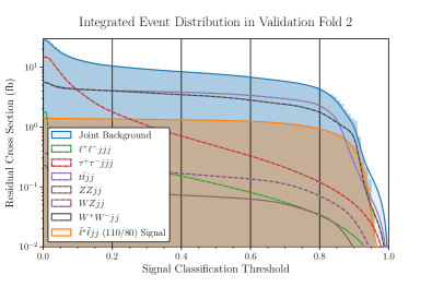
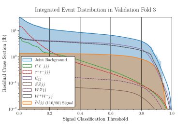
Figure 6: Same as Figure 1, but for different choices of training and evaluation samples. Plots illustrating the residual cross section for signal and background (as labeled) as a function of the BDT classification score after precuts.

Any event analyzed by the BDT is given a continuous decimal score between 0 and 1, with 1 being most signal-like and 0 being most background-like. In Figure 1, we plot the cross section for signal (orange) and background (as labeled) events to be classified with a score greater than a given threshold. Two similar plots made with a different choice of the training and evaluation samples are given in Appendix A (Figure 6). The far left of the plot (where the signal threshold is zero) corresponds to the case where the BDT results are ignored, and yield the cross section for the signal and each background to pass the precuts. The cross section for signal events to pass the precuts is $\sim 1.3~{}\rm fb$, indicating that, with an integrated luminosity of $\sim 300~{}\rm fb^{-1}$, $\sim 400$ signal events are expected to pass the precuts and be analyzed by the BDT. For each of the six backgrounds analyzed, the cross section for events to pass the precuts is in all cases $\lesssim 20~{}\rm fb$, with the largest cross section being for the $\bar{\tau}\tau jjj$ background. In particular, note that the $ZZjj$ and $WZjj$ backgrounds have been effectively eliminated by the precuts; the analysis of the BDT is largely irrelevant for those backgrounds, as $S/B\gg 1$ even before the BDT score is included.

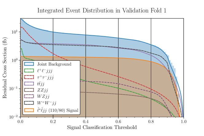
Figure 1: Plot illustrating the residual cross section for signal and background (as labeled) as a function of the BDT classification score after precuts. Corresponding plots for additional folds of training and evaluation samples can be found in Appendix A.

We classify an event as signal-like if its score exceeds a given a threshold, and as background-like if otherwise. Although more complicated methods which do not involve a binary assignment of signal-like or background-like status are possible [32, 33], we will find that this simple method is sufficient to provide substantial improvement in sensitivity.

IV.4 Results

Although the $\bar{\tau}\tau jjj$ background is the largest after the precuts, the BDT has little difficulty in discriminating this background from signal. For this background, as well as $\bar{\ell}\ell jjj$, the BDT can effectively suppress the background with little loss in signal cross section (see Figure 1, for a signal classification threshold $\gtrsim 0.4$). The greatest difficulty which the BDT finds is in discriminating the $\bar{t}tjj$ and $WWjj$ backgrounds from signal. We may thus expect that the competition between signal and the $\bar{t}tjj$ and $WWjj$ backgrounds will dominate our sensitivity (and associated signal to background ratio).

We see similarly from Figure 2 that the BDT provides a strong ability to discriminate signal from all backgrounds, though this discriminating power is weakest for the $\bar{t}tjj$ and $WWjj$ backgrounds. For the $\bar{t}tjj$ and $WWjj$ cases, although the BDT analysis exhibits good discriminating power, the large magnitude of these backgrounds relative to the signal cross section implies that, at best, the ratio of signal-to-background is ${\cal O}(1)$. This level of discrimination arises only when the signal classification threshold is high enough (see Figure 1) that only $\lesssim 150$ signal or background events are selected.

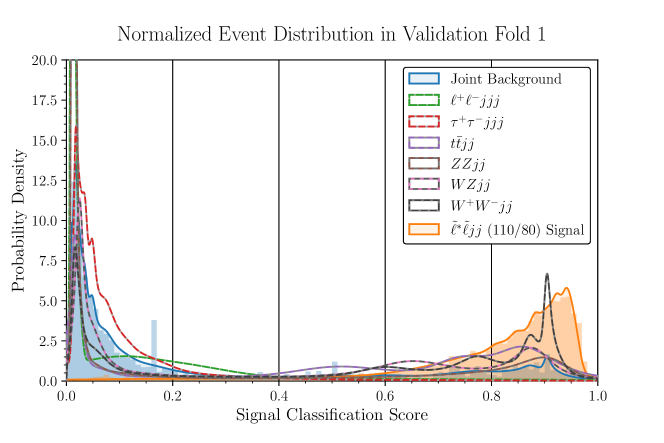
Figure 2: Density plot representing the separation of signal from each background (as labeled) by the boosted decision tree after precuts. For visual clarity, the densities are separately normalized such that the joint background density is not equivalent to the sum of the individual background densities. Corresponding plots for additional folds of training and evaluation samples can be found in Appendix A.

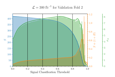
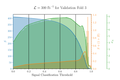
Figure 8: Same as Figure 3, but for different choices of training and evaluation samples. The number of signal events ($S$, blue), signal-to-background ration ($S\div(1+B)$, orange) and signal significance ($\sigma_{A}$, green) as a function of the signal classification threshold. Each curve represents an interpolation which smooths out the sharp features in the shaded region, which arise from small simulated event numbers.

We thus see that optimal performance of the BDT implies a reduction of background down to an event rate comparable to signal, with only a factor of $\sim 3$ reduction of the signal event rate. With $\sim 150$ signal events and $\sim 3$ times as many background events, one would expect that a sensitivity of $\gtrsim 6\sigma$ could be obtained with an $\sim 0.3$ signal to background ratio. This intuition is confirmed by the results of Figure 3, in which we present the number of signal events $S$ (blue), the signal-to-background ratio ($S\div(1+B)$, orange), and the signal significance ($\sigma_{A}$, green) as a function of the signal classification threshold, assuming an integrated luminosity of $300~{}\rm fb^{-1}$. Note that shaded regions show sharp features which arise when the number of simulated events which exceed the signal classification threshold is small, and can thus vary dramatically as the threshold increases. These sharp features arise when $S$ is small and do not represent reliable estimates, as they may be artifacts of the size of the simulated dataset. We instead focus on the solid curves, which represent an interpolation of the boundary of the shaded regions which smooths out these sharp features. In Appendix A, the two panels of Figure 8 present analyses with different choices of the sample used for training and evaluation. All three panels are roughly consistent, indicating that our result is robust to variations in the training set. In particular, for a signal classification threshold of $\sim 0.9$, we find that a scenario with $m_{\tilde{\ell}}=110~{}\,{\rm GeV}$, $m_{X}=80~{}\,{\rm GeV}$ can be detected with $\gtrsim 6\sigma$ significance and a signal-to-background ratio of $\sim 0.3$, with $S\sim 100$. This represents a marked improvement over the results obtained from the cut-based approach used in [3], in which only $3.0\sigma$ sensitivity (with a signal-to-background ratio of $0.2$) could be obtained with the same luminosity (see Table 3). Moreover, we see that using the cuts imposed in [3] as precuts, with subsequent signal classification by a BDT, does not provide significantly improved sensitivity. Evidently the cut-based approach used in this earlier analysis results in too a large reduction in the number of signal events for useful signal classification.

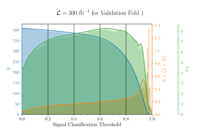
Figure 3: The number of signal events ($S$, blue), signal-to-background ration ($S\div(1+B)$, orange) and signal significance ($\sigma_{A}$, green) as a function of the signal classification threshold. Each curve represents an interpolation which smooths out the sharp features in the shaded region, which arise from small event numbers. Corresponding plots for additional folds of training and evaluation samples can be found in Appendix A.

Since the main work of the BDT (beyond the precuts, whose intuition we understand) is in rejecting the $\bar{t}tjj$ and $WWjj$ backgrounds, we can ask which kinematic variables the BDT used in that analysis. These results are shown in Figure 4 which indicate which kinematic variables dominate the “total gain”  when a BDT is trained only against a single background. This figure thus gives an indication of which variables are most useful in discriminating signal from a particular background. In particular, the most important kinematic variable for rejecting the $ttjj$ and $WWjj$backgrounds is $M_{\rm T2}^{100}$, which is defined, as in Ref. [24], as the minimal mass of a parent particle under the assumption that the parent particles are pair produced and each decays to a lepton and an invisible particle with a mass of $100\,{\rm GeV}$. Note that this variable was also used in the slepton search analysis presented in Ref. [1], though with a different purpose.

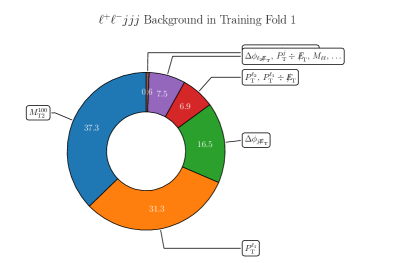
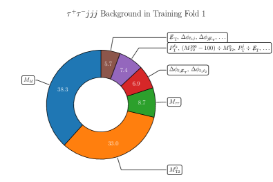
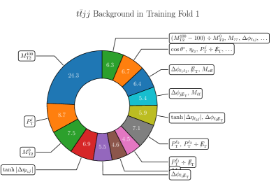
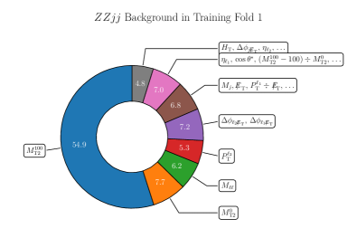
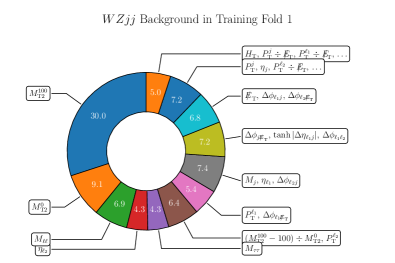
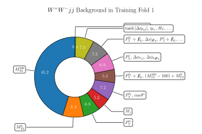
Figure 4: Plots indicating the relative importance of various kinematic features to the separation of signal from background by the boosted decision tree after level 1 pre-selections, respectively (left-to-right then top-to-bottom) for $\ell\ell jjj$, $\tau\tau jjj$, $t\bar{t}jj$, $ZZjj$, $WZjj$, and $WWjj$. Note that, in each panel, results are shown for a BDT which is trained only with signal and the particular background process in question.

The distributions of $M_{\rm T2}^{100}$ for signal and $\bar{t}tjj$ and $WWjj$ background events (after precuts) are given in Figure 5 We can see from these distributions that $M_{\rm T2}^{100}$ contributes significant ability to discriminate between signal and background. In particular, background events are biased towards higher values of $M_{\rm T2}^{100}$, since for background events, the invisible particles are neutrinos which are much lighter than the ansatz of $100\,{\rm GeV}$.

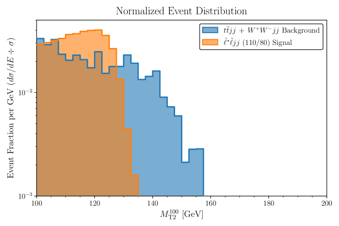
Figure 5: The distribution of $M_{T2}^{100}$ for events passing the precuts for signal (orange), as well as the combined $ttjj$ and $WWjj$ backgrounds (blue).

However, these distributions do not provide a clear sense of how $M_{\rm T2}^{100}$ is correlated with other variables, which is the type of information one would expect to be learned by a BDT. To consider this question, we assume that the only relevant background processes are $ttjj$ and $WWjj$. That is, we ignore the $WZjj$ and $ZZjj$ background classes (which are essentially eliminated by the precuts) and the $\mu\mu jjj$ and $\tau\tau jjj$ background classes (which are easily eliminated by the BDT). After the precuts, we see from Figure 2 that we are left with $\sim 400$ signal events, and $\sim 3300$ background, roughly evenly split between $ttjj$ and $WWjj$. We then consider a simple cut in which we accept only events with $M_{\rm T2}^{100}<130\,{\rm GeV}$. This cut admits almost all signal events, but reduces each class of background events by roughly 1/3. This simple cut-and-count analysis would yield a signal-to-background ratio of $S/B\sim 0.18$, with a signal significance of $\sim 8.5\sigma$. Indeed, we see that a 1/3 reduction in background, with a small reduction in signal, is roughly what the BDT achieves with a signal classification threshold set at $\sim 0.6$ (see Figure 1), yielding approximately the significance and signal-to-background ratio we estimated with a cut-and-count analysis (see Figure 3). The deeper correlations found by the BDT (at least in regard to the $ttjj$ and $WWjj$ backgrounds) lead to an improvement in the signal-to-background ratio of roughly a factor of 2 as the signal classification threshold is raised to $>0.9$.

Since the imposition of a simple cut such as $M_{\rm T2}^{100}<130\,{\rm GeV}$ seems to replicate at least part of the BDT analysis, one might ask if imposing this as a precut could improve the performance of the BDT, by allowing it to focus on less obvious correlations. To test this possibility, we ran a second analysis in which $M_{\rm T2}^{100}<130\,{\rm GeV}$ was imposed as a additional precut. The results are fairly similar to analysis without this additional precut (see Table 3). It appears that, because the $ttjj$ and $WWjj$ backgrounds are not excessively large compared to the other backgrounds and are within an order of magnitude of the signal, after applying the precuts described in Section IV.3, the BDT was not overly focused on reducing them, and thus did not gain significantly in performance when the $ttjj$ and $WWjj$ backgrounds were reduced through an additional precut.

Event Selection	This work		This work $+$ $M_{\rm T2}^{100}<130\,\,{\rm GeV}$		Intermediate mass gaps in [3]
	Precuts	BDT	Precuts	BDT	Precuts	BDT
BDT signal threshold	-	$0.47-0.90$	-	$0.34-0.88$	-	$0.00-0.71$
Events at $\mathcal{L}=300\,\rm fb^{-1}$	$413$	$107-386$	$405$	$121-387$	$48$	$26-51$
$S\div(1+B)$	$0.05$	$0.15-0.36$	$0.06$	$0.15-0.31$	$0.20$	$0.18-0.35$
$\sigma_{A}$	$4.4$	$5.8-8.2$	$4.8$	$5.6-8.2$	$3.0$	$2.5-3.7$

Table 3: Summary of results for our benchmark mass spectrum (i.e. $m_{\tilde{\ell}}=110\,\,{\rm GeV}$ and $m_{\tilde{\ell}}-m_{X}=30\,\,{\rm GeV}$) after implementing different event selections. For each set of precuts, we show the number of signal events, the signal to background ratio and the signal sensitivity both before and after application of the BDT. When only considering the precuts, we average the respective metrics between the 3 folds of the data. In contrast, the respective BDT signal score thresholds are optimized to show as broad a range of $\sigma_{A}$ possible between the different folds while maintaining $S\div(1+B)\geq 0.15$. The first event selection summarizes the the results of the event selection with precuts described in Section IV.3. The second event selection adds a precut on $M_{\rm T2}^{100}$ and the third event selection implements precuts corresponding to that which is implemented for the intermediate mass gap scenarios in previous work [3]. Note the average number of events after precuts between all 3 folds of the data in this final event selection is smaller that the upper end of the range of numbers of signal events after application of the BDT because of the variation between folds at a signal score threshold of 0.00, which is equivalent to only applying the precuts.

	$m_{\tilde{\ell}}=110\,\,{\rm GeV}$		$m_{\tilde{\ell}}=160\,\,{\rm GeV}$		$m_{\tilde{\ell}}=300\,\,{\rm GeV}$
	Benchmark	Retrained	Benchmark	Retrained	Benchmark	Retrained
$\Delta m=30\,\,{\rm GeV}$	$0.47-0.90$	-	$0.91-0.92$	$0.90-0.94$	-	-
	$107-386$	-	$33-55$	$13-43$	-	-
	$0.15-0.36$	-	$0.18-0.32$	$0.15-0.39$	$<0.15$	$<0.15$
	$5.8-8.2$	-	$2.5-3.1$	$1.8-2.9$	-	-
$\Delta m=40\,\,{\rm GeV}$	$0.47-0.91$	$0.23-0.87$	-	$0.90-0.92$	-	-
	$68-375$	$163-496$	-	$24-49$	-	-
	$0.15-0.36$	$0.15-0.35$	$<0.15$	$0.15-0.25$	$<0.15$	$<0.15$
	$4.2-7.9$	$6.7-9.1$	-	$1.9-3.0$	-	-
$\Delta m=50\,\,{\rm GeV}$	$0.59-0.90$	$0.13-0.88$	-	$0.79-0.93$	-	-
	$67-320$	$172-575$	-	$38-156$	-	-
	$0.15-0.23$	$0.15-0.42$	$<0.15$	$0.15-0.35$	$<0.15$	$<0.15$
	$3.7-7.3$	$7.6-10.7$	-	$3.0-5.4$	-	-
$\Delta m=60\,\,{\rm GeV}$	$0.62-0.90$	$0.05-0.90$	-	$0.54-0.96$	-	$0.96$
	$60-295$	$252-691$	-	$21-273$	-	$14-16$
	$0.15-0.21$	$0.15-1.01$	$<0.15$	$0.15-1.16$	$<0.15$	$0.15-0.26$
	$3.3-6.9$	$9.9-14.9$	-	$3.6-7.9$	-	$1.5-1.9$

Table 4: Summary of results for a variety of different mass spectra. For each combination of scalar mass $m_{\tilde{\ell}}$ and mass splitting $\Delta m=m_{\tilde{\ell}}-m_{X}$, we show (from top to bottom) the optimal signal score threshold for the BDT, the number of signal events expected at $\mathcal{L}=300\,\rm fb^{-1}$, $S\div(1+B)$ and $\sigma_{A}$. For each case, we test the BDT trained on the benchmark spectrum (i.e. $m_{\tilde{\ell}}=110\,\,{\rm GeV}$ and $\Delta m=30\,\,{\rm GeV}$) and the BDT retrained specifically for each spectrum. The respective BDT signal score thresholds are optimized to show as broad a range of $\sigma_{A}$ possible while maintaining $S\div(1+B)\geq 0.15$.

IV.5 Other Benchmarks

Until now, we have considered a single benchmark parameter point: $m_{\tilde{\ell}}=110~{}\,{\rm GeV}$, $m_{X}=80~{}\,{\rm GeV}$. Here we consider the sensitivity of an LHC search with $300~{}\rm fb^{-1}$ integrated luminosity to models with different choices for the masses. In Table 4, we consider $m_{\tilde{\ell}}=110,160,300~{}\,{\rm GeV}$, with $m_{\tilde{\ell}}-m_{X}=30,40,50,60~{}\,{\rm GeV}$. In each case, we either use BDT trained against the original benchmark model, or against the model to be analyzed (in all cases, the original precuts are used). For each analysis, we present an optimal range for the signal classification thresholds, and the range of the number of signal events, signal to background ratio, and signal significance as one varies the signal classification threshold within its optimal range. We only present results for $S\div(1+B)\geq 0.15$, in order to ensure that the analysis is robust against likely systematic uncertainties [1, 15].

For cases with $m_{\tilde{\ell}}=110~{}\,{\rm GeV}$ and larger mass gaps, $m_{\tilde{\ell}}-m_{X}>30~{}\,{\rm GeV}$, we see that the BDT trained on the benchmark spectrum, $m_{\tilde{\ell}}=110~{}\,{\rm GeV}$ and $m_{\tilde{\ell}}-m_{X}=30~{}\,{\rm GeV}$, maintains robust sensitivity to scalar muon production even with some degradation as the mass gaps become larger. Alternatively, when training the BDT individually for each benchmark, we see that the sensitivity is enhanced at larger mass splittings due to the improved separation of signal from background in the kinematic distributions. Although mass gaps $m_{\tilde{\ell}}-m_{X}=50,60~{}\,{\rm GeV}$ are currently excluded for $m_{\tilde{\ell}}=110~{}\,{\rm GeV}$, the signal significance we project for the BDT analysis of these cases is considerably larger than in the most stringent LHC constraints from Ref. [1], which exclude mass splittings of $\sim 50~{}\,{\rm GeV}$ at $\sim 2\sigma$. Similar dependencies of the sensitivity in the BDT analysis on the mass splitting can be seen for $m_{\tilde{\ell}}=160~{}\,{\rm GeV}$, however the BDT trained on the benchmark mass spectrum is only sensitive to the scenario with the same mass splitting of $m_{\tilde{\ell}}-m_{X}=30~{}\,{\rm GeV}$. When the BDT is retrained for each mass spectrum, we see the BDT could be sensitive to the full range of mass splittings from $30~{}\,{\rm GeV}$ to $60~{}\,{\rm GeV}$, none of which are currently constrained by LHC searches.

For $m_{\tilde{\ell}}=300~{}\,{\rm GeV}$, we never find $S\div(1+B)$ much larger than $0.15$, implying that a BDT search using these precuts might be difficult even at higher luminosity. But it is worth nothing that, for such a large lepton partner mass, the cross section for signal events to pass the precuts is much smaller than each of the backgrounds, with the total background well over two orders of magnitude larger than the signal, after imposing the precuts. The precuts were imposed precisely to eliminate this hierarchy, and we see that the precuts chosen to be adequate for $m_{\tilde{\ell}}=110~{}\,{\rm GeV}$ do not achieve this purpose if the lepton partner mass is much heavier. Better prospects would likely lie in developing more aggressive precuts to study this higher mass range (likely using higher luminosity), but that is beyond the scope of this work. In particular, training a BDT after the imposition of more aggressive precuts would likely require a much larger sample of simulated events.

V Conventional Wisdom for BDTs

There are several lessons that have been learned during the course of this study that would seem to represent a type of conventional wisdom which is substantially transferable in other similar applications.

The approach described in Section II works reasonably well “out of the box,” but we have observed that it is possible to achieve significantly better separation between signal and background using a hybrid technique that involves significant human input in conjunction with training of the BDT. By contrast, the emerging understanding in the deep-learning community is that one should generally just “get out of the way” and let the training proceed with minimal supervision and data curation. However, that intuition is apparently less applicable in the context of more basic types of machine learning applications such as boosted decision trees. The upside is that this additional investment of effort comes with a very substantially expanded and auditable inventory of precisely what and how the machine was learning, while still typically accessing a level of feature separation that meaningfully exceeds what is available with manual feature selections after maximal effort.

In a similar vein, the BDT seems to take maximal advantage of high-level features that have been constructed to efficiently encode physics features that are expected to be relevant. Again, by contrast, deep-learning approaches are known to work exceptionally well on raw low-level data, and extensive human curation is generally not necessary, or may even be detrimental. This is because a neural network of sufficient complexity can essentially mimic any mathematical transformation, and training will drive the development of this function in an optimized way. By contrast, shallow decision trees are always splitting on single features, and they tend to operate most effectively when the available features are preconfigured to very densely encode the most relevant parameterization of available information. For example, we generally find that reconstructed masses and composite constructions like $M_{\rm T2}$ or $\cos\theta^{*}$ pack much more punch than isolated kinematic features. Even simple operations, like taking differences or ratios of scales or angular coordinates that are expected to have more discriminating power as relative values than absolute values can increase efficiency.

Additionally, a very deep layer of background will be quite difficult for the BDT to “see through,” and it is helpful to remove “obvious” backgrounds prior to engaging the BDT. Along these lines, it is often the case that the most dominant backgrounds can be the simplest to defeat, and it seems that this should always be done up front when it is possible. For example, the cross section of single $Z$ events is extremely large, and its magnitude will typically overwhelm any search for final states that feature opposite-sign same-flavor dileptons. However, the vast majority of these dilepton events will cluster around the resonant $Z$ mass, and the residual cross section can be reduced dramatically with a simple window cut exclusion. Of course, the BDT can learn such a cut on its own. However, it seems to become “exhausted” in the process, and it becomes much harder for it to see the more subtle separations which are subsequently critical to achieving a successfully refined training if the dominant fraction of the input event weights are telling the BDT to pay attention to the mass window as a first priority. Not only should “obvious” discriminants be applied as manual precuts, it is advisable that the hardness of these cuts be selected so that the residual cross section associated with each type of background are brought approximately into parity.

On a related note, for practical reasons described previously, the starting cross section of signal events is always much smaller than that of relevant backgrounds. We find that the behavior of the BDT will be much more uniform and predictable if one separately normalizes the sum of signal and background weights to unity prior to training. This is because several of the hyperparameters associated with the BDT implementation, in particular those associated with regulation of the objective, have extensive (rather than intensive) scaling properties. This normalization helps to ensure that intuition developed regarding useful settings of these parameters has improved cross-applicability to other contexts. In fact, useful hyperparameter values generically tend to be “order one” in this normalization. Of course, one must then rescale back to physical cross sections when making predictions for rates in a real world experimental environment.

Since we are only really interested here in classification of categories that are somewhat difficult to separate by elementary means, the BDT will presumably need to access rather narrow and subtle features in order to train successfully. Likewise, since we are only really interested in enhancing the visibility of extremely rare processes, it is necessary to filter away the vast majority of competing background processes. These realities would appear to usher in a fundamental dilemma common to all relevant classification problems in collider physics. This is that the training is only successful in the regime where it has become statistically limited, and therefore less reliable. In other words, “harder cuts” leave fewer events, and it becomes successively more difficult to validate that the selected cuts are generalizable. This concern must be balanced against the priorities identified previously, such that any precuts will not preclude effective training. Specifically, there must be a statistically significant sampling of events on hand for the BDT to process. Of course, if it is possible to reduce all relevant background via manual selections, then it may not be necessary to further employ machine learning at all. However, overly aggressive precuts can additionally prevent the BDT from acting in a more surgical manner, and potentially achieving comparable background reductions while retaining a greater density of signal. Although the BDT is technically classifying rather than cutting, the same dilemma ultimately applies to its training process as well, and one often in practice contemplates an effective selection cut on some threshold of the resulting classification score.

VI Conclusion

We have considered the LHC sensitivity to a scenario of scalar lepton partner pair-production, with each partner decaying to a muon and an invisible particle with an intermediate mass splitting ($m_{\tilde{\ell}}-m_{X}\sim 30~{}\,{\rm GeV}$). This is a scenario for which current LHC sensitivity has not exceeded LEP, owing to the large electroweak background. We have used an analysis based on a boosted decision tree (BDT), and have found that with $300~{}\rm fb^{-1}$ luminosity, the LHC could achieve $\gtrsim 5\sigma$ sensitivity to currently allowed models ($m_{\tilde{\ell}}\sim 110~{}\,{\rm GeV}$), with a signal to background ratio $\gtrsim 0.3$. The BDT analysis could also exclude spectra with larger mass gaps $m_{\tilde{\ell}}-m_{X}\sim 50~{}\,{\rm GeV}$ and the same scalar mass with a significance $\lower 3.01385pt\hbox{$\;\stackrel{{\scriptstyle\textstyle>}}{{\sim}}\;$}4$ times larger than the most recent LHC analysis. With the same luminosity, LHC could exclude models with $m_{\tilde{\ell}}$ as large as $160~{}\,{\rm GeV}$. But for a larger mass splitting ($\sim 60~{}\,{\rm GeV}$), the LHC could provide $>5\sigma$ evidence for models with $m_{\tilde{\ell}}\sim 160~{}\,{\rm GeV}$ (also allowed by analyses of current data). Thus, a boosted decision tree analysis in scalar lepton partner searches could definitively probe realizations of the MSSM in which scalar muon mediated interactions can both deplete the relic density through dark matter annihilation and account for the anomalous magnetic moment of the muon.

The most difficult backgrounds to discriminate are $\bar{t}t~{}{\rm and}~{}WW~{}+$ jets. The kinematic variable relied on most heavily by the BDT in discriminating signal from these background is $M_{\rm T2}^{100}$. Nevertheless, the BDT makes good use of less obvious variables to simultaneously suppress the $\mu\mu~{}+$ jets and $\tau\tau~{}+$ jets backgrounds while further reducing $\bar{t}t~{}{\rm and}~{}WW~{}+$ jets, producing an optimal signal-to-background ratio which is a factor of $\sim 6$ better than one would get by simply imposing an additional cut on $M_{\rm T2}^{100}$.

In performing this analysis, we have learned several lessons regarding the application of BDTs to LHC analyses which may be applied to other searches. In particular, we found that the BDT is much more effective if obvious precuts are applied which reduce each surviving background to roughly equal event numbers, so that the BDT is not overly dominated by any one background class. Essentially, there is little gained by having a BDT relearn things we already know. On the other hand, while the imposition of precuts which reduce very large backgrounds improves the BDT performance, the application of even obvious precuts which have the effect of removing backgrounds which are only comparable to the signal has little effect on the BDT’s performance.

There any many avenues open for further study. In particular, it would be interesting to explore the optimal tradeoff between using precuts to reduce backgrounds before the application of a BDT, as opposed to simply allowing a BDT to analyze as large a data set as possible. It would also be interesting to investigate other approaches to the problem of backgrounds with widely disparate cross sections, such as changes to the BDT hyperparameters.

We have found that it is difficult to properly train a BDT if the most difficult backgrounds to remove are swamped by larger (though more tractable) backgrounds. The essential problem is that the simulation data which one uses for training are necessarily only a fraction of the vast LHC dataset. A subleading background may be undersampled, leading a BDT to focus its training on quirks of the training set, rather than robust features. But this is a more general danger which could prove challenging for similar applications of other machine learning techniques. It is difficult to ensure that the toughest backgrounds are sufficiently well sampled in simulation if one has not already characterized the backgrounds which are easy or difficult to discriminate. It would be interesting to explore the importance of sufficient background sampling in the training of deep learning algorithms such as neural networks.

Our analysis has in a sense been optimized for the intermediate mass gap range, as we have trained the BDT with a single BSM model with mass splitting of $30\,{\rm GeV}$. Unsurprisingly, a BDT trained on only this BSM model does far worse at identifying the presence of new physics if the mass splitting is either significantly larger or smaller, because of the changes to the underlying features of the kinematic distributions which drive this sensitivity (see, for example [3]). It would be interesting to train a BDT with a range of mass splittings, to determine the trade-off between efficiency and generality of the analysis. In connection with this question, it would also be interesting to consider alternative choices in the training procedure. For example, one could consider training BDTs separately to distinguish signal from each of the leading backgrounds, with the individual scores combined to yield an overall signal classifier. In this work, we used a signal classifier threshold to make a binary classification of an event as either signal or background, but it would be interesting to consider alternative approaches.

Acknowledgements We are grateful to Alexander Khanov, Xerxes Tata and Evelyn Thomson for useful discussions. We thank Jordan Pittman, Stephanie Samperio, Conrad Albrecht, and Joseph Hansen for technical assistance. For facilitating portions of this research, B. Dutta, J. Kumar and J.W. Walker wish to acknowledge the Center for Theoretical Underground Physics and Related Areas (CETUP*), The Institute for Underground Science at Sanford Underground Research Facility (SURF), and the South Dakota Science and Technology Authority for hospitality and financial support, as well as for providing a stimulating environment. B. Dutta is supported in part by DOE Grant DE-SC0010813. T. Ghosh is supported by the funding available from the Department of Atomic Energy (DAE), Government of India for Harish-Chandra Research Institute (HRI). J. Kumar would like to thank the organizers of SUSY 2023 for their hospitality. J. Kumar is supported in part by DOE grant DE-SC0010504. P. Sandick is supported in part by NSF grant PHY-2014075. P. Stengel would like to thank the organizers of Cosmology 2023 in Miramare for their hospitality. P. Stengel is funded by the Instituto Nazionale di Fisica Nucleare (INFN) through the project of the InDark INFN Special Initiative: “Neutrinos and other light relics in view of future cosmological observations” (n. 23590/2021). J.W. Walker is supported in part by the National Science Foundation under Grant NSF PHY-2112799.

Appendix A Additional Validation Folds

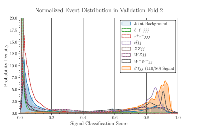
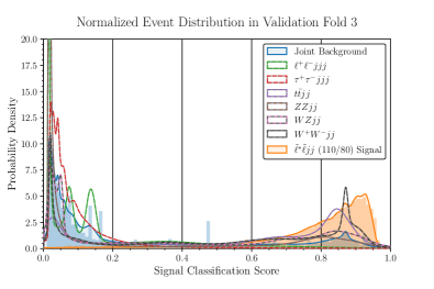
Figure 7: Same as Figure 2, but for different choices of training and evaluation samples. Density plots representing the separation of signal from each background (as labeled) by the boosted decision tree after precuts. For visual clarity, the densities are separately normalized such that the joint background density is not equivalent to the sum of the individual background densities.

References

- [1] [ATLAS], “Search for direct pair production of sleptons and charginos decaying to two leptons and neutralinos with mass splittings near the -boson mass in TeV collisions with the ATLAS detector,” [arXiv:2209.13935 [hep-ex]].
- [2] LEPSUSYWG, ALEPH, DELPHI, L3, OPAL Collaborations, “Combined LEP Selectron/Smuon/Stau Results, 183-208 GeV,” LEPSUSYWG/04-01.1 (2004), URL: https://lepsusy.web.cern.ch/lepsusy/www/sleptons_summer04/slep_final.html.
- [3] B. Dutta, K. Fantahun, A. Fernando, T. Ghosh, J. Kumar, P. Sandick, P. Stengel and J. W. Walker, “Probing Squeezed Bino-Slepton Spectra with the Large Hadron Collider,” Phys. Rev. D 96, no.7, 075037 (2017) doi:10.1103/PhysRevD.96.075037 [arXiv:1706.05339 [hep-ph]].
- [4] P. Baldi, P. Sadowski and D. Whiteson, “Searching for Exotic Particles in High-Energy Physics with Deep Learning,” Nature Commun. 5, 4308 (2014) doi:10.1038/ncomms5308 [arXiv:1402.4735 [hep-ph]].
- [5] A. Dey, J. Lahiri and B. Mukhopadhyaya, “LHC signals of a heavy doublet Higgs as dark matter portal: cut-based approach and improvement with gradient boosting and neural networks,” JHEP 09, 004 (2019) doi:10.1007/JHEP09(2019)004 [arXiv:1905.02242 [hep-ph]].
- [6] C. K. Khosa, V. Sanz and M. Soughton, “Using machine learning to disentangle LHC signatures of Dark Matter candidates,” SciPost Phys. 10, no.6, 151 (2021) doi:10.21468/SciPostPhys.10.6.151 [arXiv:1910.06058 [hep-ph]].
- [7] E. Arganda, A. D. Medina, A. D. Perez and A. Szynkman, “Towards a method to anticipate dark matter signals with deep learning at the LHC,” SciPost Phys. 12, no.2, 063 (2022) doi:10.21468/SciPostPhys.12.2.063 [arXiv:2105.12018 [hep-ph]].
- [8] T. Finke, M. Krämer, M. Lipp and A. Mück, “Boosting mono-jet searches with model-agnostic machine learning,” JHEP 08, 015 (2022) doi:10.1007/JHEP08(2022)015 [arXiv:2204.11889 [hep-ph]].
- [9] B. M. Dillon, R. Mastandrea and B. Nachman, “Self-supervised anomaly detection for new physics,” Phys. Rev. D 106, no.5, 056005 (2022) doi:10.1103/PhysRevD.106.056005 [arXiv:2205.10380 [hep-ph]].
- [10] V. K. MB, A. K. Nayak and A. K. Radhakrishnan, “Invariant mass reconstruction of heavy gauge bosons decaying to leptons using machine learning techniques,” [arXiv:2304.01126 [hep-ph]].
- [11] T. Ghosh, C. Kelso, J. Kumar, P. Sandick and P. Stengel, “Simplified dark matter models with charged mediators,” [arXiv:2203.08107 [hep-ph]].
- [12] K. Fukushima, C. Kelso, J. Kumar, P. Sandick and T. Yamamoto, “MSSM dark matter and a light slepton sector: The Incredible Bulk,” Phys. Rev. D 90, no.9, 095007 (2014) doi:10.1103/PhysRevD.90.095007 [arXiv:1406.4903 [hep-ph]].
- [13] J. T. Acuña, P. Stengel and P. Ullio, “Minimal dark matter model for muon g-2 with scalar lepton partners up to the TeV scale,” Phys. Rev. D 105, no.7, 075007 (2022) doi:10.1103/PhysRevD.105.075007 [arXiv:2112.08992 [hep-ph]].
- [14] J. T. Acuña, P. Stengel and P. Ullio, “Neutron Star Heating in Dark Matter Models for Muon g-2 with Scalar Lepton Partners up to the TeV Scale,” [arXiv:2209.12552 [hep-ph]].
- [15] G. Aad et al. [ATLAS], “Searches for electroweak production of supersymmetric particles with compressed mass spectra in 13 TeV collisions with the ATLAS detector,” Phys. Rev. D 101, no.5, 052005 (2020) doi:10.1103/PhysRevD.101.052005 [arXiv:1911.12606 [hep-ex]].
- [16] J. Alwall, R. Frederix, S. Frixione, V. Hirschi, F. Maltoni, O. Mattelaer, H. S. Shao, T. Stelzer, P. Torrielli and M. Zaro, “The automated computation of tree-level and next-to-leading order differential cross sections, and their matching to parton shower simulations,” JHEP 07, 079 (2014) doi:10.1007/JHEP07(2014)079 [arXiv:1405.0301 [hep-ph]].
- [17] T. Sjöstrand, S. Ask, J. R. Christiansen, R. Corke, N. Desai, P. Ilten, S. Mrenna, S. Prestel, C. O. Rasmussen and P. Z. Skands, “An introduction to PYTHIA 8.2,” Comput. Phys. Commun. 191, 159-177 (2015) doi:10.1016/j.cpc.2015.01.024 [arXiv:1410.3012 [hep-ph]].
- [18] J. de Favereau et al. [DELPHES 3], “DELPHES 3, A modular framework for fast simulation of a generic collider experiment,” JHEP 02, 057 (2014) doi:10.1007/JHEP02(2014)057 [arXiv:1307.6346 [hep-ex]].
- [19] [ATLAS], “Tagging and suppression of pileup jets,” ATLAS-CONF-2014-018.
- [20] J. W. Walker, “AEACuS, RHADAManTHUS, and MInOS: Automated Tools for Collider Event Analysis, Plotting, and Machine Learning,” (2023), https://github.com/joelwwalker/AEACuS
- [21] J. Walker, “Automated Collider Event Selection, Plotting, & Machine Learning with AEACuS, RHADAManTHUS, & MInOS,” PoS CompTools2021, 027 (2022) doi:10.22323/1.409.0027
- [22] A. Barr, ”Measuring slepton spin at the LHC,” JHEP 0602, 042 (2006) doi:10.1088/1126-6708/2006/02/042 [arXiv:hep-ph/0511115].
- [23] K. Matchev, et al., ”Measuring slepton spin at the LHC,” doi:10.1007/JHEP11(2012)006 [arXiv:1205.2054].
- [24] C. G. Lester and D. J. Summers, “Measuring masses of semiinvisibly decaying particles pair produced at hadron colliders,” Phys. Lett. B 463, 99-103 (1999) doi:10.1016/S0370-2693(99)00945-4 [arXiv:hep-ph/9906349 [hep-ph]].
- [25] H. C. Cheng and Z. Han, “Minimal Kinematic Constraints and m(T2),” JHEP 12, 063 (2008) doi:10.1088/1126-6708/2008/12/063 [arXiv:0810.5178 [hep-ph]].
- [26] A. J. Barr, B. Gripaios and C. G. Lester, “Transverse masses and kinematic constraints: from the boundary to the crease,” JHEP 11, 096 (2009) doi:10.1088/1126-6708/2009/11/096 [arXiv:0908.3779 [hep-ph]].
- [27] Z. Han and Y. Liu, “MT2 to the Rescue – Searching for Sleptons in Compressed Spectra at the LHC,” Phys. Rev. D 92, no.1, 015010 (2015) doi:10.1103/PhysRevD.92.015010 [arXiv:1412.0618 [hep-ph]].
- [28] R. K. Ellis, I. Hinchliffe, M. Soldate and J. J. van der Bij, “Higgs Decay to tau+ tau-: A Possible Signature of Intermediate Mass Higgs Bosons at the SSC,” Nucl. Phys. B 297, 221 (1988). doi:10.1016/0550-3213(88)90019-3 .
- [29] [ATLAS], “Trigger menu in 2018,” ATL-DAQ-PUB-2019-001.
- [30] T. Chen and G. Carlos, “XGBoost: A Scalable Tree Boosting System,” Proceedings of the 22nd ACM SIGKDD International Conference on Knowledge Discovery and Data Mining, 785–-794 (2016).
- [31] J.D. Hunter, “Matplotlib: A 2D graphics environment,” Computing in Science & Engineering 9, no.3, 90–95 (2007).
- [32] S. Whiteson and D. Whiteson, “Machine Learning for Event Selection in High Energy Physics,” Eng. Appl of AI (22) 1203-1212 Dec. 2023, doi:10.1016/j.engappai.2009.05.004.
- [33] C. W. Murphy, “Class Imbalance Techniques for High Energy Physics,” SciPost Phys. 7, no.6, 076 (2019) doi:10.21468/SciPostPhys.7.6.076 [arXiv:1905.00339 [hep-ph]].
- [34] G. Cowan, K. Cranmer, E. Gross and O. Vitells, “Asymptotic formulae for likelihood-based tests of new physics,” Eur. Phys. J. C 71, 1554 (2011) [erratum: Eur. Phys. J. C 73, 2501 (2013)] doi:10.1140/epjc/s10052-011-1554-0 [arXiv:1007.1727 [physics.data-an]].