The One-hundred-deg² DECam Imaging in Narrowbands (ODIN): Survey Design and Science Goals

Abstract

We describe the survey design and science goals for ODIN (One-hundred-deg² DECam Imaging in Narrowbands), a NOIRLab survey using the Dark Energy Camera (DECam) to obtain deep (AB$\sim$25.7) narrow-band images over an unprecedented area of sky. The three custom-built narrow-band filters, $N419$, $N501$, and $N673$, have central wavelengths of 419, 501, and 673 nm and respective full-width-at-half-maxima of 7.2, 7.4, and 9.8 nm, corresponding to Ly$\alpha$ at $z=$2.4, 3.1, and 4.5 and cosmic times of 2.8, 2.1, and 1.4 Gyr, respectively. When combined with even deeper, public broad-band data from Hyper Suprime-Cam, DECam, and in the future, LSST, the ODIN narrow-band images will enable the selection of over 100,000 Ly$\alpha$-emitting (LAE) galaxies at these epochs. ODIN-selected LAEs will identify protoclusters as galaxy overdensities, and the deep narrow-band images enable detection of highly extended Ly$\alpha$ blobs (LABs). Primary science goals include measuring the clustering strength and dark matter halo connection of LAEs, LABs, and protoclusters, and their respective relationship to filaments in the cosmic web. The three epochs allow the redshift evolution of these properties to be determined during the period known as Cosmic Noon, where star formation was at its peak. The narrow-band filter wavelengths are designed to enable interloper rejection and further scientific studies by revealing [O ii] and [O iii] at $z=0.34$, Ly$\alpha$ and He ii 1640 at $z=3.1$, and Lyman continuum plus Ly$\alpha$ at $z=4.5$. Ancillary science includes similar studies of the lower-redshift emission-line galaxy samples and investigations of nearby star-forming galaxies resolved into numerous [O iii] and [S ii] emitting regions.

1 Introduction

In the hierarchical theory of structure formation, initial density fluctuations grow via gravitational instabilities and form filaments, sheets, voids, and collapsed halos (Bond et al., 1996). These features are collectively referred to as large-scale structures (LSS). In this picture, a galaxy’s fate is primarily determined by the surrounding LSS, which controls the rate and the timeline of gas accretion and feedback processes, as well as the likelihood of galaxy-galaxy interaction.

Observational evidence supporting this expectation is abundant. At physical scales of $\approx$100’s kpc, galaxies with a close companion tend to have enhanced star formation rates (SFRs) and follow a different mass-metallicity relation than that for isolated ‘field’ galaxies (e.g., Ellison et al., 2008; Hwang et al., 2011). At cluster scales ($\lesssim 1$ Mpc), the shape of the galaxy stellar mass function in cluster environment differs from that of average field (e.g., Baldry et al., 2006) in that fewer low-mass star-forming galaxies and a higher fraction of quenched galaxies are present. Similar trends persist in group-scale environments and in high-redshift ($z\approx 1$) clusters (Yang et al., 2009; Peng et al., 2010; van der Burg et al., 2020). Such environmental dependence may begin at $z\gtrsim 2$ (Lemaux et al., 2022), i.e., well before a large cosmic structure becomes fully virialized. At the largest scales (up to $\approx$10 Mpc comoving), the degree of galaxy clustering is a strong function of stellar mass, SFR, luminosity, and spectral type (e.g., Norberg et al., 2002; Adelberger et al., 2005; Giavalisco & Dickinson, 2001; Lee et al., 2006), suggesting that galaxies with larger stellar masses, higher SFR, and/or redder colors are hosted by more massive halos than their less massive, bluer counterparts.

At $z\gtrsim 2$, when the global star formation activity reached its peak (Madau & Dickinson, 2014), the role of the LSS environment in galaxy formation remains under-explored. Many of the strong spectral features redshift to the infrared wavelength, making ground-based investigations difficult. Moreover, severe cosmological dimming requires long integrations on large-aperture telescopes to detect continuum emission and measure redshift even for relatively bright galaxies, rendering a complete spectroscopic survey unfeasible. While the James Webb Space Telescope (JWST) and 30m-class telescopes will certainly alleviate these challenges, the small field of view probed by these facilities (typically, a few arcminutes on a side) is better suited for detailed follow-up studies of a few interesting systems rather than for general exploratory surveys large enough to probe the LSS.

At high redshift, Ly$\alpha$ emission provides one of the primary windows into the high-redshift universe (see review by Ouchi et al., 2020, and references therein), as it traces ionized and/or excited gas from star formation, black hole activity, and the gravitational collapse of dark matter halos. The Ly$\alpha$ emission strength from $z>2$ galaxies is inversely correlated with stellar mass and internal extinction, meaning that Ly$\alpha$ emitters (LAEs) tend to have younger ages and lower SFRs than continuum-selected galaxies (e.g., Gawiser et al., 2006; Guaita et al., 2011). They are also less dusty than any other known galaxy population (Weiss et al., 2021). Given the relative ease of narrow-band imaging compared to spectroscopy and the reduced projection effects of narrow- versus broad-band selection, LAEs are the most efficient tracer of the underlying matter distribution at high redshift. The utility of LAEs for this purpose has been known for two decades (e.g., Hu & McMahon, 1996; Ouchi et al., 2003; Kovač et al., 2007; Gawiser et al., 2007). Angular clustering measurements suggest that LAEs are hosted by moderate-mass halos (Gawiser et al., 2007; Guaita et al., 2010; Lee et al., 2014). These traits give LAEs the lowest clustering bias among visible tracers of the underlying matter distribution. Finally, Ly$\alpha$ mapping via narrow-band imaging offers an efficient alternative for collecting large galaxy samples in a well-defined volume with minimal contamination from foreground sources. The redshift precision, $\Delta z\sim 0.04-0.06$ is several times better than that afforded by the best photometric redshifts that can be derived using broad-band filters ($\Delta z\sim 0.1-0.2$ at $z>2$).

This paper is organized as follows. In Section 2, we describe the key science goals of the ODIN survey and provide a broad context and an overview of each topic. Section 3 summarizes the survey parameters, detailing the filter transmission, and the key characteristics of the survey fields; additionally, we justify the imaging depths and present the expected outcomes upon completion of the survey. In Section 4, we discuss the general procedures guiding the data acquisition and reduction, and in Section 5, we describe the survey’s existing and future data. Finally, in Section 6, we stress the legacy value of the ODIN data and the ODIN filters in advancing Galactic science. We adopt a $\Lambda$CDM concordance cosmology with $h=0.7$, $\Omega_{m}=0.27$, and $\Omega_{\Lambda}=0.73$ and use comoving distance scales unless noted otherwise. All magnitudes are in the AB scale (Oke & Gunn, 1983).

2 Primary ODIN Science Goals

The One-hundred-deg² DECam Imaging in Narrowbands (ODIN) is designed to enable a multitude of science goals but is primarily geared towards understanding the formation and evolution of galaxies in the distant universe. ODIN probes the large-scale structure in three narrow cosmic slices straddling the epoch of “Cosmic Noon” using custom-built narrow-band filters. These filters sample redshifted Ly$\alpha$ at cosmic ages of 2.8, 2.1, and 1.4 Gyr ($z=2.4$, 3.1, and 4.5), strategically placed to study the redshift evolution of galaxies and cosmic structures. When combined with the upcoming deep wide-field surveys to be conducted with the Rubin Observatory’s Legacy Survey of Space and Time (LSST), the Nancy Grace Roman telescope, and Euclid, ODIN has the potential to reveal the full diversity of astrophysical phenomena in the context of their LSS, as well as to measure the topology of LSS thereby constraining cosmological parameters. In what follows, we describe the primary goals of the ODIN survey.

2.1 Protoclusters, cosmic web, and galaxy inhabitants

Protoclusters are progenitors of the most massive gravitationally bound structures, i.e., clusters of galaxies. As such, protoclusters allow us to directly witness the formation and evolution of galaxies, thereby shedding light onto the physical processes that led to their early accelerated formation followed by strong and swift quenching that occurred at high redshift (e.g., Stanford et al., 1998; Blakeslee et al., 2003; Thomas et al., 2005; Eisenhardt et al., 2008; Mancone et al., 2010).

The limitations of studying protoclusters have been muti-fold: first, clean and statistically robust samples of protoclusters have been difficult to obtain. The lack of readily identifiable signatures – such as a hot intracluster medium and/or a concentration of quiescent galaxies – in young, yet-to-be-virialized structures of mostly star-forming galaxies leads to a strong reliance on spectroscopy for finding protoclusters. Photometric redshifts from broad- and intermediate-band filters can help with selection efficiency (e.g., Chiang et al., 2014), but few extragalactic fields have the data necessary to produce photo-z’s with the requisite $\Delta z\approx 0.1$ precision (e.g., Shi et al., 2019; Huang et al., 2022).

Second, protoclusters subtend tens of arcminutes in the sky (Muldrew et al., 2015; Chiang et al., 2013) making member identifications challenging. Even if the general region of a protocluster were targeted, blind spectroscopy would be dominated by fore- and background interlopers. Finally, massive clusters are very rare. The most massive, Coma-like clusters ($M_{\rm today}\gtrsim 10^{15}M_{\odot}$) have a space density of $\approx$180 Gpc^-3 (Reiprich & Böhringer, 2002), corresponding to $\approx$2.3 deg^-2 per unit redshift. Most surveys are ill-suited for discovering such sparsely distributed structures.

These difficulties explain why there are very few well-characterized protocluster systems (e.g. Dey et al., 2016; Cucciati et al., 2018). Despite the rapidly growing number of protoclusters and their candidates (e.g. Planck Collaboration et al., 2015; Toshikawa et al., 2018), there is a critical need for reliable markers or ‘signposts’ of protoclusters. Though possible candidates are numerous (see Overzier, 2016, and the references therein, but the candidates include radio galaxies, quasi-stellar objects, and Ly$\alpha$ nebulae), the extent of their success varies even when it can be measured. Moreover, the intersection of these markers, their respective selection biases, and their duty cycle (i.e., the typical timescale in which they stay visible) are currently unknown. Uniformly selected large samples of protoclusters are needed to address these questions.

ODIN uses LAE overdensities as tracers of massive cosmic structures. This is motivated by the fact that LAE samples suffer from much weaker projection effects than continuum-selected galaxies due to the narrow redshift interval and offer high sky density with contiguous coverage that cannot easily be achieved with spectroscopy. Additionally, studies of the few well-characterized protoclusters, such as SSA22, Hyperion, and PC217.9+32.3 (Steidel et al., 1999; Lee et al., 2014; Dey et al., 2016; Topping et al., 2018; Huang et al., 2022), suggest that LAEs trace the overall galaxy overdensity structures quite well, highlighting the systems’ filament-like structures and knots.

In this context, one of the immediate goals of ODIN in advancing protocluster science are to procure a statistically complete sample of protoclusters via the identification of low-mass, low-luminosity galaxies, and to explore the intersectionality with structures of dusty star-forming galaxies (e.g., Casey, 2016; Planck Collaboration et al., 2015), Lyman-break galaxies, extended Ly$\alpha$ nebulae, and radio galaxies. The survey volume and the target fields (Section 3) are chosen to allow robust, statistically significant comparisons of the samples. A first analysis of how the ODIN-selected Ly$\alpha$ nebulae are located in the context of LAE-traced cosmic filaments and protoclusters is provided in Ramakrishnan et al. (2023). The ODIN fields coincide with the regions with the deepest Spitzer IRAC data (Section 5.2), which will enable a systematic search for the progenitors of giant cluster ellipticals, some of which are expected to have already been formed at high redshift (e.g., Thomas et al., 2005; Mei et al., 2006). Deeper IR data from Roman in the next decade will push the limit further.

2.2 Extended Ly$\alpha$ nebulae

Extended Ly$\alpha$ nebulae, also known as Ly$\alpha$ “blobs” (LABs), emit Ly$\alpha$ radiation with total line luminosities of $10^{43}-10^{44}$ erg s^-1 on physical scales of 20–100 kpc (e.g., Francis et al., 1996; Steidel et al., 2000; Matsuda et al., 2004; Saito et al., 2006; Yang et al., 2009; Matsuda et al., 2011). This far exceeds the size of a single galaxy.

Given their extreme physical properties, the physical nature of LABs has astrophysical and cosmological implications. Some blobs are clearly produced by photoionization from intense radiation produced by embedded active galactic nuclei (AGN), which themselves may or may not be visible at optical wavelengths (e.g., Kollmeier et al., 2010; Overzier et al., 2013; Yang et al., 2014). The recombination of ionized gas results in Ly$\alpha$ photons, which resonantly scatter and illuminate the surrounding H i gas. In a few spectacular cases around luminous QSOs (e.g., Borisova et al., 2016; Arrigoni Battaia et al., 2019) or multiple AGN, the scattered Ly$\alpha$ emission reveals cosmic filaments connected to the source (e.g., Cantalupo et al., 2014; Umehata et al., 2019). Alternatively, Ly$\alpha$ photons produced in the star-forming regions of embedded galaxies may scatter outward and power LABs (e.g., Laursen & Sommer-Larsen, 2007; Cen & Zheng, 2013; Chang et al., 2023). Shock heating of the gas in the circumgalactic medium by starburst-driven superwinds has also been proposed as a possible mechanism (e.g., Taniguchi & Shioya, 2000).

Much attention has been given to LABs as potential signposts of gas accretion along cosmic filaments. As H i gas falls into the potential well of a dark matter halo and is heated to $\gtrsim 10^{4}$ K, a large fraction of the gravitational cooling radiation is expected to be emitted in Ly$\alpha$ (Haiman et al., 2000; Fardal et al., 2001). Although the tight correlation between stellar mass and SFRs, often referred to as the star-forming galaxy ‘main sequence’ (e.g., Noeske et al., 2007), implies that the dominant mode of galaxy growth is through a relatively smooth and prolonged inflow of gas, direct and clear evidence for this inflow has been challenging to obtain.

Recent ultradeep integral field observations suggest that some LABs may indeed be powered by gravitational cooling. Daddi et al. (2021) showed that the morphology and kinematics of the extended Ly$\alpha$ emission around a galaxy group at $z=2.91$ are consistent with gas inflow along multiple cosmic filaments converging onto the group. By studying extended Ly$\alpha$ emission around a handful of protoclusters or groups of galaxies, Daddi et al. (2022) reported tentative evidence that LAB luminosity correlates with dark matter halo mass (and thus with expected baryon accretion rate). These studies highlight the fact that direct detection of cold gas accretion near massive halos may be at the edge of the current observational reach.

Indeed, many known blobs are associated with galaxy overdensities (e.g., Shi et al., 2019) or lie near what appears to be a filament traced by galaxies (e.g., Erb et al., 2011). Prescott et al. (2008) surveyed the region surrounding a very luminous, mid-IR-detected blob (Dey et al., 2005) and reported an overdensity of galaxies (also see Xue et al., 2017). A Ly$\alpha$ survey around a known protocluster at $z=3.09$, SSA22, revealed multiple Ly$\alpha$ blobs (Steidel et al., 2000) residing in regions that appear to be converging filaments (Matsuda et al., 2004). Bădescu et al. (2017) noted that blobs tend to reside in the vicinity of protoclusters identified as LAE overdensities (also see Ramakrishnan et al., 2023). When combined with their high cosmic variance (Yang et al., 2010), the authors speculate that blobs may represent infalling proto-galaxy-groups.

To place definitive constraints on the physical origin(s) of LABs and their connection to cosmic structures, large and statistically complete samples of LABs are crucial. By detecting over 1,000 bright LABs at three cosmic epochs, ODIN will produce the largest blob sample to date and enable robust measurements of the sizes, and luminosities, and redshift evolution of these objects. Auto- and cross-correlation function measures will inform us of typical masses of LAB host halos and their interrelation with known cosmic structures. When combined with the ODIN protocluster samples, it will be possible to determine whether or not LABs are reliable tracers of protoclusters, which in turn constrains the duty cycle of the LAB phenomenon.

2.3 Physical properties of LAEs via LFs, SEDs, and Clustering

LAEs represent a low-dust, high specific star formation rate stage of galaxy evolution, possibly consistent with galaxies undergoing initial starbursts (Partridge & Peebles, 1967; Gawiser et al., 2007), making it important to fully characterize their properties. By detecting tens of thousands of LAEs situated in the wide and deep imaging fields in the equatorial and Southern sky, ODIN aims to greatly increase our knowledge of these galaxies’ physical properties.

With the rapid increase in sophistication of cosmological hydrodynamic simulations and semi-analytic models of galaxy formation, it has become possible to test theoretical predictions for the distribution of directly observed galaxy properties including their continuum and emission-line luminosities and colors. LAEs offer a unique probe of the low-mass bulk of the high-redshift galaxy distribution, but connecting them with these models requires matching the observed distribution of Ly$\alpha$ emission strengths i.e., the Ly$\alpha$ luminosity function (LF), which report the number density of LAEs as a function of their Ly$\alpha$ luminosity (e.g., Gronwall et al., 2007; Ciardullo et al., 2012; Sobral et al., 2018); the large statistical samples enabled by ODIN’s combination of depth and area and the strong interloper rejection enabled by deep photometry in multiple broad-band filters will yield improved LF measurements at each redshift.

Deep rest-UV-through-near-IR broadband photometry of LAEs available in the ODIN fields (Table 2) will enable improved Spectral Energy Distribution (SED) fitting to measure SFR, stellar masses, and dust extinction. Vargas et al. (2014) found that, with broad-band photometry significantly deeper than the narrow-band photometry used to select LAEs, it was not necessary to stack LAE SEDs in order to obtain robust parameter fits. Sufficiently deep $u$-band-through-IRAC photometry is available in the CANDELS (Nayyeri et al., 2017; Merlin et al., 2021) and COSMOS2020 (Weaver et al., 2021) catalogs. Shallower $ugrizyK$+IRAC SEDs are available for stacked SED analysis of $>$30,000 LAEs in the 24 deg² field of SHELA (Papovich et al., 2016; Wold et al., 2019; Stevans et al., 2021).

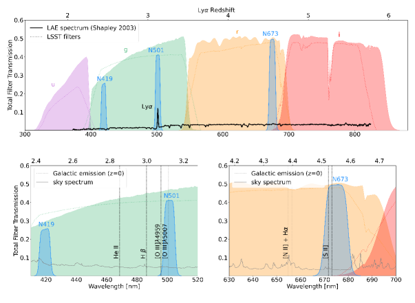
Figure 1: Top: The ODIN narrowband filters made for DECam (blue shaded regions; from left to right, $N419$, $N501$, and $N673$, respectively) together with the transmission curves for the broad-band filters from Subaru HSC ($gri$) and CFHT/MegaCam ($u$). Future LSST passbands for the same broad-bands are shown as dotted lines. These imaging data are combined to isolate redshifted Ly$\alpha$ emission falling into the narrowband filters as illustrated by the template LAE spectrum (black) at $z=3.1$. The Ly$\alpha$ redshift range is shown at the top. Bottom: Zoom-in views of the three ODIN filters. Overlaid are strong Galactic emission lines (vertical dotted lines) and the sky spectrum (grey curves). $N501$ and $N673$ sample the [O iii]$\lambda$5007 and [S ii] emission from Galactic sources and nearby galaxies.

Clustering analysis allows us to connect LAEs to their host dark matter halos to answer key questions about galaxy evolution. Extended Press-Schechter theory (Sheth et al., 2001) and cosmological $N$-body simulations predict the clustering bias of dark matter halos as a function of halo mass and redshift, and this has been used to learn that LAEs are hosted by dark matter halos with masses $\sim 10^{11}$M_⊙ (Gawiser et al., 2007; Guaita et al., 2010; Kusakabe et al., 2018). But the largest sample of LAEs analyzed so far consists of 4,400 LAEs over 19 deg² at $z=2.2$ (Ono et al., 2021) combined from SILVERRUSH (Ouchi et al., 2018) and CHORUS (Inoue et al., 2020). Clustering analyses over areas of 0.25–1.6 deg² have also been performed at $z=2.1$ (250 LAEs, Guaita et al., 2010), $z=3.1$ (356 LAEs, Ouchi et al. 2010 and 162 LAEs, Gawiser et al. 2007), $z=3.3$ (959 LAEs, Ono et al., 2021), $z=4.5$ (151 LAEs, Kovač et al., 2007), and $z=4.9$ (349 LAEs, Ono et al., 2021), $z=5.7$ (2881 LAEs, Ouchi et al., 2018), and $z=6.6$ (680 LAEs, Ouchi et al., 2018).

The combination of larger area reducing cosmic variance (see Figure 5 in Kusakabe et al., 2018) and increased statistics reducing Poisson-like errors on correlation function measurement will allow us to improve the constraints on the bias of dark matter halos hosting LAEs. Following Ouchi et al. (2018), we can include halo occupation distribution parameters when modeling the observed angular correlation function to determine the fractional occupation of dark matter halos by LAEs as a function of halo mass and the number of LAEs that are satellite galaxies in more massive halos.

2.4 Reconstructing the expansion history of the universe

The large-scale distribution of LAEs revealed by ODIN will provide a unique opportunity to measure the expansion history at $z>2$, and hence test the standard model of cosmology. Recently found tensions between cosmological parameters inferred from early and late Universe data hint at new physics beyond the $\Lambda$CDM model, which could include departures from General Relativity or the presence of additional energy density components such as early dark energy. LSS surveys can be used to reconstruct the expansion history of the Universe by utilizing standard rulers or populations.

One example is the amplitude of the genus of the matter density. The genus is a member of the Minkowski Functionals and is a topological quantity that provides a measure of the connectivity of the matter distribution. The amplitude of the genus is relatively insensitive to redshift-dependent tracer bias and non-Gaussianities induced by gravitational collapse on quasi-linear $\sim{\cal O}\left(10\,{\rm Mpc}\right)$ comoving scales. Hence, this statistic provides a relatively pure measurement of the connectivity of the initial state of the dark matter field and should be conserved with redshift to high accuracy $\sim{\cal O}(1\%)$. Spurious evolution in the genus amplitude would be observed if an incorrect cosmology is selected. Consequently, by measuring this quantity at different redshifts, one can determine the distance-redshift relation that minimizes the evolution (Park & Kim, 2010).

Another possibility is to use the shape of the two-point correlation function and apply the extended Alcock-Paczynski test (Park et al., 2019; Dong et al., 2023) to the ODIN data. As the shape of the two-point correlation function of cosmic objects is insensitive to the growth of structure and their bias, it is a good ‘standard shape’ and can be used to measure the expansion history of the universe. Recently, the method has been applied to the low-redshift SDSS survey data, and a tight constraint on the dark energy equation of state parameter $w=-0.903\pm 0.023$ was obtained for a flat $w$CDM universe, which is $4.2\sigma$ away from the $\Lambda$CDM model (Dong et al., 2023). The analysis can be applied to the higher redshift universe revealed by ODIN, to explore the possibility of potential non-standard dark energy signatures, and more generally test if the observed universe is consistent with a decelerating epoch as predicted by the current standard cosmology.

ODIN will produce maps of LAEs at $z=2.4$, 3.1, and $4.5$ over large contiguous areas, which is ideal for studying LSS using these methods. Although we expect the LAE bias to be redshift-dependent due to selection effects and galaxy evolution, the genus amplitude should be practically insensitive to these artifacts. The genus of two-dimensional slices of the SDSS-III Baryon Oscillation Spectroscopic Survey (York et al., 2000) galaxy distribution at $z\sim 0.5$ has previously been measured (Appleby et al., 2017, 2021), and the genus extracted from the LAEs can be directly compared to these low-redshift results.

To perform this analysis, we must first understand how LAEs are biased relative to the underlying matter distribution. This can be determined using cosmological hydrodynamic simulations. Horizon Run 5 (HR5: Lee et al., 2021; Park et al., 2022) is a cosmological hydrodynamical simulation with a simulation box size of $\sim 1\,{\rm cGpc}^{3}$ and a high-resolution cuboid zoom-in region of $1049\times 119\times 127\,({\rm cMpc})^{3}$, where the spatial resolution reaches down to $\sim 1\,{\rm kpc}$. The geometry of the zoom-in region is designed to be optimized for generating mock lightcone data for deep field surveys such as ODIN. Mock LAE data can be constructed using semi-analytic prescriptions, and the relation between LAEs and dark matter fields can be directly compared on quasi-linear scales using snapshot data from the simulation.

3 The ODIN Survey Design

3.1 ODIN Narrow-band Filters

In Figure 1, we show the three ODIN narrow-band filters made for the Dark Energy Camera. The same figure also shows the transmission curves for the broad-band filters we use in conjunction to make LAE selections. These are the Subaru Hyper Suprime-Cam filters ($grizy$), the CFHT MegaCam $u$-band filter, and (in the near future) the LSST $ugrizy$ filters. All data represent the total throughput including filter transmission, optics, detector, and mirror. The basic filter characteristics are summarized in Table 1 together with the expected redshift selection function of each filter, peaking at $z\approx 2.4$, 3.1, and 4.5, for the $N419$, $N501$, and $N673$ filters, respectively.

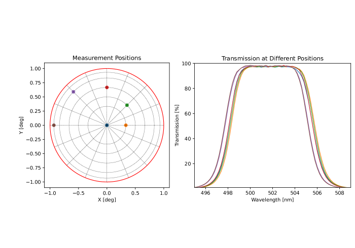
Figure 2: Left panel: The focal plane of DECam is shown as a red circle. Of the 49 positions at which the measurements were made, we only show the $N501$ filter transmission at the six positions indicated by the colored circles. Variations in the transmission curve are primarily a function of distance from the center. Right panel: While the transmission curve shifts blueward by a few angstroms near the edge of the field, it remains relatively constant over the bulk of the DECam focal plane. The behavior of $N419$ and $N673$ filters is similar to that shown in this figure.

The ODIN filters are designed for dual use, i.e., to promote both high-redshift and Galactic science. At zero velocity, the filter transmission at 4959 Å and 5007 Å is 10% and 99%, respectively. At $\Delta v=\pm 500$ km s^-1, the transmission changes to 5% (25%) and 97% (99%). Similarly, The $N673$ filter samples [S ii] emission at $|v|\leq 500$ km s^-1 at a nearly constant transmission.

A combination of $N673$ and $N501$ can identify [O iii] emitters at $z=0.34$ masquerading as $N673$-detected LAEs (N. Firestone et al. in preparation). For $N501$-detected LAEs at $z=3.1$, $N673$ samples He ii1640 emission to constrain their average stellar population properties via stacking analysis. For $N673$-detected LAEs at $z=4.5$, Lyman continuum radiation that leaks out can be detected in the $N501$ filter.

All three filters are circular in shape with a diameter of 620 mm and are designed to have a transmission curve as close as possible to a top hat in shape. The post-production lab measurements were made in a parallel beam with 5^∘ angle of incidence at the Asahi Spectra Ltd. facility on 49 points distributed along five concentric circles across the focal plane to characterize the variation of transmission. The expected transmission at normal incidence (f/3.6) is then computed based on these measurements. In Figure 2, we show the results at five different angular distances from the field center. As one moves farther away from the center of DECam’s 1.1^∘ circular field, the central wavelength tends to shift blueward, and the transmission increasingly deviates from being top-hat in shape.

The change in filter transmission as a function of field position is expected to have a negligible impact on our science goals. As we discuss in Section 4.1, the dither patterns for most ODIN fields are designed to minimize transmission variations by observing the same objects at many locations within the focal plane. Doing so ensures that, throughout a given field, the effective transmission is as close as possible to a weighted average of the curves shown in Figure 2. Upon observational validation of these fluctuations, it may be possible to utilize the transmission variation to perform a single-filter ‘tomography’ and determine a more precise redshift of bright LAEs (Zabl et al., 2016).

Table 1: Filter Summary

Filter	$\lambda_{C}$	$\lambda_{l}^{\ast}$	$\lambda_{u}^{\ast}$	FWHM	$z_{C}$	$\Delta z$
	[nm]	[nm]	[nm]	[nm]
$N419$	419.3	415.5	423.0	7.4	2.449	0.061
$N501$	501.4	497.6	505.2	7.2	3.124	0.059
$N673$	675.0	670.0	680.0	9.8	4.553	0.081

^∗$\lambda_{l}$ and $\lambda_{u}$ give the endpoints of each filter’s full width at half maximum (FWHM). $z_{C}$ and $\Delta z$ represent the central wavelength and the FWHM of each filter in redshift space, respectively.

3.2 ODIN Survey Fields

Table 2: Summary of ODIN Fields and Available Data

Field	Field Center	Area	Pointing Pattern	Notable Facts
	(J2000)	[deg2]
ELAIS-S1	9.45∘, $-44.00^{\circ}$	10	Two Rings	DDF
SHELA∗	$20.5^{\circ}$, $0.00^{\circ}$	24	Spiral	HETDEX, DESI access
XMM-LSS	$35.71^{\circ}$, $-4.75^{\circ}$	10	Two Rings	DDF, SSP, DESI access
CDF-S	$53.13^{\circ}$, $-28.10^{\circ}$	10	Two Rings	DDF, EDF
EDF-Sa	$58.90^{\circ}$, $-49.32^{\circ}$	10	Two Rings	EDF, SPHEREx DF
EDF-Sb	$63.60^{\circ}$, $-47.60^{\circ}$	10	Two Rings	EDF, SPHEREx DF
E-COSMOS	$150.10^{\circ}$, $2.18^{\circ}$	10	Two Rings	DDF, SSP, DESI access
Deep2-3	$352.1^{\circ}$, $-0.28^{\circ}$	7	Spiral	SSP, DESI access
Total	-	91
Survey	BB Filters		$5\sigma$ Point Source Sensitivity
SSP Deep†	$ugrizy$	-	27.1, 27.5, 27.1, 26.8, 26.3, 25.3
LSST DDF Y1	$ugrizy$	-	26.7, 27.9, 28.1, 27.4, 26.6, 25.3
LSST DDF Y10	$ugrizy$	-	28.0, 29.2, 29.4, 28.7, 27.9, 26.6
LSST Y3	$ugrizy$	-	25.6, 26.8, 27.0, 26.3, 25.5, 24.2
LSST Y10	$ugrizy$	-	26.3, 27.5, 27.7, 27.0, 26.2, 24.9

^†SSP Deep field sensitivities include those of the Subaru HSC data and of the CLAUDS $u$-band data from CFHT MegaCam (Sawicki et al., 2019). ^∗For SHELA, we give the RA range instead of the pointing center. DDF: LSST Deep Drilling Field (https://www.lsst.org/scientists/survey-design/ddf); SSP: Hyper SuprimeCam Subaru Strategic Plan (https://hsc.mtk.nao.ac.jp/ssp/survey); EDF: Euclid Deep Field (https://www.cosmos.esa.int/web/euclid/euclid-survey); HETDEX: the Hobby-Eberly Telescope Dark Energy eXperiment (https://hetdex.org); SPHEREx (https://spherex.caltech.edu/)

The choice of ODIN fields is based primarily on the maximum depth of existing or future broad-band imaging data, and in several cases, on the availability of spectroscopy. The seven ODIN fields include three of the Subaru Strategic Program deep fields, all five LSST Deep Drilling Fields (DDFs), two Euclid Deep Fields, and two fields with (nearly) full coverage of spectroscopic coverage from the Hobby-Eberly Telescope Dark Energy eXperiment (HETDEX). Together, these datasets will enable a wide range of scientific investigations on the properties of LAEs, the utility of LAEs as tracers of the large-scale structure, and identification of protoclusters and their signposts (Section 2). The complete list of the ODIN survey fields and their characteristics are presented in Table 2 and the layout of each field is summarized in Figure 3.

Within a year after the LSST begins, five of the seven ODIN fields will have the deepest wide-field optical data available (Table 2), surpassing the current depths of the SSP Deep fields. Three of the SSP deep fields are also ODIN fields, namely E-COSMOS, XMM-LSS, and Deep2-3, which are the priority fields for ODIN as they enable scientific investigations before the LSST begins. SHELA is one of the two fields being observed with a near 1:1 fill factor by the integral field spectrographs of HETDEX. Although SHELA is not part of any deep field imaging surveys, ODIN has been steadily improving on the BB depths in the area that offers continuous IRAC coverage.

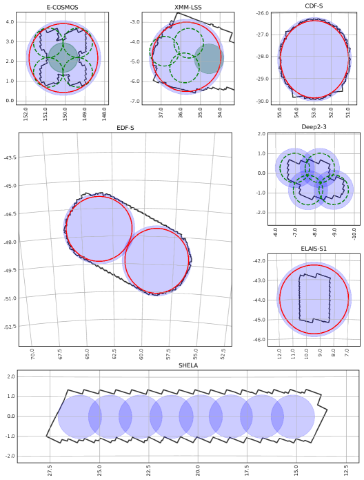
Figure 3: The layout of the seven ODIN fields. Blue shades indicate the area covered by ODIN at $\geq 70$% of the target depths. Red circles mark the LSST field of view. Green solid (dashed) circles denote the SSP ultradeep (deep) regions. All seven fields will receive LSST coverage. The existing Spitzer IRAC coverage is outlined in grey.

3.3 Survey parameters and expectations

The ODIN survey parameters are optimized for the detection of protoclusters as LAE overdensities. The ability to detect protoclusters as medium-scale enhancements above the average field depends on a combination of two factors. First, a high surface LAE density, $\Sigma_{\rm LAE}$, improves the significance of protocluster detection by lowering the Poisson fluctuations associated with galaxy counts. Second, a smaller line-of-sight thickness ($d_{\rm los}$) minimizes the projection effects that typically suppress, but sometimes enhance, measured overdensities. To this end, the detection efficiency parameter $p_{p}\equiv\Sigma_{\rm LAE}/d_{\rm los}$ is kept relatively constant at all three ODIN redshifts. However, the DECam Exposure Time Calculator (ETC) suggested that achieving the same $p_{p}$ level for $N673$ requires prohibitively large integration times ($\approx$ 50% more than $N419$ and $N501$ time combined). We therefore choose a slightly lower $p_{p}$ value to set the nominal depth for $N673$ observations.

While $d_{\rm los}$ is tied to the width of the filter transmission, the mean LAE surface density, $\Sigma_{\rm LAE}$, depends on the imaging depth. Because the broad-band data typically extend $\gtrsim$1 mag deeper than our narrow-band observations, $\Sigma_{\rm LAE}$ is primarily determined by the seeing and our narrow-band filter exposure times. We estimate the LAE surface density at a fixed NB depth using field Ly$\alpha$ LFs (Gronwall et al., 2007; Ouchi et al., 2008; Ciardullo et al., 2012; Sobral et al., 2018) interpolated to the redshift corresponding to each narrow-band filter’s central wavelength. In this estimate, we assume that the Ly$\alpha$ luminosity dominates the narrow-band flux density.

Table 3: Expectations for the ODIN survey

	$N419$	$N501$	$N673$	Total
Redshift	$2.45\pm 0.03$	$3.12\pm 0.03$	$4.55\pm 0.04$	-
Exp. Time [hr]	6.0	5.0	9.0	-
$5\sigma$ depth† [mag]	25.5	25.7	25.9	-
$5\sigma$ Line Flux [cgs∗]	$3.1\times 10^{-17}$	$1.8\times 10^{-17}$	$1.1\times 10^{-17}$	-
SB limit [cgs∗]	$3.5\times 10^{-18}$	$2.1\times 10^{-18}$	$1.2\times 10^{-18}$	-
Line-of-sight thickness [cMpc]	76.0	57.0	50.6	-
Cosmic Volume [cMpc3]	$7.43\times 10^{7}$	$7.04\times 10^{7}$	$8.50\times 10^{7}$	$2.30\times 10^{8}$
LAE density [arcmin-2]	$0.19$	$0.17$	$0.10$	$0.46$
Protocluster selection efficiency, $p_{p}$	$1.1\times 10^{-3}$	$1.3\times 10^{-3}$	$0.8\times 10^{-3}$	-
# of LAEs	60,000	50,000	30,000	140,000
# of protoclusters‡	14 (184)	13 (175)	16 (211)	42 (570)
# of LABs	268–1874	254–1775	308–2154	$\approx$800–5800

^†The limiting magnitudes are computed within 2″ diameter apertures assuming $1\farcs 2$, with seeing (and aperture) scaled with wavelength as predicted in the DECam ETC. We have assumed an average sky brightness corresponding to 0, 3, and 3 days from new moon for $N419$, $N501$, and $N673$, respectively.
^∗Line fluxes and surface brightness limits are given in units of erg s^-1 cm^-2 and erg s^-1 cm^-2 arcsec^-2.
^‡The number of Coma (Virgo) analogs expected within the survey volume.

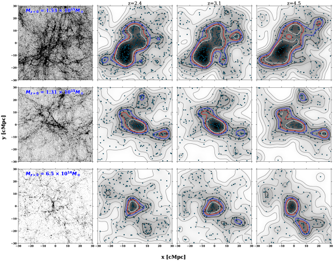
Figure 4: On the leftmost column, we show the dark matter distribution at $z=3$ around three present-day cosmic structures identified in the IllustrisTNG TNG300 simulation. In all cases, the line-of-sight thickness is 60 cMpc, roughly matched to the ODIN survey. The present-day masses are also indicated. Of the halos hosting galaxies with stellar mass $M_{\rm star}\geq 10^{9}M_{\odot}$, we randomly assign a subset as ‘LAEs’ to match the expected field LAE surface density at $z=2.4$, 3.1, and 4.5. The mass threshold is chosen to reproduce the observed LAE clustering strengths. The second, third, and fourth columns show the positions of these mock LAEs together with the Gaussian-kernel-smoothed density maps. The white, red, blue, and black lines denote $5\sigma$, $4\sigma$, $3\sigma$, and $2\sigma$ iso-surface-density contours, respectively. These images build clear expectations of how LAEs can trace massive cosmic structures at high redshift.

In Table 3, we list the nominal depths of our narrow-band data and the corresponding Ly$\alpha$ flux and the surface brightness limits. The expected LAE surface density and number of LAEs are also summarized. We also list the comoving line-of-sight thickness, the comoving cosmic volume, and the protocluster detection efficiency ($p_{p}$). In order to calculate the cosmic volume, we assume the full survey area of 91 deg². The expected number of protoclusters for each redshift slice is estimated based on this volume and the comoving number densities of clusters. As for the number densities of Coma- and Virgo-sized clusters (present-day masses of $\geq 10^{15}h^{-1}M_{\odot}$ and $(3-10)\times 10^{14}h^{-1}M_{\odot}$, respectively), we assume $1.84\times 10^{-7}$ and $2.48\times 10^{-6}$ cMpc^-3, respectively. These numbers are taken from the Millennium simulations-based (Springel et al., 2005) values computed by Chiang et al. (2013). The adopted cosmology for the simulation is only slightly different from ours and we do not make any additional corrections. The uncertainty due to Poisson shot noise and cosmic variances are expected to be larger than the changes from different cosmologies, particularly for the Coma progenitors.

As for the expected number of LABs, we assume a constant density across all redshifts. The number density estimate for bright and extended LABs ($L_{{\rm Ly}\alpha}\gtrsim 1.5\times 10^{43}$ erg s^-1, $A_{\rm iso}\geq 16$ arcsec²: Yang et al., 2010) is $1.0^{+1.8}_{-0.6}\times 10^{-5}$ cMpc^-3 adopting a cosmology with $\Omega=0.3$, $\Omega_{\Lambda}=0.7$, and $h=0.7$. The uncertainties reflect strong field-to-field variations as well as the uncertainties originating from shot noise for a small-area (1.2 deg²) survey. The values listed in Table 3 are corrected for the difference in cosmology which is at a $\approx$10% level. Recently, from the ODIN COSMOS/$N501$ data, Ramakrishnan et al. (2023) reported 129 LABs over a $\approx$9 deg² region, forecasting that the total number of LABs may be closer to the upper limit in the table. More stringent limits will be placed by combining the LAB samples in multiple fields (B.H. Moon et al., in preparation).

In Figure 4, we illustrate how massive structures may appear at the nominal $p_{p}$ range adopted by ODIN. Using the IllustrisTNG simulation suite (Weinberger et al., 2017), we first choose three massive structures. In terms of $M_{z=0}$, the total mass at $z=0$, they are ranked #1, #2, and #7, respectively. The dark matter distribution of these structures at $z=3$ is shown in the left panels. To match the survey parameters, we create a (60 cMpc)³ volume centered on the progenitor of each cluster at $z=3$. Adopting a minimum stellar mass of $M_{\rm star}=10^{9}~{}M_{\odot}$ to match the LAE clustering measurements from the literature (Gawiser et al., 2007; Kovač et al., 2007; Guaita et al., 2010; Kusakabe et al., 2018), we randomly select a subset of halos above the threshold that matches the ODIN surface densities (Table 3). The surface density map is then created by smoothing the ‘LAE’ distribution with a fixed kernel. We choose a two-dimensional Gaussian kernel with a full-width-at-half-maximum of $5\farcm 2$ (10 cMpc at $z=3$), comparable to the expected size of a protocluster. We note that, as a simple demonstration, we use the $z=3$ matter distribution in these structures to simulate the LAE maps at all three ODIN redshifts by simply matching the respective LAE surface densities.

Figure 4 demonstrates that ODIN is expected to detect Virgo- or Coma progenitors with ease provided that LAEs represent an unbiased tracer of low-mass halos. While we chose to use a random subset of halos as mock LAEs, more realistic modelings of LAEs following the recipes of Weinberger et al. (2019) or Mason et al. (2018) do not meaningfully alter the result (Lee et al., 2023, M. Andrews et al., in prep, S. Im et al., in prep). However, reality may be more complicated. Radiative transfer effects could cause LAEs to avoid the regions of highest density (e.g., see Momose et al., 2021; Huang et al., 2022). Additionally, as galaxies grow more massive, star formation activity is expected to ramp up and produce more interstellar dust, lowering their likelihood of being classified as LAEs (e.g., Weiss et al., 2021). These considerations suggest that the densest and most evolved regions may not be represented as the highest LAE overdensities. More observational evidence is needed to firmly establish the level of this potential bias.

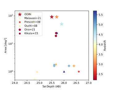
Figure 5: Comparison of the imaging depth and area coverage of recent surveys with ODIN (stars). All data are color-coded by redshift. Diamonds and circles represent the combined SILVERRUSH and CHORUS surveys (Ono et al., 2021; Kikuta et al., 2023). Earlier surveys with Subaru/SuprimeCam (Prescott et al., 2008; Ouchi et al., 2008, triangles and pentagon, respectively), Mayall/Mosaic (Malavasi et al., 2021, cross) are also listed.

In Figure 5, we show the areal coverage vs. depths of existing narrow-band $z$=2–5 Ly$\alpha$ surveys along with the ODIN survey. These studies include the combined results from the SILVERRUSH and CHORUS conducted with Subaru/HSC (Ono et al., 2021; Kikuta et al., 2023) as well as several earlier measurements with Subaru/SuprimeCam (Ouchi et al., 2008; Prescott et al., 2008) and Mayall/Mosaic3 (Malavasi et al., 2021).

4 Observations and Data Reduction

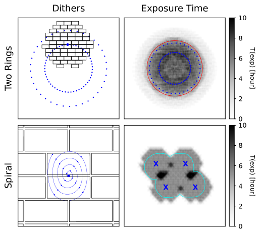
Figure 6: Two dither patterns used for the ODIN survey. Top left: Blue points mark the center position of each DECam pointing in the two-ring dither pattern. The radius of the inner and the outer ring is 1.0^∘ and 1.6^∘, respectively. The individual CCDs of DECam are shown in black. Top right: The resultant exposure map for $N419$ together with the pointing centers (blue points) and the LSST field-of-view (red circle). Bottom left: The spiral dither positions are overlaid on the center of the DECam focal plane, with individual CCDs shown in black. Small dithers along the spiral create an X-shaped set of pointings that enable uniform coverage by minimizing the overlap between chip gaps. Bottom right: The exposure map for $N419$ of the Deep2-3 field employs the spiral dither pattern of four overlapping fields. The pointing centers are shown in blue. The broad-band coverage from SSP is shown in cyan.

4.1 Dither patterns

DECam images a circular region of 2.1^∘ in diameter. In comparison, the LSST field-of-view (FOV) is 3.5^∘ in diameter. To achieve a reasonable level of uniformity across the five LSST DDFs using DECam, we designed a two-ring dither scheme as illustrated in the top left panel of Figure 6. DECam pointings are positioned along two concentric rings with radii 1.0^∘ and 1.6^∘ from the field center. The number of visits in each ring is determined based on the 1200 s exposure time per frame and the effective exposure time per pixel needed to reach the target depths as discussed in Section 4.2. The radii and total exposure time ratio of the rings are calibrated to minimize the variation of the depths in the radial direction by controlling the degree of overlap between the inner- and outer-ring exposures.

In the top right panel of Figure 6, we show the nominal exposure time map for the $N419$ observations in COSMOS. The final map is similar to this figure except for the presence of satellite trails. Each sky location within the LSST Deep Drilling Field gets observed by at least 10 pointings, naturally filling in chip gaps to yield locally uniform depth. The angular spacing between adjacent pointings in a given ring is smaller for the $N501$ and $N673$ observations because the exposure time per pixel is higher, but adheres to the same principle. The exposure maps of all DDF fields in all filters are expected to be similar to that shown in the figure.

In a given ring, we randomly shuffle the order in which pointings are observed to ensure uniformity in seeing across the field. We typically complete the inner ring pointings before starting the outer ring to enable early science. For the EDF-S, which is composed of two slightly overlapping LSST pointings, we randomly select pointings from rings in both EDFS-a and EDFS-b, as the CTIO 4m slew time from one to the other is never much larger than the DECam readout time.

For the fields that are not DDFs, namely, SHELA and Deep2-3, we take a different approach. For SHELA, we match the NB coverage as closely as possible to the existing BB data (Wold et al., 2019). The coverage is comprised of eight DECam pointings that follow a spiral pattern with small dithers to fill gaps, as shown in Figure 3. On the other hand, Deep2-3 is defined via four overlapping HSC pointings. In both SHELA and Deep2-3, we employ a spiral dither pattern. As illustrated in the bottom left panel of Figure 6, dither positions move away from the pointing center along a spiral by a small offset each time such that chip gaps along the RA and Dec axes never repeat, yielding an X-shaped pattern designed to fill the CCD gaps and to cover the BB regions with uniform coverage. In all narrow-band filters, we use the identical pattern repeating it as many times as needed to achieve the target depth.

4.2 ODIN data acquisition and reduction

The ODIN survey began its observations in February 2021. At the time of this article, the survey is $\approx$50% complete. A comprehensive summary of the LAE selection will be given elsewhere (N. Firestone et al., in preparation), and here we focus on the general practice adopted for our observations and data processing.

ODIN observations of all filters use an exposure time of 1200 sec, which is motivated by two considerations: the low sky background expected in narrow-band filters requires that our exposure times be long enough to ensure that the 7 e^- read noise of the DECam CCDs is not a dominant factor. According to the DECam exposure time calculator, in a 1200 sec exposure in $N419$, $N501$, and $N673$, the fraction of readout noise is $\approx$30, 13, and 4% of the sky background noise measured in a 2″ diameter circular aperture at new moon. A countervailing need is to avoid filling too much of the detector with cosmic rays, which, given the thick CCDs on DECam, can be highly extended and morphologically complex. This drives us to set a maximum exposure time of 1200s.

During our observations, we utilize the copilot software (Burleigh et al., 2020), a tool developed for DECam to monitor observing conditions and image weight. Using the Pan-STARRS-1 photometric catalog (Schlafly et al., 2012), copilot measures seeing, transparency ($T$), and sky brightness ($B$). Based on these data, we compute relative image weights, $w$, as:

$$w\propto\frac{T^{2}~{}{\rm{\tt exptime}}^{2}}{B{\rm~{}{\tt seeing}}^{2}}$$ (1)

The weight is normalized by values expected in a nominal dark sky condition. For ($N419$, $N501$,$N673$) a weight of unity would be achieved in a 1200 sec exposure with $T=1$, seeing of (1.2,1.1,1.0)″ and a background level of (50,100,200) ADU per pixel. The primary goal is to ensure that each designated pointing receives a combined weight of $\approx$1 by the completion of our observations. In practice, this means that the same pointing can be revisited to add more depth until the combined weight is similar to the original specification. The weighting scheme given in Equation 1 can accommodate shorter-exposure frames as long as readout noise remains sub-dominant.

We process and stack the ODIN data using the DECam Community Pipeline (CP: Valdes et al., 2014; Valdes, 2021) as follows. Each DECam exposure consisting of data from the 60 calibrateable CCDs is flat-fielded separately by dome flats, star flats, and dark sky illumination flats. Dark sky illumination flats are created by coadding unregistered stacks of exposures. Dome flats are produced by stacking sequences of 11 exposures taken each night; star flats are made from widely dithered exposures of a star field using the algorithm of Bernstein et al. (2017).

For each CCD, the background is measured by the modes of pixel values in small blocks with sources masked. Blocks with an insufficient number of background pixels are replaced by interpolation from nearby blocks. A spline surface is fit to the modes. In fields with prominent reflections from very bright stars, the modes are used directly to best handle the fine structure of the ghosts. The background is subtracted while maintaining the mean. The block size chosen to measure the background is sufficiently large to ensure that it does not introduce any photometric bias for extragalactic sources; however, since the size is smaller than the region affected by bright stars, the procedure can lead to over-subtraction of the faint halos.

The CP provides a data quality flag for every pixel for every exposure. The flags, in order of precedence, are known bad CCD pixels, saturated or bleed trail pixels, and cosmic ray and streak identifications. The last analysis is done on individual exposures but multiple ODIN exposures allow further identification via transient signals. In addition, the ODIN team produces satellite trail masks for affected exposures which are combined with the CP data quality masks. The pixels flagged in the master quality mask are excluded from consideration when coadding all the exposures to create the deep image stacks.

An astrometric solution is derived for each CCD by matching stars to Gaia-EDR3 (Gaia Collaboration et al., 2021). While the higher order distortions are predetermined and fixed, the low order terms are updated using the astrometric solver SCAMP (Bertin, 2006) with continuity constraints between CCDs. The root-mean-square of a plate solution is typically a few hundredths of an arcsecond. We reproject the exposures to a standard tangent plane sampling at the pixel scale of $0\farcs 27$/pix using sinc interpolation. A fixed tangent point is used for all the exposures in a given field with the exception of the two largest ODIN fields which are more than 10^∘ across. For EDF-S and SHELA, two and four separate tangent points are used.

Individual exposures are matched to the Pan-STARRS-1 photometric catalog (Schlafly et al., 2012) to determine a zeropoint (magzero) and a photometric depth in magnitude (depth). The latter is computed as:

$${\tt depth}={\tt magzero}-2.5\log\left(5\sigma\sqrt{\pi r^{2}_{\rm op}}\right)$$ (2)

where $\sigma$ is the pixelwise sky noise and $r_{\rm op}$ represents the size of an optimal aperture (for a pure Gaussian seeing) whose diameter is 1.35 times the measured seeing FWHM. The magzero parameter combines sky transparency and exposure time for a given frame while depth represents the $5\sigma$ uncertainty. The depth parameter is then converted to linear relative counts and squared to form a normalized relative weight for each frame. All exposures are coadded as a weighted mean with statistical rejection (constrained sigma clipping) of outliers to remove the large number of cosmic rays accumulated in our long exposures.

In Figure 7, we show the full-depth mosaic of CDF-S in $N501$ overlaid with the LSST field-of-view (yellow circle) and the size of the Moon. Similar to the SSP data release, the ODIN stack is split into multiple ‘tracts’, each $1.7^{\circ}\times 1.7^{\circ}$ in size with an overlap of 1′ for the ease of data handling. The only exception to this convention is SHELA, for which we create four separate stacks each of which contains two adjacent DECam pointings.

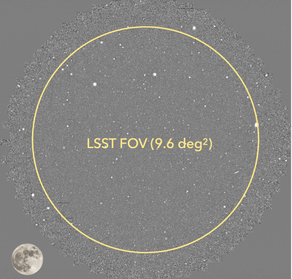
Figure 7: The final mosaic of CDF-S in $N501$ is shown. The yellow circle marks the position and area coverage of the planned LSST observations of CDF-S in $ugrizy$ at the DDF depths indicated in Table 2. The to-scale size of the Moon is shown at the bottom left corner.

5 External Data

5.1 Broad-band optical data

The detection of high-redshift LAEs requires that the ODIN narrow-band data be compared existing broad-band frames. For the Deep2-3, E-COSMOS, and XMM-LSS fields, these data come from the HSC SSP program (Aihara et al., 2018). Specifically, we use the publicly available frames from the third data release (Aihara et al., 2022). Similar to that described in Section 4.2, we reproject the data using the common tangent point at the pixel scale of $0\farcs 27$/pix.

In the SHELA field, we use the archival DECam data taken as part of several NOIRLab programs. As described in Wold et al. (2019), the existing observations are composed of eight overlapping DECam pointings. We reprocess the data using the DECam CP and find that the depths vary significantly across the field. Since Fall 2021, ODIN has been conducting additional DECam imaging with the primary goal of homogenizing the sensitivity of broad-band data with the top priority on the $gr$ bands to enable a uniform selection of LAEs.

In the remaining three fields (EDF-Sab, ELAIS-S1, and CDF-S), the availability of the BB data across the $\sim 10$ deg² field is currently limited. A subsection of CDF-S was observed repeatedly as one of the Dark Energy Survey deep fields (Hartley et al., 2022) designed to detect supernovae. While the approximate depths of these data are listed in Table 2, the sensitivity will be easily surpassed in 2026 by Rubin with uniform coverage within the ODIN fields. These considerations have been taken into account in setting the observational priorities.

5.2 Spitzer IRAC data

All seven ODIN fields have existing Spitzer IRAC images which cover a substantial fraction of the survey area at depths that are useful for selecting massive galaxies in the ODIN redshift range. These datasets will enable statistical association of massive galaxies with cosmic structures and/or Ly$\alpha$ blobs and elucidate the early formation histories of massive cluster ellipticals. The IRAC coverage of the ODIN fields is indicated by grey lines in Figure 3. Here, we briefly summarize the publicly available data.

The COSMIC DAWN survey (Euclid Collaboration et al., 2022) obtained IRAC imaging of three Euclid Deep Fields. In all cases, we quote the $5\sigma$ detection limit, which is $\approx$0.5 $\mu$Jy for EDF-N and CDF-S (i.e., the Euclid Deep Field Fornax) and $\approx$1.0 $\mu$Jy for EDF-S. Additionally, Cosmic Dawn re-reduced all existing IRAC datasets in other Euclid calibration fields including XMM-LSS and COSMOS (both at $\approx$1.0 $\mu$Jy) in a consistent manner. Smaller subsections of COSMOS, XMM-LSS, and CDF-S have also been imaged to varying depths by other programs. For a summary of the depths and areal coverage, we refer interested readers to Euclid Collaboration et al. (2022).

ELAIS-S1 and Deep2-3 are covered by the Spitzer Extragalactic Representative Volume Survey (SERVS; Mauduit et al., 2012), and the Spitzer coverage of HSC-Deep with IRAC for Z (SHIRAZ; Annunziatella et al., 2023) survey, respectively, at a comparable depth of $\approx$1 $\mu$Jy. A larger section of ELAIS-S1 is imaged at a shallower depth ($\approx$3 $\mu$Jy) by the Spitzer Wide-area InfraRed Extragalactic survey (SWIRE; Lonsdale et al., 2003). Finally, the imaging of the SHELA was performed by the Spitzer-HETDEX Exploratory Large Area survey (SHELA: Papovich et al., 2016) at the shallowest depth (5.5 $\mu$Jy), which corresponds to a star-forming galaxy of moderate dust reddening, $E(B-V)=0.25$ and stellar mass of $\approx 10^{10.2}M_{\odot}$ at $z=2.5$.

5.3 Spectroscopy

Multiple ongoing spectroscopic programs are targeting ODIN-selected galaxies with DESI, Gemini GMOS, Keck DEIMOS, and the Prime Focus Imaging Spectrograph on the South African Large Telescope. These data have been highly successful in validating LAE selection, measuring the spatial structure of several protoclusters, and spectroscopically confirming more than 40 Ly$\alpha$ blobs. Presently, the number of ODIN LAEs with spectroscopic follow-up is $\approx$8,000, 3,000, and 800 at $z=2.4$, 3.1, and 4.5, respectively. The results from these programs will be presented in forthcoming papers.

6 Ancillary Science

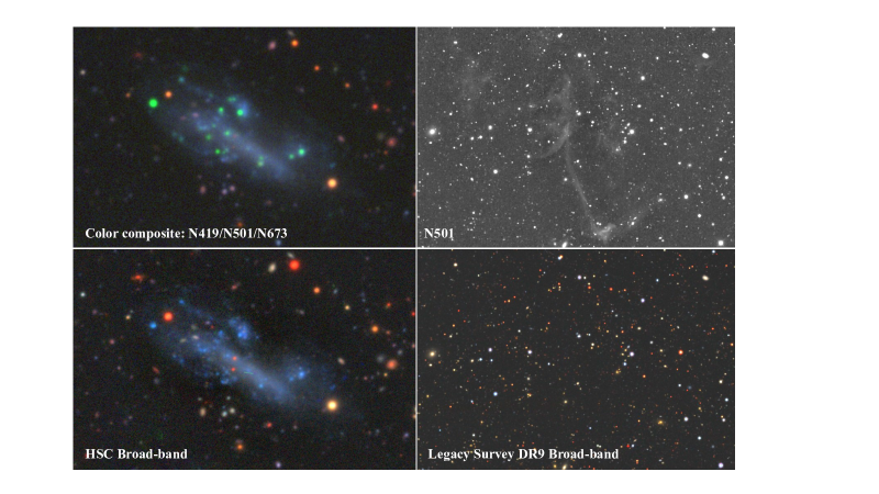
Figure 8: Left panels: A color-composite image of a nearby star-forming galaxy is displayed using the ODIN NB filters (top) and the HSC broad-band filters (bottom). Star-forming knots are clearly delineated in the former in green as $N501$ samples O iii nebular emission. Right panels: Extended large-scale features, visible in the $N501$ image (top), likely trace shocked, [O iii]-emitting gas associated with a planetary nebula, NGC 1360 located outside the ODIN field.

The deep NB data taken as part of ODIN can be used for a number of programs. These data can be visualized from the ODIN Legacy Viewer where users can browse each stacked ODIN narrow-band image as well as a color composite frame that combines the ODIN NB data together.

The left panels of Figure 8 show a nearby star-forming galaxy located at $(\alpha,\delta)=(149.620^{\circ},+1.694^{\circ})$. The colors are computed from ODIN data (top) and HSC broad-band images (bottom). Star-forming knots with strong [O iii] emission are clearly delineated as green features in the top panel. The right panels show a small section in CDF-S centered on $(\alpha,\delta)=(53.164^{\circ},-26.219^{\circ})$ observed in $N501$ (top right) with Legacy Survey DR9 broad-band data (bottom right). The complex and very extended [O iii] emission feature likely originates from shocked gas associated with NGC 1360, a planetary nebula located at $(\alpha,\delta)=(53.311^{\circ},-25.870^{\circ})$, $\approx$20′ northeast and outside the ODIN field. In the legacy viewer, the gas is captured in the broad-band data but only very close to NGC 1360. The sensitivity of the $N501$ and $N673$ data afforded by ODIN provides a unique opportunity to explore faint gaseous components of our Galaxy and star-forming regions of the nearby universe (e.g. Drechsler et al., 2023).

7 Summary

The ODIN collaboration is currently conducting a narrow-band survey with the largest area, covering $\approx 90$ deg² with three custom filters down to depths of 25.5–25.9 AB. By sampling redshifted Ly$\alpha$ emission at $z=2.4$, 3.1, and 4.5 in narrow cosmic slices ($\approx 60$ cMpc in thickness) within a 0.25 cGpc³ volume, ODIN will enable robust measurements of the epochs’ large-scale structure by mapping out knots, groups, filaments, and cosmic voids within the underlying matter distribution using low-mass, Ly$\alpha$-emitting galaxies.

ODIN will discover hundreds of distant protoclusters and thousands of the largest and most luminous Ly$\alpha$ nebulae, allowing us to study the physical association of these two rare types of cosmic objects and their relationships to the surrounding LSS. Through measurements of the LAE luminosity functions, spectral energy distribution, and clustering, we will determine the physical properties of these objects and their association with dark matter halos and obtain quantitative measurements of how LSS influences galaxy formation. The models of expansion history will be explored through measurements across cosmic time.

With Rubin, Euclid, and Roman on the horizon, the ODIN fields will become the deepest fields rich with spectroscopic and imaging data. When combined with these data, the ODIN data will have a lasting legacy in advancing studies of not only galaxy evolution at high redshift but also the Galaxy and the nearby universe.

References

- Adelberger et al. (2005) Adelberger, K. L., Steidel, C. C., Pettini, M., et al. 2005, ApJ, 619, 697, doi: 10.1086/426580
- Aihara et al. (2018) Aihara, H., Arimoto, N., Armstrong, R., et al. 2018, PASJ, 70, S4, doi: 10.1093/pasj/psx066
- Aihara et al. (2022) Aihara, H., AlSayyad, Y., Ando, M., et al. 2022, PASJ, 74, 247, doi: 10.1093/pasj/psab122
- Annunziatella et al. (2023) Annunziatella, M., Sajina, A., Stefanon, M., et al. 2023, AJ, 166, 25, doi: 10.3847/1538-3881/acd773
- Appleby et al. (2021) Appleby, S., Park, C., Hong, S. E., et al. 2021, Astrophys. J., 907, 75, doi: 10.3847/1538-4357/abcebb
- Appleby et al. (2017) Appleby, S., Park, C., Hong, S. E., & Kim, J. 2017, Astrophys. J., 836, 45, doi: 10.3847/1538-4357/836/1/45
- Arrigoni Battaia et al. (2019) Arrigoni Battaia, F., Hennawi, J. F., Prochaska, J. X., et al. 2019, MNRAS, 482, 3162, doi: 10.1093/mnras/sty2827
- Baldry et al. (2006) Baldry, I. K., Balogh, M. L., Bower, R. G., et al. 2006, MNRAS, 373, 469, doi: 10.1111/j.1365-2966.2006.11081.x
- Bernstein et al. (2017) Bernstein, G. M., Abbott, T. M. C., Desai, S., et al. 2017, PASP, 129, 114502, doi: 10.1088/1538-3873/aa858e
- Bertin (2006) Bertin, E. 2006, in Astronomical Society of the Pacific Conference Series, Vol. 351, Astronomical Data Analysis Software and Systems XV, ed. C. Gabriel, C. Arviset, D. Ponz, & S. Enrique, 112
- Blakeslee et al. (2003) Blakeslee, J. P., Franx, M., Postman, M., et al. 2003, ApJ, 596, L143, doi: 10.1086/379234
- Bond et al. (1996) Bond, J. R., Kofman, L., & Pogosyan, D. 1996, Nature, 380, 603, doi: 10.1038/380603a0
- Borisova et al. (2016) Borisova, E., Cantalupo, S., Lilly, S. J., et al. 2016, ApJ, 831, 39, doi: 10.3847/0004-637X/831/1/39
- Bădescu et al. (2017) Bădescu, T., Yang, Y., Bertoldi, F., et al. 2017, ApJ, 845, 172, doi: 10.3847/1538-4357/aa8220
- Burleigh et al. (2020) Burleigh, K. J., Landriau, M., Dey, A., et al. 2020, AJ, 160, 61, doi: 10.3847/1538-3881/ab93b9
- Cantalupo et al. (2014) Cantalupo, S., Arrigoni-Battaia, F., Prochaska, J. X., Hennawi, J. F., & Madau, P. 2014, Nature, 506, 63, doi: 10.1038/nature12898
- Casey (2016) Casey, C. M. 2016, ApJ, 824, 36, doi: 10.3847/0004-637X/824/1/36
- Cen & Zheng (2013) Cen, R., & Zheng, Z. 2013, ApJ, 775, 112, doi: 10.1088/0004-637X/775/2/112
- Chang et al. (2023) Chang, S.-J., Yang, Y., Seon, K.-I., Zabludoff, A., & Lee, H.-W. 2023, ApJ, 945, 100, doi: 10.3847/1538-4357/acac98
- Chiang et al. (2013) Chiang, Y.-K., Overzier, R., & Gebhardt, K. 2013, ApJ, 779, 127, doi: 10.1088/0004-637X/779/2/127
- Chiang et al. (2014) —. 2014, ApJ, 782, L3, doi: 10.1088/2041-8205/782/1/L3
- Ciardullo et al. (2012) Ciardullo, R., Gronwall, C., Wolf, C., et al. 2012, ApJ, 744, 110, doi: 10.1088/0004-637X/744/2/110
- Cucciati et al. (2018) Cucciati, O., Lemaux, B. C., Zamorani, G., et al. 2018, A&A, 619, A49, doi: 10.1051/0004-6361/201833655
- Daddi et al. (2021) Daddi, E., Valentino, F., Rich, R. M., et al. 2021, A&A, 649, A78, doi: 10.1051/0004-6361/202038700
- Daddi et al. (2022) Daddi, E., Rich, R. M., Valentino, F., et al. 2022, ApJ, 926, L21, doi: 10.3847/2041-8213/ac531f
- Dey et al. (2016) Dey, A., Lee, K.-S., Reddy, N., et al. 2016, ApJ, 823, 11, doi: 10.3847/0004-637X/823/1/11
- Dey et al. (2005) Dey, A., Bian, C., Soifer, B. T., et al. 2005, ApJ, 629, 654, doi: 10.1086/430775
- Dong et al. (2023) Dong, F., Park, C., Hong, S. E., et al. 2023, Astrophys. J., 953, 98, doi: 10.3847/1538-4357/acd185
- Drechsler et al. (2023) Drechsler, M., Strottner, X., Sainty, Y., et al. 2023, Research Notes of the American Astronomical Society, 7, 1, doi: 10.3847/2515-5172/acaf7e
- Eisenhardt et al. (2008) Eisenhardt, P. R. M., Brodwin, M., Gonzalez, A. H., et al. 2008, ApJ, 684, 905, doi: 10.1086/590105
- Ellison et al. (2008) Ellison, S. L., Patton, D. R., Simard, L., & McConnachie, A. W. 2008, AJ, 135, 1877, doi: 10.1088/0004-6256/135/5/1877
- Erb et al. (2011) Erb, D. K., Bogosavljević, M., & Steidel, C. C. 2011, ApJ, 740, L31, doi: 10.1088/2041-8205/740/1/L31
- Euclid Collaboration et al. (2022) Euclid Collaboration, Moneti, A., McCracken, H. J., et al. 2022, A&A, 658, A126, doi: 10.1051/0004-6361/202142361
- Fardal et al. (2001) Fardal, M. A., Katz, N., Gardner, J. P., et al. 2001, ApJ, 562, 605, doi: 10.1086/323519
- Francis et al. (1996) Francis, P. J., Woodgate, B. E., Warren, S. J., et al. 1996, ApJ, 457, 490, doi: 10.1086/176747
- Gaia Collaboration et al. (2021) Gaia Collaboration, Brown, A. G. A., Vallenari, A., et al. 2021, A&A, 649, A1, doi: 10.1051/0004-6361/202039657
- Gawiser et al. (2006) Gawiser, E., van Dokkum, P. G., Gronwall, C., et al. 2006, ApJ, 642, L13, doi: 10.1086/504467
- Gawiser et al. (2007) Gawiser, E., Francke, H., Lai, K., et al. 2007, ApJ, 671, 278, doi: 10.1086/522955
- Giavalisco & Dickinson (2001) Giavalisco, M., & Dickinson, M. 2001, ApJ, 550, 177, doi: 10.1086/319715
- Gronwall et al. (2007) Gronwall, C., Ciardullo, R., Hickey, T., et al. 2007, ApJ, 667, 79, doi: 10.1086/520324
- Guaita et al. (2010) Guaita, L., Gawiser, E., Padilla, N., et al. 2010, ApJ, 714, 255, doi: 10.1088/0004-637X/714/1/255
- Guaita et al. (2011) Guaita, L., Acquaviva, V., Padilla, N., et al. 2011, ApJ, 733, 114, doi: 10.1088/0004-637X/733/2/114
- Haiman et al. (2000) Haiman, Z., Spaans, M., & Quataert, E. 2000, ApJ, 537, L5, doi: 10.1086/312754
- Hartley et al. (2022) Hartley, W. G., Choi, A., Amon, A., et al. 2022, MNRAS, 509, 3547, doi: 10.1093/mnras/stab3055
- Hu & McMahon (1996) Hu, E. M., & McMahon, R. G. 1996, Nature, 382, 231, doi: 10.1038/382231a0
- Huang et al. (2022) Huang, Y., Lee, K.-S., Cucciati, O., et al. 2022, ApJ, 941, 134, doi: 10.3847/1538-4357/ac9ea4
- Hwang et al. (2011) Hwang, H. S., Elbaz, D., Dickinson, M., et al. 2011, A&A, 535, A60, doi: 10.1051/0004-6361/201117476
- Inoue et al. (2020) Inoue, A. K., Yamanaka, S., Ouchi, M., et al. 2020, PASJ, 72, 101, doi: 10.1093/pasj/psaa100
- Kikuta et al. (2023) Kikuta, S., Ouchi, M., Shibuya, T., et al. 2023, arXiv e-prints, arXiv:2305.08921, doi: 10.48550/arXiv.2305.08921
- Kollmeier et al. (2010) Kollmeier, J. A., Zheng, Z., Davé, R., et al. 2010, ApJ, 708, 1048, doi: 10.1088/0004-637X/708/2/1048
- Kovač et al. (2007) Kovač, K., Somerville, R. S., Rhoads, J. E., Malhotra, S., & Wang, J. 2007, ArXiv:0706.0893, 706
- Kusakabe et al. (2018) Kusakabe, H., Shimasaku, K., Ouchi, M., et al. 2018, PASJ, 70, 4, doi: 10.1093/pasj/psx148
- Laursen & Sommer-Larsen (2007) Laursen, P., & Sommer-Larsen, J. 2007, ApJ, 657, L69, doi: 10.1086/513191
- Lee et al. (2021) Lee, J., Shin, J., Snaith, O. N., et al. 2021, The Astrophysical Journal, 908, 11, doi: 10.3847/1538-4357/abd08b
- Lee et al. (2023) Lee, J., Park, C., Kim, J., et al. 2023, arXiv e-prints, arXiv:2308.00571, doi: 10.48550/arXiv.2308.00571
- Lee et al. (2014) Lee, K.-S., Dey, A., Hong, S., et al. 2014, ApJ, 796, 126, doi: 10.1088/0004-637X/796/2/126
- Lee et al. (2006) Lee, K.-S., Giavalisco, M., Gnedin, O. Y., et al. 2006, ApJ, 642, 63, doi: 10.1086/500387
- Lemaux et al. (2022) Lemaux, B. C., Cucciati, O., Le Fèvre, O., et al. 2022, A&A, 662, A33, doi: 10.1051/0004-6361/202039346
- Lonsdale et al. (2003) Lonsdale, C. J., Smith, H. E., Rowan-Robinson, M., et al. 2003, PASP, 115, 897, doi: 10.1086/376850
- Madau & Dickinson (2014) Madau, P., & Dickinson, M. 2014, ARA&A, 52, 415, doi: 10.1146/annurev-astro-081811-125615
- Malavasi et al. (2021) Malavasi, N., Lee, K.-S., Dey, A., et al. 2021, ApJ, 921, 103, doi: 10.3847/1538-4357/ac1c6e
- Mancone et al. (2010) Mancone, C. L., Gonzalez, A. H., Brodwin, M., et al. 2010, ApJ, 720, 284, doi: 10.1088/0004-637X/720/1/284
- Mason et al. (2018) Mason, C. A., Treu, T., Dijkstra, M., et al. 2018, ApJ, 856, 2, doi: 10.3847/1538-4357/aab0a7
- Matsuda et al. (2004) Matsuda, Y., Yamada, T., Hayashino, T., et al. 2004, AJ, 128, 569, doi: 10.1086/422020
- Matsuda et al. (2011) —. 2011, MNRAS, 410, L13, doi: 10.1111/j.1745-3933.2010.00969.x
- Mauduit et al. (2012) Mauduit, J. C., Lacy, M., Farrah, D., et al. 2012, PASP, 124, 714, doi: 10.1086/666945
- Mei et al. (2006) Mei, S., Holden, B. P., Blakeslee, J. P., et al. 2006, ApJ, 644, 759, doi: 10.1086/503826
- Merlin et al. (2021) Merlin, E., Castellano, M., Santini, P., et al. 2021, A&A, 649, A22, doi: 10.1051/0004-6361/202140310
- Momose et al. (2021) Momose, R., Shimasaku, K., Kashikawa, N., et al. 2021, ApJ, 909, 117, doi: 10.3847/1538-4357/abd2af
- Muldrew et al. (2015) Muldrew, S. I., Hatch, N. A., & Cooke, E. A. 2015, MNRAS, 452, 2528, doi: 10.1093/mnras/stv1449
- Nayyeri et al. (2017) Nayyeri, H., Hemmati, S., Mobasher, B., et al. 2017, ApJS, 228, 7, doi: 10.3847/1538-4365/228/1/7
- Noeske et al. (2007) Noeske, K. G., Weiner, B. J., Faber, S. M., et al. 2007, ApJ, 660, L43, doi: 10.1086/517926
- Norberg et al. (2002) Norberg, P., Baugh, C. M., Hawkins, E., et al. 2002, MNRAS, 332, 827, doi: 10.1046/j.1365-8711.2002.05348.x
- Oke & Gunn (1983) Oke, J. B., & Gunn, J. E. 1983, ApJ, 266, 713, doi: 10.1086/160817
- Ono et al. (2021) Ono, Y., Itoh, R., Shibuya, T., et al. 2021, ApJ, 911, 78, doi: 10.3847/1538-4357/abea15
- Ouchi et al. (2020) Ouchi, M., Ono, Y., & Shibuya, T. 2020, ARA&A, 58, 617, doi: 10.1146/annurev-astro-032620-021859
- Ouchi et al. (2003) Ouchi, M., et al. 2003, ApJ, 582, 60, doi: 10.1086/344476
- Ouchi et al. (2008) Ouchi, M., Shimasaku, K., Akiyama, M., et al. 2008, ApJS, 176, 301, doi: 10.1086/527673
- Ouchi et al. (2010) Ouchi, M., Shimasaku, K., Furusawa, H., et al. 2010, ApJ, 723, 869, doi: 10.1088/0004-637X/723/1/869
- Ouchi et al. (2018) Ouchi, M., Harikane, Y., Shibuya, T., et al. 2018, PASJ, 70, S13, doi: 10.1093/pasj/psx074
- Overzier (2016) Overzier, R. A. 2016, A&A Rev., 24, 14, doi: 10.1007/s00159-016-0100-3
- Overzier et al. (2013) Overzier, R. A., Nesvadba, N. P. H., Dijkstra, M., et al. 2013, ApJ, 771, 89, doi: 10.1088/0004-637X/771/2/89
- Papovich et al. (2016) Papovich, C., Shipley, H. V., Mehrtens, N., et al. 2016, ApJS, 224, 28, doi: 10.3847/0067-0049/224/2/28
- Park & Kim (2010) Park, C., & Kim, Y.-R. 2010, Astrophys. J. Lett., 715, L185, doi: 10.1088/2041-8205/715/2/L185
- Park et al. (2022) Park, C., Lee, J., Kim, J., et al. 2022, The Astrophysical Journal, 937, 15, doi: 10.3847/1538-4357/ac85b5
- Park et al. (2019) Park, H., Park, C., Sabiu, C. G., et al. 2019, doi: 10.3847/1538-4357/ab2da1
- Partridge & Peebles (1967) Partridge, R. B., & Peebles, P. J. E. 1967, ApJ, 147, 868, doi: 10.1086/149079
- Peng et al. (2010) Peng, Y.-j., Lilly, S. J., Kovač, K., et al. 2010, ApJ, 721, 193, doi: 10.1088/0004-637X/721/1/193
- Planck Collaboration et al. (2015) Planck Collaboration, Aghanim, N., Altieri, B., et al. 2015, A&A, 582, A30, doi: 10.1051/0004-6361/201424790
- Prescott et al. (2008) Prescott, M. K. M., Kashikawa, N., Dey, A., & Matsuda, Y. 2008, ApJ, 678, L77, doi: 10.1086/588606
- Ramakrishnan et al. (2023) Ramakrishnan, V., Moon, B., Im, S. H., et al. 2023, ApJ, 951, 119, doi: 10.3847/1538-4357/acd341
- Reiprich & Böhringer (2002) Reiprich, T. H., & Böhringer, H. 2002, ApJ, 567, 716, doi: 10.1086/338753
- Saito et al. (2006) Saito, T., Shimasaku, K., Okamura, S., et al. 2006, ApJ, 648, 54, doi: 10.1086/505678
- Sawicki et al. (2019) Sawicki, M., Arnouts, S., Huang, J., et al. 2019, MNRAS, 489, 5202, doi: 10.1093/mnras/stz2522
- Schlafly et al. (2012) Schlafly, E. F., Finkbeiner, D. P., Jurić, M., et al. 2012, ApJ, 756, 158, doi: 10.1088/0004-637X/756/2/158
- Sheth et al. (2001) Sheth, R. K., Mo, H. J., & Tormen, G. 2001, MNRAS, 323, 1, doi: 10.1046/j.1365-8711.2001.04006.x
- Shi et al. (2019) Shi, K., Lee, K.-S., Dey, A., et al. 2019, ApJ, 871, 83, doi: 10.3847/1538-4357/aaf85d
- Sobral et al. (2018) Sobral, D., Santos, S., Matthee, J., et al. 2018, MNRAS, 476, 4725, doi: 10.1093/mnras/sty378
- Springel et al. (2005) Springel, V., White, S. D. M., Jenkins, A., et al. 2005, Nature, 435, 629, doi: 10.1038/nature03597
- Stanford et al. (1998) Stanford, S. A., Eisenhardt, P. R., & Dickinson, M. 1998, ApJ, 492, 461, doi: 10.1086/305050
- Steidel et al. (1999) Steidel, C. C., Adelberger, K. L., Giavalisco, M., Dickinson, M., & Pettini, M. 1999, ApJ, 519, 1, doi: 10.1086/307363
- Steidel et al. (2000) Steidel, C. C., Adelberger, K. L., Shapley, A. E., et al. 2000, 532, 170. http://adsabs.harvard.edu/cgi-bin/nph-bib_query?bibcode=2000ApJ...532..170S&db_key=AST
- Stevans et al. (2021) Stevans, M. L., Finkelstein, S. L., Kawinwanichakij, L., et al. 2021, ApJ, 921, 58, doi: 10.3847/1538-4357/ac0cf6
- Taniguchi & Shioya (2000) Taniguchi, Y., & Shioya, Y. 2000, ApJ, 532, L13, doi: 10.1086/312557
- Thomas et al. (2005) Thomas, D., Maraston, C., Bender, R., & Mendes de Oliveira, C. 2005, ApJ, 621, 673, doi: 10.1086/426932
- Topping et al. (2018) Topping, M. W., Shapley, A. E., Steidel, C. C., Naoz, S., & Primack, J. R. 2018, ApJ, 852, 134, doi: 10.3847/1538-4357/aa9f0f
- Toshikawa et al. (2018) Toshikawa, J., Uchiyama, H., Kashikawa, N., et al. 2018, PASJ, 70, S12, doi: 10.1093/pasj/psx102
- Umehata et al. (2019) Umehata, H., Fumagalli, M., Smail, I., et al. 2019, Science, 366, 97, doi: 10.1126/science.aaw5949
- Valdes (2021) Valdes, F. 2021, The DECam Community Pipeline Instrumental Signature Removal. https://legacy.noirlab.edu/noao/staff/fvaldes/Pipelines/Docs/PL206/
- Valdes et al. (2014) Valdes, F., Gruendl, R., & DES Project. 2014, in Astronomical Society of the Pacific Conference Series, Vol. 485, Astronomical Society of the Pacific Conference Series, ed. N. Manset & P. Forshay, 379
- van der Burg et al. (2020) van der Burg, R. F. J., Rudnick, G., Balogh, M. L., et al. 2020, A&A, 638, A112, doi: 10.1051/0004-6361/202037754
- Vargas et al. (2014) Vargas, C. J., Bish, H., Acquaviva, V., et al. 2014, ApJ, 783, 26, doi: 10.1088/0004-637X/783/1/26
- Weaver et al. (2021) Weaver, J. R., Kauffmann, O. B., Ilbert, O., et al. 2021, arXiv e-prints, arXiv:2110.13923. https://arxiv.org/abs/2110.13923
- Weinberger et al. (2019) Weinberger, L. H., Haehnelt, M. G., & Kulkarni, G. 2019, MNRAS, 485, 1350, doi: 10.1093/mnras/stz481
- Weinberger et al. (2017) Weinberger, R., Springel, V., Hernquist, L., et al. 2017, MNRAS, 465, 3291, doi: 10.1093/mnras/stw2944
- Weiss et al. (2021) Weiss, L. H., Bowman, W. P., Ciardullo, R., et al. 2021, ApJ, 912, 100, doi: 10.3847/1538-4357/abedb9
- Wold et al. (2019) Wold, I. G. B., Kawinwanichakij, L., Stevans, M. L., et al. 2019, ApJS, 240, 5, doi: 10.3847/1538-4365/aaee85
- Xue et al. (2017) Xue, R., Lee, K.-S., Dey, A., et al. 2017, ApJ, 837, 172, doi: 10.3847/1538-4357/837/2/172
- Yang et al. (2009) Yang, X., Mo, H. J., & van den Bosch, F. C. 2009, ApJ, 695, 900, doi: 10.1088/0004-637X/695/2/900
- Yang et al. (2014) Yang, Y., Walter, F., Decarli, R., et al. 2014, ApJ, 784, 171, doi: 10.1088/0004-637X/784/2/171
- Yang et al. (2010) Yang, Y., Zabludoff, A., Eisenstein, D., & Davé, R. 2010, ApJ, 719, 1654, doi: 10.1088/0004-637X/719/2/1654
- York et al. (2000) York, D. G., Adelman, J., Anderson, Jr., J. E., et al. 2000, AJ, 120, 1579
- Zabl et al. (2016) Zabl, J., Freudling, W., Møller, P., et al. 2016, A&A, 590, A66, doi: 10.1051/0004-6361/201526378