The three-quasi-particle scattering problem: asymptotic completeness for short-range systems

Abstract

We develop an approach to scattering theory for generalized $N$-body systems. In particular we consider a general class of three quasi-particle systems, for which we prove Asymptotic Completeness.

1 Introduction

In this note we study the scattering theory of a three-quasi-particle system. The system is described by the following equation:

$$\begin{cases}i\partial_{t}\psi(x,t)=(H_{0}+V(x))\psi(x,t)\\ \psi(x,0)=\psi_{0}(x)\in\mathcal{L}^{2}_{x}(\mathbb{R}^{9})\end{cases},\quad x=(x_{1},x_{2},x_{3})\in\mathbb{R}^{9}.$$ (1.1)

Here, we define:

• $x_{j}\in\mathbb{R}^{3}$(with $j=1,\cdots,3$) represents the position variable of the $j$th particle.

• $P_{j}:=-i\nabla_{x_{j}}$ represents the wave number operator of the $j$th particle, often referred to as the quasi-momentum.

• $H_{0}=\sum\limits_{j=1}^{3}\omega_{j}(P_{j})$, where $\omega_{j}:\mathbb{R}^{3}\to\mathbb{R},\eta\mapsto\omega_{j}(\eta)$, denotes the kinetic energy operator, the dispersion relation.

• The solution $\psi(x,t)$ is a complex-valued function of $(x,t)\in\mathbb{R}^{9+1}$.

• The term $V(x)$, reflecting the interaction among three particles, has the form

  $$V(x)=\sum\limits_{1\leq j<l\leq 3}V_{jl}(x_{j}-x_{l}),$$

  for some real-valued functions $V_{jl},1\leq j<l\leq 3$. Additionally, we assume that $V_{lj}(x_{l}-x_{j})=V_{jl}(x_{j}-x_{l})$ for $1\leq j<l\leq 3$.

We present two classical examples of the equation (1.1):

1. When $\omega_{j}(P_{j})=P_{j}^{2}=-\Delta_{x_{j}},j=1,2,3$, it is the standard $3$-body system, which describes a system of $3$ non-relativistic particles interacting with each other.

2. When $\omega_{j}(P_{j})=\sqrt{m_{j}^{2}+P_{j}^{2}}$, $j=1,2,3,$ (1.1) describes the system of 3 relativistic particles.

There are several significant applications involving quasi-particles. For instance, a particle moving through a medium—like a periodic ionic crystal—exhibits a complex and implicit effective dispersion relation. This complexity is similarly observed in particles within Quantum Field Theory (QFT), where the effects of renormalization make the particle mass a momentum-dependent function in a complicated manner. There are also quasi-particles that are not elementary particles but rather derived constructs. A classic example involves the dynamics of the Heisenberg spin model, which can be described in terms of spin-wave excitations, also known as Magnons. In such cases, a typical dispersion relation can be expressed as

$$\omega(k)=4(3-\cos k_{1}-\cos k_{2}-\cos k_{3})$$ (1.2)

Now let us introduce the interaction $V(x)$. Define $\langle x\rangle$ as $\sqrt{1+|x|^{2}}$ for $x\in\mathbb{R}^{n}$. When dealing with potentials or operators represented by functions, one typically assumes either of the following conditions:

• (short-range potentials) For all $1\leq j<l\leq 3$, $|V_{jl}(\eta)|\leq C\langle\eta\rangle^{-1-\epsilon}$ for some $\epsilon>0$ and some constant $C>0$, or

• (long-range potentials) For some $1\leq j<l\leq 3$, $|V_{jl}(\eta)|\leq C\langle\eta\rangle^{-\epsilon}$ only holds only for some $\epsilon\in(0,1]$.

In this note we focus on systems characterized by short-range interactions. System (1.1) represents a multi-particle or three-body system.

We study the scattering theory for system (1.1). This is the study of long-time behavior of solutions to system (1.1). The understanding of the large time behavior for complex multi-particle systems dates back to the early days of Quantum Mechanics. While there is a fairly good understanding of the $N$-body scattering problem, many other directions were left open. A primary objective in scattering theory is to establish asymptotic completeness (AC), which will be detailed later. For AC of the standard $N$-body systems, one can refer references such as [HS1, SS1, SS1993, SS1990, SS1994, TH1993, D1993] and the cited works within them. For general $2$-body systems, please refer to [S1990]. A consistent tool employed in the aforementioned studies is the Mourre estimate, a dispersive estimate. In these works, this estimate is an integral part of the proof of AC.

Extending the Mourre estimate to cases where the particle dynamics are not described by the standard Schrödinger equation presents a challenge. Partial results have been obtained in this direction over the years [gerard1991mourre, Der1990, BreeS2019, zielinski1997asymptotic]. In [Der1990] the Mourre estimate is proven for cases where the usual Dilation generator applies as a conjugate operator. This is established by introducing a structure assumption on the form of the commutator of the Dilation operator with all sub-Hamiltonians. For a Mourre estimate of the relativistic case with uniform mass, where $\omega_{j}(P_{j})=\sqrt{P_{j}^{2}+m^{2}}$ for $j=1,2,3,$ see [gerard1991mourre]. For the AC of scattering states with negative energy, specifically when the Hamiltonian is defined as $H=P^{2}_{x}+|P_{y}|+V_{12}(x)+V_{13}(y)+V_{23}(x-y),$ where $x,y\in\mathbb{R}^{3}$, please refer to [BreeS2019]. In [zielinski1997asymptotic] the charge tranfer Hamiltonian for a quasi-particle dynamics is developed.

In this work, we employ new ideas for deriving scattering, which have recently been developed in the context of general nonlinear dispersive and hyperbolic equations [Liu-S, LS2021, SW20221, SW20222]. Importantly, our proof does not rely on either the Mourre estimate or dispersive estimates with respect to the full Hamiltonian. In [Sof-W5], the authors also developed a new method that utilizes asymptotic completeness (AC) and a compactness argument to establish local decay estimates.

1.1 Problems

We investigate the scattering theory of system (1.1). Within scattering theory, the primary objective is to establish asymptotic completeness (AC). To be precise, let us define $\tilde{x}:=(x_{1}-x_{2},x_{2}-x_{3},x_{3}-x_{1})\in\mathbb{R}^{3}$ and $H:=H_{0}+V(x)$. A state $\psi\in\mathcal{L}^{2}_{x}(\mathbb{R}^{9})$ is termed a scattering state if, for all $M>0$,

$$t^{-1}\int_{0}^{t}ds\|\chi(|\tilde{x}|\leq M)\psi(x,s)\|^{2}_{\mathcal{L}^{2}_{x}(\mathbb{R}^{9})}\to 0\quad\text{ in }\mathbb{R}$$ (1.3)

as $t\to\infty$. The collection of all such scattering states forms a linear space. We can characterize this space by proving Ruelle’s Theorem. For an in depth discussion, refer to subsections 2.2 and 2.3. Let $P_{sc}=P_{sc}(H)$ denote the projection on the space of all scattering states. AC implies that all scattering states will evolve asymptotically as a superposition of various simple solutions. Mathematically, this is represented as: if $\psi(x,0)=P_{sc}\psi(x,0)$, then

$$\|\psi(x,t)-\sum\limits_{a}\psi_{a,\pm}(x,t)\|_{\mathcal{L}^{2}_{x}(\mathbb{R}^{9})}\to 0$$ (1.4)

as $t\to\pm\infty,$ where $\psi_{a,\pm}(x,t)$ denotes some simple solution. For example, $\psi_{a,\pm}$ could be a free wave. This pertains to the study of the long-time behavior of solutions to system (1.1).

Definition 1 (Short-Range Potentials).

Assume that for all $1\leq j<l\leq 3$, there exists a constant $C>0$ and a positive value $\epsilon$ such that $|V_{jl}(\eta)|\leq C\langle\eta\rangle^{-1-\epsilon}$.

In this note, we study the long-time behavior of solutions to (1.1) in the presence of short-range potentials for a general class of $H$. Without relying on dispersive estimates, we will establish AC for all scattering states under certain assumptions, which we will detail subsequently.

1.2 Preliminaries, assumptions and results

Now let us introduce our assumptions and results. Consider the set

$$L:=\{(12)(3),(13)(2),(23)(1),(1)(2)(3),(123),0\}.$$ (1.5)

We assume $V(x)$ is of the form:

$$V(x)=\sum\limits_{a=(jk)(l)\in L}V_{jk}(x_{j}-x_{k})$$ (1.6)

subject to the condition:

$$\mathopen{|\mkern-1.5mu|\mkern-1.5mu|}V\mathclose{|\mkern-1.5mu|\mkern-1.5mu|}:=\sum\limits_{a=(jk)(l)\in L}\|\langle\eta\rangle^{5}V_{jk}(\eta)\|_{\mathcal{L}^{\infty}_{\eta}(\mathbb{R}^{3})}<\infty.$$ (1.7)

Assumption 1.1.

Let $V(x)$ be as defined in (1.6) and ensure that $\mathopen{|\mkern-1.5mu|\mkern-1.5mu|}V\mathclose{|\mkern-1.5mu|\mkern-1.5mu|}<\infty$.

In this note, we consider $\omega_{j}(\eta)\in W^{4,\infty}_{loc}(\mathbb{R}^{3})$ for $j=1,2,3$. The group velocity of the $j$th particle is defined as

$$v_{j}(\eta):=\nabla_{\eta}[\omega_{j}(\eta)],\quad\text{ where }\eta\equiv P_{j}.$$ (1.8)

The operator $P_{j}=-i\nabla_{x_{j}}$ (where $j=1,2,3$) represents the wave number operator, or quasi-momentum of the $j$th particle. A specific $\omega_{j}(\eta_{0})$ is referred to as the threshold point for the $j$th particle when the group velocity of particle $j$ is equal to zero, i.e., $v_{j}(\eta)|_{\eta=\eta_{0}}=0$. When the energy of a free particle $j$ is close to its threshold point(s), its behavior may deviate from the usual behavior. In this note, we assume that for each $j=1,2,3$, $\omega_{j}(\eta)$ is smooth, and each particle has only a finite number of threshold points:

Assumption 1.2.

For every $j=1,2,3$, $\omega_{j}(\eta)$ adheres to the following:

• $\omega_{j}(\eta)\in W^{4,\infty}_{loc}(\mathbb{R}^{3})$ .

• The set $\{\eta:v_{j}(\eta)=0\}$ is finite.

Examples that satisfy Assumption 1.2 include:

$$\omega_{j}=\sqrt{P_{j}^{2}+m_{j}^{2}},\quad m_{j}\geq 0,j=1,2,3,$$ (1.9)

and

$$\omega_{j}=|P_{j}|^{4},j=1,2,3.$$ (1.10)

Under Assumption 1.2, the set of all critical points of $\omega_{j}(\eta)$ (where $j=1,2,3)$ can be expressed as:

$$\mathscr{C}_{j}:=\{\eta:\nabla\eta[\omega_{j}(\eta)]=0\}=\{\eta_{j1},\cdots,\eta_{jN_{j}}\}.$$ (1.11)

For a deeper understanding of group velocity, please consult Section 2.4.1. We define

$$V_{a}(x) :=V_{jk}(x_{j}-x_{k}),\quad V(x)\equiv\sum_{a}V_{a}$$

$$H_{a} :=H_{0}+V_{a}(x)$$

for each $a=(jk)(l)\in L$. An in-depth exploration of $H_{a}$ can be found in Section 2.1.2. Additionally, for $a=(1)(2)(3)$, we define:

$$H_{a}:=H_{0}.$$ (1.12)

Let’s delve into the profiles of the asymptotic part, $\psi_{a,\pm}(t)$. Due to (1.3), which defines a scattering state, it’s clear that given sufficient time, the scattering solution will exit any region where $|\tilde{x}|$ is bounded. Under these circumstances, two scenarios emerge:

• The distances between pairs of particles become significant. Refer to Figure 1(a). To put it simply, in this scenario $H\approx H_{0}$.

• For some $1\leq j<k\leq 3$, particles $j$ and $k$ are cohesively bound, while the remaining particle drifts away from this particle cluster. Refer to Figure 1(b) for the case when $j=1$ and $k=2$. Here, in a broad sense, $H\approx H_{a}$.

In this note, we focus on the case where $t>0$. Building upon our discussion, we can rephrase the statement of AC as follows: for all scattering states of system (1.1), the corresponding solutions adhere to:

$$\|\psi(t)-\sum\limits_{a\in L_{sc}}e^{-itH_{a}}\psi_{a}(x)\|_{\mathcal{L}^{2}_{x}(\mathbb{R}^{n})}\to 0\quad\text{ as }t\to\infty,$$ (1.13)

where $L_{sc}:=L-\{(123),0\}$ and for each $a\in L_{sc},$ $\psi_{a}$ denotes the corresponding asymptotic state.

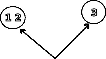
(a) An example of a non-free scattering state

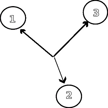
(b) A free scattering state

Figure 1: Examples of three-body scattering state profiles

We will now introduce the concept of channel wave operators, which are essential for capturing all asymptotic states. In the three-body system described in equation (1.1), a scattering state can either evolve as a free wave or follow a non-free scattering pattern, as depicted in Figures 1(a) and 1(b). Thus, this is a multi-channel problem, and we require multi-channel scattering theory. The key elements in this theory are the multi-channel wave operators, which play a crucial role in capturing all asymptotic states.

Definition 2 (Channel Wave Operators).

The channel wave operator for the $H_{a}$ channel is defined as:

$$\Omega_{a}^{*}\psi(0)=s\text{-}\lim_{t\to\infty}e^{itH_{a}}J_{a}e^{-itH}P_{sc}\psi(0),$$ (1.14)

where $\psi(0)\in\mathcal{H}=\mathcal{L}^{2}_{x}(\mathbb{R}^{9})$, and $P_{sc}$ represents the projection onto the space of all scattering states. The set ${H_{a}}$ refers to the collection of all sub-Hamiltonians of $H$, and ${J_{a}}$ is a set of smooth cut-off functions of $x$, $P$, and $t$ satisfying:

$$\sum_{a}J_{a}=1.$$ (1.15)

Our proof of the existence of all channel wave operators relies on the introduction of $J_{a}$, Assumption 1.1, and the dispersive estimates of the free flow of each particle. We will now detail the assumption associated with the dispersive estimate of the free flow for each particle. To be precise, we introduce $F(\lambda)$, $F_{c}(\lambda)$, and $F_{1}(\lambda)$ as smooth cutoff functions over the interval $[1,+\infty)$. We then define:

$$F(\lambda\leq a):=1-F(\lambda/a),\quad F_{c}(\lambda\leq a):=1-F_{c}(\lambda/a),\quad F_{1}(\lambda>a):=F_{1}(\lambda/a),$$ (1.16)

and

$$F_{c}(\lambda\leq a):=F_{c}(\lambda/a\leq 1):=1-F_{c}(\lambda/a),\quad F_{1}(\lambda\leq a):=F_{1}(\lambda/a\leq 1):=1-F_{1}(\lambda/a).$$ (1.17)

Furthermore, it’s posited that:

$$\begin{cases}F_{c}(k)=F_{1}(k)=F(k)=1&\text{ when }k\geq 1\\ F_{c}(k)=F_{1}(k)=F(k)=0&\text{ when }k\leq 1/2\end{cases}.$$ (1.18)

For operators $A_{j}$, where $j=1,\cdots,n$, we present the product $\Pi_{j=1}^{j=n}A_{j}$ as:

$$\Pi_{j=1}^{j=n}A_{j}=A_{1}\times A_{2}\times\cdots\times A_{n}$$ (1.19)

for operators $A_{j}$, $j=1,\cdots,n$. Throughout this paper, we maintain the assumption that for $j=1,2,3,$ $\omega_{j}(P_{j})$ adheres to the following:

Assumption 1.3.

Given $\eta_{jk}(k=1,\cdots,N_{j})$ as in (1.11), it is postulated that for every $j=1,2,3,$ an $\alpha>0$ exists such that for all $l\in\{1,2,3\}-\{j\}$,

$$E_{jl}:=\int_{1}^{\infty}dt\|F_{c,j,\alpha}(x_{j},t,P_{j})e^{it\omega_{j}(P_{j})}\langle x_{j}-x_{l}\rangle^{-5}\|_{\mathcal{L}^{2}_{x}(\mathbb{R}^{9})\to\mathcal{L}^{2}_{x}(\mathbb{R}^{9})}<\infty,$$ (1.20)

with

$$F_{c,j,\alpha}(x_{j},t,P_{j}):=F_{c}(|x_{j}|\leq t^{\alpha})\left(\Pi_{k=1}^{N_{j}}F_{1}(|P_{j}-\eta_{jk}|>\frac{1}{t^{\alpha/2}})\right)F_{1}(|P_{j}|\leq t^{\alpha/2}).$$ (1.21)

We define $E$ as:

$$E:=\max\limits_{j,l\in\{1,2,3\},j\neq l}E_{jl},$$ (1.22)

and setting

$$J_{a}=e^{-it\omega_{j}(P_{j})}F_{c,j,\alpha}(x_{j},t,P_{j})e^{it\omega_{j}(P_{j})}.$$ (1.23)

Remark 1.

Indeed, Assumption 1.3 can be derived using the non-stationary phase method, coupled with the fact that there exists only a finite number of vectors $\eta$ for which $\nabla_{\eta}[\omega_{j}(\eta)]=0$ $($where $j=1,2,3).$

We prove the existence of all channel wave operators under Assumptions 1.1, 1.2, and 1.3. Specifically, for every $a=(jk)(l)\in L$, and for all $\alpha$ that meet Assumption 1.3, the following holds:

$$\Omega_{a,\alpha}^{*}:=s\text{-}\lim\limits_{t\to\infty}F_{c,l,\alpha}(x_{l},t,P_{l})e^{itH_{a}}e^{-itH},\quad\text{ on }\mathcal{L}^{2}_{x}(\mathbb{R}^{9})$$ (1.24)

exists and the new free channel wave operator

$$\Omega_{free,\alpha}^{*}:=s\text{-}\lim\limits_{t\to\infty}\left(\Pi_{l=1}^{l=3}F_{c,l,\alpha}(x_{l},t,P_{l})\right)e^{itH_{0}}e^{-itH},\quad\text{ on }\mathcal{L}^{2}_{x}(\mathbb{R}^{9})$$ (1.25)

exists as well, where $F_{c,l,\alpha}(x_{l},t,P_{l})$ is defined in (1.21). We state this result formally in the following theorem:

Theorem 1.1.

If Assumptions 1.1, 1.2 and 1.3 are satisfied, then $\Omega_{a,\alpha}^{*}$ exists for all $a=(jk)(l)\in L$, and $\Omega_{free,\alpha}^{*}$ exists as well.

The proof of Theorem 1.1 is deferred to Section 3. According to Theorem 1.1, for each $a=(jk)(l)\in L_{sc}$, $\psi_{a}$ is given by

$$\psi_{a}=\Omega_{a,\alpha}^{*}\psi,$$ (1.26)

and when $a=(1)(2)(3)$,

$$\psi_{a}=\Omega_{free,\alpha}^{*}\psi.$$ (1.27)

A key element in proving Theorem 1.1 is the application of the propagation estimates from [SW1]. Here, we point out that if both $\alpha$ and $\alpha^{\prime}$ satisfy Assumption 1.3, then for all $a=(jk)(l)\in L$, we have

$$\Omega_{a,\alpha}^{*} =\Omega_{a,\alpha^{\prime}}^{*},$$

$$\Omega_{free,\alpha}^{*} =\Omega_{free,\alpha^{\prime}}^{*}.$$

In other word, both $\Omega_{a,\alpha}^{*}$ and $\Omega_{free,\alpha}^{*}$ are independent on the specific choice of $\alpha$. Instead of using $\Omega_{a,\alpha}^{*}$ and $\Omega_{free,\alpha}^{*}$, we employ $\Omega_{a}^{*}$ and $\Omega_{free}^{*}$, respectively. A detailed discussion can be found in Lemma 3.1. Based on the concept of channel wave operators, we introduce the channel projections as follows. For each $a=(jk)(l)\in L$,

$$P_{a}=s\text{-}\lim\limits_{t\to\infty}e^{itH}e^{-itH_{a}}F_{c,l,\alpha}(x_{l},t,P_{l})e^{itH_{a}}e^{-itH},\quad\text{ on }\mathcal{L}^{2}_{x}(\mathbb{R}^{9}),$$ (1.28)

and

$$P_{free}=s\text{-}\lim\limits_{t\to\infty}e^{itH}e^{-itH_{0}}\left(\Pi_{l=1}^{l=3}F_{c,l,\alpha}(x_{l},t,P_{l})\right)e^{itH_{0}}e^{-itH},\quad\text{ on }\mathcal{L}^{2}_{x}(\mathbb{R}^{9}).$$ (1.29)

Here, we omit the subscript $\alpha$ in both (1.28) and (1.29) since the channel projections are independent of $\alpha$ as well. See Lemma 3.3. The existence of $P_{a}$ and $P_{free}$ follow by using Cook’s method and propagation estimates introduced in [SW20221]. Please refer to the proof of Proposition 3.2 in Section 3.2 for a detailed discussion. We would also like to remind the reader that, based on the definition of $F_{c,j,\alpha}(x_{j},t,P_{j})$ in (1.21), the following identity holds for all $a=(jk)(l)\in L$:

$$e^{-itH_{a}}(1-F_{c,l,\alpha}(x_{l},t,P_{l}))e^{itH_{a}}=e^{-it\omega_{l}(P_{l})}(1-F_{c,l,\alpha}(x_{l},t,P_{l}))e^{it\omega_{l}(P_{l})}.$$ (1.30)

By employing (1.30), we can conclude that the existence of all channel projections, mentioned in (1.28) and (1.29), implies the existence of $P_{\mu}$:

$$P_{\mu}:=s\text{-}\lim\limits_{t\to\infty}e^{itH}\left(\Pi_{l=1}^{l=3}e^{-it\omega_{l}(P_{l})}(1-F_{c,l,\alpha}(x_{l},t,P_{l}))e^{it\omega_{l}(P_{l})}\right)e^{-itH}\quad\text{ on }\mathcal{L}^{2}_{x}(\mathbb{R}^{9}),$$ (1.31)

where $\alpha$ satisfies Assumption 1.3, see Propositions 3.2 and 3.3.

According to the statement in (1.13) and the formulations for $\psi_{a}$ given by (1.26) and (1.27), we can infer that if $P_{\mu}P_{sc}=0$, then AC holds true.

Theorem 1.2.

If $P_{\mu}P_{sc}=0$ and if Assumptions 1.1, 1.2, and 1.3 are satisfied, then AC holds for system (1.1).

Therefore, the challenge of proving AC is reduced to demonstrating that $P_{\mu}P_{sc}=0$. Before delving into the validity of $P_{\mu}P_{sc}=0$, let’s take a closer look at $P_{sc}.$ Once we establish Ruelle’s Theorem for system (1.1), we can provide a precise description of the space of all scattering states. This space is a subspace of $\mathcal{L}^{2}_{x}(\mathbb{R}^{9})$ and corresponds to the continuous spectrum of $H$ on each fiber. Its complement in $\mathcal{L}^{2}_{x}(\mathbb{R}^{9})$ is referred to as the space of all bound states or eigenfunctions. More specifically, the projection onto the space of all scattering states is given by the fiber integral $P_{sc}:\mathcal{L}^{2}_{x}(\mathbb{R}^{9})\to\mathcal{L}^{2}_{x}(\mathbb{R}^{9})$:

$$P_{sc}f=P_{c}(P_{1}+P_{2}+P_{3})f,$$ (1.32)

where $P_{c}(Q)$ denotes the projection onto the space of the continuous spectrum of $H$ with a total wave number operator $\sum\limits_{j=1}^{3}P_{j}=Q$ (Here, we use the fact that $[P_{1}+P_{2}+P_{3},H]=0$, which implies that the total wave number operator $\sum\limits_{j=1}^{3}P_{j}$ is invariant under the evolution of system (1.1)). For detailed information, please see Section 2.2. We refer to $\psi_{0}(x)\in\mathcal{L}^{2}_{x}(\mathbb{R}^{9})$ as a bound state of $H$ if it is orthogonal to all scattering states. Here, the space of all bound states, the complement of the space of all scattering states in $\mathcal{L}^{2}_{x}(\mathbb{R}^{9})$, is equal to the discrete spectrum of $H$ on each fiber. In quantum mechanics, an eigenfunction is commonly known as a bound state. For more details, please see Proposition 2.2 in Section 2.3.

Now, let’s discuss the validity of $P_{\mu}P_{sc}=0$. Interestingly, under further assumptions on the two-body sub-Hamiltonians, $P_{\mu}$ acts as the projection onto the space of all bound states. This claim is formally presented in Proposition 1.1, with its proof deferred to Sections 4 through 6. Before presenting Proposition 1.1, let’s first discuss the assumptions outlined within it. To begin with, the discussion about the assumptions requires the Feynman-Hellmann Theorem:

Theorem 1.3 (Feynman-Hellmann Theorem).

For $I=(a_{1},b_{1})\times\cdots(a_{m},b_{m})\subseteq\mathbb{R}^{m}$, let $\{H(p)\}_{p\in I}$ be a class of self-adjoint operators on $\mathcal{L}^{2}_{x}(\mathbb{R}^{n})$. Assume that $\lambda(p)$ is an eigenvalue of $H(p)$. If $H(p)$ is differentiable with respect to $p$, then $\lambda(p)$ is differentiable with respect to $p$ at $p=p_{0}$:

$$\frac{\partial\lambda(p)}{\partial p_{k}}|_{p=p_{0}}=(\psi_{\lambda},\frac{\partial H(p)}{\partial p_{k}}\psi_{\lambda})_{\mathcal{L}^{2}_{x}(\mathbb{R}^{n})}|_{p=p_{0}},\quad k=1,\cdots,m$$ (1.33)

where $\psi_{\lambda}$ stands for a normalized eigenfunction $(\|\psi_{\lambda}\|_{\mathcal{L}^{2}_{x}(\mathbb{R}^{n})}=1)$ with an eigenvalue $\lambda(p).$

It’s clear that the Feynman-Hellmann Theorem cannot be universally applied. Consider, for example, a family of parameterized operators denoted as $\{H(p)\}_{p\in I}$, where $H(p)=-\Delta_{x}+pW(x)$ and $p\in I=(-2,2)$. In this case, given $W(x)\leq 0$ to ensure that $-\Delta_{x}+W(x)$ has an eigenvalue $\lambda$ in $\mathcal{L}^{2}_{x}(\mathbb{R}^{n})$, it follows that $H(1)$ has an eigenvalue $\lambda(1):=\lambda$. However, $H(0)=-\Delta_{x}$ does not have an eigenvalue in $\mathcal{L}^{2}_{x}(\mathbb{R}^{n})$. This implies that the eigenvalue $\lambda(p)$ disappears at some $p\in(0,1)$. Thus, in such scenarios, the Feynman-Hellmann Theorem isn’t applicable across the entire index set $(-2,2)$. If the eigenvalue does not disappear at $p=p_{0}$, then we can apply the Feynman-Hellmann Theorem, and we say that the Feynman-Hellmann Theorem is applicable to this eigenvalue at $p=p_{0}$. In this note, we state that the Feynman-Hellmann Theorem is applicable to $\{H(p)\}_{p\in I}$ at $p=p_{0}$ if all eigenvalues of $H(p)$ are defined in a neighborhood of $p_{0}$ in $\mathbb{R}^{m}.$

Let’s now discuss the conditions under which an eigenvalue might disappear. To begin, let’s consider non-embedded eigenvalues. We refer to $\lambda$ as a non-embedded eigenvalue of a one-body self-adjoint Hamiltonian $H_{1}=\omega(P)+W(x)$ if $\lambda$ is an eigenvalue of $H_{1}$ and if

$$\lambda<\min\limits_{q\in\mathbb{R}^{3}}\omega(q).$$ (1.34)

Here, we refer to $\min\limits_{q\in\mathbb{R}^{3}}\omega(q)$ as the threshold energy of $\omega(P)$. Remarkably, we’ve found that the non-embedded eigenvalues of our two-body Hamiltonians, which can be simplified to one-body forms, vanish only as they near the threshold energy of $\omega(P)$. This is provided that both the position variable $x_{j}$ of the $j$th particle and the group velocity remains controlled when its energy is finite.

Assumption 1.4.

We assume that:

• $\omega_{j}(\eta)\to\infty$ as $|\eta|\to\infty$.

• For any $E\in\mathbb{R}$, we assume that for all $t\in\mathbb{R}$ and $d=1,2,3,4,$

  $$\|\langle x_{k}\rangle^{d}e^{itH^{a}(\eta)}F(H^{a}(\eta)<4E)\langle x_{k}\rangle^{-d}\|_{\mathcal{L}^{2}_{x_{k}}(\mathbb{R}^{3})\to\mathcal{L}^{2}_{x_{k}}(\mathbb{R}^{3})}\lesssim_{E}\langle t\rangle^{d}$$ (1.35)

  and

  $$\sup\limits_{s\in\mathbb{R}}\|\nabla_{\eta}[\omega_{j}(\eta-P_{k})]e^{isH^{a}(\eta)}F(H^{a}(\eta)<E)\|_{\mathcal{L}^{2}_{x_{k}}(\mathbb{R}^{3})\to\mathcal{L}^{2}_{x_{k}}(\mathbb{R}^{3})}\lesssim_{E}1$$ (1.36)

  hold true.

Remark 2.

We define $\psi\in\mathcal{L}^{2}$ to have a finite energy if $\psi=F(H\leq M)\psi$ for some $M\geq 1$. In Assumption 1.4, we assume that for $j=1,2,3,$ $\omega_{j}(\eta)\to\infty$ as $|\eta|\to\infty$. This is because we aim to establish that $P_{\mu}P_{sc}=0$ on $\mathcal{L}^{2}_{x}(\mathbb{R}^{9})$ by demonstrating $P_{\mu}P_{sc}\psi=0$ for every $\psi\in\mathcal{L}^{2}_{x}(\mathbb{R}^{9})$ with a finite energy.

Lemma 1.1.

If Assumptions 1.1 and 1.4 are valid, then all non-embedded eigenvalues of $H^{a}(\eta)=\omega_{j}(\eta-P_{k})+\omega_{k}(P_{k})+V_{jk}(-x_{k})$, for $a=(jk)(l)\in L$ and $\eta\in\mathbb{R}^{3}$, disappear at threshold points of $H^{a}(\eta)$.

We defer the proof of Lemma 1.1 to subsection 2.4.2. We refer to $E\in\mathbb{R}$ as a threshold point of the one-body Hamiltonian $H_{1}$ if $E=\omega(\eta_{0})$ with $\nabla_{\eta}[\omega(\eta)]|_{\eta=\eta_{0}}=0.$ Then the threshold energy of $\omega(P)$ is a threshold point of $H_{1}$. We know that a two-body Hamiltonian can be simplified to a one-body Hamiltonian through a coordinate transformation. Assuming the eigenvalues of all two-body sub-Hamiltonians in our three-body Hamiltonian $H$ do not reach threshold points, the embedded eigenvalues of these two-body sub-Hamiltonians will not disappear. This assumption, that all threshold points of a two-body Hamiltonian are neither an eigenvalue nor a resonance, is also termed the regularity assumption for the two-body Hamiltonian. Here, a resonance of a one-body Hamiltonian $H_{1}$ is a distributional solution of $H_{1}\psi=0$ such that $\psi\notin\mathcal{L}^{2}_{x}$ but $\langle x\rangle^{-\sigma}\psi\in\mathcal{L}^{2}_{x}$ for some $\sigma>0$. Refer to [JK1979] for one-body Schrödinger operators.

Assumption 1.5.

All threshold points are neither an eigenvalue nor a resonance of $H^{a}(\eta):=\omega_{j}(\eta-P_{k})+\omega_{k}(P_{k})+V_{jk}(-x_{k})$ for all $\eta\in\mathbb{R}^{3}$ and $a=(jk)(l)\in L$.

Under Assumption 1.5, due to Lemma 1.1, we conclude that all non-embedded eigenvalues of $H^{a}(\eta)$, for $\eta\in\mathbb{R}^{3},a=(jk)(l)\in L$, will not disappear and Feynman-Hellmann Theorem is then applicable. Consequently, we can express the projection onto the space of all eigenfunctions with non-embedded eigenvalues of $H^{a}(\eta)$ as

$$P_{b}(H^{a}(\eta))=\sum\limits_{d=1}^{\tilde{N}^{a}}\tilde{P}_{b,d}(H^{a}(\eta))$$ (1.37)

where $\tilde{N}^{a}=\tilde{N}^{a}(a)\in\mathbb{N}$ is independent on $\eta\in\mathbb{R}^{3}$. Here, for $d=1,\cdots,\tilde{N}^{a}$, $\tilde{P}_{b,d}(H^{a}(\eta))$ denotes rank-one projection with an eigenvalue $\lambda_{a,d}(\eta)$. We say that for $1\leq d_{1}<d_{2}\leq\tilde{N}^{a}$ $\lambda_{a,d1}\neq\lambda_{a,d2}$ if $\lambda_{a,d_{1}}(\eta)\neq\lambda_{a,d_{2}}(\eta)$ for some $\eta\in\mathbb{R}^{3}$. Otherwise, we say that $\lambda_{a,d_{1}}$ and $\lambda_{a,d_{2}}$ are the same. By putting the rank-one projections $\tilde{P}_{b,d}(H^{a}(\eta))$ with the same $\lambda_{a,d}$(same for all $\eta\in\mathbb{R}^{3}$) into one projection, we get

$$P_{b}(H^{a}(\eta))=\sum\limits_{d=1}^{N^{a}}P_{b,d}(H^{a}(\eta))$$ (1.38)

where $N^{a}=N^{a}(a)\in\mathbb{N}$ denotes the number of distinct $\lambda_{a,d}$.

Remark 3.

Here, we have both $\tilde{N}^{a}$ and $N^{a}$ are finite for all $a=(jk)(l)\in L$. This arises due to (1.54) as presented in Assumption 1.10, which will be detailed later. Put simply, when all eigenfunctions are both smooth and spatially localized as suggested by (1.10), the dimension of the space containing all eigenfunctions of $H^{a}(\eta)$ remains finite for all $\eta\in\mathbb{R}^{3},a=(jk)(l)\in L$. This is because $\langle x\rangle^{-4}\langle P\rangle^{-4}$ is a compact operator on $\mathcal{L}^{2}_{x}(\mathbb{R}^{n})$ for all $n=1,2,\cdots.$ It’s also noteworthy that for a one-body Schrödinger operator, $H_{1}=-\Delta_{x}+W(x)$, given some constant $b>0$, if the potential $W(x)\geq-\frac{b}{4}|x|^{-2}$ for $|x|\geq R$ with some sufficiently large $R\geq 1$, then $H_{1}$ has at most finitely many eigenvalues. See Theorem XIII.6 on page 87 in [RS1978].

For simplicity, we assume that for all $\eta\in\mathbb{R}^{3}$, $a=(jk)(l)\in L$, $d_{1},d_{2}\in\{1,2,3\}$ and $l_{1},l_{2}\in\{0,1\}$, we have

$$\mathscr{C}_{a,b}:=\sum\limits_{l_{1}=0}^{1}\sum\limits_{l_{2}=0}^{1}\|\partial_{\eta_{d_{1}}}^{l_{1}}\partial_{\eta_{d_{2}}}^{l_{2}}[P_{b,d}(H^{a}(\eta))]\|_{\mathcal{L}^{2}_{x_{k}}(\mathbb{R}^{3})\to\mathcal{L}^{2}_{x_{k}}(\mathbb{R}^{3})}\lesssim 1.$$ (1.39)

Assumption 1.6.

For all $\eta\in\mathbb{R}^{3}$, $a=(jk)(l)\in L$, $d_{1},d_{2}\in\{1,2,3\}$ and $l_{1},l_{2}\in\{0,1\}$, (1.39) is valid.

Now let us discuss the embedded eigenvalues of $H^{a}$ for $a=(jk)(l)\in L$. In the context of a one-body Hamiltonian, the Fermi’s golden rule (as discussed in [SW1998], for instance) indicates that these embedded eigenvalues are unstable. This means that adding a small perturbation, the embedded eigenvalues go away. Let

$$I_{a,em}:=\{\eta\in\mathbb{R}^{3}:H^{a}(\eta)\text{ has an embedded eigenvalue}\}.$$ (1.40)

For simplicity, we assume that $I_{a,em}$ is contained in the union of fintely many hypersurfaces of $\mathbb{R}^{3}$:

Assumption 1.7.

For all $a=(jk)(l)\in L$, $I_{a,em}$ is contained in the union of fintely many hypersurfaces of $\mathbb{R}^{3}$.

Given Assumption 1.7, we infer that for all $a=(jk)(l)\in L$, $P_{b}(H^{a})$ can be viewed as the projection onto the space of all bound states of $H^{a}$ in $\mathcal{L}^{2}_{x}(\mathbb{R}^{9})$.

We now turn our attention to the assumptions made on all two-body sub-Hamiltonians. We begin with the introduction of cut-off functions of operators. Let us consider a finite set $A=\{a_{1},\cdots,a_{n}\}\subseteq\mathbb{R}$. For any given $y\in\mathbb{R}$, we define

$$[y-A]_{d}:=(y-a_{1},\cdots,y-a_{n}).$$ (1.41)

Given any $c\in(0,1)$, we introduce the following notation

$$\bar{F}([y-A]_{d},c):=\left(\Pi_{j=1}^{j=n}F(|y-a_{j}|>c)\right)\times F(|y|\leq\frac{1}{c}).$$ (1.42)

When $A=\emptyset$, we adopt

$$\bar{F}([y-A]_{d},c):=F(|y|\leq\frac{1}{c}).$$ (1.43)

Here, $\bar{F}$ means ”away”. In other word, in the support of $\bar{F}([y-A]_{d},c)$, the value of $y$ is bounded and it is distinctly separated from the set $A$ by a distance greater than $c/2$. Let’s also consider a family of finite sets in $\mathbb{R}$, represented as $\{S(p)\}_{p\in\mathbb{R}^{3}}$. When $n\geq 2$, we define $H_{n}$ as a quasi-$n$-particle Hamiltonian: $H_{n}=\sum\limits_{j=1}^{n}\omega_{j}(P_{j})+V(x)$ where for $j=1,\cdots,n$, $x_{j}\in\mathbb{R}^{3}$, $P_{j}:=-i\nabla_{x_{j}}$ and

$$V(x)=\sum\limits_{1\leq j<l\leq n}V_{jl}(x_{j}-x_{l}).$$ (1.44)

For a given $c>0$ and any quasi-$n$-particle Hamiltonian $H_{n}$(where $n=2,3$), we define

$$\bar{F}_{S,n}(H_{n},c):=\bar{F}([H_{n},S(\sum\limits_{j=1}^{n}P_{j})]_{d},c)F(|\sum\limits_{j=1}^{n}P_{j}|\leq\frac{1}{c}).$$ (1.45)

Moreover, we define $F_{S,n}:=1-\bar{F}_{S,n}$ for $n=2,3$. To express the asymptotic relative velocity between particle $j$ and particle $k$, we introduce the notion $v_{a}$, given $a=(jk)(l)\in L$. This is defined by

$$v_{a}:=\Omega^{a}(v_{j}(P_{j})-v_{k}(P_{k}))\Omega^{a,*},$$ (1.46)

where $\Omega^{a}:=s\text{-}\lim\limits_{t\to\infty}e^{itH_{a}}e^{-itH_{0}}$ and $\Omega^{a,*}$ stands for the conjugate of $\Omega^{a}$. For $a=(jk)(l)\in L$ and $\eta\in\mathbb{R}^{3}$, let $P_{c}(H^{a}(\eta))$ denote the projection on the space of the continuous spectral subspcae of $H^{a}(\eta)$. We define $P_{c}(H^{a})$ as $P_{c}(H^{a}(P_{j}+P_{k}))$. Roughly speaking, our Assumption 1.8 is that when we fix $\sum\limits_{j=1}^{3}P_{j}$, except for a finite number of points, the magnitude of $|v_{a}|$ is approximately $|P_{j}-P_{k}|$ when $P_{j}$ is close to $P_{k}$. Furthermore, we assume that both $e^{-itH_{a}}P_{c}(H^{a})$ and $e^{-itH_{0}}$ adhere to local decay estimates in a manner similar to how $e^{-it(-\Delta)}$ does.

Assumption 1.8.

For all $a=(jk)(l)\in L$, we assume that there exists a collection of finite sets in $\mathbb{R}$ denoted by $\{I_{a}(p)\}_{p\in\mathbb{R}^{3}}$, with $\sup\limits_{p\in\mathbb{R}^{3}}|I_{a}(p)|<\infty,$ such that for all $\beta>0$ and some $C=C(c)>0$

$$\|\langle x_{j}-x_{k}\rangle^{-2}F(|v_{a}|\leq\langle t\rangle^{-\beta})\bar{F}_{I_{a},3}(H_{a},c)\|_{\mathcal{L}^{2}_{x}(\mathbb{R}^{9})\to\mathcal{L}^{2}_{x}(\mathbb{R}^{9})}\leq\frac{C}{\langle t\rangle^{3\beta/2}},$$ (1.47)

$$\|\langle x_{k}-x_{j}\rangle^{-2}e^{-itH_{a}}\bar{F}_{I_{a},3}(H_{a},c)P_{c}(H^{a})\langle x_{k}-x_{j}\rangle^{-2}\|_{\mathcal{L}^{2}_{x}(\mathbb{R}^{9})\to\mathcal{L}^{2}_{x}(\mathbb{R}^{9})}\leq\frac{C}{\langle t\rangle^{3/2}}$$ (1.48)

and

$$\|\langle x_{j}-x_{k}\rangle^{-2}e^{-itH_{0}}\bar{F}_{I_{a},3}(H_{0},c)\|_{\mathcal{L}^{2}_{x}(\mathbb{R}^{9})\to\mathcal{L}^{2}_{x,t}(\mathbb{R}^{9+1})}\leq C.$$ (1.49)

Remark 4.

Assumption 1.8 indicates that when we fix the $\sum\limits_{j=1}^{3}P_{j}$, aside from a finite number of energy values, all two-body sub-Hamiltonians and the free flow exhibit normal decay estimates similar to those seen with Schrödinger operators. For Schrödinger operators, an estimate like (1.49) follows from the local resolvent estimate: for some $C=C(c)>0$

$$\|\langle x_{j}-x_{k}\rangle^{-2}\frac{1}{H_{0}-y\pm i0}\bar{F}_{I_{a},3}(H_{0},c)\|_{\mathcal{L}^{2}_{x}(\mathbb{R}^{9})\to\mathcal{L}^{2}_{x,y}(\mathbb{R}^{9+1})}\leq C.$$ (1.50)

See [CS1988].

Using a pointwise in time local decay estimate, as given in (1.48), we can obtain further results, including resolvent estimates and minimum velocity bounds for Schrödinger operators. Refer to [HSS1999] for details on the minimum velocity bounds for Schrödinger operators. For a one-body Schrödinger operator, it is also well-known that if $0$ is neither an eigenvalue nor a resonance and if the potential $W(x)$ is well-localized (e.g. $|W(x)|\leq\frac{C}{\langle x\rangle^{2+\epsilon}}$ for some $\epsilon>0$ and constant $C>0$), the dimension of the space of all eigenfunctions is finite and all eigenfunctions are localized in space variable $x$. These outcomes can be analogously derived for the general one-body Hamiltonian. For the sake of clarity in this note, we choose to assume these results, which can be validated using known techniques, in Assumption 1.10. We defer their proofs to a subsequent paper. We assume that the set of all threshold points of $H^{a}(\eta)$(where $\eta\in\mathbb{R}^{3}$ and $a=(jk)(l)\in L$) are finite uniformly in $\eta\in\mathbb{R}^{3}$ as well.

Assumption 1.9.

For $a=(jk)(l)\in L$, let

$$I_{aE}(\eta):=\{E:E=\omega_{j}(\eta-q_{k})+\omega_{k}(q_{k}),\nabla_{q_{k}}[\omega_{j}(\eta-q_{k})+\omega_{k}(q_{k})]=0\},\quad\text{for }\eta\in\mathbb{R}^{3}.$$ (1.51)

We postulate the existence of a positive integer $N$ such that $|I_{aE}|\leq N<\infty$.

Assumption 1.10.

For $a=(jk)(l)\in L$, let $I_{a},I_{aE}$ be as in Assumptions 1.8 and 1.9, respectively. We further assume the existence of constants $C_{1}=C_{1}(c,\epsilon)>0$ and $C_{2}=C_{2}(c)>0$ such that

$$\|\langle x_{k}-x_{j}\rangle^{-2}e^{-itH_{a}}\bar{F}_{S,3}(H_{a},c)P_{c}(H^{a})F(|v_{a}|>\frac{1}{\langle t\rangle^{1/2-\epsilon}})\langle x_{k}-x_{j}\rangle^{-2}\|_{\mathcal{L}^{2}_{x}(\mathbb{R}^{9})\to\mathcal{L}^{2}_{x}(\mathbb{R}^{9})}\leq\frac{C_{1}}{\langle t\rangle^{3/2}},$$ (1.52)

$$\|\langle x_{j}-x_{k}\rangle^{-2}e^{-itH_{a}}\bar{F}_{S,3}(H_{a},c)\|_{\mathcal{L}^{2}_{x}(\mathbb{R}^{9})\to\mathcal{L}^{2}_{x,t}(\mathbb{R}^{9+1})}\leq C_{2}$$ (1.53)

and

$$\|\langle P_{k}\rangle^{4}\langle x_{k}\rangle^{4}P_{b,d}(H^{a}(\eta))\|_{\mathcal{L}^{2}_{x_{k}}(\mathbb{R}^{3})\to\mathcal{L}^{2}_{x_{k}}(\mathbb{R}^{3})}\lesssim 1,$$ (1.54)

where $d=1,\cdots,N^{a}$. Additionally, we assume that for all values $c>0$, $\sigma\in(0,4]$, $\epsilon\in(0,1/2)$ and $M\geq 1$,

$$\|\langle x_{j}-x_{k}\rangle^{-\sigma}\bar{F}_{I_{aE},2}(H^{a},c)e^{-itH_{a}}P_{c}(H^{a})\langle x_{j}-x_{k}\rangle^{-\sigma}\|_{\mathcal{L}^{2}_{x}(\mathbb{R}^{9})\to\mathcal{L}^{2}_{x}(\mathbb{R}^{9})}\leq\frac{C}{\langle t\rangle^{\sigma}},$$ (1.55)

and

$$\|F(|x_{l}-x_{j}|\geq M)\langle x_{j}-x_{k}\rangle^{-\sigma}F(|v_{a}|>\frac{1}{\langle t\rangle^{1/2-\epsilon}})F_{S,2}(H^{a},c)e^{-itH_{a}}$$

$$\times\langle x_{j}-x_{l}\rangle^{-\sigma}\chi(|x_{j}-x_{k}|\leq\langle t\rangle^{1/2})\|_{\mathcal{L}^{2}_{x}(\mathbb{R}^{9})\to\mathcal{L}^{2}_{x}(\mathbb{R}^{9})}$$

$$\leq\frac{C}{\langle t+M\rangle^{\sigma/2}}$$ (1.56)

hold true for some constants $C_{3}=C_{3}(c)>0$ and $C_{4}=C_{4}(\epsilon)>0$.

Let’s return to the statement $P_{\mu}P_{sc}=0$. Our approach to prove this is as follows: when $\sum\limits_{j=1}^{3}P_{j}=v_{T}$ is fixed, we aim to identify a finite set of points such that if the energy of the $\mathcal{L}^{2}$ data $\psi$ is away from these finitely many values, then $P_{\mu}P_{sc}\psi=0$. We refer to these finitely many points as threshold points of $H$. We will now discuss the assumptions required to ensure that, for a given total momentum $v_{T}\in\mathbb{R}^{3}$, the set of all threshold points for $H$(defined in subsection 2.4) is finite. Given a finite set $A\subseteq\mathbb{R}$, we let $|A|$ denote the cardinality of elements in $A$.

Assumption 1.11.

We assume that for all $v_{T}\in\mathbb{R}^{3}$, the set

$$\tau_{free}(v_{T}):=\{(q_{1},q_{2},q_{3})\in\mathbb{R}^{9}:v_{1}(q_{1})=v_{2}(q_{2})=v_{3}(q_{3}),\sum\limits_{j=1}^{3}q_{j}=v_{T}\}$$ (1.57)

is finite with

$$\sup\limits_{v_{T}\in\mathbb{R}^{3}}|\tau_{free}(v_{T})|<\infty.$$ (1.58)

According to Assumptions 1.2, 1.8, 1.9 and 1.11, we prove that when $\sum\limits_{j=1}^{3}P_{j}=v_{T}\in\mathbb{R}^{3}$ is fixed, the set of the threshold points for $H$(defined in subsection 2.4) is finite. Let $\tau(v_{T})$ denote the set of all threshold points for $H$ when $\sum\limits_{j=1}^{3}P_{j}=v_{T}\in\mathbb{R}^{3}$.

Lemma 1.2.

If Assumptions 1.2, 1.8, 1.9 and 1.11 hold, then there exists a positive integer $N$ such that $|\tau(v_{T})|\leq N$ for all $v_{T}\in\mathbb{R}^{3}$ and all $a=(jk)(l)\in L$.

We defer the proof of Lemma 1.2 to subsection 2.4.

We’re now ready to present the final assumption. Given the explanations that follow, we consider this assumption to be reasonable. Let $C_{1},C_{2}\in\mathbb{R}$ two distinct constants. If $H_{a}$ is very close to $C_{1}$ and $H_{0}$ is very close to $C_{2}$, then roughly speaking, $V_{jk}(x_{j}-x_{k})=H_{a}-H_{0}$ should be strictly away from $0$. This implies that it occurs in a region where $|x_{j}-x_{k}|$ is bounded. Similarly, if $H_{a}$ is very close to $C_{1}$ and $H$ is very close to $C_{2}$, then roughly speaking, $V_{jl}(x_{j}-x_{l})+V_{kl}(x_{k}-x_{l})=H-H_{a}$ should be strictly away from $0$. This indicates that this situation happens in the region where either $|x_{j}-x_{l}|$ or $|x_{k}-x_{l}|$ is bounded. Now, let’s delve into the details of this assumption. For each $a=(jk)(l)\in L$, we define $\mathcal{L}^{2}_{a}(\mathbb{R}^{9})$ as a Banach space:

$$\{f(x):f=f_{1}+f_{2},\text{ for some }f_{1},f_{2}\text{ with }\|\langle x_{j}-x_{l}\rangle^{3}f_{1}\|_{\mathcal{L}^{2}_{x}(\mathbb{R}^{9})},\|\langle x_{k}-x_{l}\rangle^{3}f_{2}\|_{\mathcal{L}^{2}_{x}(\mathbb{R}^{9})}\},$$ (1.59)

endowed with the norm:

$$\|f\|_{\mathcal{L}^{2}_{a}(\mathbb{R}^{9})}:=\inf\limits_{(f_{1},f_{2})\in Ind_{f}}\|\langle x_{j}-x_{l}\rangle^{3}f_{1}\|_{\mathcal{L}^{2}_{x}(\mathbb{R}^{9})}+\|\langle x_{k}-x_{l}\rangle^{3}f_{2}\|_{\mathcal{L}^{2}_{x}(\mathbb{R}^{9})},$$ (1.60)

where $Ind_{f}$ denotes the set of all $(f_{1},f_{2})$ such that $f=f_{1}+f_{2}$ with $\langle x_{j}-x_{l}\rangle^{3}f_{1},\langle x_{k}-x_{l}\rangle^{3}f_{2}\in\mathcal{L}^{2}_{x}(\mathbb{R}^{9}).$ Let $\tau^{a}(\eta)$ be the set of all threshold points of $H^{a}(\eta)$, as defined in Definition 14 in Section 2.4. Given Assumption 1.9, we also find that $\sup\limits_{v_{T}\in\mathbb{R}^{3}}|\tau^{a}(v_{T})|<\infty.$ Recall that in Lemma 1.2, we also have $\sup\limits_{v_{T}\in\mathbb{R}^{3}}|\tau(v_{T})|<\infty$. Given that these threshold points are finite within each fiber, we introduce the subsequent assumption.

Assumption 1.12.

We assume that for all $a=(jk)(l)\in L$ and $c>0$, we have:

• $$\|\langle x_{j}-x_{k}\rangle^{3}\bar{F}_{\tau}(H_{a},c)F_{\tau}(H_{0},\frac{c}{10})\|_{\mathcal{L}^{2}_{x}(\mathbb{R}^{9})\to\mathcal{L}^{2}_{x}(\mathbb{R}^{9})}\lesssim_{c}1,$$ (1.61)

  and

  $$\|\langle x_{j}-x_{k}\rangle^{3}F_{\tau^{a}}(H^{a},c)\bar{F}_{\tau^{a}}(H_{0}^{a},10c)\|_{\mathcal{L}^{2}_{x}(\mathbb{R}^{6})\to\mathcal{L}^{2}_{x}(\mathbb{R}^{6})}\lesssim_{c}1,$$ (1.62)

  where $H^{a}_{0}:=H_{0}-\omega_{l}(P_{l})$.

• $$\|\bar{F}_{\tau}(H_{a},c)F_{\tau}(H,\frac{c}{10})\|_{\mathcal{L}^{2}_{x}(\mathbb{R}^{9})\to\mathcal{L}^{2}_{a}(\mathbb{R}^{9})}\lesssim_{c}1,$$ (1.63)

  and

  $$\|F_{\tau}(H_{a},c)\bar{F}_{\tau}(H,10c)\|_{\mathcal{L}^{2}_{x}(\mathbb{R}^{9})\to\mathcal{L}^{2}_{a}(\mathbb{R}^{9})}\lesssim_{c}1.$$ (1.64)

Proposition 1.1.

If Assumptions 1.1 to 1.12 hold, then $P_{\mu}P_{sc}=0$ and $(1-P_{\mu})P_{sc}=P_{sc}$.

Furthermore, we use Proposition 1.1 as a basis for introducing a new method of defining the projection onto the space of all bound states:

Definition 3 (A new characterization of the projection on the space of all $3$-body bound states).

Let $\alpha$ be as in Assumption 1.3. The projection on the space of all $3$-body bound states is defined by

$$P_{\mu}:=s\text{-}\lim\limits_{t\to\infty}e^{itH}[\Pi_{j=1}^{j=3}e^{-it\omega_{j}(P_{j})}(1-F_{c,j,\alpha}(x,t,P))e^{it\omega_{j}(P_{j})}]e^{-itH}\quad\text{ on }\mathcal{L}^{2}_{x}(\mathbb{R}^{9}).$$ (1.65)

To continue our analysis, we require the concept of following projections. Given $a=(jk)(l),b=(j^{\prime}k^{\prime})(l^{\prime})\in L$, we define the following:

$$\mathscr{P}^{l^{\prime}}_{l}:=s\text{-}\lim\limits_{t\to\infty}e^{itH_{b}}e^{-itH_{a}}F_{c,l,\alpha}(x_{l},t,P_{l})e^{itH_{a}}e^{-itH_{b}},\quad\text{ on }\mathcal{L}^{2}_{x}(\mathbb{R}^{9}),$$ (1.66)

$$P_{sc}(H_{a}):=s\text{-}\lim\limits_{t\to\infty}e^{itH_{a}}e^{-itH_{0}}F_{c,j,\alpha}(x_{j},t,P_{j})e^{itH_{0}}e^{-itH_{a}},\quad\text{ on }\mathcal{L}^{2}_{x}(\mathbb{R}^{9})$$ (1.67)

and

$$P_{bs}(H_{a}):=1-P_{sc}(H_{a}).$$ (1.68)

Proposition 1.2.

If Assumptions 1.1, 1.2 and 1.3 hold, then $\mathscr{P}_{l}^{l^{\prime}},P_{sc}(H_{a}),P_{bs}(H_{a})$ and $\Omega_{\alpha}^{a,*}$ exist for all $a=(jk)(l),b=(j^{\prime}k^{\prime})(l^{\prime})\in L-\{(1)(2)(3)\}$.

The proof of Proposition 1.2 follows, similarly, by using Cook’s method and propagation estimates, as detailed in Section 3.

Based on Theorem 1.1, Proposition 1.1 and Proposition 1.2, we arrive at our main result in this note:

Theorem 1.4.

If Assumptions 1.1 to 1.12 hold, then we have AC for system (1.1): for all $\psi(0)=P_{sc}\psi(0)\in\mathcal{L}^{2}_{x}(\mathbb{R}^{9})$, we have

$$\lim\limits_{t\to\infty}\|\psi(t)-\sum\limits_{a\in L}e^{-itH_{a}}\psi_{a,+}(x)\|_{\mathcal{L}^{2}_{x}(\mathbb{R}^{9})}=0,$$ (1.69)

where for all $a\in L$, $\psi_{a,+}(x)$ are given by:

For $$a_{0}=(1)(2)(3) a_{l}=(jk)(l)\in L$$, ,

$$\psi_{a_{0},+}=\Omega^{a_{1},*}\Omega_{a_{1}}^{*}\psi_{0}+\Omega^{a_{2},*}(1-\mathscr{P}_{1}^{2})\Omega_{a_{2}}^{*}\psi_{0}+\Omega^{a_{3},*}(1-\mathscr{P}_{1}^{3})(1-\mathscr{P}_{2}^{3})\Omega_{a_{3}}^{*}\psi_{0},$$ (1.70a)

$$\psi_{a_{1},+}:=P_{bs}(H_{a_{1}})\Omega_{a_{1}}^{*}\psi_{0},$$ (1.70b)

$$\psi_{a_{2},+}:=P_{bs}(H_{a_{2}})(1-\mathscr{P}_{1}^{2})\Omega_{a_{2}}^{*}\psi_{0}$$ (1.70c)

and

$$\psi_{a_{3},+}:=P_{bs}(H_{a_{3}})(1-\mathscr{P}_{1}^{3})(1-\mathscr{P}_{2}^{3})\Omega_{a_{3}}^{*}\psi_{0}.$$ (1.70d)

Proof of Theorem 1.4.

We define

$$a_{1}=(23)(1),\quad a_{2}=(13)(2)\text{ and }a_{3}=(12)(3).$$ (1.71)

For $a=(jk)(l)\in L$, we set

$$J_{\alpha,a}(t):=e^{-itH_{a}}F_{c,l,\alpha}(x_{l},t,P_{l})e^{itH_{a}}.$$ (1.72)

We choose $\psi(0)=\psi_{0}=P_{sc}\psi_{0}\in\mathcal{L}^{2}_{x}(\mathbb{R}^{9})$. We can write the solution $\psi(t)=e^{-itH}\psi_{0}$ as

$$e^{-itH}\psi_{0}= J_{\alpha,a_{1}}(t)e^{-itH}\psi_{0}+(1-J_{\alpha,a_{1}}(t))J_{\alpha,a_{2}}(t)e^{-itH}\psi_{0}$$

$$+(1-J_{\alpha,a_{1}}(t))(1-J_{\alpha,a_{2}}(t))J_{\alpha,a_{3}}(t)e^{-itH}\psi_{0}$$

$$+(1-J_{\alpha,a_{1}}(t))(1-J_{\alpha,a_{2}}(t))(1-J_{\alpha,a_{3}}(t))e^{-itH}\psi_{0}.$$ (1.73)

Using Theorem 1.1 and Proposition 1.1, we have that as $t\to\infty$:

$$\|(1-J_{\alpha,a_{1}}(t))(1-J_{\alpha,a_{2}}(t))(1-J_{\alpha,a_{3}}(t))e^{-itH}\psi_{0}\|_{\mathcal{L}^{2}_{x}(\mathbb{R}^{9})}\to 0$$ (1.74)

and

$$\|e^{-itH}\psi_{0}-e^{-itH_{a_{1}}}\Omega_{a_{1}}^{*}\psi_{0}-\psi_{\alpha,2}(t)\|_{\mathcal{L}^{2}_{x}(\mathbb{R}^{9})}\to 0,$$ (1.75)

where

$$\psi_{\alpha,2}(t):=(1-J_{\alpha,a_{1}}(t))e^{-itH_{a_{2}}}\Omega_{a_{2}}^{*}\psi_{0}+(1-J_{\alpha,a_{1}}(t))(1-J_{\alpha,a_{2}}(t))e^{-itH_{a_{3}}}\Omega_{a_{3}}^{*}\psi_{0}.$$ (1.76)

Using Proposition 1.2, we have that as $t\to\infty$:

$$\|(1-J_{\alpha,a_{1}}(t))e^{-itH_{a_{2}}}\Omega_{a_{2}}^{*}\psi_{0}-e^{-itH_{a_{2}}}(1-\mathscr{P}_{1}^{2})\Omega_{a_{2}}^{*}\psi_{0}\|_{\mathcal{L}^{2}_{x}(\mathbb{R}^{9})}\to 0,$$ (1.77)

and

$$\|(1-J_{\alpha,a_{1}}(t))(1-J_{\alpha,a_{2}}(t))e^{-itH_{a_{3}}}\Omega_{a_{3}}^{*}\psi_{0}-e^{-itH_{a_{3}}}(1-\mathscr{P}_{1}^{3})(1-\mathscr{P}_{2}^{3})\Omega_{a_{3}}^{*}\psi_{0}\|_{\mathcal{L}^{2}_{x}(\mathbb{R}^{9})}\to 0.$$ (1.78)

Proposition 1.2 implies that (1.69) holds by choosing

$$\psi_{a_{0},+}=\Omega^{a_{1},*}\Omega_{a_{1}}^{*}\psi_{0}+\Omega^{a_{2},*}(1-\mathscr{P}_{1}^{2})\Omega_{a_{2}}^{*}\psi_{0}+\Omega^{a_{3},*}(1-\mathscr{P}_{1}^{3})(1-\mathscr{P}_{2}^{3})\Omega_{a_{3}}^{*}\psi_{0},$$ (1.79)

$$\psi_{a_{1},+}:=P_{bs}(H_{a_{1}})\Omega_{a_{1}}^{*}\psi_{0},$$ (1.80)

$$\psi_{a_{2},+}:=P_{bs}(H_{a_{2}})(1-\mathscr{P}_{1}^{2})\Omega_{a_{2}}^{*}\psi_{0}$$ (1.81)

and

$$\psi_{a_{3},+}:=P_{bs}(H_{a_{3}})(1-\mathscr{P}_{1}^{3})(1-\mathscr{P}_{2}^{3})\Omega_{a_{3}}^{*}\psi_{0}.$$ (1.82)

We finish the proof. ∎

2 Basic dynamics

Let $\mathcal{L}^{2}(X_{v_{T}})$ be the space of all $\mathcal{L}^{2}$ functions with $\sum\limits_{j=1}^{3}P_{j}=v_{T}$, where $v_{T}\in\mathbb{R}^{3}$ is fixed. $\mathcal{L}^{2}(X_{v_{T}})$ is a fiber Hilbert space, which we will delve into later in this section. This section focuses on configuration space and three key properties of Schrödinger operators $H$ on the fiber Hilbert space $\mathcal{L}^{2}(X_{v_{T}})$: self-adjointness, Ruelle’s theorem, and the set of all threshold points for $H$. By using Ruelle’s theorem in $\mathcal{L}^{2}(X_{v_{T}})$, we get a Ruelle’s theorem in $\mathcal{L}^{2}_{x}(\mathbb{R}^{9})$. We can not get the Ruelle’s theorem in $\mathcal{L}^{2}_{x}(\mathbb{R}^{9})$ directly because, in the region where $|x_{1}-x_{2}|$, $|x_{1}-x_{3}|$, and $|x_{2}-x_{3}|$ are bounded, there exist points $x\in\mathbb{R}^{9}$ for which $|x|$ goes to infinity. Throughout this section, we assume the validity of Assumptions 1.1- 1.11. The structure of this section follows [HS1].

2.1 Configuration space

Given that $[P_{1}+P_{2}+P3,H]=0$, the total quasi-momentum of the three particles is conserved under the flow $e^{-itH}$ of the system (1.1). By decomposing $\mathcal{L}^{2}_{x}(\mathbb{R}^{9})$ based on the total quasi-momentum, we obtain the fiber space, $\mathcal{L}^{2}(X_{v_{T}})$, which is the $\mathcal{L}^{2}$ space associated with a total quasi-momentum $v_{T}$.

2.1.1 The fiber Hilbert space

The configuration space $X$ of a quasi-three-particle system is a Euclidean space with scalar product denoted by $x\cdot y$. Specifically, we have

$$X\equiv\mathbb{R}^{9}\quad\text{ and }\quad x\cdot y\equiv\sum\limits_{j=1}^{3}(x_{j}\cdot y_{j})_{\mathbb{R}^{3}}.$$ (2.1)

The quasi-momentum conjugate to $X,$ is denoted by $p$. In quantum mechanics, this quasi-momentum has the conventional form in Cartesian coordinates (not particle coordinates) of $X$, which is given by $p=-i\nabla_{x}$. For a given $v_{T}\in\mathbb{R}^{3}$, we introduce $P_{v_{T}}$ as a framework representing the total quasi-momentum $v_{T}$. This can be symbolically expressed as:

$$P_{v_{T}}\equiv\{p=(p_{1},p_{2},p_{3}):p_{j}\in\mathbb{R}^{3}\text{ and }\sum\limits_{j=1}^{3}p_{j}=v_{T}\}.$$ (2.2)

The fiber Hilbert space $\mathcal{L}^{2}(P_{v_{T}})$ is defined as the space of all $\mathcal{L}^{2}$ functions on $P_{v_{T}}$:

$$\mathcal{L}^{2}(P_{v_{T}})\equiv\{\hat{f}(p):\int_{\{p_{1}+p_{2}+p_{3}=v_{T}\}}d^{9}p|\hat{f}(p)|^{2}<\infty\},$$ (2.3)

which can also be expressed in the form:

$$\mathcal{L}^{2}(P_{v_{T}})=\{\hat{f}(p):\hat{f}(p)=g_{v_{T}}(p_{1},p_{2})\quad\text{for some }g_{v_{T}}(p_{1},p_{2})\in\mathcal{L}^{2}_{p_{1},p_{2}}(\mathbb{R}^{6})\}.$$ (2.4)

Subsequently, we characterize the fiber Hilbert space, $\mathcal{L}^{2}(X_{v_{T}})$, as the dual of $\mathcal{L}^{2}(P_{v_{T}})$:

$$\mathcal{L}^{2}(X_{v_{T}}):=\{f_{v_{T}}(x):f_{v_{T}}(x)=\tilde{f}_{v_{T}}(x_{1}-x_{2},x_{2}-x_{3})e^{iv_{T}\cdot x_{3}},\text{ for some }\tilde{f}_{v_{T}}(y_{1},y_{2})\in\mathcal{L}^{2}_{y_{1},y_{2}}(\mathbb{R}^{6})\}.$$ (2.5)

Remark 5.

We can view $\mathcal{L}^{2}(X_{v_{T}})$ as $\mathcal{L}^{2}_{x_{1},x_{2}}(\mathbb{R}^{6})$ due to the homeomorphism $\mathcal{L}_{v_{T}}:\mathcal{L}^{2}(X_{v_{T}})\to\mathcal{L}^{2}_{x_{1},x_{2}}(\mathbb{R}^{6}),f_{v_{T}}\mapsto\mathcal{L}_{v_{T}}(f_{v_{T}}):=\tilde{f}_{v_{T}}(x_{1},x_{2})$. Specifically, this relationship is given by:

$$\mathcal{L}_{v_{T}}(f_{v_{T}})=e^{-ix_{3}\cdot v_{T}}e^{ix_{3}\cdot P_{2}}e^{ix_{2}\cdot P_{1}}f_{v_{T}}.$$ (2.6)

For all $1\leq p\leq\infty$, we define $\mathcal{L}^{p}(X_{v_{T}})$ as:

$$\mathcal{L}^{p}(X_{v_{T}}):=\{f_{v_{T}}(x):f_{v_{T}}(x)=\tilde{f}_{v_{T}}(x_{1}-x_{2},x_{2}-x_{3})e^{iv_{T}\cdot x_{3}},\text{ for some }\tilde{f}_{v_{T}}(y_{1},y_{2})\in\mathcal{L}^{p}_{y_{1},y_{2}}(\mathbb{R}^{6})\}.$$ (2.7)

In this paper, we employ the notations $W^{k,p}(X_{v_{T}})$, $\mathcal{H}^{k}(X_{v_{T}})$, $W^{k,p}(\mathbb{R}^{9})$, and $\mathcal{H}^{k}(\mathbb{R}^{9})$ to denote the respective Sobolev spaces. Throughout this section, we adopt the convention that for all $f_{v_{T}}\in\mathcal{L}^{p}(X_{v_{T}})$, $\mathcal{H}^{k}(X_{v_{T}})$, or $W^{k,p}(X_{v_{T}})$,

$$\tilde{f}_{v_{T}}(x_{1}-x_{2},x_{2}-x_{3}):=f_{v_{T}}(x)e^{-iv_{T}\cdot x_{3}}.$$ (2.8)

Recall that $P_{j}=-i\nabla_{x_{j}}$, $j=1,2,3$.

Lemma 2.1.

For all $v_{T}\in\mathbb{R}^{3}$ and $f_{v_{T}}\in\mathcal{L}^{2}(X_{v_{T}})$,

$$(P_{1}+P_{2}+P_{3})f_{v_{T}}(x)=v_{T}f_{v_{T}}(x).$$ (2.9)

Proof.

This conclusion arises from the following computation:

$$(P_{1}+P_{2}+P_{3})f_{v_{T}}= (-i)e^{ix_{3}\cdot v_{T}}(\nabla_{1}-\nabla_{1}+\nabla_{2}-\nabla_{2})[\tilde{f}_{v_{T}}(x_{1}-x_{2},x_{2}-x_{3})]+v_{T}f_{v_{T}}$$ (2.10)

$$= v_{T}f_{v_{T}}.$$ (2.11)

Here, $\nabla_{1}\tilde{f}_{v_{T}}(y_{1},y_{2}):=\nabla_{y_{1}}\tilde{f}_{v_{T}}$ and $\nabla_{2}\tilde{f}_{v_{T}}(y_{1},y_{2}):=\nabla_{y_{2}}\tilde{f}_{v_{T}}$. ∎

The Hilbert space $\mathcal{L}^{2}(X_{v_{T}})$ is endowed with an inner product, which is defined as

$$(f_{v_{T}}(x),g_{v_{T}}(x))_{\mathcal{L}^{2}(X_{v_{T}})}:=\int d^{3}y_{1}d^{3}y_{2}(\tilde{f}_{v_{T}}(y_{1},y_{2}))^{*}\tilde{g}_{v_{T}}(y_{1},y_{2})$$ (2.12)

for $f_{v_{T}}(x)=\tilde{f}_{v_{T}}(x_{1}-x_{2},x_{2}-x_{3})e^{iv_{T}\cdot x_{3}},$ $g_{v_{T}}(x)=\tilde{f}_{v_{T}}(x_{1}-x_{2},x_{2}-x_{3})e^{iv_{T}\cdot x_{3}}\in\mathcal{L}^{2}(X_{v_{T}})$. Therefore, we have

$$\begin{split}\|f_{v_{T}}(x)\|_{\mathcal{L}^{2}(X_{v_{T}})}=&\|\tilde{f}_{v_{T}}(x_{1},x_{2})\|_{\mathcal{L}^{2}_{x_{1},x_{2}}(\mathbb{R}^{6})}\\ =&\|\tilde{f}_{v_{T}}(x_{1}-x_{2},x_{2})\|_{\mathcal{L}^{2}_{x_{1},x_{2}}(\mathbb{R}^{6})}\\ =&\|e^{ix_{3}\cdot P_{2}}e^{ix_{3}\cdot P_{1}}f_{v_{T}}(x)\|_{\mathcal{L}^{2}_{x_{1},x_{2}}(\mathbb{R}^{6})}\end{split}$$ (2.13)

Due to the following lemma and based on (2.12), $\mathcal{L}^{2}(X_{v_{T}})$ is a proper Hilbert space for system (1.1) since Lemma 2.2 implies that $e^{-itH}$ is closed on $\mathcal{L}^{2}(X_{v_{T}})$:

Lemma 2.2.

$[V(x),P_{1}+P_{2}+P_{3}]=0$.

Proof.

It follows from that for all $1\leq j<l\leq 3$, we have

$$[(x_{j}-x_{l}),P_{1}+P_{2}+P_{3}]=0.$$ (2.14)

∎

2.1.2 Channels and Hamiltonians

The definition of channels is similar to what was done in [HS1]. In the configuration space of a quantum $N$-body system, $X$, there is a distinguished, finite lattice $L$ of subspaces $a,b,\cdots$(channels). $L$ is closed under intersections and contains at least $a=\{0\}$ and $a=X$. In the case of $H=H_{0}+\sum\limits_{1\leq j<l\leq N}V_{jl}(x_{j}-x_{l})$ the channels correspond to all partitions of $(1,\cdots,N)$ into clusters. For example, if $N=4$:

$$\begin{split}\text{partition}&\leavevmode\nobreak\ \leavevmode\nobreak\ \leavevmode\nobreak\ \leavevmode\nobreak\ \text{ channel}\\ (12)(34)&\leftrightarrow a=\{x|x_{1}=x_{2};x_{3}=x_{4}\},\end{split}$$ (2.15)

and if $N=3$:

$$\begin{split}\text{partition}&\leavevmode\nobreak\ \leavevmode\nobreak\ \leavevmode\nobreak\ \leavevmode\nobreak\ \text{ channel}\\ (12)(3)&\leftrightarrow a=\{x|x_{1}=x_{2}\}.\end{split}$$ (2.16)

For simplicity, we write

$$a=\text{the corresponding partition of }(1,\cdots,N).$$ (2.17)

For example, when $N=3$, we write $a=(12)(3)$ if $a=\{x|x_{1}=x_{2}\}$, $a=(1)(2)(3)$ if $a=X$ and $a=0$ if $a=\emptyset$. In general the partial ordering of $L$ is defined by

$$a<b\leftrightarrow a\subset b;\quad a\neq b.$$ (2.18)

For $a\in L,$ let $\mathscr{I}_{a}:=\{(j,l):1\leq j<l\leq N,\{x:x_{j}=x_{l}\}\supset a\}$,

$$\tilde{\mathscr{I}}_{a}:=\{j:(j,l)\in\mathscr{I}_{a}\text{ for some }l\text{ or }j=\max\limits_{(l,k)\in\mathscr{I}_{a}}k\},$$ (2.19)

$$V_{a}(x):=\sum\limits_{(j,l)\in\mathscr{I}_{a}}V_{jl}(x_{j}-x_{l}),$$ (2.20)

$$H_{a}:=H_{0}+V_{a}(x),$$ (2.21)

$$H_{0}^{a}:=\sum\limits_{j\in\tilde{\mathscr{I}}_{a}}\omega_{j}(P_{j})$$ (2.22)

and

$$H^{a}:=H_{0}^{a}+V_{a}(x).$$ (2.23)

In the case of three quasi-particles, when $a=(jk)(l)\in L$, the definitions of $H^{a}$ and $H_{a}$ align with what we discussed in the introduction:

$$\mathscr{I}_{a}=\{(j,k)\},$$ (2.24)

$$\tilde{\mathscr{I}}_{a}=\{j,k\},$$ (2.25)

$$V_{a}(x)=V_{jk}(x_{j}-x_{k}),$$ (2.26)

$$H_{a}=H_{0}+V_{jk}(x_{j}-x_{k}),$$ (2.27)

$$H^{a}_{0}=\omega_{j}(P_{j})+\omega_{k}(P_{k})$$ (2.28)

and

$$H^{a}=H_{0}^{a}+V_{jk}(x_{j}-x_{k}).$$ (2.29)

Here is an example of the case when $N=3$ and $a=(12)(3)$:

Example 2.1.

If $N=3$ and $a=(12)(3)$, then $V_{a}(x)=V_{12}(x_{1}-x_{2})$, $H_{a}=H_{0}+V_{12}(x_{1}-x_{2})$ and $H^{a}=\omega_{1}(P_{1})+\omega_{2}(P_{2})+V_{12}(x_{1}-x_{2})$.

Proof.

The expressions provided can be deduced from equations (2.20) to (2.23) when choosing $a=(12)(3)$. In such scenarios, as $|x_{1}-x_{3}|\to\infty$ and $|x_{2}-x_{3}|\to\infty$, the influences of $V_{13}$ and $V_{23}$ is weaken, allowing us to consider $H$ as $H_{a}$. Geometrically, the evolution of $e^{-itH}\psi$ towards $e^{-itH_{a}}\psi_{a}$ for some $\psi_{a}\in\mathcal{L}^{2}_{x}(\mathbb{R}^{9})$ as $t\to\infty$ can be visualized as particle 1, bound with particle 2, distancing itself from particle 3. Refer to Figure 2 for an illustration.

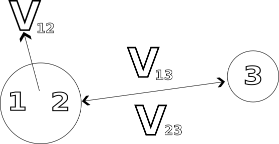
Figure 2: Visualization of the $e^{-itH_{a}}$ flow for $a=(12)(3)$

∎

2.2 Ruelle’s Theorem in the Context of Fiber Space

In this section, we present a proof of Ruelle’s theorem in fiber space $\mathcal{L}^{2}(X_{v_{T}})$ is presented, utilizing self-adjointness and local compactness, which are the two essential components of the proof of Ruelle’s theorem (see e.g., Theorem 2.4 in [HS1]). Ruelle’s theorem provides a characterization of all scattering states in $\mathcal{L}^{2}(X_{v_{T}})$.

We initiate our discussion with the self-adjointness of $H$. Define

$$\mathcal{D}(H):=\{f_{v_{T}}(x)\in\mathcal{L}^{2}(X_{v_{T}}):Hf_{v_{T}}\in\mathcal{L}^{2}(X_{v_{T}})\}.$$ (2.30)

For any given pair $f_{v_{T}},g_{v_{T}}\in\mathcal{D}(H)$, the following identity holds true:

$$(f_{v_{T}}(x),Hg_{v_{T}}(x))_{\mathcal{L}^{2}(X_{v_{T}})}=(\tilde{f}_{v_{T}}(x_{1}-x_{2},x_{2}),\tilde{H}(v_{T},3)\tilde{g}_{v_{T}}(x_{1}-x_{2},x_{2}))_{\mathcal{L}^{2}_{x_{1},x_{2}}(\mathbb{R}^{6})}.$$ (2.31)

Here,

$$\tilde{H}_{0}(v_{T},3):=\omega_{1}(P_{1})+\omega_{2}(P_{2})+\omega_{3}(v_{T}-P_{1}-P_{2}),$$ (2.32)

and

$$\tilde{V}_{3}(x_{1},x_{2}):=V_{12}(x_{1}-x_{2})+V_{13}(x_{1})+V_{23}(x_{2}),\leavevmode\nobreak\ \text{ and }\tilde{H}(v_{T},3):=\tilde{H}_{0}(v_{T})+\tilde{V}_{3}(x_{1},x_{2}).$$ (2.33)

Lemma 2.3.

(2.31) is true.

Proof.

First of all, we have the following identity:

$$H= e^{-ix_{3}\cdot P_{1}}e^{-ix_{3}\cdot P_{2}}(\omega_{1}(P_{1})+\omega_{2}(P_{2})+\omega_{3}(P_{3}-P_{2}-P_{1})+\tilde{V}(x_{1},x_{2}))e^{ix_{3}\cdot P_{1}}e^{ix_{3}\cdot P_{2}}$$

$$= e^{-ix_{3}\cdot P_{1}}e^{-ix_{3}\cdot P_{2}}\tilde{H}(P_{3},3)e^{ix_{3}\cdot P_{1}}e^{ix_{3}\cdot P_{2}}.$$ (2.34)

Employing the convention from (2.8), it’s evident that for all $f_{v_{T}}\in\mathcal{L}^{2}(X_{v_{T}})$,

$$\tilde{f}_{v_{T}}(x_{1}-x_{2},x_{2})=e^{-iv_{T}\cdot x_{3}}e^{ix_{3}\cdot P_{1}}e^{ix_{3}\cdot P_{2}}f_{v_{T}}(x).$$ (2.35)

Furthermore, based on (2.12), we can deduce:

$$(f_{v_{T}}(x),g_{v_{T}}(x))_{\mathcal{L}^{2}(X_{v_{T}})}= \int d^{3}y_{1}d^{3}y_{2}(\tilde{f}_{v_{T}}(y_{1},y_{2}))^{*}\tilde{g}_{v_{T}}(y_{1},y_{2})$$

$$(\text{take }y_{1}=x_{1}-x_{2},y_{2}=x_{2})= \int d^{3}x_{1}d^{3}x_{2}(\tilde{f}_{v_{T}}(x_{1}-x_{2},x_{2}))^{*}\tilde{g}_{v_{T}}(x_{1}-x_{2},x_{2}).$$ (2.36)

According to (2.34), (2.35) and (2.36), their inner product can be expressed as follows:

$$(f_{v_{T}}(x),Hg_{v_{T}}(x))_{\mathcal{L}^{2}(X_{v_{T}})}$$ (2.37)

$$= (\tilde{f}_{v_{T}}(x_{1}-x_{2},x_{2}),\widetilde{Hg}_{v_{T}}(x_{1}-x_{2},x_{2}))_{\mathcal{L}^{2}_{x_{1},x_{2}}(\mathbb{R}^{6})}$$ (2.38)

$$= (\tilde{f}_{v_{T}}(x_{1}-x_{2},x_{2})e^{iv_{T}\cdot x_{3}},e^{-iv_{T}\cdot x_{3}}e^{ix_{3}\cdot P_{1}}e^{ix_{3}\cdot P_{2}}Hg_{v_{T}}(x))_{\mathcal{L}^{2}_{x_{1},x_{2}}(\mathbb{R}^{6})}$$ (2.39)

$$= (\tilde{f}_{v_{T}}(x_{1}-x_{2},x_{2})e^{iv_{T}\cdot x_{3}},\tilde{H}(v_{T},3)e^{-iv_{T}\cdot x_{3}}e^{ix_{3}\cdot P_{1}}e^{ix_{3}\cdot P_{2}}g_{v_{T}}(x))_{\mathcal{L}^{2}_{x_{1},x_{2}}(\mathbb{R}^{6})}$$ (2.40)

$$= (\tilde{f}_{v_{T}}(x_{1}-x_{2},x_{2}),\tilde{H}(v_{T},3)\tilde{g}_{v_{T}}(x_{1}-x_{2},x_{2}))_{\mathcal{L}^{2}_{x_{1},x_{2}}(\mathbb{R}^{6})}.$$ (2.41)

∎

Lemma 2.3 implies that the self-adjointness of $H$ on $\mathcal{D}(H)$ corresponds to the self-adjointness of $\tilde{H}(v_{T},3)$ on $\mathcal{D}(\tilde{H}(v_{T},3)):=\{f(x_{1},x_{2})\in\mathcal{L}^{2}(\mathbb{R}^{6}):\tilde{H}(v_{T},3)f\in\mathcal{L}^{2}(\mathbb{R}^{6})\}$, which has been well established in literature (see e.g. page 20 in [CL2002] or [RS4]). Consequently, $H$ is self-adjoint on $\mathcal{D}(H)$. Recall that $\tilde{x}=(x_{1}-x_{2},x_{2}-x_{3},x_{3}-x_{1})\in\mathbb{R}^{9}$.

Lemma 2.4 (Local compactness property).

Let $f(x):=\tilde{f}(x_{1}-x_{2},x_{2}-x_{3})\in\mathcal{L}^{\infty}_{x}(\mathbb{R}^{9})$ with

$$f(x)=\tilde{f}(x_{1}-x_{2},x_{2}-x_{3})\to 0$$ (2.42)

as $|\tilde{x}|\to\infty$. Under Assumption 1.4 part (a), the operator

$$f(x)(z-H)^{-1}\text{ is compact on }\mathcal{L}^{2}(X_{v_{T}})$$ (2.43)

for any $z$ in the resolvent set $\rho(H)$. We refer to this by saying that $H$ has the local compactness property.

Proof.

Here, $|\tilde{x}|$ is equivalent to $|x_{1}-x_{2}|+|x_{1}-x_{3}|$ because

$$|x_{1}-x_{2}|+|x_{2}-x_{3}|\lesssim\sqrt{|x_{1}-x_{2}|^{2}+|x_{1}-x_{3}|^{2}+|x_{2}-x_{3}|^{2}}$$ (2.44)

and

$$\sqrt{|x_{1}-x_{2}|^{2}+|x_{1}-x_{3}|^{2}+|x_{2}-x_{3}|^{2}}\lesssim |x_{1}-x_{2}|+|x_{1}-x_{3}|+|x_{2}-x_{3}|$$

$$\lesssim |x_{1}-x_{2}|+|x_{2}-x_{3}|$$ (2.45)

by using triangle inequality. Let $g_{v_{T}}\in\mathcal{L}^{2}(X_{v_{T}})$. Based on the definition of $\mathcal{L}^{2}(X_{v_{T}})$, we have $f(x)(H-z)^{-1}g_{v_{T}}\in\mathcal{L}^{2}(X_{v_{T}})$. We rewrite $f(x)(H-z)^{-1}g_{v_{T}}$ as

$$f(x)(H-z)^{-1}g_{v_{T}}=e^{-ix_{3}\cdot P_{1}}e^{-ix_{3}\cdot P_{2}}\tilde{f}(x_{1},x_{2})(\tilde{H}(v_{T},3)-z)^{-1}\tilde{g}_{v_{T}}(x_{1},x_{2})e^{iv_{T}\cdot x_{3}}.$$ (2.46)

Using the second resolvent identity, we obtain

$$\tilde{f}(x_{1},x_{2})(\tilde{H}(v_{T},3)-z)^{-1}= \tilde{f}(x_{1},x_{2})(\tilde{H}_{0}(v_{T},3)-z)^{-1}$$

$$-\tilde{f}(x_{1},x_{2})(\tilde{H}_{0}(v_{T},3)-z)^{-1}\tilde{V}_{3}(x_{1},x_{2})(\tilde{H}(v_{T},3)-z)^{-1}.$$ (2.47)

The compactness of $\tilde{f}(x_{1},x_{2})(\tilde{H}_{0}(v_{T},3)-z)^{-1}$ on $\mathcal{L}^{2}_{x_{1},x_{2}}(\mathbb{R}^{6})$ is due to Assumption 1.4 part (a) and (2.42). By utilizing (2.47) and the compactness of $\tilde{f}(x_{1},x_{2})(\tilde{H}_{0}(v_{T},3)-z)^{-1}$ on $\mathcal{L}^{2}_{x_{1},x_{2}}(\mathbb{R}^{6})$, we can conclude that $f(x)(\tilde{H}(v_{T},3)-z)^{-1}$ is also compact on $\mathcal{L}^{2}(X_{v_{T}})$. Using (2.46) and the compactness of $f(x)(\tilde{H}(v_{T},3)-z)^{-1}$ on $\mathcal{L}^{2}(X_{v_{T}})$, we can further conclude that $f(x)(H-z)^{-1}$ is also compact on $\mathcal{L}^{2}(X_{v_{T}})$. ∎

Lemma 2.5 (Ruelle’s theorem in fiber space).

Suppose that $H=H^{*}$ on $\mathcal{D}(H)$ has the local compactness property. Let $\mathcal{H}_{B}=\mathcal{H}_{B}(v_{T})$ be the subspace spanned by all eigenvectors of $H$, and $\mathcal{H}_{C}=\mathcal{H}_{C}(v_{T})=\mathcal{H}_{B}^{\perp}$. If $\chi_{R}(\tilde{x})$ is the characteristic function of some ball $|\tilde{x}|<R$, then

$$\varphi\in\mathcal{H}_{B}\iff\lim\limits_{R\to\infty}\|(1-\chi_{R})e^{\pm itH}\varphi\|_{\mathcal{L}^{2}(X_{v_{T}})}=0\text{ uniformly in }0\leq t<\infty;$$ (2.48)

$$\psi\in\mathcal{H}_{C}\iff\lim\limits_{t\to\infty}t^{-1}\int_{0}^{t}ds\|\chi_{R}e^{\pm isH}\psi\|_{\mathcal{L}^{2}(X_{v_{T}})}^{2}=0\quad\text{ for any }R<\infty.$$ (2.49)

In particular, there exists a sequence of time $\{t_{n}\}_{n=1}^{n=\infty}$, with $t_{n}=t_{n}(\psi,R)\uparrow\infty$ as $n\to\infty$, such that

$$\|\chi_{R}e^{-it_{n}H}P_{c}\psi\|_{\mathcal{L}^{2}(X_{v_{T}})}<1/n,\quad\text{ for all }n\in\mathbb{N},$$ (2.50)

where $P_{c}=P_{c}(v_{T})$ denotes the projection on $\mathcal{H}_{C}$.

Proof.

See the proof of Theorem 2.4 in [HS1]. ∎

By applying Ruelle’s theorem in $\mathcal{L}^{2}(X_{v_{T}})$, we obtain a precise definition of $P_{c}(v_{T})$, which is the projection onto the space of all scattering states in $\mathcal{L}^{2}(X_{v_{T}})$.

2.3 Ruelle’s theorem in the full space and the scattering projection

In this section, we demonstrate how to prove Ruelle’s theorem in $\mathcal{L}^{2}_{x}(\mathbb{R}^{9})$ by utilizing Ruelle’s theorem in fiber space $\mathcal{L}^{2}(X_{v_{T}})$ as described in Lemma 2.5. Let $\psi\in C^{\infty}_{0}(\mathbb{R}^{9})$. We can write $\psi$ as

$$\psi(x_{1},x_{2},x_{3})=e^{-ix_{3}\cdot P_{1}}e^{-ix_{3}\cdot P_{2}}\psi(x_{1}+x_{3},x_{2}+x_{3},x_{3}).$$ (2.51)

Define $\tilde{\psi}(x_{1},x_{2},x_{3}):=\psi(x_{1}+x_{3},x_{2}+x_{3},x_{3})$. Then $\tilde{\psi}\in\mathcal{L}^{2}_{x}(\mathbb{R}^{9})$ and for any $t\in\mathbb{R}$, we have

$$e^{-itH}\psi=\frac{1}{(2\pi)^{3/2}}e^{-ix_{3}\cdot P_{1}}e^{-ix_{3}\cdot P_{2}}\int d^{3}q_{3}e^{-it\tilde{H}(q_{3},3)}\tilde{\psi}(x_{1},x_{2},\hat{q}_{3}),$$ (2.52)

where $\tilde{\psi}(x_{1},x_{2},\hat{q}_{3})$ denotes the Fourier transform in $x_{3}$ variable

$$\tilde{\psi}(x_{1},x_{2},\hat{q}_{3}):=\mathscr{F}_{x_{3}}[\tilde{\psi}](q_{3})=\frac{1}{(2\pi)^{3/2}}\int d^{3}x_{3}e^{-iq_{3}\cdot x_{3}}\tilde{\psi}(x_{1},x_{2},x_{3})$$ (2.53)

and by using Fourier inversion theorem, we have

$$\tilde{\psi}(x)=\mathscr{F}_{q_{3}}^{-1}[\tilde{\psi}](x_{3})=\frac{1}{(2\pi)^{3/2}}\int d^{3}q_{3}e^{iq_{3}\cdot x_{3}}\tilde{\psi}(x_{1},x_{2},\hat{q}_{3}).$$ (2.54)

Here, for $\tilde{H}(q_{3},3)$, see (2.32) and (2.33). $\psi$ has following orthogonal decomposition

$$\psi=\psi_{sc}+\psi_{bs}$$ (2.55)

where

$$\psi_{sc}(x):= P_{c}(P_{1}+P_{2}+P_{3})e^{-ix_{3}\cdot P_{1}}e^{-ix_{3}\cdot P_{2}}\tilde{\psi}(x)$$

$$= e^{-ix_{3}\cdot P_{1}}e^{-ix_{3}\cdot P_{2}}P_{c}(P_{3})\tilde{\psi}(x)$$ (2.56)

and

$$\psi_{bs}(x):= (1-P_{c}(P_{1}+P_{2}+P_{3}))e^{-ix_{3}\cdot P_{1}}e^{-ix_{3}\cdot P_{2}}\tilde{\psi}(x)$$

$$= e^{-ix_{3}\cdot P_{1}}e^{-ix_{3}\cdot P_{2}}(1-P_{c}(P_{3}))\tilde{\psi}(x).$$ (2.57)

We use $P_{c}(P_{1}+P_{2}+P_{3})$ here because $P_{1}+P_{2}+P_{3}$ is really the total quasi-momentum of three particles. Here, we also use

$$P_{c}(P_{1}+P_{2}+P_{3})e^{-ix_{3}\cdot P_{1}}e^{-ix_{3}\cdot P_{2}}=e^{-ix_{3}\cdot P_{1}}e^{-ix_{3}\cdot P_{2}}P_{c}(P_{3}),$$ (2.58)

where $P_{c}(P_{3})$ on $\mathcal{L}^{2}_{x}(\mathbb{R}^{9})$ is understood as

$$P_{c}(P_{3})f=\frac{1}{(2\pi)^{3/2}}\int d^{3}q_{3}e^{ix_{3}\cdot q_{3}}P_{c}(q_{3})f(x_{1},x_{2},\hat{q}_{3}),\quad f\in\mathcal{L}^{2}_{x}(\mathbb{R}^{9}),$$ (2.59)

and $P_{c}(q_{3})$ is defined in Lemma 2.5 for all $q_{3}\in\mathbb{R}^{3}$ by taking $H=\tilde{H}(q_{3},3)$. Given the equivalence between $\tilde{H}(P_{3},3)$ and our three-body Hamiltonian $H$ on $\mathcal{L}^{2}_{x}(\mathbb{R}^{9})$, we define $P_{sc}$ as the projection onto the space of all scattering states of $H$:

$$P_{sc}:=P_{c}(P_{1}+P_{2}+P_{3}).$$ (2.60)

We also define $P_{bs}$ as the projection onto the spac eof all bound states of $H$:

$$P_{bs}:=1-P_{sc}.$$ (2.61)

Consequently, we can represent the scattering component of $\psi$ as

$$\psi_{sc}=P_{sc}\psi,$$ (2.62)

and the non-scattering component of $\psi$ as

$$\psi_{bs}=P_{bs}\psi.$$ (2.63)

Note that $\psi_{sc}(x)$ is orthogonal to $\psi_{bs}(x)$ in $\mathcal{L}^{2}_{x}(\mathbb{R}^{9})$ due to Plancherel’s theorem: for some constant $c>0$, we have

$$(\psi_{sc}(x),\psi_{bs}(x))_{\mathcal{L}^{2}_{x}(\mathbb{R}^{9})}= (\tilde{\psi}_{sc}(x),\tilde{\psi}_{bs}(x))_{\mathcal{L}^{2}_{x}(\mathbb{R}^{9})}$$

$$= c\int d^{3}q_{3}(P_{c}(q_{3})\tilde{\psi}_{sc}(x_{1},x_{2},\hat{q}_{3}),(1-P_{c}(q_{3}))\tilde{\psi}_{bs}(x_{1},x_{2},\hat{q}_{3}))_{\mathcal{L}^{2}_{x_{1},x_{2}}(\mathbb{R}^{6})}$$

$$= 0.$$ (2.64)

We can apply the same orthogonal decomposition to all $\psi\in\mathcal{L}^{2}_{x}(\mathbb{R}^{9})$ by using the density of $C_{0}^{\infty}(\mathbb{R}^{9})$ in $\mathcal{L}^{2}_{x}(\mathbb{R}^{9})$:

Proposition 2.1.

For all $\psi\in\mathcal{L}^{2}_{x}(\mathbb{R}^{9})$, $\psi$ has an orthogonal decomposition

$$\psi(x)=\psi_{sc}(x)+\psi_{bs}(x)$$ (2.65)

where $\psi_{sc}$ and $\psi_{bs}$ are defined in (2.62) and (2.63), respectively.

In the following, we provide a proof of Ruelle’s theorem in $\mathcal{L}^{2}_{x}(\mathbb{R}^{9})$ space:

Proposition 2.2 (Ruelle’s theorem in $\mathcal{L}^{2}_{x}(\mathbb{R}^{9})$).

If Assumptions (1.1) and 1.4 part (a) hold, and if $\chi_{R}(\tilde{x})$ is the characteristic function of some ball $|\tilde{x}|<R$, then for all $\psi\in\mathcal{L}^{2}_{x}(\mathbb{R}^{9})$,

$$\lim\limits_{R\to\infty}\|(1-\chi_{R})e^{\pm itH}\psi_{bs}\|_{\mathcal{L}^{2}_{x}(\mathbb{R}^{9})}=0\text{ uniformly in }0\leq t<\infty;$$ (2.66)

$$\lim\limits_{t\to\infty}t^{-1}\int_{0}^{t}ds\|\chi_{R}e^{\pm isH}\psi_{sc}\|_{\mathcal{L}^{2}_{x}(\mathbb{R}^{9})}^{2}=0\quad\text{ for any }R<\infty.$$ (2.67)

In particular, there exists a sequence of time $\{t_{n}\}_{n=1}^{n=\infty}$, with $t_{n}=t_{n}(\psi,R)\uparrow\infty$ as $n\to\infty$, such that

$$\|\chi_{R}e^{-it_{n}H}\psi_{sc}\|_{\mathcal{L}^{2}(\mathbb{R}^{9})}<1/n,\quad\text{ for all }n\in\mathbb{N}.$$ (2.68)

Proof.

Choose $\psi\in\mathcal{L}^{2}_{x}(\mathbb{R}^{9})$. For any $\epsilon>0$, there exists $\psi_{\epsilon}\in C^{\infty}_{0}(\mathbb{R}^{9})$ such that $\|\psi-\psi_{\epsilon}\|_{\mathcal{L}^{2}_{x}(\mathbb{R}^{9})}<\epsilon$. Our goal is to show that

$$\limsup\limits_{R\to\infty}\|(1-\chi_{R})e^{\pm itH}[\psi_{\epsilon}]_{bs}\|_{\mathcal{L}^{2}_{x}(\mathbb{R}^{9})}=0\quad\text{ uniformly in }0\leq t<\infty$$ (2.69)

and

$$\limsup\limits_{t\to\infty}t^{-1}\int_{0}^{t}ds\|\chi_{R}e^{\pm isH}[\psi_{\epsilon}]_{sc}\|_{\mathcal{L}^{2}_{x}(\mathbb{R}^{9})}^{2}=0\quad\text{ for any }R<\infty,$$ (2.70)

where $\psi_{\epsilon}=[\psi_{\epsilon}]_{sc}+[\psi_{\epsilon}]_{bs}$ with $[\psi_{\epsilon}]_{sc}$ and $[\psi_{\epsilon}]_{bs}$ defined in (2.62) and (2.63), respectively, by substituting $\psi$ with $\psi_{\epsilon}$. Once we establish (2.69) and (2.70), we can obtain the following inequalities for any $\epsilon>0$:

$$\limsup\limits_{R\to\infty}\|(1-\chi_{R})e^{\pm itH}\psi_{bs}\|_{\mathcal{L}^{2}_{x}(\mathbb{R}^{9})}<\epsilon\text{ uniformly in }0\leq t<\infty$$ (2.71)

and

$$\limsup\limits_{t\to\infty}t^{-1}\int_{0}^{t}ds\|\chi_{R}e^{\pm isH}\psi_{sc}\|_{\mathcal{L}^{2}_{x}(\mathbb{R}^{9})}^{2}<\epsilon^{2}\quad\text{ for any }R<\infty,$$ (2.72)

since due to unitarity of $e^{-itH}$ on $\mathcal{L}^{2}_{x}(\mathbb{R}^{9})$, we have

$$\begin{split}t^{-1}\int_{0}^{t}ds\|\chi_{R}e^{\pm isH}(\psi_{sc}-[\psi_{\epsilon}]_{sc})\|_{\mathcal{L}^{2}_{x}(\mathbb{R}^{9})}^{2}\leq&\|\psi_{sc}-[\psi_{\epsilon}]_{sc}\|_{\mathcal{L}^{2}_{x}(\mathbb{R}^{9})}^{2}\\ =&\|P_{c}(P_{1}+P_{2}+P_{3})(\psi-\psi_{\epsilon})\|_{\mathcal{L}^{2}_{x}(\mathbb{R}^{9})}^{2}\\ \leq&\|\psi-\psi_{\epsilon}\|_{\mathcal{L}^{2}_{x}(\mathbb{R}^{9})}^{2}\end{split}$$ (2.73)

and

$$\begin{split}\|(1-\chi_{R})e^{\pm itH}(\psi_{bs}-[\psi_{\epsilon}]_{bs})\|_{\mathcal{L}^{2}_{x}(\mathbb{R}^{9})}\leq&\|\psi_{bs}-[\psi_{\epsilon}]_{bs}\|_{\mathcal{L}^{2}_{x}(\mathbb{R}^{9})}\\ =&\|(1-P_{c}(P_{1}+P_{2}+P_{3}))(\psi-\psi_{\epsilon})\|_{\mathcal{L}^{2}_{x}(\mathbb{R}^{9})}\\ \leq&\|\psi-\psi_{\epsilon}\|_{\mathcal{L}^{2}_{x}(\mathbb{R}^{9})}.\end{split}$$ (2.74)

Therefore, we conclude (2.66) and (2.67). Now let us prove (2.69) and (2.70). Let us define

$$\tilde{\chi}_{R}(x_{1},x_{2}):= e^{ix_{3}\cdot P_{2}}e^{ix_{3}\cdot P_{1}}\chi_{R}(\tilde{x})e^{-ix_{3}\cdot P_{1}}e^{-ix_{3}\cdot P_{2}}$$

$$= e^{ix_{3}\cdot P_{2}}e^{ix_{3}\cdot P_{1}}\chi_{R}(x_{1}-x_{2},x_{2}-x_{3},x_{3}-x_{1})e^{-ix_{3}\cdot P_{1}}e^{-ix_{3}\cdot P_{2}}$$

$$= \chi_{R}(x_{1}-x_{2},x_{2},-x_{1}),$$ (2.75)

$$\tilde{\psi}_{\epsilon}=e^{ix_{3}\cdot P_{2}}e^{ix_{3}\cdot P_{1}}\psi_{\epsilon},$$ (2.76)

$$[\tilde{\psi}_{\epsilon}]_{sc}:=P_{c}(P_{3})\tilde{\psi}_{\epsilon}$$ (2.77)

and

$$[\tilde{\psi}_{\epsilon}]_{bs}:=(1-P_{c}(P_{3}))\tilde{\psi}_{\epsilon}.$$ (2.78)

Since $\psi_{\epsilon}\in C_{0}^{\infty}(\mathbb{R}^{9})$, it follows that $\tilde{\psi}_{\epsilon}(x_{1},x_{2},\hat{q}_{3})\in\mathcal{L}^{2}_{x_{1},x_{2}}(\mathbb{R}^{6})$ for all $q_{3}\in\mathbb{R}^{3}$. Hence, we have

$$e^{-ix_{3}\cdot P_{1}}e^{-ix_{3}\cdot P_{2}}\tilde{\psi}_{\epsilon}(x_{1},x_{2},\hat{q}_{3})e^{ix_{3}\cdot q_{3}}=\tilde{\psi}_{\epsilon}(x_{1}-x_{3},x_{2}-x_{3})e^{ix_{3}\cdot q_{3}}\in\mathcal{L}^{2}(X_{q_{3}}),$$ (2.79)

since, by taking

$$\bar{\psi}_{\epsilon}(y_{1},y_{2})=\tilde{\psi}_{\epsilon}(y_{1}+y_{2},y_{2}),$$ (2.80)

we have $\tilde{\psi}_{\epsilon}(x_{1}-x_{3},x_{2}-x_{3})=\bar{\psi}_{\epsilon}(x_{1}-x_{2},x_{2}-x_{3})\in\mathcal{L}^{2}_{y_{1},y_{2}}(\mathbb{R}^{6})$ satisfying

$$\|\tilde{\psi}_{\epsilon}(y_{1},y_{2})\|_{\mathcal{L}^{2}_{y_{1},y_{2}}(\mathbb{R}^{6})}=\|\bar{\psi}_{\epsilon}(y_{1},y_{2})\|_{\mathcal{L}^{2}_{y_{1},y_{2}}(\mathbb{R}^{6})}.$$

Using Assumptions 1.1 and 1.2 part (b), we conclude that for all $q_{k}\in\mathbb{R}^{3}$, $\tilde{H}(q_{k},3)$ is self-adjoint and has local compactness. Given the self-adjointness and local compactness of $\tilde{H}(q_{k},3)$, the conclusion of Lemma 2.5 is valid for $\tilde{H}(q_{k},3)$. Therefore, we have that for all $q_{3}\in\mathbb{R}^{3}$ by applying (2.76), (2.8) and (2.13),

$$\begin{split}&\lim\limits_{R\to\infty}\|(1-\chi_{R})e^{\pm itH}[\psi_{\epsilon}]_{bs}\|_{\mathcal{L}^{2}(X_{q_{3}})}\\ =&\lim\limits_{R\to\infty}\|(1-\chi_{R})e^{\pm itH}e^{-ix_{3}\cdot P_{1}}e^{-ix_{3}\cdot P_{2}}[\tilde{\psi}_{\epsilon}]_{bs}(x_{1},x_{2},\hat{q}_{3})e^{ix_{3}\cdot q_{3}}\|_{\mathcal{L}^{2}(X_{q_{3}})}\\ =&\lim\limits_{R\to\infty}\|(1-\chi_{R})e^{-ix_{3}\cdot P_{1}}e^{-ix_{3}\cdot P_{2}}e^{\pm it\tilde{H}(P_{3},3)}[\tilde{\psi}_{\epsilon}]_{bs}(x_{1},x_{2},\hat{q}_{3})e^{ix_{3}\cdot q_{3}}\|_{\mathcal{L}^{2}(X_{q_{3}})}\\ =&\lim\limits_{R\to\infty}\|(1-\tilde{\chi}_{R}(x_{1},x_{2}))e^{\pm it\tilde{H}(q_{3},3)}[\tilde{\psi}_{\epsilon}]_{bs}(x_{1},x_{2},\hat{q}_{3})\|_{\mathcal{L}^{2}_{x_{1},x_{2}}(\mathbb{R}^{6})}\\ =&0\end{split}$$ (2.81)

uniformly in $0\leq t<\infty$, and

$$\begin{split}&\lim\limits_{t\to\infty}t^{-1}\int_{0}^{t}ds\|\chi_{R}e^{\pm itH}[\psi_{\epsilon}]_{sc}\|_{\mathcal{L}^{2}(X_{q_{3}})}\\ =&\lim\limits_{t\to\infty}t^{-1}\int_{0}^{t}ds\|\chi_{R}e^{\pm itH}e^{-ix_{3}\cdot P_{1}}e^{-ix_{3}\cdot P_{2}}[\tilde{\psi}_{\epsilon}]_{sc}(x_{1},x_{2},\hat{q}_{3})e^{ix_{3}\cdot q_{3}}\|_{\mathcal{L}^{2}(X_{q_{3}})}^{2}\\ =&\lim\limits_{t\to\infty}t^{-1}\int_{0}^{t}ds\|\chi_{R}e^{-ix_{3}\cdot P_{1}}e^{-ix_{3}\cdot P_{2}}e^{\pm it\tilde{H}(P_{3},3)}[\tilde{\psi}_{\epsilon}]_{sc}(x_{1},x_{2},\hat{q}_{3})e^{ix_{3}\cdot q_{3}}\|_{\mathcal{L}^{2}(X_{q_{3}})}^{2}\\ =&\lim\limits_{t\to\infty}t^{-1}\int_{0}^{t}ds\|\tilde{\chi}_{R}e^{\pm is\tilde{H}(q_{3},3)}[\tilde{\psi}_{\epsilon}]_{sc}(x_{1},x_{2},\hat{q}_{3})e^{ix_{3}\cdot q_{3}}\|_{\mathcal{L}^{2}_{x_{1},x_{2}}(\mathbb{R}^{6})}^{2}\\ =&0\end{split}$$ (2.82)

for any $R<\infty$. Set

$$a_{R}(q_{3},t):=\|(1-\chi_{R})e^{\pm itH}[\psi_{\epsilon}]_{bs}\|_{\mathcal{L}^{2}(X_{q_{3}})}$$ (2.83)

and

$$b_{t}(q_{3},R):=t^{-1}\int_{0}^{t}ds\|\chi_{R}e^{\pm itH}[\psi_{\epsilon}]_{sc}\|_{\mathcal{L}^{2}(X_{q_{3}})}^{2}.$$ (2.84)

Then $\lim\limits_{R\to\infty}a_{R}(q_{3},t)=0$ for all $q_{3}\in\mathbb{R}^{3},t\geq 0$, and $\lim\limits_{t\to\infty}b_{t}(q_{3},R)=0$ for all $q_{3}\in\mathbb{R}^{3},R\geq 0$. Hence, for all $q_{3}\in\mathbb{R}^{3},t\geq 0$,

$$|a_{R}(q_{3},t)|^{2}\to 0\quad\text{ as }R\to\infty$$ (2.85)

and

$$|a_{R}(q_{3},t)|^{2}\leq\|\tilde{\psi}_{\epsilon}(x_{1},x_{2},\hat{q}_{3})\|_{\mathcal{L}^{2}_{x_{1},x_{2}}(\mathbb{R}^{6})}^{2}\in\mathcal{L}^{1}_{q_{3}}(\mathbb{R}^{3}).$$ (2.86)

Therefore, due to Plancherel Theorem and Dominated Convergence Theorem, we obtain that for all $t\geq 0$,

$$\begin{split}&\|(1-\chi_{R})e^{\pm itH}(1-P_{c}(P_{1}+P_{2}+P_{3}))\psi_{\epsilon}\|_{\mathcal{L}^{2}_{x}(\mathbb{R}^{9})}\\ =&\|(1-\tilde{\chi}_{R})e^{\pm it\tilde{H}(P_{3},3)}(1-P_{c}(P_{3}))\tilde{\psi}_{\epsilon}\|_{\mathcal{L}^{2}_{x}(\mathbb{R}^{9})}\\ =&c\|\|(1-\tilde{\chi}_{R})e^{\pm it\tilde{H}(q_{3},3)}(1-P_{c}(q_{3}))\tilde{\psi}_{\epsilon}(x_{1},x_{2},\hat{q}_{3})\|_{\mathcal{L}^{2}_{x_{1},x_{2}}(\mathbb{R}^{6})}\|_{\mathcal{L}^{2}_{q_{3}}(\mathbb{R}^{3})}\\ =&c\|a_{R}(q_{3},t)\|_{\mathcal{L}^{2}_{q_{3}}(\mathbb{R}^{3})}\\ \to&0\end{split}$$ (2.87)

as $R\to\infty$. Therefore, we obtain (2.69). Similarly, since for all $q_{3}\in\mathbb{R}^{3},R\geq 0$,

$$b_{t}(q_{3},R)\to 0\quad\text{ as }t\to\infty$$ (2.88)

and

$$|b_{t}(q_{3},R)|\leq\|\tilde{\psi}_{\epsilon}(x_{1},x_{2},\hat{q}_{3})\|_{\mathcal{L}^{2}_{x_{1},x_{2}}(\mathbb{R}^{6})}^{2}\in\mathcal{L}^{1}_{q_{3}}(\mathbb{R}^{3}),$$ (2.89)

by utilizing the Plancherel Theorem, Fubini’s Theorem, and Dominated Convergence Theorem, we have that for all $R\geq 0$,

$$\begin{split}&t^{-1}\int_{0}^{t}ds\|\chi_{R}e^{\pm isH}P_{c}(P_{1}+P_{2}+P_{3})\psi\|_{\mathcal{L}^{2}_{x}(\mathbb{R}^{9})}^{2}\\ =&t^{-1}\int_{0}^{t}ds\|\tilde{\chi}_{R}e^{\pm is\tilde{H}(P_{3},3)}P_{c}(P_{3})\psi_{\epsilon}\|_{\mathcal{L}^{2}_{x}(\mathbb{R}^{9})}^{2}\\ =&ct^{-1}\int_{0}^{t}ds\|\|\tilde{\chi}_{R}e^{\pm is\tilde{H}(q_{3},3)}P_{c}(q_{3})\psi_{\epsilon}(x_{1},x_{2},\hat{q}_{3})\|_{\mathcal{L}^{2}_{x_{1},x_{2}}(\mathbb{R}^{6})}\|_{\mathcal{L}^{2}_{q_{3}}(\mathbb{R}^{3})}^{2}\\ =&c\int d^{3}q_{3}b_{t}(q_{3},R)\\ \to&0\end{split}$$ (2.90)

as $t\to\infty$, where $c$ is a positive constant. Therefore, we obtain (2.70). We finish the proof. ∎

2.4 Threshold and Feynman-Hellmann Theorem

In this section, we will introduce the concept of a threshold point in a two/three-body Hamiltonian and discuss the utilization of the Feynman-Hellmann Theorem. Generally speaking, when the spectrum of a Hamiltonian H is near the threshold points, the dispersive behavior of the operator $e^{-itH}$ is abnormal. The Feynman-Hellmann Theorem provides us with a continuity property for these threshold points.

2.4.1 The Threshold set of one/two-body Hamiltonians

For a threshold point of a Hamiltonian, a similar notion exists in the case of a one-body Schrödinger operator, $H=-\Delta_{x}+V(x)$, where, for example, $\langle x\rangle^{\sigma}V(x)\in\mathcal{L}^{\infty}_{x}(\mathbb{R}^{n})$ holds for some $\sigma>3$. $0$ is considered as a threshold point. This notion for Schrödinger operators comes from the observation that when the spectrum of $H$ is near $0$, the dispersive estimate of $e^{itH}$ exhibits abnormal behavior due to the possible presence of the zero eigenvalue, the zero resonance for $H$ or both, which can be considered as an exceptional event. See, for example, [JK1979], which provides a detailed explanation of the zero threshold point for Schrödinger operators. Here, we refer to $f$ as a resonance of a one-body Schrödinger operator $H=-\Delta_{x}+V(x)$ if $f$ is the distributional solution to $H\psi(x)=0$ with $f\notin\mathcal{L}^{2}_{x}(\mathbb{R}^{3})$ while $\langle x\rangle^{-\sigma}f\in\mathcal{L}^{2}_{x}(\mathbb{R}^{3})$ for some $\sigma>1/2$. See, for example, [JK1979] for the concept of resonance. In the case of free Schrödinger evolution, the following relationship holds:

$$\|e^{-it(-\Delta_{x})}\|_{\mathcal{L}^{1}_{x}(\mathbb{R}^{3})\to\mathcal{L}^{\infty}_{x}(\mathbb{R}^{3})}\lesssim\frac{1}{|t|^{3/2}}.$$ (2.91)

However, when $e^{itH}$ behaves ”badly” around $0$ due to $0$ being either a resonance or an eigenvalue of $H$, we observe only a point-wise decay of $1/\sqrt{|t|}$: for some initial data $u_{0}(x)$, which decays sufficiently rapidly at infinity, the solution $u(t,x)=e^{-itH}u_{0}(x)$ admits as $t\to\infty$ an asymptotic expansion

$$u(t,x)=\sum\limits_{\text{finite}}a_{j}e^{i\lambda_{j}t}\phi_{j}(x)+\frac{1}{\sqrt{|t|}}B_{0}u_{0}(x)+\frac{1}{|t|^{3/2}}B_{1}u_{0}(x)+\cdots,$$ (2.92)

which is valid locally in space. Here $\phi_{j}(x)$ are eigenfunctions of $H$ with eigenvalues $\lambda_{j}$, and $B_{0}\neq 0$ if $0$ is a resonance or an eigenvalue of $H$. The $B_{j},j=0,1,\cdots$ are finite-rank operators. For more detailed information and additional references, please refer to [GJY2004] (page 233) and the relevant literature cited therein. $0$ holds a special significance for the Schrödinger operator due to the fact that the group velocity of $-\Delta_{x}$ is given by $2P:=2(-i)\nabla_{x}$, and $0$ corresponds to the energy where $2P=0$. In the context of general one-/two-body Hamiltonians, we define a threshold point in a similar way. In the case of a three-body Hamiltonian $H$, we define a point $\lambda\in\mathbb{R}$ as a threshold point if the behavior of $e^{-itH}$ becomes ”abnormal” when the spectrum of $H$ is in the vicinity of $\lambda$.

Let us start with the one/two-body case. The threshold points are defined based on the concepts of group velocity and relative group velocity of two particles. In quantum mechanics, velocity is characterized by the concept of group velocity.

Definition 4 (Group velocity of a particle).

Let $\omega_{j}\in C^{1}(\mathbb{R}^{3})$ for $j=1,2,3$. The group velocity of particle $j$ is defined as

$$v_{j}(P_{j}):=\nabla_{P_{j}}[\omega_{j}(P_{j})],\quad P_{j}:=-i\nabla_{x_{j}}.$$ (2.93)

Definition 5 (Relative group velocity of two particles).

The relative group velocity of particles $j$ and $l$ with $1\leq j<l\leq 3$ is defined as

$$v_{jl}(P_{j},P_{l}):=v_{j}(P_{j})-v_{l}(P_{l}),\quad P_{j}:=-i\nabla_{x_{j}},P_{l}:=-i\nabla_{x_{l}},$$ (2.94)

where $v_{j}$ and $v_{l}$ are the group velocities of particles $j$ and $l$, respectively.

Now let us look at the relationship between two-body Hamiltonians and one-body Hamiltonians. In this section, we assume that $(jkl)$ is a permutation of $(123)$ with $j<k$ fixed. Let $a=(jk)(l)\in L$. Recall that

$$H^{a}:=\omega_{j}(P_{j})+\omega_{k}(P_{k})+V_{jk}(x_{j}-x_{k})$$ (2.95)

represents a two-body Hamiltonian. We introduce the following definition:

$$H^{a}(\eta):=\omega_{j}(\eta-P_{k})+\omega_{k}(P_{k})+V_{jk}(-x_{k})\quad\text{ for }\eta\in\mathbb{R}^{3}.$$ (2.96)

We can observe the relationship between $H^{a}$ and $H^{a}(\eta)$ through the following identity:

$$H^{a}=e^{-ix_{j}\cdot P_{k}}H^{a}(P_{j})e^{ix_{j}\cdot P_{k}}.$$ (2.97)

In (2.97), the appearance of $P_{j}$ in $H^{a}(P_{j})$ on the right-hand side corresponds to the total quasi-momentum of particle $j$ and particle $k$, which is $P_{j}+P_{k}$ in $H^{a}$, since we have

$$P_{j}+P_{k}=e^{-ix_{j}\cdot P_{k}}P_{j}e^{ix_{j}\cdot P_{k}},$$ (2.98)

and

$$F(|P_{j}+P_{k}-v|\leq\epsilon)=e^{-ix_{j}\cdot P_{k}}F(|P_{j}-v|\leq\epsilon)e^{ix_{j}\cdot P_{k}},\quad\text{for all }v\in\mathbb{R}^{3},\epsilon>0.$$ (2.99)

Here $F$ denotes a smooth cut-off function. When studying the two-body problem, it is common to simplify it by reducing it to a one-body problem using equation (2.97). The notion of threshold points for a two-body Hamiltonian $H^{a}$ is established within the framework of fixing the total quasi-momentum. In other words, the total quasi-momentum needs to be fixed prior to discussing the concept of a threshold point for the two-body Hamiltonian $H^{a}$. Here is the definition of a threshold point for a one-body Hamiltonian $H^{a}(\eta)$, where $a=(jk)(l)\in L$ and $\eta\in\mathbb{R}^{3}$:

Definition 6 (Threshold points for $H^{a}(\eta)$).

Given $\eta\in\mathbb{R}^{3}$ and $a=(jk)(l)\in L$, a threshold point $\lambda^{a}(\eta)$ of $H^{a}(\eta)$ occurs if

$$\lambda^{a}(\eta)=\omega_{j}(\eta-q_{k})+\omega_{k}(q_{k})$$ (2.100)

with $q_{k}$ satisfying

$$\nabla_{p_{k}}[\omega_{j}(\eta-p_{k})+\omega_{k}(p_{k})]|_{p_{k}=q_{k}}=0.$$ (2.101)

Definition 7 (Threshold points for $H^{a}$).

Given $v\in\mathbb{R}^{3}$ and $a=(jk)(l)\in L$, a threshold point $\lambda^{a}(v)$ of $H^{a}$, with a total quasi-momentum $v$, occurs if $\lambda^{a}(v)$ is a threshold point of $H^{a}(v)$.

According to Definitions 6 and 7, the collection of threshold points of $H^{a}(v)$ (where $v\in\mathbb{R}^{3}$) is equal to the set of threshold points of $H^{a}$ with a fixed total quasi-momentum $v$. Let $\tau^{a}(v)$ denote the set of all threshold points for $H^{a}(v)$, where $v\in\mathbb{R}^{3}$.

The definition of a threshold point for a three-body Hamiltonian relies on the concept of a generic one-body Hamiltonian and the notion of eigenfunctions of a one-body Hamiltonian. Now, let us proceed by introducing the notion of a generic one-body Hamiltonian. Given $a=(jk)(l)\in L$ and $\eta\in\mathbb{R}^{3}$, we let

$$H^{a}_{0}(\eta):=\omega_{j}(\eta-P_{k})+\omega_{k}(P_{k}).$$ (2.102)

Definition 8 (Eigenfunctions/eigenvalues of a one-body Hamiltonian).

Given $a=(jk)(l)\in L$ with $j<k$ and $\eta\in\mathbb{R}^{3}$, $\lambda$ is an eigenvalue of $H^{a}(\eta)$ if

$$H^{a}(\eta)f(x_{k})=\lambda f(x_{k})$$ (2.103)

for some $f(x_{k})\in\mathcal{L}^{2}_{x_{k}}(\mathbb{R}^{3})$. We refer to $f(x_{k})$ satisfying (2.103) as an eigenfunction of $H^{a}(\eta)$ with an eigenvalue $\lambda$.

When it comes to the concepts of eigenvalues and eigenfunctions of a two-body Hamiltonian $H^{a}(a=(jk)(l)\in L)$, we have to fix the total quasi-momentum of the two particles, and then delve into these concepts:

Definition 9 (Eigenvalues of a two-body Hamiltonian).

Given $a=(jk)(l)\in L$ with $j<k$ and $v\in\mathbb{R}^{3}$, $\lambda$ is an eigenvalue of $H^{a}$ with a total quasi-momentum $v$ if $\lambda$ is an eigenvalue of $H^{a}(v)$. For an eigenvalue $\lambda$, $f(x_{k}-x_{j})$ is an corresponding eigenfunction of $H^{a}$ with a total quasi-momentum $v$ if

$$H^{a}(v)f(x_{k})=\lambda f(x_{k}).$$ (2.104)

It is known, for example, by using resolvent, that if all threshold points are neither an eigenvalue nor a resonance, for a Schrödinger-tpye one-body Hamiltonian, we have some nice results:

Proposition 2.3.

If all threshold points have neither an eigenvalue nor a resonance for a Schrödinger-type one-body Hamiltonian, then such Schrödinger-type one-body Hamiltonian enjoys: for example, when $H_{s}=-\Delta_{x_{k}}+W(x_{k})$ for some $\langle x_{k}\rangle^{\sigma}W(x_{k})\in\mathcal{L}^{\infty}_{x_{k}}(\mathbb{R}^{3})$ for some $\sigma\geq 3$,

• There are at most finitely many eigenfunctions and eigenvalues.

• All of eigenfunctions are localized in space: for all eigenfunctions of $H_{s}$, $f_{e}(x_{k})$, $f_{e}(x_{k})$ satisfy, at least,

  $$\|\langle x_{k}\rangle^{\sigma}f_{e}(x_{k})\|_{\mathcal{L}^{2}_{x_{k}}(\mathbb{R}^{3})}\lesssim_{\sigma,H_{s}}\|f_{e}(x_{k})\|_{\mathcal{L}^{2}_{x_{k}}(\mathbb{R}^{3})}.$$ (2.105)

• $e^{itH_{s}}$ satisfies $\mathcal{L}^{p}$ decay estimates:

  $$\|e^{itH_{s}}P_{c}(H_{s})f(x_{k})\|_{\mathcal{L}^{p}_{x_{k}}(\mathbb{R}^{3})}\lesssim_{p,H_{s}}\frac{1}{|t|^{3(\frac{1}{2}-\frac{1}{p})}}\|f(x_{k})\|_{\mathcal{L}^{p^{\prime}}_{x_{k}}(\mathbb{R}^{3})},$$ (2.106)

  for all $f(x_{k})\in\mathcal{L}^{p^{\prime}}_{x_{k}}(\mathbb{R}^{3})\cap\mathcal{L}^{2}_{x_{k}}(\mathbb{R}^{3})$ and all $p\in[2,\infty]$, where $P_{c}(H_{s})$ denotes the projection on the continuous spectrum of $H_{s}$ and

  $$\frac{1}{p}+\frac{1}{p^{\prime}}=1.$$

• $e^{itH_{s}}$ satisfies the local decay property: for all $f(x_{k})\in\mathcal{L}^{2}_{x_{k}}(\mathbb{R}^{3})$ and $\epsilon>0,$, for $\lambda non-threshold$

  $$\|\langle x_{k}\rangle^{-1-\epsilon}\frac{1}{H_{s}-\lambda\pm i0}f(x_{k})\|_{\mathcal{L}^{2}_{x_{k},\lambda}(\mathbb{R}^{3+1})}\lesssim_{\epsilon}\|f(x_{k})\|_{\mathcal{L}^{2}_{x_{k}}(\mathbb{R}^{3})}.$$ (2.107)

Assumption 1.8 ensures that all sub-Hamiltonians $H^{a}$ with $a=(jk)(l)\in L$ and $H_{0}$ share similar properties outlined in Proposition 2.3, provided that their energy is away from finitely many points in each fiber space. These points will be used to define threshold points for our three-body Hamiltonian $H$, which will be elaborated upon in section 2.4.2.

2.4.2 Feynman-Hellmann Theorem

The discussion of this part is based on the following assumption on Assumptions 1.1- 1.8. Based on Assumption 1.1 and Theorem XIII.6 on page 87 in [RS1978], it can be inferred that for every $a=(jk)(l)\in L,\eta\in\mathbb{R}^{3}$, the operator $H^{a}(\eta)$ has a finite number of eigenvalues at most, denoted as $\lambda_{1}\leq\cdots\leq\lambda_{m}$ (where $\lambda_{r},r=1,\cdots,m,$ may be identical to one another), with $m\leq N$ for some constant $N$ which is independent on $\eta\in\mathbb{R}^{3}$.

The Feynman-Hellmann Theorem elucidates how these eigenvalues change as $\eta\in\mathbb{R}^{3}$ varies. In simple terms, the Feynman-Hellmann Theorem supplies a formula for the derivative of the eigenvalues with respect to the parameter.

Theorem 2.2 (Feynman-Hellmann Theorem).

For $I=(a_{1},b_{1})\times\cdots(a_{m},b_{m})\subseteq\mathbb{R}^{m}$, let $\{H(p)\}_{p\in I}$ be a class of self-adjoint operators on $\mathcal{L}^{2}_{x}(\mathbb{R}^{n})$. Assume that $\lambda(p)$ is an eigenvalue of $H(p)$. If $H(p)$ is differentiable with respect to $p$, then $\lambda(p)$ is differentiable with respect to $p$ at $p=p_{0}$:

$$\frac{\partial\lambda(p)}{\partial p_{k}}|_{p=p_{0}}=(\psi_{\lambda},\frac{\partial H(p)}{\partial p_{k}}\psi_{\lambda})_{\mathcal{L}^{2}_{x}(\mathbb{R}^{n})}|_{p=p_{0}},\quad k=1,\cdots,m$$ (2.108)

where $\psi_{\lambda}$ standards for a normalized eigenfunction $(\|\psi_{\lambda}\|_{\mathcal{L}^{2}_{x}(\mathbb{R}^{n})}=1)$ with an eigenvalue $\lambda(p).$

When we talk about the derivative of an eigenvalue $\lambda(p)$ with respect to the parameter $p\in\mathbb{R}^{m}$ at $p=p_{0}$ for some $p_{0}\in\mathbb{R}^{m}$, it means that $\lambda(p)$ exists in a neighborhood of $p_{0}$ in $\mathbb{R}^{m}$. Therefore, the conclusion of Feynman-Hellmann Theorem holds on the premise that this eigenvalue $\lambda(p)$ exists in a neighborhood of $p_{0}$. However, in some situation, $\lambda(p)$ may disappear at $p=p^{\prime}$ for some $p^{\prime}\in\mathbb{R}^{m}$. We can see such phenomenon in the following example:

Example 2.3.

Assume that:

1. $V_{jk}(-x_{k})\in C_{0}^{\infty}(\mathbb{R}^{3})$ and $V_{jk}(-x_{k})\leq 0$ for all $x_{k}\in\mathbb{R}^{3}$;

2. $-\Delta_{x_{k}}+V_{jk}(-x_{k})$ has an eigenvalue $\lambda=-1$ on $\mathcal{L}^{2}_{x_{k}}(\mathbb{R}^{3})$.

If $H^{a}(\eta)=(2-|\eta|^{2})(-\Delta_{x_{k}})+V_{jk}(-x_{k})$, then when $|\eta|=1$, $H^{a}(\eta)$ has one eigenvalue $\lambda=-1$. When $|\eta|=2$, $-H^{a}(\eta)=2(-\Delta_{x_{k}})-V_{jk}(-x_{k})$ with $-V_{jk}(-x_{k})\geq 0$. Since a Schrödinger operator with a well-localized potential does not have embedded eigenvalues (for example, see Theorem XIII.58 in [RS4]), then $H^{a}(\eta)$ does not have eigenvalues when $|\eta|=2$. Therefore, the eigenvalue of $H^{a}(\eta)$ disappears at $\eta=\eta_{0}$ for some $\eta_{0}$ with $|\eta_{0}|\in(1,2)$.

Proof of Lemma 1.1.

It is sufficient to show that if $lambda$ is a non-embedded eigenvalue, then it will not disappear. Assume that $\lambda$ is a non-embeded eigenvalue of $H^{a}(\eta)$. Let

$$\mathscr{E}^{a}:=\min\limits_{q\in\mathbb{R}^{3}}\omega_{j}(\eta-q)+\omega_{k}(q),$$ (2.109)

be minimum energy of $H^{a}_{0}(\eta):=\omega_{j}(\eta-P_{k})+\omega_{k}(P_{k})$. Then

$$c=\mathscr{E}^{a}-\lambda>0.$$ (2.110)

Then if we can show that operator

$$F(H^{a}(\eta),c):=F(H^{a}(\eta)<\mathscr{E}^{a}-\frac{c}{10})F(H^{a}(\eta)>\mathscr{E}^{a}-10c)$$ (2.111)

is continuous in $\eta$ on $\mathcal{L}^{2}_{x_{k}}(\mathbb{R}^{3})$, then we are done because when $M\neq N$ and $N,M\in\mathbb{N}^{+}$, a rank $N$ projection can never become a rank $M$ projection continuously. The continuity of $F(H^{a}(\eta),c)$ on $\mathcal{L}^{2}_{x_{k}}(\mathbb{R}^{3})$ follows from the following steps:

• Let

  $$F_{1}(H^{a}(\eta),c):=F(H^{a}(\eta)<4\mathscr{E}^{a}-\frac{2c}{5})F(H^{a}(\eta)>\frac{\mathscr{E}^{a}}{4}-\frac{5c}{2})$$ (2.112)

  and write

  $$F(H^{a}(\eta),c)=F(H^{a}(\eta),c)F_{1}(H^{a}(\eta),c);$$ (2.113)

• Use Fourier transform to represent $F(H^{a}(\eta),c)$ and $F_{1}(H^{a}(\eta),c)$:

  $$F(H^{a}(\eta),c)=\int_{\mathbb{R}}dwe^{iwH}\hat{F}(w),$$ (2.114)

  and

  $$F_{1}(H^{a}(\eta),c)=\int_{\mathbb{R}}dwe^{iwH}\hat{F}_{1}(w),$$ (2.115)

  where $\hat{F}(w)$ and $\hat{F}_{1}(w)$ denotes the Fourier transform of $F(y,c)$ in $y$ variable. Therefore, we have $|w|\hat{F}(w),|w|\hat{F}_{1}(w)\in\mathcal{L}^{1}_{w}(\mathbb{R})$;

• By using the definition of derivative of parameterized operators, we have that for all $\omega\in\mathbb{R},d=1,2,3,$

  $$\partial_{\eta_{d}}[e^{iwH^{a}(\eta)}]F(H^{a}(\eta)<4\mathscr{E}^{a}-\frac{2c}{5})$$

  $$= i\int_{0}^{w}dse^{i(w-s)H^{a}(\eta)}\partial_{\eta_{d}}[\omega_{j}(\eta-P_{k})]e^{isH^{a}(\eta)}F(H^{a}(\eta)<4\mathscr{E}^{a}-\frac{2c}{5})$$ (2.116)

  and

  $$F(H^{a}(\eta)<\mathscr{E}^{a}-\frac{c}{10})\partial_{\eta_{d}}[e^{iwH^{a}(\eta)}]$$

  $$= i\int_{0}^{w}dsF(H^{a}(\eta)<\mathscr{E}^{a}-\frac{c}{10})e^{i(w-s)H^{a}(\eta)}\partial_{\eta_{d}}[\omega_{j}(\eta-P_{k})]e^{isH^{a}(\eta)}$$ (2.117)

  on $\mathcal{L}^{2}_{x_{k}}(\mathbb{R}^{3})$. By using Assumption 1.8: for all $\omega\in\mathbb{R}$,

  $$\|\nabla_{\eta}[\omega_{j}(\eta-P_{k})]e^{isH^{a}(\eta)}F(H^{a}(\eta)<4\mathscr{E}^{a}-\frac{2c}{5})\|_{\mathcal{L}^{2}_{x_{k}}(\mathbb{R}^{3})\to\mathcal{L}^{2}_{x_{k}}(\mathbb{R}^{3})}\lesssim_{\mathscr{E}^{a}}1$$ (2.118)

  and

  $$\|F(H^{a}(\eta)<\mathscr{E}^{a}-\frac{c}{10})\nabla_{\eta}[\omega_{j}(\eta-P_{k})]e^{isH^{a}(\eta)}\|_{\mathcal{L}^{2}_{x_{k}}(\mathbb{R}^{3})\to\mathcal{L}^{2}_{x_{k}}(\mathbb{R}^{3})}\lesssim_{\mathscr{E}^{a}}1,$$ (2.119)

  due to (2.114), (2.115), (2.116) and (2.117), we conclude that

  $$\|\partial_{\eta_{d}}[F(H^{a}(\eta),c)]F(H^{a}(\eta)<4\mathscr{E}^{a}-\frac{2c}{5})\|_{\mathcal{L}^{2}_{x_{k}}(\mathbb{R}^{3})\to\mathcal{L}^{2}_{x_{k}}(\mathbb{R}^{3})}\lesssim_{\mathscr{E}^{a}}\|w\hat{F}(w)\|_{\mathcal{L}^{1}_{w}(\mathbb{R})}$$ (2.120)

  and

  $$\|F(H^{a}(\eta)<\mathscr{E}^{a}-\frac{c}{10})\partial_{\eta_{d}}[F_{1}(H^{a}(\eta),c)]\|_{\mathcal{L}^{2}_{x_{k}}(\mathbb{R}^{3})\to\mathcal{L}^{2}_{x_{k}}(\mathbb{R}^{3})}\lesssim_{\mathscr{E}^{a}}\|w\hat{F}_{1}(w)\|_{\mathcal{L}^{1}_{w}(\mathbb{R})}.$$ (2.121)

• Now we can calculate $\partial_{\eta_{d}}[F(H^{a}(\eta),c)],d=1,2,3$: by using (2.116) and (2.117), we have

  $$\partial_{\eta_{d}}[F(H^{a}(\eta),c)]= \partial_{\eta_{d}}[F(H^{a}(\eta),c)F_{1}(H^{a}(\eta),c)]$$

  $$= \partial_{\eta_{d}}[F(H^{a}(\eta),c)]F_{1}(H^{a}(\eta),c)+F(H^{a}(\eta),c)\partial_{\eta_{d}}[F_{1}(H^{a}(\eta),c)]$$ (2.122)

  and $\partial_{\eta_{d}}[F(H^{a}(\eta),c)]$ is bounded on $\mathcal{L}^{2}_{x_{k}}(\mathbb{R}^{3})$ since

  $$\|\partial_{\eta_{d}}[F(H^{a}(\eta),c)]\|_{\mathcal{L}^{2}_{x_{k}}(\mathbb{R}^{3})\to\mathcal{L}^{2}_{x_{k}}(\mathbb{R}^{3})}$$

  $$\leq \|\partial_{\eta_{d}}[F(H^{a}(\eta),c)]F(H^{a}(\eta)<4\mathscr{E}^{a}-\frac{2c}{5})\|_{\mathcal{L}^{2}_{x_{k}}(\mathbb{R}^{3})\to\mathcal{L}^{2}_{x_{k}}(\mathbb{R}^{3})}$$

  $$+\|F(H^{a}(\eta)<\mathscr{E}^{a}-\frac{c}{10})\partial_{\eta_{d}}[F_{1}(H^{a}(\eta),c)]\|_{\mathcal{L}^{2}_{x_{k}}(\mathbb{R}^{3})\to\mathcal{L}^{2}_{x_{k}}(\mathbb{R}^{3})}$$

  $$\lesssim_{\mathscr{E}^{a}} 1.$$ (2.123)

We finish the proof. ∎

Let $\{H(p)\}_{p\in I}$ be as in Theorem 2.2. In this note, we define the Feynman-Hellmann Theorem as being applicable to $\{H(p)\}_{p\in I}$ at $p=p_{0}$ if all eigenvalues of $H(p)$ are defined in a neighborhood of $p_{0}$ in $\mathbb{R}^{m}$. Otherwise, we say that the eigenvalues of $\{H(p)\}_{p\in I}$ collapse at $p=p_{0}$. See the following definition for our $H^{a}(\eta),a=(jk)(l)\in L,\eta\in\mathbb{R}^{3}$:

Definition 10 (Collapse of the eigenvalues of $H^{a}(\eta)$).

For a given $a=(jk)(l)\in L$ and $\eta_{0}\in\mathbb{R}^{3}$, we say that the eigenvalues of $H^{a}(\eta)$ do not collapse at $\eta=\eta_{0}$ if Feynman-Hellmann Theorem is applicable to $\{H^{a}(\eta)\}_{\eta\in\mathbb{R}^{3}}$ at $\eta=\eta_{0}$. Otherwise, we say that the eigenvalues of $H^{a}(\eta)$ collapse at $\eta=\eta_{0}$.

Remark 6.

Establishing the validity of (2.108) is crucial. When using Duhamel’s formula to expand $e^{-itH}$ with respect to $e^{-itH_{a}}$ for some $a=(jk)(l)\in L$, it becomes necessary to have dispersive estimates of $e^{-itH^{a}}$ to comprehend the Duhamel term. For the component involving $P_{b}(H^{a})e^{-itH_{a}}$, we cannot derive any dispersion from $H^{a}$ or from the $x_{j}-x_{k}$ direction. If the quasi-momentum $P_{j}+P_{k}=v_{jk}\in\mathbb{R}^{3}$ is fixed, with $P_{b}(H^{a})$, $H^{a}$ becomes a number dependent on $v_{jk}$. When the total quasi-momentum of three particles is fixed, $v_{jk}$ can be regarded as a unique variable in the space of quasi-momentum. To achieve decay in $t$, we perform integration by parts with respect to the $v_{jk}$ variable. This necessitates understanding the group velocity of $\omega_{k}(v_{T}-(P_{j}+P_{k}))+\lambda(P_{j}+P_{k})$ with respect to $v_{jk}$, where $\sum\limits_{d=1}^{3}P_{d}=v_{T}\in\mathbb{R}^{3}$ is fixed and $\lambda(P_{j}+P_{k})$ represents an eigenvalue of $H^{a}$.

Remark 7.

Let $P_{b,d}(H^{a}(\eta))$ be defined as in (1.38) for $d=1,\cdots,N^{a}$. Given (2.108), if $P_{b}(H^{a}(\eta))$ is differentiable at $\eta=\eta_{0}$, it allows us to compute higher-order derivatives of the eigenvalues of $H^{a}$ with respect to the parameter. We will see it later in Section 4.

Fortunately, with Lemma 1.1, all eigenvalues of $H^{a}(\eta)$ do not collapse.

Now let us talk about the overlapping eigenvalues. When Feynman-Hellmann Theorem 2.2 is applicable, it tells us that the eigenvalues of $H^{a}(\eta)(a=(jk)(l)\in L,\eta\in\mathbb{R}^{3})$ varies continuously as $\eta\in\mathbb{R}^{3}$ varies. Since the dimension of the space of all eigenfunctions, with an eigenvalue $\lambda(p)$, may be greater than $1$, and since different $\psi_{\lambda}$ may have a different

$$(\psi_{\lambda},\frac{\partial H(p)}{\partial p_{k}}\psi_{\lambda})_{\mathcal{L}^{2}_{x}(\mathbb{R}^{n})},$$ (2.124)

it is normal that several eigenvalues may emerge into one eigenvalue and one eigenvalue may split into several eigenvalues. This may cause that the minimum gap between two different eigenvalues goes to $0$ at $\eta=\eta_{0}$ for some $\eta_{0}\in\mathbb{R}^{3}$, which means when an eigenvalue $\lambda(|\eta|)$ is not an embedded eigenvalue, it is improper to use $F(|H^{a}(\eta)-\lambda(|\eta|)|<c),c>0$ to denote the projection on the space of all eigenfunctions of $H^{a}(\eta)$.

Definition 11 (overlapping eigenvalues).

For a given $a=(jk)(l)\in L$ and $\eta_{0}\in\mathbb{R}^{3}$, we say that $\lambda(\eta_{0})$ is an overlapping eigenvalue of $H^{a}(\eta_{0})$ if its multiplicity, the dimension of the space of all eigenfunctions with an eigenvalue $\lambda(\eta_{0})$, is greater than or equal to $2$.

Definition 12 (collapse of overlapping eigenvalues).

For a given $a=(jk)(l)\in L$ and $\eta_{0}\in\mathbb{R}^{3}$, assume that $H^{a}(\eta_{0})$ has an overlapping eigenvalue $\lambda(\eta_{0})$. Let $\tilde{N}(H^{a}(\eta),\lambda(\eta))$ be the multiplicity of $\lambda(\eta)$. We say that the overlapping eigenvalue $\lambda(\eta_{0})$ collapses at $\eta_{0}$ if $\tilde{N}(H^{a}(\eta),\lambda(\eta))$ is not continuous at $\eta=\eta_{0}$.

Definition 13 (collapse of $H^{a}(\eta)$).

For $a=(jk)(l)\in L$ and $\eta\in\mathbb{R}^{3}$, we say that $H^{a}(\eta)$ collapses at $\eta=\eta_{0}$ it meets any of the following conditions:

1. The eigenvalues of $H^{a}(\eta)$ collapse at $\eta=\eta_{0}$;

2. An overlapping eigenvalue of $H^{a}(\eta)$ does the same at $\eta=\eta_{0}$.

According to Assumptions 1.1 and 1.4, and Lemma 1.1, we deduce that in our case, the eigenvalues of $H^{a}(\eta)$ will never collapse for all $\eta\in\mathbb{R}^{3}$.

2.4.3 The Threshold set of three-body Hamiltonians

Now let us discuss the concept of a threshold point in a three-body Hamiltonian. Similar to the concept of a threshold point in a two-body Hamiltonian, we first fix the total quasi-momentum of the three particles, and then delve into the concept of a threshold point in a three-body Hamiltonian with a given total quasi-momentum.

Definition 14 (Threshold points for $H_{a}$).

For $a=(jk)(l)\in L$, let $I_{a}$ be as in Assumption 1.8. Given $v_{T}\in\mathbb{R}^{3}$ and $a=(jk)(l)\in L$, a threshold point $\lambda(v_{T})$ of $H_{a}=\sum\limits_{m=1}^{3}\omega_{m}(P_{m})+V_{jk}(x_{j}-x_{l})$ with a total quasi-momentum $v_{T}$ occurs if and only if $\lambda(v_{T})\in\tau_{a}(v_{T}):=\bigcup\limits_{m=1}^{3}\tau_{a,m}(v_{T})$ where $\tau_{a,m}(v_{T}),m=1,2,3,$ are defined by: with $\sum\limits_{m=1}^{3}\eta_{m}=v_{T}$,

1. $\tau_{a,1}(v_{T}):=\{\infty\}$.

2. $\lambda(v_{T})\in\tau_{a,2}(v_{T})$ if and only if $\lambda(v_{T})=\sum\limits_{m=1}^{3}E_{m}$, where $(E_{1},E_{2},E_{3})$ satisfies that:

   1. $E_{l}=\omega_{l}(v_{T}-\eta_{l})$.

   2. $$\nabla_{\eta}[\omega_{l}(v_{T}-\eta)]+\nabla_{\eta}[\lambda_{jk}(\eta)]|_{\eta=\eta_{l}}=0.$$ (2.125)

3. Let $\{I_{a}(p)\}_{p\in\mathbb{R}^{3}}$ be as in Assumption 1.8. $\tau_{a,3}(v_{T})=I_{a}(v_{T})$.

Lemma 2.6.

If Assumptions 1.9 and 1.8 are valid, then there exists a positive integer $N$ such that $|\tau_{a}(v_{T})|\leq N$ for all $v_{T}\in\mathbb{R}^{3}$ and all $a=(jk)(l)\in L$.

Proof.

Take $v_{T}\in\mathbb{R}^{3}-\{0\}$. $|\tau_{a,1}(v_{T})|=1$. By employing Assumption 1.9, there exists a positive integer $N_{1}$ such that $|\tau_{a,2}(v_{T})|\leq N_{1}$ for all $v_{T}\in\mathbb{R}^{3}$. For $\tau_{a,3}(v_{T})$, by employing Assumption 1.8, there exists a positive integer $N_{2}$ such that $|I_{a}|\leq N_{2}$ for all $a=(jk)(l)\in L$. Thus, for $v_{T}\in\mathbb{R}^{3}$,

$$|\tau_{a}(v_{T})|\leq \sum\limits_{b=1}^{3}|\tau_{a,b}(v_{T})|$$

$$\leq 1+N_{1}+N_{2}.$$

We finish the proof.

∎

Definition 15 (Threshold points for $H$).

Given $v_{T}\in\mathbb{R}^{3}$, a threshold point $\lambda(v_{T})$ of $H=H_{0}+V(x)$ with a total quasi-momentum $v_{T}$ occurs if and only if $\lambda(v_{T})\in\tau(v_{T}):=\bigcup\limits_{m=1}^{3}\tau_{m}(v_{T})$ where $\tau_{1}(v_{T})$ and $\tau_{2}(v_{T})$ are defined by:

1. $\tau_{1}(v_{T}):=\bigcup\limits_{a=(jk)(l)\in L}\tau_{a}(v_{T}).$

2. $\lambda(v_{T})\in\tau_{2}(v_{T})$ if and only if $\lambda(v_{T})=\sum\limits_{j=1}^{3}\omega_{j}(\eta_{j})$ where $\eta_{j}\in\mathbb{R}^{3}$ satisfy the following conditions:

   1. $v_{j}(P_{j})|_{P_{j}=\eta_{j}}=v_{l}(P_{l})|_{P_{l}=\eta_{l}}=0\quad\text{ for some }1\leq j<l\leq 3$.

   2. $\sum\limits_{j=1}^{3}\eta_{j}=v_{T}$.

3. $\lambda(v_{T})\in\tau_{3}(v_{T})$ if and only if $\lambda(v_{T})=\sum\limits_{j=1}^{3}\omega_{j}(\eta_{j})$ where $\eta_{j}\in\mathbb{R}^{3}$ satisfy the following conditions:

   1. $v_{1}(\eta_{1})=v_{2}(\eta_{2})=v_{3}(\eta_{3}).$

   2. $\sum\limits_{j=1}^{3}\eta_{j}=v_{T}$.

Now let us prove that all non-embedded eigenvalues of $H^{a}(\eta)$ for $\eta\in\mathbb{R}^{3}$ and $a=(jk)(l)\in L$ will not disappear.

Proof of Lemma 1.2.

By referring to Assumptions 1.9 and 1.8, as well as Lemma 2.6, it follows that $|\tau_{1}(v_{T})|\leq N$ for some constant $N>0$. By using Assumption 1.2, we deduce:

$$|\tau_{2}(v_{T})|= \sum\limits_{j=1}^{2}\sum\limits_{k=j+1}^{3}|\mathscr{C}_{j}|\times|\mathscr{C}_{k}|$$

$$\leq N_{1}$$

for some constant $N_{1}>0$. By employing Assumption 1.11, it’s also established that there exists a positive integer $N_{2}$ such that

$$|\tau_{3}(v_{T})|\leq N_{2}$$ (2.126)

for all $v_{T}\in\mathbb{R}^{3}$. Consequently,

$$|\tau(v_{T})|\leq N+N_{1}+N_{2}$$ (2.127)

and we finish the proof.

∎

Now let us discuss about smooth cut-off functions. Recall that given a finite set $A=\{a_{1},\cdots,a_{n}\}\subseteq\mathbb{R}$ and $y\in\mathbb{R}$, we have

$$[y-A]_{d}:=(y-a_{1},\cdots,y-a_{n})$$ (2.128)

and for $\epsilon>0$ and $a=(jk)(l)\in L$

$$\bar{F}_{\tau}(H,\epsilon):= (\Pi_{j=1}^{j=n}F(|H-\tau(P_{1}+P_{2}+P_{3})|>\epsilon))F(|H|\leq\frac{1}{\epsilon})F(|P_{1}+P_{2}+P_{3}|\leq\frac{1}{\epsilon}),$$ (2.129)

$$\bar{F}_{\tau^{a}}(H^{a},\epsilon):=(\Pi_{j=1}^{j=n}F(|H^{a}-\tau^{a}(P_{j}+P_{k})|>\epsilon))F(|H^{a}|\leq\frac{1}{\epsilon})F(|P_{1}+P_{2}+P_{3}|\leq\frac{1}{\epsilon}),$$ (2.130)

$F_{\tau}:=1-\bar{F}_{\tau}$ and $F_{\tau^{a}}:=1-\bar{F}_{\tau^{a}}$.

Lemma 2.7.

If Assumptions 1.2, 1.8, 1.9 and 1.11 hold, then

$$s\text{-}\lim\limits_{\epsilon\downarrow 0}F_{\tau}(H,\epsilon)P_{sc}=0,\quad\text{ on }\mathcal{L}^{2}_{x}(\mathbb{R}^{9}).$$ (2.131)

Proof.

By using Assumptions 1.2, 1.8, 1.9 and 1.11, due to Lemma 2.6, we have that for each $v_{T}\in\mathbb{R}^{3}$, $\tau(v_{T})=\{a_{1}(v_{T}),\cdots,a_{N(v_{T})}(v_{T})\}$ for some $N(v_{T})\in\mathbb{N}$ with $\sup\limits_{v_{T}\in\mathbb{R}^{3}}N(v_{T})<\infty$. With $P_{sc}=P_{c}(P_{1}+P_{2}+P_{3})$, we conclude that for all $v_{T}\in\mathbb{R}^{3}$,

$$s\text{-}\lim\limits_{\epsilon\downarrow 0}(1-\Pi_{d=1}^{d=N(v_{T})}\bar{F}(|H-a_{j}(v_{T})|>\epsilon))P_{c}(v_{T}),\quad\mathcal{L}^{2}(X_{v_{T}}).$$ (2.132)

Therefore, by using Dominated Convergence Theorem, we get

$$s\text{-}\lim\limits_{\epsilon\downarrow 0}F_{\tau}(H,\epsilon)P_{sc}=0,\quad\text{ on }\mathcal{L}^{2}_{x}(\mathbb{R}^{9})$$ (2.133)

and finish the proof.

∎

Lemma 2.8.

If Assumptions 1.2, 1.4, 1.8, 1.9 and 1.11 hold, then for all $a=(jk)(l)\in L$ and $\epsilon\in(0,1)$

$$\|\langle x_{j}-x_{k}\rangle^{-2}\bar{F}_{\tau}(H_{a},\epsilon)e^{-itH_{a}}P_{c}(H^{a})\langle x_{j}-x_{k}\rangle^{-2}\|_{\mathcal{L}^{2}_{x}(\mathbb{R}^{9})\to\mathcal{L}^{2}_{x}(\mathbb{R}^{9})}\leq\frac{C}{\langle t\rangle^{3/2}}$$ (2.134)

for some $C=C(\epsilon,\sup\limits_{p\in\mathbb{R}^{3}}|\tau(p)|)>0$.

Proof.

Based on parts (a) of Assumptions 1.2 and 1.4, we can deduce the existence of $E_{g}\in\mathbb{R}$ such that $\omega_{d}(\eta)\geq E_{g}$ for all $d=1,2,3.$ Without loss of generality, we set

$$E_{g}\equiv\min\limits_{d\in\{1,2,,3\}}\min\limits_{\eta\in\mathbb{R}^{3}}\omega_{d}(\eta).$$ (2.135)

Consequently, when $H<E$, we have $H^{a}<E-E_{g}$.

By using Assumptions 1.2, 1.8, 1.9, and 1.11, as well as Lemma 1.2, we deduce that $\sup\limits_{v_{T}\in\mathbb{R}^{3}}|\tau(v_{T})|<\infty.$ Let $\tau_{c}(v_{T})\equiv\tau(v_{T})-I_{a}(v_{T})$ for $v_{T}\in\mathbb{R}^{3}$. Given a finite set $A=\{a_{1},\cdots,a_{n}\}\subset\mathbb{R}$ and $y\in\mathbb{R}$, we let

$$\bar{G}([y-A]_{d},\epsilon)\equiv\Pi_{j=1}^{j=n}F(|y-a_{j}|>\epsilon),\quad\epsilon>0.$$ (2.136)

Then we have

$$\bar{F}_{\tau}(H_{a},\epsilon)=\bar{G}([H_{a}-\tau_{c}(\sum\limits_{d=1}^{3}P_{d})],\epsilon)\bar{F}_{I_{a}}(H_{a},\epsilon).$$ (2.137)

Given the continuity of $\sum\limits_{d=1}^{3}\omega_{d}(\eta_{d})$ with respect to the variable $(\eta_{1},\eta_{2},\eta_{3})\in\mathbb{R}^{9}$, we deduce that

$$E_{a,\epsilon}\equiv\sup\limits_{v_{T}\in\mathbb{R}^{3},|v_{T}|\leq\frac{2}{\epsilon}}\sup\limits_{a\in\tau(v_{T})}|a|\lesssim_{\epsilon}1.$$ (2.138)

Our desired estimate follows if we can show that for all $b\in\mathbb{R}$

$$\|\langle x_{j}-x_{k}\rangle^{-2}F(|H_{a}-b|>\epsilon)\langle x_{j}-x_{k}\rangle^{2}\|_{\mathcal{L}^{2}_{x}(\mathbb{R}^{9})\to\mathcal{L}^{2}_{x}(\mathbb{R}^{9})}\lesssim_{\epsilon}1.$$ (2.139)

Now let us prove (2.139). By employing inequality

$$\|\langle x_{j}-x_{k}\rangle^{-2}F(|H_{a}-b|>\epsilon)\langle x_{j}-x_{k}\rangle^{2}\|_{\mathcal{L}^{2}_{x}(\mathbb{R}^{9})\to\mathcal{L}^{2}_{x}(\mathbb{R}^{9})}$$

$$\leq 1+\|\langle x_{j}-x_{k}\rangle^{-2}F(|H_{a}-b|\leq\epsilon)\langle x_{j}-x_{k}\rangle^{2}\|_{\mathcal{L}^{2}_{x}(\mathbb{R}^{9})\to\mathcal{L}^{2}_{x}(\mathbb{R}^{9})},$$ (2.140)

it suffices to show

$$\|\langle x_{j}-x_{k}\rangle^{-2}F(|H_{a}-b|\leq\epsilon)\langle x_{j}-x_{k}\rangle^{2}\|_{\mathcal{L}^{2}_{x}(\mathbb{R}^{9})\to\mathcal{L}^{2}_{x}(\mathbb{R}^{9})}\lesssim_{\epsilon}1$$ (2.141)

holds true for all $b\in\mathbb{R}$ with $|b|\leq E_{\epsilon}\equiv\sup\limits_{a=(jk)(l)\in L}E_{a,\epsilon}$ for some $E=E(\epsilon)>0$. By using Fourier representation to express $F(|H_{a}-b|\leq\epsilon)$, we deduce that for all $f\in C_{0}(\mathbb{R}^{9})$, some constants $c>0$ and $E^{\prime}=10E_{\epsilon}-E_{g}>0$

$$\langle x_{j}-x_{k}\rangle^{-2}F(|H_{a}-b|\leq\epsilon)\langle x_{j}-x_{k}\rangle^{2}f$$

$$= \langle x_{j}-x_{k}\rangle^{-2}F(|H_{a}-b|\leq\epsilon)F(H^{a}\leq E^{\prime})\langle x_{j}-x_{k}\rangle^{2}f$$

$$= c\int\hat{F}(w)dw\langle x_{j}-x_{k}\rangle^{-2}e^{\frac{iw(H_{a}-b)}{\epsilon}}F(H_{a}\leq E^{\prime})\langle x_{j}-x_{k}\rangle^{2},$$ (2.142)

where $\hat{F}$ denotes the Fourier transform of $F(|y|\leq 1)$ in $y$ variable. By using Assumption 1.4, we conclude:

$$\|\langle x_{j}-x_{k}\rangle^{-2}F(|H_{a}-b|\leq\epsilon)\langle x_{j}-x_{k}\rangle^{2}f\|_{\mathcal{L}^{2}_{x}(\mathbb{R}^{9})}$$

$$\lesssim_{E^{\prime}} \int dw|\hat{F}(w)|\times\langle\frac{w}{\epsilon}\rangle^{2}$$

$$\lesssim_{\epsilon} 1,$$ (2.143)

where we use that $E^{\prime}=E^{\prime}(E_{\epsilon})=E^{\prime}(\epsilon)$ is a constant dependent on $\epsilon$. We finish the proof.

∎

3 Existence of Channel wave operators and Channel projections

This section serves as an introduction to channel wave operators, and we present the proof of Theorem 1.1 and Proposition 1.2.

3.1 Channel wave operators

To prove AC, we use induction. Specifically, we reduce the $3$-body problem to several $2$-body problems. We then further reduce each $2$-body system to a one-body system through translation. The one-body problem is well-studied, as demonstrated by [cycon2009schrodinger].

Definition 16 (Channel wave operators).

The $H_{a}$ channel wave operator is defined by

$$\Omega_{a}^{*}\psi(0):=s\text{-}\lim\limits_{t\to\infty}e^{itH_{a}}J_{a}e^{-itH}P_{sc}\psi(0)\quad\psi(0)\in\mathcal{H}=\mathcal{L}^{2}_{x}(\mathbb{R}^{9})$$ (3.1)

where $\{H_{a}\}$ denotes a set of all some sub-Hamiltonians of $H$ and $\{J_{a}\}$ is a set of some smooth cut-off functions of $x,P,t$ satisfying

$$\sum\limits_{a}J_{a}=1.$$ (3.2)

Based on the definition of the channel wave operators, it is evident that the establishment of the existence of all channel wave operators leads to the proof of AC. Choosing the right $J_{a}$ is pivotal, and assembling a suitable set of $J_{a}$ requires ingenuity. In the context that follows, we assume that $\alpha$ satisfies Assumption 1.3 and we define $\eta_{jk}$ for $k=1,\cdots,N_{j}$ and $j=1,2,3,$ as given in (1.11). In this note, we define

$$J_{\alpha,a}(t)=e^{-itH_{a}}F_{c,l,\alpha}(x_{l},t,P_{l})e^{itH_{a}}$$ (3.3)

for $a=(jk)(l)\in L$, and

$$J_{\alpha,free}(t):=e^{-itH_{0}}\left(\Pi_{l=1}^{l=3}F_{c,l,\alpha}(x_{l},t,P_{l})\right)e^{itH_{0}},$$ (3.4)

for $a=(1)(2)(3)$. Here, it is worth noting that

$$F_{c,j,\alpha}(x_{j},t,P_{j})=F_{c}(|x_{j}|\leq t^{\alpha})\left(\Pi_{k=1}^{N_{j}}F_{1}(|P_{j}-\eta_{jk}|>\frac{1}{t^{\alpha/2}})\right)F_{1}(|P_{j}|\leq t^{\alpha/2}),$$ (3.5)

where $\eta_{jk}$ for $k=1,\cdots,N_{j},$ are defined in (1.11). We define the new $3$-body channel wave operators as follows:

$$\Omega_{a,\alpha}^{*}:= s\text{-}\lim\limits_{t\to\infty}e^{itH_{a}}J_{\alpha,a}(t)e^{-itH}$$

$$= s\text{-}\lim\limits_{t\to\infty}F_{c,l,\alpha}(x_{l},t,P_{l})e^{itH_{a}}e^{-itH}\quad\text{ on }\mathcal{L}_{x}^{2}(\mathbb{R}^{9})$$ (3.6)

for $a=(jk)(l)\in L$, and we define the new free channel wave operator as follows:

$$\Omega_{free,\alpha}^{*}:= s\text{-}\lim\limits_{t\to\infty}e^{itH_{a}}J_{\alpha,a}(t)e^{-itH}$$

$$= s\text{-}\lim\limits_{t\to\infty}\left(\Pi_{l=1}^{l=3}F_{c,l,\alpha}(x_{l},t,P_{l})\right)e^{itH_{0}}e^{-itH}\quad\text{ on }\mathcal{L}_{x}^{2}(\mathbb{R}^{9}).$$ (3.7)

Now we prove Theorem 1.1.

Proof of Theorem 1.1.

We choose $\psi\in\mathcal{L}_{x}^{2}(\mathbb{R}^{9})$. We will begin with $a=(12)(3)$ and prove the existence of $\Omega_{a,\alpha}^{*}$. Let

$$\Omega_{a,\alpha}^{*}(t)=e^{itH_{a}}J_{\alpha,a}(t)e^{-itH}=F_{c,l,\alpha}(x_{l},t,P_{l})e^{itH_{a}}e^{-itH}$$ (3.8)

and

$$\tilde{F}_{1}(P_{3},t):=\left(\Pi_{k=1}^{N_{3}}F_{1}(|P_{3}-\eta_{3k}|>\frac{1}{t^{\alpha/2}})\right)F_{1}(|P_{3}|\leq t^{\alpha/2}).$$

For $a=(12)(3)$, by using Cook’s method to expand $\Omega_{a,\alpha}^{*}(t)\psi$, we obtain

$$\Omega_{a,\alpha}^{*}(t)\psi= \Omega_{a,\alpha}^{*}(1)\psi+\int_{1}^{t}ds\partial_{s}[F_{c}(|x_{3}|\leq s^{\alpha})]F_{1}(P_{3},s)e^{isH_{a}}e^{-isH}\psi$$

$$+\int_{1}^{t}dsF_{c}(|x_{3}|\leq s^{\alpha})\partial_{s}[F_{1}(P_{3},s)]e^{isH_{a}}e^{-isH}\psi$$

$$+(-i)\int_{1}^{t}dsF_{c,3,\alpha}(x_{3},s,P_{3})e^{isH_{a}}V_{13}(x_{1}-x_{3})e^{-isH}\psi$$

$$+(-i)\int_{1}^{t}dtF_{c,3,\alpha}(x_{3},s,P_{3})e^{isH_{a}}V_{23}(x_{2}-x_{3})e^{-isH}\psi$$

$$=: \Omega_{a,\alpha}^{*}(1)\psi+\psi_{1}(t)+\psi_{2}(t)+\psi_{3}(t)+\psi_{4}(t).$$ (3.9)

The unitarity of $e^{-iH}$ and $e^{iH_{a}}$ implies that $\Omega_{a,\alpha}^{*}(1)\psi\in\mathcal{L}^{2}_{x}(\mathbb{R}^{9})$. For $\psi_{3}(t)$ and $\psi_{4}(t)$, we use Assumptions 1.3 and 1.1 and the unitarity of $e^{-isH}$ on $\mathcal{L}^{2}_{x}(\mathbb{R}^{9})$ to obtain

$$\int_{1}^{\infty}\|F_{c,3,\alpha}(x_{3},s,P_{3})e^{isH_{a}}V_{13}(x_{1}-x_{3})e^{-isH}\psi\|_{\mathcal{L}_{x}^{2}(\mathbb{R}^{9})}ds$$

$$\leq \int_{1}^{\infty}\|F_{c,3,\alpha}(x_{3},s,P_{3})e^{isH_{a}}\langle x_{1}-x_{3}\rangle^{-1-\epsilon}\|_{\mathcal{L}^{2}_{x}(\mathbb{R}^{9})\to\mathcal{L}^{2}_{x}(\mathbb{R}^{9})}\|\langle\eta\rangle^{1+\epsilon}V_{13}(\eta)\|_{\mathcal{L}^{\infty}_{\eta}(\mathbb{R}^{3})}\|e^{-isH}\psi\|_{\mathcal{L}^{2}_{x}(\mathbb{R}^{9})}ds$$

$$\leq \left(\int_{1}^{\infty}\|F_{c,3,\alpha}(x_{3},s,P_{3})e^{isH_{a}}\langle x_{1}-x_{3}\rangle^{-1-\epsilon}\|_{\mathcal{L}^{2}_{x}(\mathbb{R}^{9})\to\mathcal{L}^{2}_{x}(\mathbb{R}^{9})}ds\right)\times\|\langle\eta\rangle^{1+\epsilon}V_{13}(\eta)\|_{\mathcal{L}^{\infty}_{\eta}(\mathbb{R}^{3})}\|\psi\|_{\mathcal{L}^{2}_{x}(\mathbb{R}^{9})}$$

$$< \infty,$$ (3.10)

and

$$\int_{1}^{\infty}\|F_{c,3,\alpha}(x_{3},s,P_{3})e^{isH_{a}}V_{23}(x_{2}-x_{3})e^{-isH}\psi\|_{\mathcal{L}_{x}^{2}(\mathbb{R}^{9})}ds$$

$$\leq \int_{1}^{\infty}\|F_{c,3,\alpha}(x_{3},s,P_{3})e^{isH_{a}}\langle x_{2}-x_{3}\rangle^{-1-\epsilon}\|_{\mathcal{L}^{2}_{x}(\mathbb{R}^{9})\to\mathcal{L}^{2}_{x}(\mathbb{R}^{9})}\|\langle\eta\rangle^{1+\epsilon}V_{23}(\eta)\|_{\mathcal{L}^{\infty}_{\eta}(\mathbb{R}^{3})}\|e^{-isH}\psi\|_{\mathcal{L}^{2}_{x}(\mathbb{R}^{9})}ds$$

$$\leq \left(\int_{1}^{\infty}\|F_{c,3,\alpha}(x_{3},s,P_{3})e^{isH_{a}}\langle x_{2}-x_{3}\rangle^{-1-\epsilon}\|_{\mathcal{L}^{2}_{x}(\mathbb{R}^{9})\to\mathcal{L}^{2}_{x}(\mathbb{R}^{9})}ds\right)\times\|\langle\eta\rangle^{1+\epsilon}V_{23}(\eta)\|_{\mathcal{L}^{\infty}_{\eta}(\mathbb{R}^{3})}\|\psi\|_{\mathcal{L}^{2}_{x}(\mathbb{R}^{9})}$$

$$< \infty.$$ (3.11)

Therefore, $\psi_{3}(\infty)$ and $\psi_{4}(\infty)$ exist in $\mathcal{L}_{x}^{2}(\mathbb{R}^{9})$. As for $\psi_{1}(t)$, we utilize the propagation estimates first introduced by [SW1] and [SW2]: For a family of operators $\{B(t)\}_{t\in\mathbb{R}}$ on $\mathcal{L}^{2}_{x}(\mathbb{R}^{9})$ and a family of data $\{\phi(t)\}_{t\in\mathbb{R}}$ in $\mathcal{L}^{2}_{x}(\mathbb{R}^{9})$, we define

$$\langle B(t):\phi(t)\rangle_{t}:=(\phi(t),B(t)\phi(t))_{\mathcal{L}^{2}_{x}(\mathbb{R}^{9})}.$$ (3.12)

We observe $B(t)=e^{-itH_{a}}\tilde{F}_{1}(P_{3},t)F_{c}(|x_{3}|\leq t^{\alpha})\tilde{F}_{1}(P_{3},t)e^{itH_{a}}$ with respect to $\psi(t)$. We compute $\langle B(t):\psi(t)\rangle_{t}$ as follows:

$$\langle B(t):\psi(t)\rangle_{t}=\langle B(t):\psi(t)\rangle_{t}|_{t=1}$$

$$+(-i)\int_{1}^{t}ds(\psi(s),e^{-isH_{a}}\tilde{F}_{1}(P_{3},t)F_{c}(|x_{3}|\leq s^{\alpha})\tilde{F}_{1}(P_{3},s)e^{isH_{a}}(V_{13}+V_{23})\psi(s))_{\mathcal{L}^{2}_{x}(\mathbb{R}^{9})}$$

$$+i\int_{1}^{t}ds((V_{13}+V_{23})\psi(s),e^{-isH_{a}}\tilde{F}_{1}(P_{3},t)F_{c}(|x_{3}|\leq s^{\alpha})\tilde{F}_{1}(P_{3},s)e^{isH_{a}}\psi(s))_{\mathcal{L}^{2}_{x}(\mathbb{R}^{9})}$$

$$+\int_{1}^{t}ds(\psi(s),e^{-isH_{a}}\partial_{s}[\tilde{F}_{1}(P_{3},s)F_{c}(|x_{3}|\leq s^{\alpha})\tilde{F}_{1}(P_{3},s)]e^{isH_{a}}\psi(s))_{\mathcal{L}^{2}_{x}(\mathbb{R}^{9})}$$

$$=: a_{0}+\int_{1}^{t}dsa_{1}(s)+\int_{1}^{t}dsa_{2}(s)+\int_{1}^{t}dsa_{3}(s).$$ (3.13)

Using the unitarity of $e^{\pm iH}$ on $\mathcal{L}^{2}_{x}(\mathbb{R}^{9})$, we obtain

$$|a_{0}|\leq \|\psi(1)\|_{\mathcal{L}^{2}_{x}(\mathbb{R}^{9})}\|e^{-iH_{a}}\tilde{F}_{1}(P_{3},1)F_{c}(|x_{3}|\leq 1)\tilde{F}_{1}(P_{3},1)e^{iH_{a}}\|_{\mathcal{L}^{2}_{x}(\mathbb{R}^{9})\to\mathcal{L}^{2}_{x}}\|\psi(1)\|_{\mathcal{L}^{2}_{x}(\mathbb{R}^{9})}$$

$$\leq \|\psi(0)\|_{\mathcal{L}^{2}_{x}(\mathbb{R}^{9}}.$$ (3.14)

In addition, (3.10) and (3.11) imply that $a_{1}(s),a_{2}(s)\in\mathcal{L}^{1}_{s}[1,\infty)$. Regarding $a_{3}(s)$, we have

$$a_{3}(s)= (\psi(s),e^{-isH_{a}}\tilde{F}_{1}(P_{3},s)\partial_{s}[F_{c}(|x_{3}|\leq s^{\alpha})]\tilde{F}_{1}(P_{3},s)e^{isH_{a}}\psi(s))_{\mathcal{L}^{2}_{x}(\mathbb{R}^{9})}$$

$$+(\psi(s),e^{-isH_{a}}\partial_{s}[\tilde{F}_{1}(P_{3},s)]F_{c}(|x_{3}|\leq s^{\alpha})\tilde{F}_{1}(P_{3},s)e^{isH_{a}}\psi(s))_{\mathcal{L}^{2}_{x}(\mathbb{R}^{9})}$$

$$+(\psi(s),e^{-isH_{a}}\tilde{F}_{1}(P_{3},s)F_{c}(|x_{3}|\leq s^{\alpha})\partial_{s}[\tilde{F}_{1}(P_{3},s)]e^{isH_{a}}\psi(s))_{\mathcal{L}^{2}_{x}(\mathbb{R}^{9})}$$

$$=: a_{3,1}(s)+a_{3,2}(s)+a_{3,3}(s).$$ (3.15)

Here, we have $a_{3,1}(s)\geq 0$,

$$a_{3,2}(s)=(\psi(s),e^{-isH_{a}}\sqrt{F_{c}}\partial_{s}[\tilde{F}_{1}(P_{3},s)]\tilde{F}_{1}(P_{3},s)\sqrt{F_{c}}e^{isH_{a}}\psi(s))_{\mathcal{L}^{2}_{x}(\mathbb{R}^{9})}+a_{3,2,r}(s)$$ (3.16)

and

$$a_{3,3}(s)=(\psi(s),e^{-isH_{a}}\sqrt{F_{c}}\partial_{s}[\tilde{F}_{1}(P_{3},s)]\tilde{F}_{1}(P_{3},s)\sqrt{F_{c}}e^{isH_{a}}\psi(s))_{\mathcal{L}^{2}_{x}(\mathbb{R}^{9})}+a_{3,3,r}(s)$$ (3.17)

for some reminder terms $a_{3,2,r}(s),a_{3,3,r}(s)$. By using Corollary 2.5 in [SW2], we prove that

$$a_{3,2,r}(s),a_{3,3,r}(s)\in\mathcal{L}^{1}_{s}[1,\infty):$$

When there is no confusion in the context, we use $F_{c}$ and $\tilde{F}_{1}$ to refer to $F_{c}(|x_{3}|\leq s^{\alpha})$ and $\tilde{F}_{1}(P_{3},s)$, respectively. By employing the identity

$$\partial_{s}[\tilde{F}_{1}]F_{c}\tilde{F}_{1}$$

$$= [\partial_{s}[\tilde{F}_{1}],\sqrt{F_{c}}]\sqrt{F_{c}}\tilde{F}_{1}+\sqrt{F_{c}}\partial_{s}[\tilde{F}_{1}]\sqrt{F_{c}}\tilde{F}_{1}$$

$$= [\partial_{s}[\tilde{F}_{1}],\sqrt{F_{c}}]\sqrt{F_{c}}\tilde{F}_{1}+\sqrt{F_{c}}\partial_{s}[\tilde{F}_{1}][\sqrt{F_{c}},\tilde{F}_{1}]+\sqrt{F_{c}}\partial_{s}[\tilde{F}_{1}]F_{1}\sqrt{F_{c}},$$ (3.18)

we can show that (3.16) is valid by taking

$$a_{3,2,r}(s)= (\psi(s),e^{-isH_{a}}[\partial_{s}[\tilde{F}_{1}],\sqrt{F_{c}}]\sqrt{F_{c}}\tilde{F}_{1}e^{isH_{a}}\psi(s))_{\mathcal{L}^{2}_{x}(\mathbb{R}^{9})}$$

$$+(\psi(s),e^{-isH_{a}}\sqrt{F_{c}}\partial_{s}[\tilde{F}_{1}][\sqrt{F_{c}},\tilde{F}_{1}]e^{isH_{a}}\psi(s))_{\mathcal{L}^{2}_{x}(\mathbb{R}^{9})}.$$ (3.19)

$a_{3,2,r}(s),a_{3,3,r}(s)\in\mathcal{L}^{1}_{s}[1,\infty)$ by using Corollary 2.5 in [SW2].

Furthermore, we have for all $q_{3}\in\mathbb{R}^{3}$ that

$$\partial_{s}[F_{1}(|q_{3}-\eta_{3k}|>\frac{1}{s^{\alpha}})]\geq 0,\quad k=1,\cdots,N_{3},$$ (3.20)

which implies

$$(\psi(s),e^{-isH_{a}}\sqrt{F_{c}}\partial_{s}[\tilde{F}_{1}(P_{3},s)]\tilde{F}_{1}(P_{3},s)\sqrt{F_{c}}e^{isH_{a}}\psi(s))_{\mathcal{L}^{2}_{x}(\mathbb{R}^{9})}\geq 0,$$ (3.21)

and

$$(\psi(s),e^{-isH_{a}}\sqrt{F_{c}}\partial_{s}[\tilde{F}_{1}(P_{3},s)]\tilde{F}_{1}(P_{3},s)\sqrt{F_{c}}e^{isH_{a}}\psi(s))_{\mathcal{L}^{2}_{x}(\mathbb{R}^{9})}\geq 0.$$ (3.22)

Thus, via propagation estimates (see [SW1]), we conclude that $a_{3,1}(s)\in\mathcal{L}^{1}_{s}[1,\infty)$, which implies

$$\psi_{1}(\infty)=\int_{1}^{\infty}ds\partial_{s}[F_{c}(\frac{|x_{3}|}{s^{\alpha}}\leq 1)]\tilde{F}_{1}(P_{3},s)e^{isH_{a}}e^{-isH}\psi\text{ exists in }\mathcal{L}^{2}_{x}(\mathbb{R}^{9}).$$ (3.23)

Similarly, by observing $B(t)=e^{-itH_{a}}F_{c}(|x_{2}|/t^{\alpha}\leq 1)\tilde{F}_{1}(P_{3},t)F_{c}(|x_{2}|/t^{\alpha}\leq 1)e^{itH_{a}}$ with respect to $\psi(t)$, we obtain $b(s)\in\mathcal{L}^{1}_{s}[1,\infty)$, where

$$b(s):=(\psi(s),e^{-isH_{a}}F_{1}(|x_{3}|\leq s^{\alpha})\partial_{s}[\tilde{F}_{1}(P_{3},s)]F_{1}(|x_{3}|\leq s^{\alpha})e^{isH_{a}}\psi(s))_{\mathcal{L}^{2}_{x}(\mathbb{R}^{9})}.$$ (3.24)

The fact that $b(s)\in\mathcal{L}^{1}_{s}[1,\infty)$ implies

$$\int_{1}^{\infty}ds\partial_{s}[\tilde{F}_{1}(P_{3},s)]F_{c}(\frac{|x_{3}|}{s^{\alpha}}\leq 1)e^{isH_{a}}e^{-isH}\psi\text{ exists in }\mathcal{L}^{2}_{x}(\mathbb{R}^{9}).$$ (3.25)

Furthermore, by applying Corollary 2.5 in [SW2], we obtain

$$\|[\partial_{s}[\tilde{F}_{1}(P_{3},s)],F_{c}(\frac{|x_{3}|}{s^{\alpha}}\leq 1)]e^{isH_{a}}e^{-isH}\psi\|_{\mathcal{L}^{2}_{x}(\mathbb{R}^{9})}\in\mathcal{L}^{1}_{s}[1,\infty).$$ (3.26)

Combining (3.26) and (3.25), we deduce that

$$\psi_{2}(\infty)=\int_{1}^{\infty}dsF_{c}(\frac{|x_{3}|}{s^{\alpha}}\leq 1)\partial_{s}[\tilde{F}_{1}(P_{3},s)]e^{isH_{12}}e^{-isH}\psi\text{ exists in }\mathcal{L}^{2}_{x}(\mathbb{R}^{9}).$$ (3.27)

Using (3.23) and (3.27), we conclude the existence of $\Omega_{a,\alpha}^{*}\psi$ in $\mathcal{L}^{2}_{x}(\mathbb{R}^{9})$ which implies the existence of $\Omega_{a,\alpha}^{*}$ on $\mathcal{L}^{2}_{x}(\mathbb{R}^{9})$ when $a=(12)(3)$. Analogously, we can obtain the existence of operators $\Omega_{a^{2},\alpha}^{*}$ and $\Omega_{a^{3},\alpha}^{*}$ where $a^{2}\equiv(13)(2)$ and $a^{3}\equiv(23)(1)$. To analyze the free channel wave operator, we use a similar argument. Let

$$\Omega_{free,\alpha}^{*}(t):=e^{itH_{0}}J_{\alpha,free}(t)e^{-itH}=\left(\Pi_{l=1}^{l=3}F_{c,l,\alpha}(x_{l},t,P_{l})\right)e^{itH_{0}}e^{-itH}.$$ (3.28)

Expanding $\Omega_{free,\alpha}^{*}(t)\psi$ using Cook’s method, we obtain

$$\Omega_{free,\alpha}^{*}(t)\psi= \Omega_{free,\alpha}^{*}(1)\psi+\int_{1}^{t}ds\partial_{s}[\left(\Pi_{l=1}^{l=3}F_{c,l,\alpha}(x_{l},t,P_{l})\right)]e^{isH_{0}}e^{-isH}\psi$$

$$+(-i)\int_{1}^{t}ds\left(\Pi_{l=1}^{l=3}F_{c,l,\alpha}(x_{l},t,P_{l})\right)e^{isH_{0}}V(x)e^{-isH}\psi$$

$$=: \Omega_{free,\alpha}^{*}(1)\psi+\psi_{1}(t)+\psi_{2}(t).$$ (3.29)

Due to the unitarity of $e^{-iH}$ and $e^{iH_{0}}$, we have $\Omega_{free,\alpha}^{*}(1)\psi\in\mathcal{L}^{2}_{x}(\mathbb{R}^{9})$. For $\psi_{2}(t)$, by utilizing Assumptions 1.1 and 1.3 along with the unitarity of $e^{-isH}$ on $\mathcal{L}^{2}_{x}(\mathbb{R}^{9})$, we derive

$$\|\left(\Pi_{l=1}^{l=3}F_{c,l,\alpha}(x_{l},t,P_{l})\right)e^{isH_{0}}V(x)e^{-isH}\psi\|_{\mathcal{L}_{x}^{2}(\mathbb{R}^{9})}$$

$$\leq \sum\limits_{a=(jk)(l)\in L}\|F_{c,j,\alpha}(x_{j},t,P_{j})e^{is\omega_{j}(P_{j})}V_{jk}(x_{j}-x_{k})e^{-isH}\psi\|_{\mathcal{L}^{2}_{x}(\mathbb{R}^{9})}$$

$$\leq \sum\limits_{a=(jk)(l)\in L}\|F_{c,j,\alpha}(x_{j},t,P_{j})e^{is\omega_{j}(P_{j})}\langle x_{j}-x_{k}\rangle^{-4}\|_{\mathcal{L}^{2}_{x}(\mathbb{R}^{9})\to\mathcal{L}^{2}_{x}(\mathbb{R}^{9})}\|\langle\eta\rangle^{4}V_{jk}(\eta)\|_{\mathcal{L}^{\infty}_{\eta}(\mathbb{R}^{3})}\|\psi\|_{\mathcal{L}^{2}_{x}(\mathbb{R}^{9})}$$

$$\in \mathcal{L}^{1}_{s}[1,\infty).$$ (3.30)

As a result, $\psi_{2}(\infty)$ exists in $\mathcal{L}_{x}^{2}(\mathbb{R}^{9})$. For $\psi_{1}(t)$, we use the propagation estimates, initiated by [SW1] and [SW2], and estimate (3.30). Similarly, we obtain the existence of $\psi_{1}(\infty)$ in $\mathcal{L}^{2}_{x}(\mathbb{R}^{9})$. This concludes the proof.

∎

Lemma 3.1.

For all $a=(jk)(l)\in L$, we have

$$w\text{-}\lim\limits_{t\to\infty}(1-F_{c,l,\alpha}(x_{l},t,P_{l}))e^{itH_{a}}e^{-itH}=0\quad\text{ on }\mathcal{L}^{2}_{x}(\mathbb{R}^{9})$$ (3.31)

and

$$w\text{-}\lim\limits_{t\to\infty}\left[1-\left(\Pi_{l=1}^{l=3}F_{c,l,\alpha}(x_{l},t,P_{l})\right)\right]e^{itH_{0}}e^{-itH}=0\quad\text{ on }\mathcal{L}^{2}_{x}(\mathbb{R}^{9}).$$ (3.32)

Therefore, if Assumptions 1.2, (1.1), and 1.3 hold, and if $\alpha$ and $\alpha^{\prime}$ satisfy Assumption 1.2, we have

$$\Omega_{free,\alpha}^{*}=\Omega_{free,\alpha^{\prime}}^{*},\quad\text{ on }\mathcal{L}^{2}_{x}(\mathbb{R}^{9}),$$ (3.33)

and

$$\Omega_{a,\alpha}^{*}=\Omega_{a,\alpha^{\prime}}^{*},\quad\text{ on }\mathcal{L}^{2}_{x}(\mathbb{R}^{9}).$$ (3.34)

Proof.

Choose $\psi,\phi\in\mathcal{L}^{2}_{x}(\mathbb{R}^{9})$. Since

$$1-F_{c,l,\alpha}(x_{l},t,P_{l})$$

$$= F_{c}(|x_{l}|>t^{\alpha})+F_{c}(|x_{l}|\leq t^{\alpha})\left(1-\left(\Pi_{k=1}^{N_{j}}F_{1}(|P_{j}-\eta_{jk}|>\frac{1}{t^{\alpha/2}})\right)F_{1}(|P_{j}|\leq t^{\alpha/2})\right),$$

using the unitarity of $e^{itH_{a}}$ and $e^{-itH}$ on $\mathcal{L}^{2}_{x}(\mathbb{R}^{9})$ and using Hölder’s inequality, we have, as $t\to\infty$,

$$\left|(\phi(x),(1-F_{c,l,\alpha}(x_{l},t,P_{l}))e^{itH_{a}}e^{-itH}\psi(x))_{\mathcal{L}^{2}_{x}(\mathbb{R}^{9})}\right|$$

$$\leq \|(1-F_{c,l,\alpha}(x_{l},t,P_{l}))\phi(x)\|_{\mathcal{L}^{2}_{x}(\mathbb{R}^{9})}\|\psi(x)\|_{\mathcal{L}^{2}_{x}(\mathbb{R}^{9})}$$

$$\to 0,$$

and

$$\left|(\phi(x),\left[1-\left(\Pi_{l=1}^{l=3}F_{c,l,\alpha}(x_{l},t,P_{l})\right)\right]e^{itH_{0}}e^{-itH}\psi(x))_{\mathcal{L}^{2}_{x}(\mathbb{R}^{9})}\right|$$

$$\leq \|\left[1-\left(\Pi_{l=1}^{l=3}F_{c,l,\alpha}(x_{l},t,P_{l})\right)\right]\phi(x)\|_{\mathcal{L}^{2}_{x}(\mathbb{R}^{9})}\|\psi(x)\|_{\mathcal{L}^{2}_{x}(\mathbb{R}^{9})}$$

$$\to 0.$$

We get (3.31) and (3.32). We finish the proof.

∎

The wave operators in the two-body channel, in the context of our three-body system, are given by

$$\Omega_{\alpha}^{a,*}:=s\text{-}\lim\limits_{t\to\infty}F_{c,j,\alpha}(x_{j},t,P_{j})e^{itH_{0}}e^{-itH_{a}}\quad\text{ on }\mathcal{L}^{2}_{x}(\mathbb{R}^{9}),$$ (3.35)

for $a=(jk)(l)\in L$.

Proposition 3.1.

If Assumptions 1.1, 1.2 and 1.3 are satisfied, then $\Omega_{\alpha,jk}^{*}$ exists for all $a=(jk)(l)\in L,$ where $\alpha$ satisfies Assumption 1.3.

Proof.

Choose $\psi\in\mathcal{L}_{x}^{2}(\mathbb{R}^{9})$. We begin with $a=(12)(3)$ and the proof of the existence of $\Omega_{\alpha}^{a,*}$. Let

$$\Omega_{\alpha}^{a,*}(t)=F_{c,j,\alpha}(x_{j},t,P_{j})e^{itH_{0}}e^{-itH_{a}}.$$ (3.36)

Using Cook’s method to expand $\Omega_{\alpha}^{a,*}(t)\psi$, we have

$$\Omega_{\alpha}^{a,*}(t)\psi= \Omega_{\alpha}^{a,*}(1)\psi+\int_{1}^{t}ds\partial_{s}[F_{c,1,\alpha}(x_{1},t,P_{1})]e^{isH_{0}}e^{-isH_{a}}\psi$$

$$+(-i)\int_{1}^{t}dsF_{c,1,\alpha}(x_{1},t,P_{1})e^{isH_{0}}V_{12}(x_{1}-x_{2})e^{-isH_{a}}\psi$$

$$=: \Omega_{\alpha}^{a,*}(1)\psi+\psi_{1}(t)+\psi_{2}(t).$$ (3.37)

Thanks to the unitarity of $e^{-iH_{0}}$ and $e^{iH_{a}}$, we have $\Omega_{\alpha}^{a,*}(1)\psi\in\mathcal{L}^{2}_{x}(\mathbb{R}^{9})$. Regarding $\psi_{2}(t)$, using Assumption 1.3 and the unitarity of $e^{-isH}$ on $\mathcal{L}^{2}_{x}(\mathbb{R}^{9})$, we have

$$\|F_{c,1,\alpha}(x_{1},t,P_{1})e^{isH_{0}}V_{12}(x_{1}-x_{2})e^{-isH_{a}}\psi\|_{\mathcal{L}_{x}^{2}(\mathbb{R}^{9})}$$

$$\leq \|F_{c,1,\alpha}(x_{1},t,P_{1})e^{is\omega_{1}(P_{1})}\langle x_{1}-x_{2}\rangle^{-4}\|_{\mathcal{L}^{2}_{x}(\mathbb{R}^{9})\to\mathcal{L}^{2}_{x}(\mathbb{R}^{9})}\|\langle\eta\rangle^{4}V_{12}(\eta)\|_{\mathcal{L}^{\infty}_{\eta}(\mathbb{R}^{3})}\|\psi\|_{\mathcal{L}^{2}_{x}(\mathbb{R}^{9})}$$

$$\in \mathcal{L}^{1}_{s}[1,\infty),$$ (3.38)

which implies that $\psi_{2}(\infty)$ exists in $\mathcal{L}^{2}_{x}(\mathbb{R}^{9})$. Similarly, for $\psi_{1}(t)$, we can use the propagation estimate and estimate 3.38 to show that $\psi_{1}(\infty)$ exists in $\mathcal{L}^{2}_{x}(\mathbb{R}^{9})$. Thus, $\Omega_{\alpha}^{a,*}\psi$ exists in $\mathcal{L}^{2}_{x}(\mathbb{R}^{9})$. We can therefore conclude that $\Omega_{\alpha}^{a,*}$ exists on $\mathcal{L}^{2}_{x}(\mathbb{R}^{9})$ when $a=(12)(3)$. Similarly, we can establish the existence of the operators $\Omega_{\alpha}^{a^{2},*}$ and $\Omega_{\alpha}^{a^{3},*}$, where $a^{2}=(13)(2)$ and $a^{3}=(1)(23)$. This completes the proof. ∎

Lemma 3.2.

For all $a=(jk)(l)\in L$, we have

$$w\text{-}\lim\limits_{t\to\infty}(1-F_{c,j,\alpha}(x_{l},t,P_{l}))e^{itH_{0}}e^{-itH_{a}}=0\quad\text{ on }\mathcal{L}^{2}_{x}(\mathbb{R}^{9}).$$ (3.39)

Therefore, if Assumptions 1.2, (1.1), and 1.3 hold, and if $\alpha$ and $\alpha^{\prime}$ satisfy Assumption 1.2, we have

$$\Omega_{\alpha}^{a,*}=\Omega_{\alpha^{\prime}}^{a,*},\quad\text{ on }\mathcal{L}^{2}_{x}(\mathbb{R}^{9}).$$ (3.40)

Proof.

We can arrive at the same conclusion by using a similar argument to the one we employed in the proof of Lemma 3.1. ∎

3.2 Channel projections

Based on Theorem 1.1, we can define the channel projection in a new way. Recall that for $a=(jk)(l)\in L$, we have

$$J_{\alpha,a}(t)=e^{-itH_{a}}F_{c,l,\alpha}(x_{l},t,P_{l})e^{itH_{a}}.$$ (3.41)

When $a=(jk)(l)\in L$, the $H_{a}$ channel projection is defined as

$$P_{a}:=s\text{-}\lim\limits_{t\to\infty}e^{itH}e^{-itH_{a}}J_{\alpha,a}(t)e^{itH_{a}}e^{-itH}\quad\text{ on }\mathcal{L}^{2}_{x}(\mathbb{R}^{9}).$$ (3.42)

When $a=(1)(2)(3)$, the $H_{a}$ channel is free channel and the free channel projection is defined as

$$P_{free}:=s\text{-}\lim\limits_{t\to\infty}e^{itH}e^{-itH_{0}}J_{\alpha,free}(t)e^{itH_{0}}e^{-itH}\quad\text{ on }\mathcal{L}^{2}_{x}(\mathbb{R}^{9}),$$ (3.43)

where we would like to remind the reader that

$$J_{\alpha,free}(t)=e^{-itH_{0}}\left(\Pi_{l=1}^{l=3}F_{c,l,\alpha}(x_{l},t,P_{l})\right)e^{itH_{0}}.$$ (3.44)

We omit the subscript $\alpha$ here because, as Lemma 3.3 shows, $P_{a}$ and $P_{free}$ do not depend on the choice of $\alpha.$

The free channel projection of $H_{a}(a=(jk)(l)\in L)$ is defined by

$$P_{sc}(H_{a}):=s\text{-}\lim\limits_{t\to\infty}e^{itH_{a}}e^{-itH_{0}}F_{c,j,\alpha}(x_{j},t,P_{j})e^{itH_{0}}e^{-itH_{a}},\quad\text{ on }\mathcal{L}^{2}_{x}(\mathbb{R}^{9})$$ (3.45)

and we let

$$P_{bs}(H_{a}):=1-P_{sc}(H_{a}).$$ (3.46)

Lemma 3.3.

If $\alpha$ and $\alpha^{\prime}$ satisfy Assumption 1.2 and if Assumptions 1.2, 1.1 and 1.3 hold, then we have

$$s\text{-}\lim\limits_{t\to\infty}e^{itH}e^{-itH_{a}}(J_{\alpha,a}(t)-J_{\alpha^{\prime},a}(t))e^{itH_{a}}e^{-itH}=0,\quad\text{ on }\mathcal{L}^{2}_{x}(\mathbb{R}^{9})$$ (3.47)

and

$$s\text{-}\lim\limits_{t\to\infty}e^{itH}e^{-itH_{0}}(J_{\alpha,free}(t)-J_{\alpha^{\prime},free}(t))e^{itH_{0}}e^{-itH}=0,\quad\text{ on }\mathcal{L}^{2}_{x}(\mathbb{R}^{9}).$$ (3.48)

Proof.

Using Theorem 1.1 and Lemma 3.1, we have

$$s\text{-}\lim\limits_{t\to\infty}(J_{\alpha,a}(t)-J_{\alpha^{\prime},a}(t))e^{itH_{a}}e^{-itH}=0,\quad\text{ on }\mathcal{L}^{2}_{x}(\mathbb{R}^{9})$$ (3.49)

and

$$s\text{-}\lim\limits_{t\to\infty}(J_{\alpha,free}(t)-J_{\alpha^{\prime},free}(t))e^{itH_{0}}e^{-itH}=0,\quad\text{ on }\mathcal{L}^{2}_{x}(\mathbb{R}^{9}).$$ (3.50)

Using the unitarity of $e^{itH}$, $e^{-itH_{a}}$ and $e^{-itH_{0}}$ on $\mathcal{L}^{2}_{x}(\mathbb{R}^{9})$, we get (3.47) and (3.48). We finish the proof.

∎

Proposition 3.2.

If Assumptions 1.1, 1.2 and 1.3 are satisfied, then $P_{a}$, $P_{free},$ $P_{sc}(H_{a})$ and $P_{bs}(H_{a})$ exist for all $a=(jk)(l)\in L$.

Proof.

If we can demonstrate that for all $a=(jk)(l)\in L$, the limits

$$\Omega_{a}:=s\text{-}\lim\limits_{t\to\infty}e^{itH}e^{-itH_{a}},\quad\text{ on }\mathcal{L}^{2}_{x}(\mathbb{R}^{9}),$$ (3.51)

$$\Omega_{free}:=s\text{-}\lim\limits_{t\to\infty}e^{itH}e^{-itH_{0}},\quad\text{ on }\mathcal{L}^{2}_{x}(\mathbb{R}^{9})$$ (3.52)

and

$$\Omega^{a}:=s\text{-}\lim\limits_{t\to\infty}e^{itH_{a}}e^{-itH_{0}},\quad\text{ on }\mathcal{L}^{2}_{x}(\mathbb{R}^{9})$$ (3.53)

exist, then we get the existence of $P_{a},$ $P_{free}$ and $P_{sc}(H_{a})$ by using Theorem 1.1 and Proposition 3.1 and furthermore, the existence of $P_{bs}(H_{a})$ can be deduced from the existence of $P_{sc}(H_{a})$. Now let us prove the existence of (3.51), (3.52) and (3.53): Choose $f(x)\in\mathcal{L}^{2}_{x}(\mathbb{R}^{9})$ and take $a=(12)(3)$. Let $\alpha$ be as in Assumption 1.3. Break $e^{itH}e^{-itH_{a}}f$ into $2$ pieces:

$$e^{itH}e^{-itH_{a}}f= e^{itH}e^{-itH_{a}}F_{c,3,\alpha}(x_{3},t,P_{3})f+e^{itH}e^{-itH_{a}}\left(1-F_{c,3,\alpha}(x_{3},t,P_{3})\right)f$$

$$=: f_{1}(t)+f_{2}(t).$$ (3.54)

For $f_{1}(t)$, we use Cook’s method:

$$e^{itH}e^{-itH_{a}}F_{c,3,\alpha}(x_{3},t,P_{3})f$$

$$= e^{iH}e^{-iH_{a}}F_{c,3,\alpha}(x_{3},1,P_{3})f+i\int_{1}^{t}e^{isH}V_{13}(x_{1}-x_{3})e^{-isH_{a}}F_{c,3,\alpha}(x_{3},s,P_{3})f(x)ds$$

$$+i\int_{1}^{t}e^{isH}V_{23}(x_{2}-x_{3})e^{-isH_{a}}F_{c,3,\alpha}(x_{3},s,P_{3})f(x)ds+\int_{1}^{t}e^{isH}e^{-isH_{a}}\partial_{s}[F_{c,3,\alpha}(x_{3},s,P_{3})]f(x)$$

$$=: f_{1}(1)+\int_{1}^{t}dsf_{1,in1}(s)+\int_{1}^{t}dsf_{1,in2}(s)+\int_{1}^{t}dsf_{1,+}(s).$$ (3.55)

$f_{1}(1)\in\mathcal{L}^{2}_{x}(\mathbb{R}^{9})$. Assumption 1.3 allows us to demonstrate that both $\int_{1}^{\infty}dsf_{1,in1}(s)$ and $\int_{1}^{\infty}dsf_{1,in2}(s)$ exist in $\mathcal{L}^{2}_{x}(\mathbb{R}^{9})$, by utilizing the unitarity of $e^{-is(H_{a}-\omega_{3}(P_{3}))}$ and $e^{isH}$ on $\mathcal{L}^{2}_{x}(\mathbb{R}^{9})$, as well as Assumption 1.3:

$$\|f_{1,in1}(s)\|_{\mathcal{L}^{2}_{x}(\mathbb{R}^{9})}$$

$$= \|\|e^{isH}V_{13}(x_{1}-x_{3})e^{-is\omega_{3}(P_{3})}F_{c,3,\alpha}(x_{3},s,P_{3})e^{-is(H_{a}-\omega_{3}(P_{3}))}f(x)\|_{\mathcal{L}^{2}_{x}(\mathbb{R}^{9})}$$

$$\leq \|e^{isH}V_{13}(x_{1}-x_{3})e^{-is\omega_{3}(P_{3})}F_{c,3,\alpha}(x_{3},s,P_{3})\|_{\mathcal{L}^{2}_{x}(\mathbb{R}^{9})\to\mathcal{L}^{2}_{x}(\mathbb{R}^{9})}\|e^{-is(H_{a}-\omega_{3}(P_{3}))}f(x)\|_{\mathcal{L}^{2}_{x}(\mathbb{R}^{9})}$$

$$\leq \|\langle\eta\rangle^{4}V_{13}(\eta)\|_{\mathcal{L}^{\infty}_{\eta}(\mathbb{R}^{3})}\|\langle x_{1}-x_{3}\rangle^{-4}e^{-is\omega_{3}(P_{3})}F_{c,3,\alpha}(x_{3},s,P_{3})\|_{\mathcal{L}^{2}_{x}(\mathbb{R}^{9})\to\mathcal{L}^{2}_{x}(\mathbb{R}^{9})}\|f(x)\|_{\mathcal{L}^{2}_{x}(\mathbb{R}^{9})}$$

$$\in \mathcal{L}^{1}_{s}[1,\infty),$$ (3.56)

and

$$\|f_{1,in2}(s)\|_{\mathcal{L}^{2}_{x}(\mathbb{R}^{9})}$$

$$= \|\|e^{isH}V_{23}(x_{2}-x_{3})e^{-is\omega_{3}(P_{3})}F_{c,3,\alpha}(x_{3},s,P_{3})e^{-is(H_{a}-\omega_{3}(P_{3}))}f(x)\|_{\mathcal{L}^{2}_{x}(\mathbb{R}^{9})}$$

$$\leq \|e^{isH}V_{23}(x_{2}-x_{3})e^{-is\omega_{3}(P_{3})}F_{c,3,\alpha}(x_{3},s,P_{3})\|_{\mathcal{L}^{2}_{x}(\mathbb{R}^{9})\to\mathcal{L}^{2}_{x}(\mathbb{R}^{9})}\|e^{-is(H_{a}-\omega_{3}(P_{3}))}f(x)\|_{\mathcal{L}^{2}_{x}(\mathbb{R}^{9})}$$

$$\leq \|\langle\eta\rangle^{4}V_{23}(\eta)\|_{\mathcal{L}^{\infty}_{\eta}(\mathbb{R}^{3})}\|\langle x_{2}-x_{3}\rangle^{-4}e^{-is\omega_{3}(P_{3})}F_{c,3,\alpha}(x_{3},s,P_{3})\|_{\mathcal{L}^{2}_{x}(\mathbb{R}^{9})\to\mathcal{L}^{2}_{x}(\mathbb{R}^{9})}\|f(x)\|_{\mathcal{L}^{2}_{x}(\mathbb{R}^{9})}$$

$$\in \mathcal{L}^{1}_{s}[1,\infty).$$ (3.57)

We also have that $\int_{1}^{\infty}dsf_{1,+}(s)$ exists in $\mathcal{L}^{2}_{x}(\mathbb{R}^{9})$: For $t>T>1$, we can use Fubini’s Theorem, the unitarity of $e^{isH}e^{-isH_{a}}$ on $\mathcal{L}^{2}_{x}(\mathbb{R}^{9})$, and Hölder’s inequality (in this order) to obtain the following:

$$\|\int_{T}^{t}e^{isH}e^{-isH_{a}}\partial_{s}[F_{c,3,\alpha}(x_{3},s,P_{3})]f(x)\|_{\mathcal{L}^{2}_{x}(\mathbb{R}^{9})}$$

$$= \sup\limits_{\|g(x)\|_{\mathcal{L}^{2}_{x}(\mathbb{R}^{9})}=1}\left|(g(x),\int_{T}^{t}e^{isH}e^{-isH_{a}}\partial_{s}[F_{c,3,\alpha}(x_{3},s,P_{3})]f(x)ds)_{\mathcal{L}^{2}_{x}(\mathbb{R}^{9})}\right|$$

$$= \sup\limits_{\|g(x)\|_{\mathcal{L}^{2}_{x}(\mathbb{R}^{9})}=1}\left|\int_{T}^{t}(g(x),e^{isH}e^{-isH_{a}}\partial_{s}[F_{c,3,\alpha}(x_{3},s,P_{3})]f(x))_{\mathcal{L}^{2}_{x}(\mathbb{R}^{9})}ds\right|$$

$$= \sup\limits_{\|g(x)\|_{\mathcal{L}^{2}_{x}(\mathbb{R}^{9})}=1}\left|\int_{T}^{t}(e^{isH_{a}}e^{-isH}g(x),\partial_{s}[F_{c,3,\alpha}(x_{3},s,P_{3})]f(x))_{\mathcal{L}^{2}_{x}(\mathbb{R}^{9})}ds\right|$$

$$= \sup\limits_{\|g(x)\|_{\mathcal{L}^{2}_{x}(\mathbb{R}^{9})}=1}\left|\int_{\mathbb{R}^{9}}dx\int_{T}^{t}(e^{isH_{a}}e^{-isH}g(x))^{*}\partial_{s}[F_{c,3,\alpha}(x_{3},s,P_{3})]f(x)ds\right|$$

$$\leq \sup\limits_{\|g(x)\|_{\mathcal{L}^{2}_{x}(\mathbb{R}^{9})}=1}\left|\int_{\mathbb{R}^{9}}dx\int_{T}^{t}(e^{isH_{a}}e^{-isH}g(x))^{*}\partial_{s}[F_{c,3,\alpha}(x_{3},s,P_{3})]f(x)ds\right|.$$ (3.58)

We apply the Propagation estimates (as detailed in [SW1]) to yield:

$$\int_{\mathbb{R}^{9}}dx\int_{T}^{t}\partial_{s}[F_{c,3,\alpha}(x_{3},s,P_{3})]|e^{isH_{a}}e^{-isH}g(x)|^{2}ds$$

$$\leq 2\sup\limits_{t\geq 1}(e^{itH_{a}}e^{-itH}g(x),F_{c,3,\alpha}(x_{3},t,P_{3})e^{itH_{a}}e^{-itH}g(x))_{\mathcal{L}^{2}_{x}(\mathbb{R}^{9})}$$

$$+2E\|g(x)\|_{\mathcal{L}^{2}_{x}(\mathbb{R}^{9})}^{2}\times\sup\limits_{1\leq j<k\leq 3}\|\langle\eta\rangle^{4}V_{jk}(\eta)\|_{\mathcal{L}^{\infty}_{\eta}(\mathbb{R}^{3})}$$

$$\lesssim_{E} \left(1+\sup\limits_{1\leq j<k\leq 3}\|\langle\eta\rangle^{4}V_{jk}(\eta)\|_{\mathcal{L}^{\infty}_{\eta}(\mathbb{R}^{3})}\right)\|g(x)\|_{\mathcal{L}^{2}_{x}(\mathbb{R}^{9})}^{2}.$$ (3.59)

Based on (3.58) and (3.59), we have

$$\|\int_{T}^{t}e^{isH}e^{-isH_{a}}\partial_{s}[F_{c,3,\alpha}(x_{3},s,P_{3})]f(x)\|_{\mathcal{L}^{2}_{x}(\mathbb{R}^{9})}$$

$$\leq \sup\limits_{\|g(x)\|_{\mathcal{L}^{2}_{x}(\mathbb{R}^{9})}=1}\int_{\mathbb{R}^{9}}dx\left(\int_{T}^{t}\partial_{s}[F_{c,3,\alpha}(x_{3},s,P_{3})]|e^{isH_{a}}e^{-isH}g(x)|^{2}ds\right)^{1/2}\times$$

$$\left(\int_{T}^{t}\partial_{s}[F_{c,3,\alpha}(x_{3},s,P_{3})]|f(x)|^{2}ds\right)^{1/2}$$

$$\lesssim_{E} \left(1+\sup\limits_{1\leq j<k\leq 3}\|\langle\eta\rangle^{1+\epsilon}V_{jk}(\eta)\|_{\mathcal{L}^{\infty}_{\eta}(\mathbb{R}^{3})}\right)\times\left(\int_{\mathbb{R}^{9}}\int_{T}^{t}\partial_{s}[F_{c,3,\alpha}(x_{3},s,P_{3})]|f(x)|^{2}dsdx\right)^{1/2}$$

$$\to 0,$$ (3.60)

as $T\to\infty$. As a result, we can infer that $\int_{1}^{\infty}f_{1,+}(s)ds$ exists in $\mathcal{L}^{2}_{x}(\mathbb{R}^{9})$. Hence, $f_{1}(\infty)$ exists in $\mathcal{L}^{2}_{x}(\mathbb{R}^{9})$.

For $f_{2}(t)$, using the unitarity of $e^{itH}e^{-itH_{a}}$ on $\mathcal{L}^{2}_{x}(\mathbb{R}^{9})$, we have

$$\lim\limits_{t\to\infty}\|f_{2}(t)\|_{\mathcal{L}^{2}_{x}(\mathbb{R}^{9})}= \lim\limits_{t\to\infty}\|e^{itH}e^{-itH_{a}}(1-F_{c,l,\alpha}(x_{l},t,P_{l}))f(x)\|_{\mathcal{L}^{2}_{x}(\mathbb{R}^{9})}$$

$$= \lim\limits_{t\to\infty}\|(1-F_{c,l,\alpha}(x_{l},t,P_{l}))f(x)\|_{\mathcal{L}^{2}_{x}(\mathbb{R}^{9})}$$

$$= 0.$$ (3.61)

Hence, we can conclude that the limit

$$\lim\limits_{t\to\infty}e^{itH}e^{-itH_{a}}f=f_{1}(\infty)$$ (3.62)

exists in $\mathcal{L}^{2}_{x}(\mathbb{R}^{9})$. Thus, $\Omega_{a}$ exists on $\mathcal{L}^{2}_{x}(\mathbb{R}^{9})$ when $a=(12)(3)$. Similarly, we get the existence of $\Omega_{a^{2}},$ $\Omega_{a^{3}}$ and $\Omega_{free}$, where $a^{2}=(13)(2)$ and $a^{3}=(1)(23)$. Furthermore, we get the existence of $\Omega^{a}$, for all $a=(jk)(l)\in L$, on $\mathcal{L}^{2}_{x}(\mathbb{R}^{9})$. As a result, we obtain (3.51), (3.52) and (3.53), which completes the proof. ∎

Let

$$P_{\mu}:= s\text{-}\lim\limits_{t\to\infty}e^{itH}\left(\Pi_{l=1}^{l=3}e^{-itH_{a}}(1-F_{c,l,\alpha}(x_{l},t,P_{l}))e^{itH_{a}}\right)e^{-itH}$$

$$= s\text{-}\lim\limits_{t\to\infty}e^{itH}\left(\Pi_{l=1}^{l=3}e^{-it\omega_{l}(P_{l})}(1-F_{c,l,\alpha}(x_{l},t,P_{l}))e^{it\omega_{l}(P_{l})}\right)e^{-itH}$$ (3.63)

on $\mathcal{L}^{2}_{x}(\mathbb{R}^{9})$ for $a=(jk)(l)\in L$. Here, it is worth noting that for all $a=(jk)(l)\in L$, we have

$$e^{-itH_{a}}(1-F_{c,l,\alpha}(x_{l},t,P_{l}))e^{itH_{a}}=e^{-it\omega_{l}(P_{l})}(1-F_{c,l,\alpha}(x_{l},t,P_{l}))e^{it\omega_{l}(P_{l})}.$$ (3.64)

Proposition 3.3.

If Assumptions 1.1, 1.2 and 1.3 are satisfied, then $P_{\mu}$ exists.

Proof.

Based on Proposition 3.2, we have

$$s\text{-}\lim\limits_{t\to\infty}e^{itH}e^{-it\omega_{l}(P_{l})}F_{c,l,\alpha}e^{it\omega_{l}(P_{l})}e^{-itH}=s\text{-}\lim\limits_{t\to\infty}e^{itH}e^{-itH_{a}}F_{c,l,\alpha}e^{itH_{a}}e^{-itH}$$ (3.65)

exists on $\mathcal{L}^{2}_{x}(\mathbb{R}^{9})$ for all $a=(jk)(l)\in L$. (3.65) implies that

$$s\text{-}\lim\limits_{t\to\infty}e^{itH}e^{-it\omega_{l}(P_{l})}\left(1-F_{c,l,\alpha}(x_{l},t,P_{l})\right)e^{it\omega_{l}(P_{l})}e^{-itH}$$ (3.66)

exists on $\mathcal{L}^{2}_{x}(\mathbb{R}^{9})$. Therefore, $P_{\mu}$ exists on $\mathcal{L}^{2}_{x}(\mathbb{R}^{9})$ since

$$e^{itH}\left(\Pi_{l=1}^{l=3}e^{-it\omega_{l}(P_{l})}(1-F_{c,l,\alpha}(x_{l},t,P_{l}))e^{it\omega_{l}(P_{l})}\right)e^{-itH}$$

$$= e^{itH}e^{-it\omega_{1}(P_{1})}(1-F_{c,1,\alpha}(x_{1},t,P_{1}))e^{it\omega_{1}(P_{1})}e^{-itH}\times$$

$$e^{itH}e^{-it\omega_{2}(P_{2})}(1-F_{c,2,\alpha}(x_{2},t,P_{2}))e^{it\omega_{2}(P_{2})}e^{-itH}\times$$

$$e^{itH}e^{-it\omega_{3}(P_{3})}(1-F_{c,3,\alpha}(x_{3},t,P_{3}))e^{it\omega_{3}(P_{3})}e^{-itH},$$ (3.67)

and since

$$s\text{-}\lim\limits_{t\to\infty}e^{itH}e^{-it\omega_{1}(P_{1})}(1-F_{c,1,\alpha}(x_{1},t,P_{1}))e^{it\omega_{1}(P_{1})}e^{-itH}\times$$

$$s\text{-}\lim\limits_{t\to\infty}e^{itH}e^{-it\omega_{2}(P_{2})}(1-F_{c,2,\alpha}(x_{2},t,P_{2}))e^{it\omega_{2}(P_{2})}e^{-itH}\times$$

$$s\text{-}\lim\limits_{t\to\infty}e^{itH}e^{-it\omega_{3}(P_{3})}(1-F_{c,3,\alpha}(x_{3},t,P_{3}))e^{it\omega_{3}(P_{3})}e^{-itH}$$ (3.68)

exists on $\mathcal{L}^{2}_{x}(\mathbb{R}^{9})$. ∎

Given $a=(jk)(l),b=(j^{\prime}k^{\prime})(l^{\prime})\in L$, we define the following:

$$\mathscr{P}^{l^{\prime}}_{l}:=s\text{-}\lim\limits_{t\to\infty}e^{itH_{b}}e^{-itH_{a}}F_{c,l,\alpha}(x_{l},t,P_{l})e^{itH_{a}}e^{-itH_{b}},\quad\text{ on }\mathcal{L}^{2}_{x}(\mathbb{R}^{9}).$$ (3.69)

Proposition 3.4.

If Assumptions 1.1, 1.2 and 1.3 are satisfied, then $\mathscr{P}^{l^{\prime}}_{l}$ exists for all $a=(jk)(l)$, $b=(j^{\prime}k^{\prime})(l^{\prime})\in L$.

Proof.

When $b=a$, we have

$$\mathscr{P}_{l}^{l^{\prime}}=s\text{-}\lim\limits_{t\to\infty}F_{c,l,\alpha}(x_{l},t,P_{l})=1$$ (3.70)

exists on $\mathcal{L}^{2}_{x}(\mathbb{R}^{9})$. When $a\neq b$, let

$$\mathscr{P}^{l^{\prime}}_{l}(t):=e^{itH_{b}}e^{-itH_{a}}F_{c,l,\alpha}(x_{l},t,P_{l})e^{itH_{a}}e^{-itH_{b}}.$$ (3.71)

Recall that

$$V_{a}(x)=V_{jk}(x_{j}-x_{k}).$$ (3.72)

Using Cook’s method to expand $\mathscr{P}^{l^{\prime}}_{l}(t)$, we have

$$\mathscr{P}^{l^{\prime}}_{l}(t)= \mathscr{P}^{l^{\prime}}_{l}(1)+\int_{1}^{t}\partial_{s}[\mathscr{P}^{l^{\prime}}_{l}(s)]ds$$

$$= \mathscr{P}^{l^{\prime}}_{l}(1)+(-i)\int_{1}^{t}e^{isH_{b}}e^{-isH_{a}}F_{c,l,\alpha}(x_{l},s,P_{l})e^{isH_{a}}V_{b}(x)e^{-isH_{b}}ds$$

$$+i\int_{1}^{t}e^{isH_{b}}e^{-isH_{a}}F_{c,l,\alpha}(x_{l},s,P_{l})e^{isH_{a}}V_{a}(x)e^{-isH_{b}}ds$$

$$+(-i)\int_{1}^{t}e^{isH_{b}}V_{a}(x)e^{-isH_{a}}F_{c,l,\alpha}(x_{l},s,P_{l})e^{isH_{a}}e^{-isH_{b}}ds$$

$$+i\int_{1}^{t}e^{isH_{b}}V_{b}(x)e^{-isH_{a}}F_{c,l,\alpha}(x_{l},s,P_{l})e^{isH_{a}}e^{-isH_{b}}ds$$

$$+\int_{1}^{t}e^{isH_{b}}e^{-isH_{a}}\partial_{s}[F_{c,l,\alpha}(x_{l},s,P_{l})]e^{isH_{a}}e^{-isH_{b}}ds$$

$$=: \mathscr{P}^{l^{\prime}}_{l}(1)+\left(\sum\limits_{j=1}^{4}\int_{1}^{t}ds\mathscr{P}_{l,j}^{l^{\prime}}(s)\right)+\int_{1}^{t}ds\mathscr{P}_{l,+}^{l^{\prime}}(s).$$ (3.73)

By employing a similar argument to the one used for $f_{1,in1}(s)$ in (3.56), we have that

$$\int_{1}^{\infty}\mathscr{P}_{l,j}^{l^{\prime}}(s)ds=s\text{-}\lim\limits_{t\to\infty}\mathscr{P}_{l,j}^{l^{\prime}}(s)ds\quad\text{ on }\mathcal{L}^{2}_{x}(\mathbb{R}^{9})$$ (3.74)

exists for all $j=1,2,3,4,$ and all $a,b\in L$ where $a\neq b$ . By employing a similar argument to the one used for $f_{1,+}(s)$ in (3.58) and (3.60), we have that

$$\int_{1}^{\infty}\mathscr{P}_{l,+}^{l^{\prime}}(s)ds=s\text{-}\lim\limits_{t\to\infty}\mathscr{P}_{l,+}^{l^{\prime}}(s)ds\quad\text{ on }\mathcal{L}^{2}_{x}(\mathbb{R}^{9})$$ (3.75)

exists for all $a,b\in L$ where $a\neq b$ . Therefore, we can conclude that

$$\mathscr{P}_{l}^{l^{\prime}}=s\text{-}\lim\limits_{t\to\infty}\mathscr{P}_{l}^{l^{\prime}}(t)\quad\text{ on }\mathcal{L}^{2}_{x}(\mathbb{R}^{9})$$ (3.76)

exists for all $a,b\in L$ where $a\neq b$. We complete the proof.

∎

Now we prove Proposition 1.2.

Proof of Proposition 1.2.

It follows from Propositions 3.1, 3.2 and 3.4.

∎

4 Proof Outline for Proposition 1.1 and Forward/Backward Waves

In this section, we prove Proposition 1.1 by establishing some a priori estimates for $e^{-itH}P_{sc}f$ $(f\in\mathcal{L}^{2}_{x}(\mathbb{R}^{9}))$. Our discussion in this section is based on Assumptions 1.1 through 1.12. Throughout this paper, for all $a=(jk)(l)\in L$, we adopt $\Omega_{a}^{*}$, $\Omega^{a,*}$ instead of $\Omega_{a,\alpha}^{*}$, $\Omega_{\alpha}^{a,*}$, respectively.

4.1 Outline for Proposition 1.1

Now let us explain how to prove Proposition 1.1. Choose a scattering state, $\psi\in\mathcal{L}^{2}_{x}(\mathbb{R}^{9})$. Then $\psi=\psi_{sc}$ with $\|\psi\|_{\mathcal{L}^{2}_{x}(\mathbb{R}^{9})}=1$. By using Proposition 2.2, we have that for any $M\geq 1$, there exists a sequence of time $\{t_{n}\}_{n=1}^{n=\infty}$ with $t_{n}=t_{n}(M,\psi)\uparrow\infty$ as $n\to\infty$, such that

$$\|\chi(|\tilde{x}|\leq M)e^{-it_{n}H}\psi\|_{\mathcal{L}^{2}_{x}(\mathbb{R}^{9})}<\frac{1}{n}.$$ (4.1)

If one can show that for each $\epsilon>0$, there exist $M=M(\epsilon,\psi)\geq 1$ and $T=T(\epsilon,M,\psi)>0$ such that when $t\geq T$,

$$\|\chi(|\tilde{x}|>M)e^{-itH}\psi-e^{-itH_{0}}\psi_{free}-\sum\limits_{a=(jk)(l)\in L}e^{-itH_{a}}\psi_{a}\|_{\mathcal{L}^{2}_{x}(\mathbb{R}^{9})}<\epsilon,$$ (4.2)

then based on (4.1) and (4.2), we get a sequential AC. The sequential AC implies that

$$e^{it_{n}H}\left(\Pi_{l=1}^{l=3}e^{-it_{n}\omega_{l}(P_{l})}(1-F_{c,l,\alpha}(x_{l},t,P_{l}))e^{it_{n}\omega_{l}(P_{l})}\right)e^{-it_{n}H}\psi\to 0$$ (4.3)

in $\mathcal{L}^{2}_{x}(\mathbb{R}^{9})$ for a sequence of time $\{t_{n}\}_{n=1}^{n=\infty}$. Due to Proposition 3.3, we get $P_{\mu}P_{sc}=0$. So it suffices to prove (4.2).

Now let us explain how to prove (4.2). Choose $\epsilon>0$. We will specify the choice of $M$ later. For $\chi(|\tilde{x}|\geq M)$, break it into three pieces:

$$\chi(|\tilde{x}|\geq M)=\sum\limits_{a=(jk)(l)\in L}g_{M,a}(\tilde{x}),$$ (4.4)

where $g_{M,a}(\tilde{x}):=\chi(|\tilde{x}|\geq M)g_{a}(\tilde{x})$ with $\{g_{a}\}_{a=(jk)(l)\in L}$ a smooth partition of unity which satisfies that

$$|x_{j}-x_{k}|\leq 10\min\limits_{a^{\prime}=(j^{\prime}k^{\prime})(l^{\prime})\in L}|x_{j^{\prime}}-x_{k^{\prime}}|.$$ (4.5)

Based on the setup of $g_{M,a}$, we break $\chi(|\tilde{x}|>M)e^{-itH}\psi$ into three pieces accordingly:

$$\chi(|\tilde{x}|>M)e^{-itH}\psi=\sum\limits_{a=(jk)(l)\in L}g_{M,a}(\tilde{x})e^{-itH}\psi.$$ (4.6)

For $g_{M,a}(\tilde{x})e^{-itH}\psi$ with $a=(jk)(l)\in L$, we claim that there exists $M_{a}=M_{a}(\epsilon,\psi)\geq 1$ such that when $M\geq M_{a}$ and $t\geq T_{a}\geq 0$ for some $T_{a}=T_{a}(\epsilon,M_{a},\psi)>0$, we have

$$\|g_{M,a}(\tilde{x})e^{-itH}\psi-g_{a}(\tilde{x})e^{-itH_{0}}\psi_{free}-e^{-itH_{a}}P_{b}(H_{a})\psi_{a}\|_{\mathcal{L}^{2}_{x}(\mathbb{R}^{9})}<\epsilon/3$$ (4.7)

where $\psi_{free}=\Omega_{free}^{*}\psi$ and $\psi_{a}=\Omega_{a}^{*}\psi$:

Claim 4.1.

If Assumptions 1.1-1.12 hold, then for all $a=(jk)(l)\in L$, there exists $M_{a}=M_{a}(\epsilon,\psi)\geq 1$ such that when $M\geq M_{a}$ and $t\geq T_{a}\geq 0$ for some $T_{a}=T_{a}(\epsilon,M,\psi)>0$, (4.7) is valid.

If Claim 4.1 is true, then (4.2) is valid by taking $M=\max\limits_{a=(jk)(l)\in L}\{M_{a}\}$ and $T=\max\limits_{a=(jk)(l)\in L}\{T_{a}\}$. Now let us explain how to prove Claim 4.1. Break $g_{M,a}(\tilde{x})e^{-itH}\psi$ into three pieces:

$$g_{M,a}(\tilde{x})e^{-itH}\psi= g_{M,a}(\tilde{x})\bar{F}_{\tau}(H_{a},\epsilon_{1})e^{-itH}\psi+g_{M,a}(\tilde{x})F_{\tau}(H_{a},\epsilon_{1})\bar{F}_{\tau}(H,10\epsilon_{1})e^{-itH}\psi$$

$$+g_{M,a}(\tilde{x})F_{\tau}(H_{a},\epsilon_{1})F_{\tau}(H,10\epsilon_{1})e^{-itH}\psi$$

$$=: \psi_{M,a}(x,t)+\psi_{M,a,r1}(x,t)+\psi_{M,a,r2}(x,t),$$ (4.8)

where $\epsilon_{1}=\epsilon_{1}(\epsilon)>0$ is small enough such that

$$\|F_{\tau}(H,10\epsilon_{1})\psi\|_{\mathcal{L}^{2}_{x}(\mathbb{R}^{9})}<\frac{\epsilon}{10000},$$ (4.9)

which implies

$$\|\psi_{M,a,r2}(x,t)\|_{\mathcal{L}^{2}_{x}(\mathbb{R}^{9})}\leq \|F_{\tau}(H,10\epsilon_{1})\psi\|_{\mathcal{L}^{2}_{x}(\mathbb{R}^{9})}$$

$$< \frac{\epsilon}{10000}.$$ (4.10)

By using Assumption 1.12 part b) and the unitarity of $e^{-itH}$ on $\mathcal{L}^{2}_{x}(\mathbb{R}^{9})$, due to Lemma 1.2, we have

$$\|\psi_{M,a,r1}(x,t)\|_{\mathcal{L}^{2}_{x}(\mathbb{R}^{9})}$$

$$\leq \left(\|\langle x_{j}-x_{l}\rangle^{-3}\chi(|x_{j}-x_{k}|\geq M^{\frac{1}{100}})g_{M,a}(\tilde{x})\|_{\mathcal{L}^{2}_{x}(\mathbb{R}^{9})\to\mathcal{L}^{2}_{x}(\mathbb{R}^{9})}\right.$$

$$+\left.\|\langle x_{k}-x_{l}\rangle^{-3}\chi(|x_{j}-x_{k}|\geq M^{\frac{1}{100}})g_{M,a}(\tilde{x})\|_{\mathcal{L}^{2}_{x}(\mathbb{R}^{9})\to\mathcal{L}^{2}_{x}(\mathbb{R}^{9})}\right)$$

$$\times\|F_{\tau}(H_{a},\epsilon_{1})\bar{F}_{\tau}(H,10\epsilon_{1})\|_{\mathcal{L}^{2}_{x}(\mathbb{R}^{9})\to\mathcal{L}^{2}_{a}(\mathbb{R}^{9})}\|e^{-itH}\psi\|_{\mathcal{L}^{2}_{x}(\mathbb{R}^{9})}$$

$$\leq \frac{C_{0}}{M^{3}}$$ (4.11)

for some $C_{0}=C_{0}(\epsilon_{1})>0$. Then take $M_{0}=\left(10000(C_{0}+1)/\epsilon\right)^{1/3}$ and we have that when $M\geq M_{0}$,

$$\|\psi_{M,a,r1}(x,t)\|_{\mathcal{L}^{2}_{x}(\mathbb{R}^{9})}<\frac{\epsilon}{10000}.$$ (4.12)

For $\psi_{M,a}(x,t)$, break it into three pieces

$$\psi_{M,a}(x,t)= \chi(|x_{j}-x_{k}|\geq M^{\frac{1}{100}})g_{M,a}(\tilde{x})\bar{F}_{\tau}(H_{a},\epsilon_{1})e^{-itH}\psi$$

$$+\chi(|x_{j}-x_{k}|<M^{\frac{1}{100}})g_{M,a}(\tilde{x})P_{c}(H^{a})\bar{F}_{\tau}(H_{a},\epsilon_{1})e^{-itH}\psi$$

$$+\chi(|x_{j}-x_{k}|<M^{\frac{1}{100}})g_{M,a}(\tilde{x})P_{b}(H^{a})\bar{F}_{\tau}(H_{a},\epsilon_{1})e^{-itH}\psi$$

$$= \psi_{M,a,f}(x,t)+\psi_{M,a,\text{pre-f}}(x,t)+\psi_{M,a,b}(x,t),$$ (4.13)

where

$$\psi_{M,a,f}(x,t):=\chi(|x_{j}-x_{k}|\geq M^{\frac{1}{100}})g_{M,a}(\tilde{x})\bar{F}_{\tau}(H_{a},\epsilon_{1})e^{-itH}\psi,$$ (4.14)

$$\psi_{M,a,\text{pre-f}}(x,t):=\chi(|x_{j}-x_{k}|<M^{\frac{1}{100}})g_{M,a}(\tilde{x})P_{c}(H^{a})\bar{F}_{\tau}(H_{a},\epsilon_{1})e^{-itH}\psi,$$ (4.15)

and

$$\psi_{M,a,b}(x,t):=\chi(|x_{j}-x_{k}|<M^{\frac{1}{100}})g_{M,a}(\tilde{x})P_{b}(H^{a})\bar{F}_{\tau}(H_{a},\epsilon_{1})e^{-itH}\psi.$$ (4.16)

Here, $\frac{1}{100}$ represents a small positive number.

Lemma 4.1.

For each $R\geq 1$, we let $\chi_{R}(\tilde{x})$ be some cut-off function satisfying that for all $(j^{\prime}k^{\prime})(l^{\prime})\in L$,

$$|x_{j^{\prime}}-x_{k^{\prime}}|\geq R\quad\text{ in the support of }\chi_{R}(\tilde{x}).$$ (4.17)

Assume that $\psi\in\mathcal{L}^{2}_{x}(\mathbb{R}^{9})$ with $\|\psi\|_{\mathcal{L}^{2}_{x}(\mathbb{R}^{9})}=1$ and $\psi=\bar{F}_{\tau}(H,c_{0})\psi$ for some $c_{0}>0$. If Assumptions 1.1-1.12 hold, then given $\epsilon>0$ there exists a $R_{f}=R_{f}(\epsilon,\epsilon_{1},\psi)\geq 1$ such that when $R\geq R_{f}$ and $t\geq T_{f}$ for some $T_{f}=T_{f}(\epsilon,\epsilon_{1},R_{f},\psi)>0$,

$$\|\chi_{R}(\tilde{x})\bar{F}_{\tau}(H_{a},\epsilon_{1})e^{-itH}\psi-e^{-itH_{0}}\psi_{free}\|_{\mathcal{L}^{2}_{x}(\mathbb{R}^{9})}<\frac{\epsilon}{10},$$ (4.18)

holds true, where $\psi_{free}=\Omega_{free}^{*}\psi\in\mathcal{L}^{2}_{x}(\mathbb{R}^{9})$.

We defer the proof for Lemma 4.1 to section 6. By using Lemma 4.1, we have that by taking $M_{1}=M^{100}_{f}$ and $T_{1}=T_{f}$, when $M\geq M_{1}=M_{f}$ and $t\geq T_{1}=T_{f}$,

$$\|\psi_{M,a,f}(x,t)-g_{a}(\tilde{x})e^{-itH_{0}}\psi_{free}\|_{\mathcal{L}^{2}_{x}(\mathbb{R}^{9})}<\frac{\epsilon}{100}.$$ (4.19)

For $\psi_{M,a,\text{pre-f}}(x,t)$, we let $\tilde{g}_{M,a,s}(\tilde{x})$ and $\tilde{g}_{M,a,l}(\tilde{x})$ be two cut-off functions which satisfy that

$$\tilde{g}_{M,a,s}(\tilde{x}):=\chi(|x_{j}-x_{k}|\leq M^{1/100})\chi(|x_{j}-x_{l}|\geq M^{1/4})\chi(|x_{k}-x_{l}|\geq M^{1/4})$$ (4.20)

and

$$\tilde{g}_{M,a,l}(\tilde{x}):=\chi(|x_{j}-x_{k}|>M^{1/100})\chi(|x_{j}-x_{l}|\geq M^{1/4})\chi(|x_{k}-x_{l}|\geq M^{1/4}).$$ (4.21)

Let

$$\bar{\chi}_{a}(\tilde{x},M):=1-\chi(|x_{j}-x_{l}|\geq M^{1/4})\chi(|x_{k}-x_{l}|\geq M^{1/4}),\quad M\geq 1,a=(jk)(l)\in L.$$ (4.22)

We break $\psi_{M,a,\text{pre-f}}(x,t)$ into three pieces:

$$\psi_{M,a,\text{pre-f}}(x,t)$$

$$= \chi(|x_{j}-x_{k}|<M^{\frac{1}{100}})g_{M,a}(\tilde{x})\bar{F}_{\tau}(H_{a},\epsilon_{1})P_{c}(H^{a})e^{i\sqrt{M}H}\tilde{g}_{M,a,s}(\tilde{x})e^{-i(t-\sqrt{M})H}\psi$$

$$+\chi(|x_{j}-x_{k}|<M^{\frac{1}{100}})g_{M,a}(\tilde{x})\bar{F}_{\tau}(H_{a},\epsilon_{1})P_{c}(H^{a})e^{i\sqrt{M}H}\tilde{g}_{M,a,l}(\tilde{x})e^{-i(t-\sqrt{M})H}\psi$$

$$+\chi(|x_{j}-x_{k}|<M^{\frac{1}{100}})g_{M,a}(\tilde{x})\bar{F}_{\tau}(H_{a},\epsilon_{1})P_{c}(H^{a})e^{i\sqrt{M}H}\bar{\chi}_{a}(\tilde{x},M)e^{-i(t-\sqrt{M})H}\psi$$

$$=: \psi_{M,a,\text{pre-f},1}(x,t)+\psi_{M,a,\text{pre-f},2}(x,t)+\psi_{M,a,\text{pre-f},3}(x,t).$$ (4.23)

Lemma 4.2.

If Assumptions 1.1, 1.2, 1.8 and 1.12 hold, then for all $M\geq 1$, all $\epsilon>0$ and all $a=(jk)(l)\in L$, we have

$$\|\chi(|x_{j}-x_{k}|<M^{\frac{1}{100}})g_{M,a}(\tilde{x})\bar{F}_{\tau}(H_{a},\epsilon)P_{c}(H^{a})e^{-i\sqrt{M}H}\chi(|x_{j}-x_{k}|<M^{\frac{1}{100}})\|_{\mathcal{L}^{2}_{x}(\mathbb{R}^{9})\to\mathcal{L}^{2}_{x}(\mathbb{R}^{9})}$$

$$\leq \frac{C}{\sqrt{M}}$$ (4.24)

for some $C=C(\epsilon,\mathopen{|\mkern-1.5mu|\mkern-1.5mu|}V\mathclose{|\mkern-1.5mu|\mkern-1.5mu|})>0$.

Proof.

Let

$$A_{a,M,\epsilon}:=\chi(|x_{j}-x_{k}|<M^{\frac{1}{100}})g_{M,a}(\tilde{x})F_{\tau}(H_{a},\epsilon)P_{c}(H^{a})e^{-i\sqrt{M}H}\chi(|x_{j}-x_{k}|<M^{\frac{1}{100}}).$$ (4.25)

By using Duhamel’s formula to expand $e^{-i\sqrt{M}H}$ in $\psi_{a,M,\epsilon}(x,t)$ with respect to $e^{-itH_{a}}$, we have

$$A_{a,M,\epsilon}$$

$$= \chi(|x_{j}-x_{k}|<M^{\frac{1}{100}})g_{M,a}(\tilde{x})\bar{F}_{\tau}(H_{a},\epsilon)P_{c}(H^{a})e^{-i\sqrt{M}H_{a}}\chi(|x_{j}-x_{k}|<M^{\frac{1}{100}})$$

$$+(-i)\int_{0}^{\sqrt{M}}ds\chi(|x_{j}-x_{k}|<M^{\frac{1}{100}})g_{M,a}(\tilde{x})\bar{F}_{\tau}(H_{a},\epsilon)P_{c}(H^{a})e^{-i(\sqrt{M}-s)H_{a}}V_{jl}(x_{j}-x_{l})$$

$$\times e^{-isH}\chi(|x_{j}-x_{k}|<M^{\frac{1}{100}})$$

$$+(-i)\int_{0}^{\sqrt{M}}ds\chi(|x_{j}-x_{k}|<M^{\frac{1}{100}})g_{M,a}(\tilde{x})\bar{F}_{\tau}(H_{a},\epsilon)P_{c}(H^{a})e^{-i(\sqrt{M}-s)H_{a}}V_{kl}(x_{k}-x_{l})$$

$$\times e^{-isH}\chi(|x_{j}-x_{k}|<M^{\frac{1}{100}})$$

$$=: A_{a,M,\epsilon,1}+A_{a,M,\epsilon,2}+A_{a,M,\epsilon,3}.$$ (4.26)

By using Lemma 2.8, we have

$$\|A_{a,M,\epsilon,1}\|_{\mathcal{L}^{2}_{x}(\mathbb{R}^{9})\to\mathcal{L}^{2}_{x}(\mathbb{R}^{9})}\leq\frac{C}{M^{3/4}}\times M^{\frac{1}{25}}$$ (4.27)

for some $C=C(\epsilon,\sup\limits_{v_{T}\in\mathbb{R}^{3}}|\tau(v_{T})|)>0$. Additionally, due to Lemma 1.2, we have

$$\sup\limits_{v_{T}\in\mathbb{R}^{3}}|\tau(v_{T})|<\infty.$$ (4.28)

Therefore, we have

$$\|A_{a,M,\epsilon,1}\|_{\mathcal{L}^{2}_{x}(\mathbb{R}^{9})\to\mathcal{L}^{2}_{x}(\mathbb{R}^{9})}\leq\frac{C}{\sqrt{M}}$$ (4.29)

for some $C=C(\epsilon)>0$. For $A_{a,M,\epsilon,2}$ and $A_{a,M,\epsilon,3}$, by using Assumption 1.12 part c), Assumption 1.8 part 2 and the unitarity of $e^{-isH}$ on $\mathcal{L}^{2}_{x}(\mathbb{R}^{9})$, we have

$$\|A_{a,M,\epsilon,2}\|_{\mathcal{L}^{2}_{x}(\mathbb{R}^{9})\to\mathcal{L}^{2}_{x}(\mathbb{R}^{9})}$$

$$\leq \|\langle x_{j}-x_{l}\rangle^{-4}g_{M,a}(\tilde{x})\|_{\mathcal{L}^{2}_{x}(\mathbb{R}^{9})\to\mathcal{L}^{2}_{x}(\mathbb{R}^{9})}\int_{0}^{\sqrt{M}}ds\|\langle x_{j}-x_{l}\rangle^{4}P_{c}(H^{a})\langle x_{j}-x_{l}\rangle^{-4}\|_{\mathcal{L}^{2}_{x}(\mathbb{R}^{9})\to\mathcal{L}^{2}_{x}(\mathbb{R}^{9})}$$

$$\times\|\langle x_{j}-x_{l}\rangle^{4}F_{\tau}(H_{a},\epsilon)e^{-i(\sqrt{M}-s)H_{a}}\langle x_{j}-x_{l}\rangle^{-4}\|_{\mathcal{L}^{2}_{x}(\mathbb{R}^{9})\to\mathcal{L}^{2}_{x}(\mathbb{R}^{9})}\mathopen{|\mkern-1.5mu|\mkern-1.5mu|}V\mathclose{|\mkern-1.5mu|\mkern-1.5mu|}$$

$$\leq \frac{C}{M^{4}}\times\int_{0}^{\sqrt{M}}ds\langle\sqrt{M}-s\rangle^{4}\mathopen{|\mkern-1.5mu|\mkern-1.5mu|}V\mathclose{|\mkern-1.5mu|\mkern-1.5mu|}$$

$$\leq \frac{C}{M^{3/2}}$$ (4.30)

for some $C=C(\epsilon,\mathopen{|\mkern-1.5mu|\mkern-1.5mu|}V\mathclose{|\mkern-1.5mu|\mkern-1.5mu|})>0$, and similarly,

$$\|A_{a,M,\epsilon,3}\|_{\mathcal{L}^{2}_{x}(\mathbb{R}^{9})\to\mathcal{L}^{2}_{x}(\mathbb{R}^{9})}$$

$$\leq \|\langle x_{k}-x_{l}\rangle^{-4}g_{M,a}(\tilde{x})\|_{\mathcal{L}^{2}_{x}(\mathbb{R}^{9})\to\mathcal{L}^{2}_{x}(\mathbb{R}^{9})}\int_{0}^{\sqrt{M}}ds\|\langle x_{k}-x_{l}\rangle^{4}P_{c}(H^{a})\langle x_{k}-x_{l}\rangle^{-4}\|_{\mathcal{L}^{2}_{x}(\mathbb{R}^{9})\to\mathcal{L}^{2}_{x}(\mathbb{R}^{9})}$$

$$\times\|\langle x_{k}-x_{l}\rangle^{4}F_{\tau}(H_{a},\epsilon)e^{-i(\sqrt{M}-s)H_{a}}\langle x_{k}-x_{l}\rangle^{-4}\|_{\mathcal{L}^{2}_{x}(\mathbb{R}^{9})\to\mathcal{L}^{2}_{x}(\mathbb{R}^{9})}\mathopen{|\mkern-1.5mu|\mkern-1.5mu|}V\mathclose{|\mkern-1.5mu|\mkern-1.5mu|}$$

$$\leq \frac{C}{M^{4}}\times\int_{0}^{\sqrt{M}}ds\langle\sqrt{M}-s\rangle^{4}\mathopen{|\mkern-1.5mu|\mkern-1.5mu|}V\mathclose{|\mkern-1.5mu|\mkern-1.5mu|}$$

$$\leq \frac{C}{M^{3/2}}$$ (4.31)

for some $C=C(\epsilon,\mathopen{|\mkern-1.5mu|\mkern-1.5mu|}V\mathclose{|\mkern-1.5mu|\mkern-1.5mu|})>0$. According to (4.29), (4.30) and (4.31), we conclude that

$$\|A_{a,M,\epsilon}\|_{\mathcal{L}^{2}_{x}(\mathbb{R}^{9})\to s^{2}_{x}(\mathbb{R}^{9})}\leq\frac{C}{\sqrt{M}}$$ (4.32)

for some $C=C(\epsilon,\mathopen{|\mkern-1.5mu|\mkern-1.5mu|}V\mathclose{|\mkern-1.5mu|\mkern-1.5mu|})>0$. We finish the proof.

∎

For $\psi_{M,a,\text{pre-f},1}(x,t)$, according to Lemma 4.2 and the unitarity of $e^{-i(t-\sqrt{M})H}$ on $\mathcal{L}^{2}_{x}(\mathbb{R}^{9})$, we have that

$$\|\psi_{M,a,\text{pre-f},1}(x,t)\|_{\mathcal{L}^{2}_{x}(\mathbb{R}^{9})}$$

$$\leq \|\chi(|x_{j}-x_{k}|<M^{\frac{1}{100}})g_{M,a}(\tilde{x})P_{c}(H^{a})\bar{F}_{\tau}(H_{a},\epsilon_{1})e^{i\sqrt{M}H}\chi(|x_{j}-x_{k}|<M^{\frac{1}{100}})\|_{\mathcal{L}^{2}_{x}(\mathbb{R}^{9})\to\mathcal{L}^{2}_{x}(\mathbb{R}^{9})}$$

$$\times\|e^{-i(t-\sqrt{M})H}\psi\|_{\mathcal{L}^{2}_{x}(\mathbb{R}^{9})}$$

$$\leq \frac{C_{\epsilon_{1}}}{\sqrt{M}}$$ (4.33)

for some $C_{\epsilon_{1}}=C_{\epsilon_{1}}(\epsilon_{1})>0$. By taking $M_{2}=\frac{10^{6}(C_{\epsilon_{1}}+1)^{2}}{\epsilon^{2}}$, we conclude that for all $M\geq M_{2}$, according to (4.33),

$$\|\psi_{M,a,\text{pre-f},1}(x,t)\|_{\mathcal{L}^{2}_{x}(\mathbb{R}^{9})}<\frac{\epsilon}{1000}.$$ (4.34)

For $\psi_{M,a,\text{pre-f},2}(x,t)$, we use Lemma 4.1 and following fact: given $M\geq 1$ and $\psi_{free}\in\mathcal{L}^{2}_{x}(\mathbb{R}^{9})$, we have

$$\lim\limits_{t\to\infty}\|\chi(|x_{j}-x_{k}|<M^{1/100})g_{M,a}(\tilde{x})\bar{F}_{\tau}(H_{a},\epsilon_{1})P_{c}(H^{a})e^{-i\sqrt{M}H}e^{-i(t-\sqrt{M}H_{0})}\psi_{free}\|_{\mathcal{L}^{2}_{x}(\mathbb{R}^{9})}=0$$ (4.35)

and

$$\lim\limits_{t\to\infty}\|\tilde{g}_{M,a,s}(\tilde{x})e^{-i(t-\sqrt{M}H_{0})}\psi_{free}\|_{\mathcal{L}^{2}_{x}(\mathbb{R}^{9})}=0.$$ (4.36)

According to (4.35) and (4.36), we have that there exists $T_{31}>0$ such that when $t\geq T_{31}$,

$$\|\chi(|x_{j}-x_{k}|<M^{\frac{1}{100}})g_{M,a}(\tilde{x})\bar{F}_{\tau}(H_{a},\epsilon_{1})P_{c}(H^{a})e^{i\sqrt{M}H}\tilde{g}_{M,a,l}(\tilde{x})e^{-i(t-\sqrt{M}H_{0})}\psi_{free}\|_{\mathcal{L}^{2}_{x}(\mathbb{R}^{9})}$$

$$\leq \|\tilde{g}_{M,a,s}(\tilde{x})e^{-i(t-\sqrt{M}H_{0})}\psi_{free}\|_{\mathcal{L}^{2}_{x}(\mathbb{R}^{9})}$$

$$+\|\chi(|x_{j}-x_{k}|<M^{1/100})g_{M,a}(\tilde{x})\bar{F}_{\tau}(H_{a},\epsilon_{1})P_{c}(H^{a})e^{-i\sqrt{M}H}e^{-i(t-\sqrt{M}H_{0})}\psi_{free}\|_{\mathcal{L}^{2}_{x}(\mathbb{R}^{9})}$$

$$< \frac{\epsilon}{100}.$$ (4.37)

Using Lemma 4.1 by taking $M_{3}^{1/100}=R_{f}$ and $T_{32}=T_{f}$, we have that when $M\geq M_{3}$ and $t\geq\max\{T_{32}+\sqrt{M},T_{31}\}$,

$$\|\psi_{M,a,\text{pre-f},2}(x,t)\|_{\mathcal{L}^{2}_{x}(\mathbb{R}^{9})}$$

$$\leq \|\tilde{g}_{M,a,l}(\tilde{x})P_{c}(H^{a})e^{-i(t-\sqrt{M})H}\psi-\tilde{g}_{M,a,l}(\tilde{x})e^{-i(t-\sqrt{M}H_{0})}\psi_{free}\|_{\mathcal{L}^{2}_{x}(\mathbb{R}^{9})}$$

$$+\|\chi(|x_{j}-x_{k}|<M^{1/100})g_{M,a}(\tilde{x})P_{c}(H^{a})e^{-i\sqrt{M}H}\tilde{g}_{M,a,l}(\tilde{x})e^{-i(t-\sqrt{M}H_{0})}\psi_{free}\|_{\mathcal{L}^{2}_{x}(\mathbb{R}^{9})}$$

$$< \frac{\epsilon}{50}.$$ (4.38)

For $\psi_{M,a,\text{pre-f},3}(x,t)$, we use Assumption 1.12 part c). Based on the definition of $g_{M,a}$, we have: for $d=1,2,3,$

$$\|\frac{1}{\langle x_{j}-x_{l}\rangle^{d}}\chi(|x_{j}-x_{k}|<M^{\frac{1}{100}})g_{M,a}(\tilde{x})\|_{\mathcal{L}^{2}_{x}(\mathbb{R}^{9})\to\mathcal{L}^{2}_{x}(\mathbb{R}^{9})}\leq\frac{C_{0}^{d}}{M^{d}}$$ (4.39)

and

$$\|\frac{1}{\langle x_{k}-x_{l}\rangle^{d}}\chi(|x_{j}-x_{k}|<M^{\frac{1}{100}})g_{M,a}(\tilde{x})\|_{\mathcal{L}^{2}_{x}(\mathbb{R}^{9})\to\mathcal{L}^{2}_{x}(\mathbb{R}^{9})}\leq\frac{C_{0}^{d}}{M^{d}}$$ (4.40)

for some constant $C_{0}>0$. Let $C_{c,N}$ be as in Assumption 1.12 part c). According to Lemma 1.2, by taking $c=\epsilon_{1}$, $N=\max\limits_{v_{T}\in\mathbb{R}^{3}}|\tau(v_{T})|$ and

$$M_{4}=\left(\frac{2000(1+C_{c,N})(C_{0}+1)}{\epsilon}\right)^{4},$$ (4.41)

where $C_{0}$ is as in (4.39) and (4.40), we have that when $M\geq M_{4}$, by using the unitarity of $e^{-i(t-\sqrt{M}H)}$ on $\mathcal{L}^{2}_{x}(\mathbb{R}^{9})$, we have

$$\|\psi_{M,a,\text{pre-f},3}(x,t)\|_{\mathcal{L}^{2}_{x}(\mathbb{R}^{9})}$$

$$\leq \frac{C_{0}}{M}\|\langle x_{j}-x_{l}\rangle P_{c}(H^{a})e^{-i\sqrt{M}H}\chi(|x_{j}-x_{l}|<M^{1/4})\|_{\mathcal{L}^{2}_{x}(\mathbb{R}^{9})\to\mathcal{L}^{2}_{x}(\mathbb{R}^{9})}\|\psi\|_{\mathcal{L}^{2}_{x}(\mathbb{R}^{9})}$$

$$+\frac{C_{0}}{M}\|\langle x_{k}-x_{l}\rangle P_{c}(H^{a})e^{-i\sqrt{M}H}\chi(|x_{k}-x_{l}|<M^{1/4})\|_{\mathcal{L}^{2}_{x}(\mathbb{R}^{9})\to\mathcal{L}^{2}_{x}(\mathbb{R}^{9})}\|\psi\|_{\mathcal{L}^{2}_{x}(\mathbb{R}^{9})}$$

$$\leq \frac{2C_{0}C_{c,N}\sqrt{M}\langle M^{1/4}\rangle}{M}$$

$$< \frac{\epsilon}{100}.$$ (4.42)

According to (4.33), (4.38) and (4.42), we have that by taking $M_{5}=\max\limits_{d=2,3,4}M_{d}$, when $M\geq M_{5}$ and $t\geq T_{5}=\max\{T_{32}+\sqrt{M},T_{31}\}$,

$$\|\psi_{M,a,\text{pre-f}}(x,t)\|_{\mathcal{L}^{2}_{x}(\mathbb{R}^{9})}<\frac{\epsilon}{10}.$$ (4.43)

Lemma 4.3.

Let $N^{a}$ be as in (1.38). If Assumptions 1.1-1.12 hold, then given $\epsilon>0$ there exist $M_{f}=M_{f}(\epsilon,\psi)\geq 1$ and $T_{f}=T_{f}(\epsilon,M_{f},\psi)$ such that when $M\geq M_{f}$ and $t\geq T_{f}$, we have

$$\|\psi_{M,a,b}(x,t)-P_{b}(H^{a})e^{-itH_{a}}\psi_{a}(x)\|_{\mathcal{L}^{2}_{x}(\mathbb{R}^{9})}<\frac{N^{a}\epsilon}{100}$$ (4.44)

for all $a=(jk)(l)\in L$, where $\psi_{a}(x)$ is given by $\psi_{a}(x)=\Omega_{a}^{*}\psi$.

We defer the proof of Lemma 4.3 to Section 5. By using Lemma 4.3 with $M_{b}=M_{f}$ and $T_{b}=T_{f}$, we obtain that when $M\geq M_{b}$ and $t\geq T_{b}$, we have

$$\|\psi_{M,a,b}(x,t)-P_{b}(H^{a})e^{-itH_{a}}\psi_{a}(x)\|_{\mathcal{L}^{2}_{x}(\mathbb{R}^{9})}<\frac{\epsilon}{100}.$$ (4.45)

Thus, according to (4.19), (4.43) and (4.45), we obtain that when $M\geq M_{a}:=\max\{M_{1},M_{5},M_{b}\}$ and $t\geq T_{a}:=\max\{T_{1},T_{5},T_{b}\}$,

$$\|g_{M,a}(\tilde{x})e^{-itH}\psi-e^{-itH_{0}}\psi_{free}-P_{b}(H^{a})e^{-itH_{a}}\psi_{a}\|_{\mathcal{L}^{2}_{x}(\mathbb{R}^{9})}<\frac{\epsilon}{3},$$ (4.46)

with $\psi_{free}=\Omega_{free}^{*}\psi$ and $\psi_{a}=\Omega_{a}^{*}\psi$. Hence, we get Claim 4.1. Therefore, once we prove Lemma 4.1 and Lemma 4.3, we get $P_{\mu}P_{sc}=0$ and finish the proof of Proposition 1.1.

4.2 Forward/backward Propagation waves

Before proving Lemmas 4.1 and 4.3, we begin by introducing the concept of forward/backward propagation waves. The forward/backward propagation waves are similar to the incoming/outgoing waves which are initiated by Mourre [M1979]. Let $S^{2}$ be the unit sphere in $\mathbb{R}^{3}$. Assume that a class of functions on $S^{2}$, $\{F^{\hat{h}}(\xi)\}_{\hat{h}\in I}$, is a smooth partition of unity with an index set

$$I=\{\hat{h}_{1},\cdots,\hat{h}_{N}\}\subseteq S^{2}$$ (4.47)

for some $N\in\mathbb{N}^{+}$. We also assume that for all $\hat{h}\in I$,

$$F^{\hat{h}}(\xi)=\begin{cases}1&\text{ when }|\xi-\hat{h}|<c\\ 0&\text{ when }|\xi-\hat{h}|>2c\end{cases},\quad\xi\in S^{2}$$ (4.48)

for some $c\in(0,\frac{1}{200})$. For each $\hat{h}\in I$, we also let

$$\tilde{F}^{\hat{h}}:S^{2}\to\mathbb{R},\text{ be a smooth cut-off function},$$ (4.49)

satisfying

$$\tilde{F}^{\hat{h}}(\xi)=\begin{cases}1&\text{ when }|\xi-\hat{h}|<4c\\ 0&\text{ when }|\xi-\hat{h}|>8c\end{cases},\quad\xi\in S^{2}.$$ (4.50)

We assume that $c>0$, defined in (4.48) and (4.50), is proper enough such that for all $x,q\in\mathbb{R}^{3}$,

$$F^{\hat{h}}(\hat{x})\tilde{F}^{\hat{h}}(\hat{q})|x+q|\geq\frac{1}{10}(|x|+|q|),$$ (4.51)

and

$$F^{\hat{h}}(\hat{x})(1-\tilde{F}^{\hat{h}}(\hat{q}))|x-q|\geq\frac{1}{10^{6}}(|x|+|q|).$$ (4.52)

Throughout this note, we write $\hat{h}$ as $h/|h|$ for all $h\in\mathbb{R}^{3}-\{0\}$. Now let us define the projection on forward/backward propagation set, the set of forward/backward propagation waves, with respect to the phase-space $(r,v)\in\mathbb{R}^{3+3}$:

Definition 17 (Projection on the forward/backward propagation set).

The projection on the forward propagation set, with respect to $(r,v)$, is defined by

$$P^{+}(r,v):=\sum\limits_{b=1}^{N}F^{\hat{h}_{b}}(\hat{r})\tilde{F}^{\hat{h}_{b}}(\hat{v}),$$ (4.53)

and the projection on the backward propagation set, by

$$P^{-}(r,v):=1-P^{+}(r,v).$$ (4.54)

Lemma 4.4.

Let $\omega:\mathbb{R}^{3}\to\mathbb{R},\xi\mapsto\omega(\xi)$, with $\nabla_{\xi}[\omega(\xi)]=v(\xi)$. Let $x=r\in\mathbb{R}^{3}$. For all $\sigma>0$, all $s\geq 0$, all $M\geq 1$ and all $m\in(0,1)$, $P^{\pm}(r,v)$, defined in (4.53) and (4.54), respectively, satisfy that for all $g\in C_{0}^{[\sigma]+1}(\mathbb{R}^{3})$ with $\text{supp}(g(\xi))\subseteq\{q_{k}\in\mathbb{R}^{3}:dist(q_{k},\{q_{k}:v(q_{k})=0\})\geq m\}$, and for all $G\in C^{[\sigma]+1}_{0}(\mathbb{R}^{9})$,

$$\|\bar{F}(|r|\geq M)P^{\pm}(r,v(P))e^{\pm is\omega(P)}g(v(P))\langle r\rangle^{-\sigma}\|_{\mathcal{L}^{2}_{r}(\mathbb{R}^{3})\to\mathcal{L}^{2}_{r}(\mathbb{R}^{3})}\leq\frac{C}{\langle M+ms\rangle^{\sigma}},$$

for some constant $C=C(m,\|g\|_{C^{[\sigma]+1}_{0}(\mathbb{R}^{3})})>0$.

Proof.

Choose $f\in\mathcal{L}^{2}_{r}(\mathbb{R}^{3})$ with $f=\chi(|r|\leq\frac{1}{10^{7}}(M/2+sm))f$. Then by using Fourier representation, we have

$$\bar{F}(|r|\geq M)P^{\pm}(r,v(P))e^{\pm is\omega(P)}g(v(P))\langle r\rangle^{-\sigma}f$$

$$= c\int_{\mathbb{R}^{6}}d^{3}qd^{3}y\bar{F}(|r|\geq M)P^{\pm}(r,v(q))e^{\pm is\omega(q)}g(v(q))e^{-iq\cdot y}\langle y\rangle^{-\sigma}f(y).$$ (4.55)

In the support of $P^{\pm}(r,v(q))g(v(q))$, based on the condition on $\text{supp}(g(\xi))$, when $|r|\geq M/2$ we have that for all $s\geq 1$,

$$|r\pm sv(q)-y|\geq \frac{1}{10^{6}}(|r|+s|v(q)|)-\frac{1}{10^{7}}(M/2+sm)$$

$$\geq \frac{1}{10^{7}}(M/2+sm).$$ (4.56)

Thus, by using the method of non-stationary phase(by taking integartion by parts for $[\sigma]+1$ times), we have

$$\|\bar{F}(|r|\geq M)P^{\pm}(r,v(P))e^{\pm is\omega(P)}g(v(P))\langle r\rangle^{-\sigma}f\|_{\mathcal{L}^{2}_{r}(\mathbb{R}^{3})}\leq \frac{C\|f\|_{\mathcal{L}^{2}_{r}(\mathbb{R}^{3})}}{\langle M/2+ms\rangle^{\sigma}}$$

$$\leq \frac{C\|f\|_{\mathcal{L}^{2}_{r}(\mathbb{R}^{3})}}{\langle M+ms\rangle^{\sigma}}$$ (4.57)

for some constant $C=C(m,\|g\|_{C_{0}^{[\sigma]+1}}(\mathbb{R}^{3}))$.

For $f\in\mathcal{L}^{2}_{r}(\mathbb{R}^{3})$ with $f=\chi(|r|>\frac{1}{10^{7}}(M/2+sm))f$, we have

$$\|\bar{F}(|r|\geq M)P^{\pm}(r,v(P))e^{\pm is\omega(P)}g(v(P))\langle r\rangle^{-\sigma}f\|_{\mathcal{L}^{2}_{r}(\mathbb{R}^{3})}$$

$$\leq \|\langle r\rangle^{-\sigma}f\|_{\mathcal{L}^{2}_{r}(\mathbb{R}^{3})}$$

$$\leq \frac{C}{\langle M/2+sm\rangle^{\sigma}}\|f\|_{\mathcal{L}^{2}_{r}(\mathbb{R}^{3})}$$

$$\leq \frac{C}{\langle M+sm\rangle^{\sigma}}\|f\|_{\mathcal{L}^{2}_{r}(\mathbb{R}^{3})}$$ (4.58)

for some constant $C>0$. Therefore, for all $f\in\mathcal{L}^{2}_{r}(\mathbb{R}^{3})$, we have

$$\|\bar{F}(|r|\geq M)P^{\pm}(r,v(P))e^{\pm is\omega(P)}g(v(P))\langle r\rangle^{-\sigma}f\|_{\mathcal{L}^{2}_{r}(\mathbb{R}^{3})}\leq \frac{C\|f\|_{\mathcal{L}^{2}_{r}(\mathbb{R}^{3})}}{\langle M+ms\rangle^{\sigma}}$$ (4.59)

holds true for some constant $C=C(m,\|g\|_{C_{0}^{[\sigma]+1}}(\mathbb{R}^{3}))$. We finish the proof.

∎

Lemma 4.5.

Let $\omega:\mathbb{R}^{3}\to\mathbb{R},\xi\mapsto\omega(\xi)$, with $\nabla_{\xi}[\omega(\xi)]=v(\xi)$. Let $x=r\in\mathbb{R}^{3}$. For all $\sigma>0$, all $s\geq 0$, all $M\geq 1$ and all $m\in(0,1)$, $P^{\pm}(r,v)$, defined in (4.53) and (4.54), respectively, satisfy that for all $g\in C_{0}^{[\sigma]+1}(\mathbb{R}^{3})$ with $\text{supp}(g(\xi))\subseteq\{q_{k}\in\mathbb{R}^{3}:dist(q_{k},\{q_{k}:v(q_{k})=0\})\geq m\}$, and for all $G\in C^{[\sigma]+1}_{0}(\mathbb{R}^{9})$,

$$\|\bar{F}(|r|\geq M)P^{\pm}(r,v(P))e^{\pm is\omega(P)}g(v(P))F(|r|<\frac{1}{10^{10}}(M+sm))\|_{\mathcal{L}^{2}_{r}(\mathbb{R}^{3})\to\mathcal{L}^{2}_{r}(\mathbb{R}^{3})}\leq\frac{C}{\langle M+ms\rangle^{\sigma}},$$

for some constant $C=C(m,\|g\|_{C^{[\sigma]+1}_{0}(\mathbb{R}^{3})})>0$.

Proof.

Choose $f\in\mathcal{L}^{2}_{r}(\mathbb{R}^{3})$ with $f=F(|r|\leq\frac{1}{10^{10}}(M+sm))f$. Then by using Fourier representation, we have

$$\bar{F}(|r|\geq M)P^{\pm}(r,v(P))e^{\pm is\omega(P)}g(v(P))\langle r\rangle^{-\sigma}f$$

$$= c\int_{\mathbb{R}^{6}}d^{3}qd^{3}y\bar{F}(|r|\geq M)P^{\pm}(r,v(q))e^{\pm is\omega(q)}g(v(q))e^{-iq\cdot y}F(|y|\leq\frac{1}{10^{10}}(M+sm))f(y).$$ (4.60)

In the support of $P^{\pm}(r,v(q))g(v(q))$, based on the condition on $\text{supp}(g(\xi))$, when $|r|\geq M/2$ we have that for all $s\geq 1$,

$$|r\pm sv(q)-y|\geq \frac{1}{10^{6}}(|r|+s|v(q)|)-\frac{1}{10^{10}}(M+sm)$$

$$\geq \frac{1}{10^{7}}(M+sm).$$ (4.61)

Thus, by using the method of non-stationary phase(by taking integartion by parts for $[\sigma]+1$ times), we have

$$\|\bar{F}(|r|\geq M)P^{\pm}(r,v(P))e^{\pm is\omega(P)}g(v(P))f\|_{\mathcal{L}^{2}_{r}(\mathbb{R}^{3})}\leq \frac{C\|f\|_{\mathcal{L}^{2}_{r}(\mathbb{R}^{3})}}{\langle M+ms\rangle^{\sigma}}$$ (4.62)

for some constant $C=C(m,\|g\|_{C_{0}^{[\sigma]+1}}(\mathbb{R}^{3}))$. We finish the proof.

∎

5 Proof of Lemma 4.3

Now let us explain how to prove Lemma 4.3. Fix $a=(jk)(l)\in L$ and fix $\epsilon>0$. Recall that

$$\psi_{M,a,b}(x,t)=\chi(|x_{j}-x_{k}|<M^{\frac{1}{100}})g_{M,a}(\tilde{x})P_{b}(H^{a})\bar{F}_{\tau}(H_{a},\epsilon_{1})e^{-itH}\psi.$$ (5.1)

By using Assumption 1.6, $\psi_{M,a,b}(x,t)$ can be rewritten as

$$\psi_{M,a,b}(x,t)=\sum\limits_{d=1}^{N^{a}}\psi_{M,a,b,d}(x,t),$$ (5.2)

where

$$\psi_{M,a,b,d}(x,t):=\chi(|x_{j}-x_{k}|<M^{\frac{1}{100}})g_{M,a}(\tilde{x})P_{b,d}(H^{a})\bar{F}_{\tau}(H_{a},\epsilon_{1})e^{-itH}\psi.$$ (5.3)

For each $d\in\{1,\cdots,N^{a}\}$, we define the forward and backward projections with respect to the flow $e^{-it(\omega_{l}(P_{l})+\lambda_{a,d}(P_{j}+P_{k}))}$ as:

$$P_{a,d}^{\pm}:=P^{\pm}(r,v)$$ (5.4)

where $r=x_{l}-x_{j}$ and $v=v_{l}(P_{l})-\nabla_{P_{j}+P_{k}}[\lambda_{a,d}(P_{j}+P_{k})]$. We then decompose $\psi_{M,a,b,d}(x,t)$ into two components:

$$\psi_{M,a,b,d}(x,t)= \chi(|x_{j}-x_{k}|<M^{\frac{1}{100}})g_{M,a}(\tilde{x})P^{+}_{a,d}P_{b,d}(H^{a})\bar{F}_{\tau}(H_{a},\epsilon_{1})e^{-itH}\psi$$

$$+\chi(|x_{j}-x_{k}|<M^{\frac{1}{100}})g_{M,a}(\tilde{x})P^{-}_{a,d}P_{b,d}(H^{a})\bar{F}_{\tau}(H_{a},\epsilon_{1})e^{-itH}\psi$$

$$=: \psi_{M,a,b,d}^{+}(x,t)+\psi_{M,a,b,d}^{-}(x,t).$$ (5.5)

For $\psi_{M,a,b,d}^{+}(x,t)$, we approximate it using $P_{b}(H^{a})e^{-itH_{a}}\Omega_{a}^{*}\psi$. For $\psi_{M,a,b,d}^{-}(x,t)$, we use $P_{b}(H^{a})e^{-itH_{a}}\psi$ as its approximation. Their errors decay in $M$ by using forward/backward propagation estimates with respect to flow $e^{-it(\omega_{l}(P_{l})+\lambda_{a,d}(P_{j}+P_{k}))}$.

Proof of Lemma 4.3.

Fix $a=(jk)(l)\in L$ and fix $\epsilon>0$. Choose $\psi\in\mathcal{L}^{2}_{x}(\mathbb{R}^{9})$ with $\|\psi\|_{\mathcal{L}^{2}_{x}(\mathbb{R}^{9})}=1$. Following (5.2) and (5.5), it suffices to control $\psi_{M,a,b,d}^{\pm}(x,t)$. For $\psi_{M,a,b,d}^{+}(x,t)$, by using Duhamel’s formula to expand $e^{-itH}$ in $\psi_{M,a,b,d}^{+}(x,t)$ with respect to $e^{-itH_{a}}$, we obtain

$$\psi_{M,a,b,d}^{+}(x,t)$$

$$= \chi(|x_{j}-x_{k}|<M^{\frac{1}{100}})g_{M,a}(\tilde{x})P^{+}_{a,d}P_{b,d}(H^{a})\bar{F}_{\tau}(H_{a},\epsilon_{1})e^{-itH_{a}}\Omega_{a}^{*}\psi$$

$$+i\int_{t}^{\infty}ds\chi(|x_{j}-x_{k}|<M^{\frac{1}{100}})g_{M,a}(\tilde{x})P^{+}_{a,d}P_{b,d}(H^{a})\bar{F}_{\tau}(H_{a},\epsilon_{1})e^{-i(t-s)H_{a}}V_{jl}(x_{j}-x_{l})e^{-isH}\psi$$

$$+i\int_{t}^{\infty}ds\chi(|x_{j}-x_{k}|<M^{\frac{1}{100}})g_{M,a}(\tilde{x})P^{+}_{a,d}P_{b,d}(H^{a})\bar{F}_{\tau}(H_{a},\epsilon_{1})e^{-i(t-s)H_{a}}V_{kl}(x_{k}-x_{l})e^{-isH}\psi$$

$$=: \psi_{M,a,b,d,0}^{+}(x,t)+\psi_{M,a,b,d,1}^{+}(x,t)+\psi_{M,a,b,d,2}^{+}.$$ (5.6)

Recall that for $j=1,2,3$, $\tilde{H}(P_{j},j):=\tilde{H}_{0}+V_{jk}(-x_{k})$ where $\tilde{H}_{0}=\omega_{l}(P_{l})+\omega_{k}(P_{k})+\omega_{j}(P_{j}-P_{l}-P_{k})$. Let

$$\bar{F}_{\tau,j}(\tilde{H}(P_{j},j),\epsilon_{1}):= F(|\tilde{H}(P_{j},j)-\tau(P_{j})|>\epsilon_{1})F(|P_{j}|\leq\frac{1}{\epsilon_{1}})F(\tilde{H}(P_{j},j)<\frac{1}{\epsilon_{1}}).$$ (5.7)

Due to the definition of $\tau(q_{3}),q_{3}\in\mathbb{R}^{3}$ and the continuity of $v_{l}(q_{l})-\nabla_{\eta-q_{l}}\lambda_{a,d}(\eta-q_{l})$, we have that for each $\epsilon_{1}>0$, there exists $\epsilon_{2}=\epsilon_{2}(\epsilon_{1})>0$ such that

$$\bar{F}_{\tau,j}(\tilde{H}(P_{j},j),\epsilon_{1})= F(|v_{l}(P_{l})-\nabla_{P_{j}-P_{l}}[\lambda_{a,d}(P_{j}-P_{l})]|>\epsilon_{2})F_{\tau,j}(\tilde{H}(P_{j},j),\epsilon_{1})$$

$$\times F(|v_{l}(P_{l})-\nabla_{P_{j}-P_{l}}[\lambda_{a,d}(P_{j}-P_{l})]|\leq\frac{1}{\epsilon_{2}}).$$ (5.8)

By using

$$\chi(|x_{j}-x_{k}|<M^{1/100})g_{M,a}(\tilde{x})=\chi(|x_{j}-x_{k}|<M^{1/100})g_{M,a}(\tilde{x})\chi(|x_{l}-x_{j}|>\frac{M}{100}),$$ (5.9)

and by using

$$\chi(|x_{l}-x_{j}|>\frac{M}{100})P_{a,d}^{+}P_{b,d}(H^{a})\bar{F}_{\tau}(H_{a},\epsilon_{1})e^{-i(t-s)H_{a}}V_{jl}(x_{j}-x_{l})$$

$$= e^{-iP_{l}\cdot x_{j}}e^{-iP_{l}\cdot x_{k}}\chi(|x_{l}|>\frac{M}{100})P_{a,j,d}^{+}e^{-i(t-s)(\omega_{l}(P_{l})+\lambda_{a,d}(P_{j}-P_{l}))}P_{b,d}(H^{a}(P_{j}-P_{l}))\bar{F}_{\tau}(\tilde{H}(P_{j},j),\epsilon_{1})$$

$$\times V_{jl}(-x_{l})e^{iP_{l}\cdot x_{j}}e^{iP_{l}\cdot x_{k}},$$ (5.10)

where $H_{a,j}:=\omega_{l}(P_{l})+\omega_{k}(P_{k})+\omega_{j}(P_{j}-P_{l})+V_{jk}(x_{j}-x_{k})$ and

$$P_{a,j,d}^{+}:=P^{+}(r,v)$$ (5.11)

with $r=x_{l}$ and $v=v_{l}(P_{l})-\nabla_{P_{j}-P_{l}}[\lambda_{a,d}(P_{j}-P_{l})]$, according to (5.8) and Lemma 4.4, we have that for $u\geq 0$

$$\|\chi(|x_{l}|>\frac{M}{100})P^{\pm}_{a,j,d}e^{\pm iu(\omega_{l}(P_{l})+\lambda_{a,d}(P_{j}-P_{l}))}\\ \times F(|v_{l}(P_{l})-\nabla_{P_{j}-P_{l}}[\lambda_{a,d}(P_{j}-P_{l})]|>\epsilon_{2})\langle x_{l}\rangle^{-2}\|_{\mathcal{L}^{2}_{x}(\mathbb{R}^{9})\to\mathcal{L}^{2}_{x}(\mathbb{R}^{9})}\lesssim_{\epsilon_{2}}\frac{1}{\langle M+u\rangle^{2}},$$ (5.12)

which also implies that

$$\|\chi(|x_{l}-x_{j}|>\frac{M}{100})P^{\pm}_{a,d}e^{\pm iu(\omega_{l}(P_{l})+\lambda_{a,d}(P_{j}+P_{k}))}\\ \times F(|v_{l}(P_{l})-\nabla_{P_{j}+P_{k}}[\lambda_{a,d}(P_{j}+P_{k})]|>\epsilon_{2})\langle x_{l}-x_{j}\rangle^{-2}\|_{\mathcal{L}^{2}_{x}(\mathbb{R}^{9})\to\mathcal{L}^{2}_{x}(\mathbb{R}^{9})}\lesssim_{\epsilon_{2}}\frac{1}{\langle M+u\rangle^{2}},$$ (5.13)

By using (5.12), (1.39), Assumption 1.1 and the unitarity of $e^{-isH}$ on $\mathcal{L}^{2}_{x}(\mathbb{R}^{9})$, we have

$$\|\psi_{M,a,b,d,1}^{+}(x,t)\|_{\mathcal{L}^{2}_{x}(\mathbb{R}^{9})}\leq\int_{t}^{\infty}ds\|\chi(|x_{l}|>\frac{M}{100})P^{\pm}_{a,j,d}\\ \times e^{i(s-t)(\omega_{l}(P_{l})+\lambda_{a,d}(P_{j}-P_{l}))}F(|v_{l}(P_{l})-\nabla_{P_{j}-P_{l}}[\lambda_{a,d}(P_{j}-P_{l})]|>\epsilon_{2})\langle x_{l}\rangle^{-2}\|_{\mathcal{L}^{2}_{x}(\mathbb{R}^{9})\to\mathcal{L}^{2}_{x}(\mathbb{R}^{9})}\\ \times\|\langle x_{l}\rangle^{2}P_{a,d}(H^{a}(P_{j}-P_{l}))\langle x_{l}\rangle^{-2}\|_{\mathcal{L}^{2}_{x}(\mathbb{R}^{9})\to\mathcal{L}^{2}_{x}(\mathbb{R}^{9})}\|\langle x_{l}\rangle^{2}V_{jl}(-x_{l})\|_{\mathcal{L}^{\infty}_{x_{l}}(\mathbb{R}^{3})}\|\psi\|_{\mathcal{L}^{2}_{x}(\mathbb{R}^{9})}\\ \leq\int_{t}^{\infty}ds\frac{C}{\langle M+s-t\rangle^{2}}\|\langle\eta\rangle^{4}V_{jl}(\eta)\|_{\mathcal{L}^{\infty}_{\eta}(\mathbb{R}^{3})}\\ \leq\frac{C_{1}}{M}\mathopen{|\mkern-1.5mu|\mkern-1.5mu|}V\mathclose{|\mkern-1.5mu|\mkern-1.5mu|}$$ (5.14)

for some $C_{1}=C_{1}(\epsilon_{2})>0$. Since $\epsilon_{2}=\epsilon_{2}(\epsilon_{1})>0$ and $\epsilon_{1}=\epsilon_{1}(\epsilon)>0$, we have $\epsilon_{2}=\epsilon_{2}(\epsilon)>0$ and therefore $C_{1}$ in (5.15) is some positive constant which only depends on $\epsilon$. Similarly, by using Assumption 1.8 part 3, we have

$$\|\psi_{M,a,b,d,2}^{+}(x,t)\|_{\mathcal{L}^{2}_{x}(\mathbb{R}^{9})}\leq\int_{t}^{\infty}ds\|\chi(|x_{l}|>\frac{M}{100})P^{\pm}_{a,j,d}\\ \times e^{i(s-t)(\omega_{l}(P_{l})+\lambda_{a,d}(P_{j}-P_{l}))}F(|v_{l}(P_{l})-\nabla_{P_{j}-P_{l}}[\lambda_{a,d}(P_{j}-P_{l})]|>\epsilon_{2})\langle x_{l}\rangle^{-2}\|_{\mathcal{L}^{2}_{x}(\mathbb{R}^{9})\to\mathcal{L}^{2}_{x}(\mathbb{R}^{9})}\\ \times\|\langle x_{l}\rangle^{2}P_{a,d}(H^{a}(P_{j}-P_{l}))\langle x_{l}-x_{k}\rangle^{-2}\|_{\mathcal{L}^{2}_{x}(\mathbb{R}^{9})\to\mathcal{L}^{2}_{x}(\mathbb{R}^{9})}\|\langle\eta\rangle^{2}V_{kl}(\eta)\|_{\mathcal{L}^{\infty}_{\eta}(\mathbb{R}^{3})}\|\psi\|_{\mathcal{L}^{2}_{x}(\mathbb{R}^{9})}\\ \leq\int_{t}^{\infty}ds\frac{C}{\langle M+s-t\rangle^{2}}\mathopen{|\mkern-1.5mu|\mkern-1.5mu|}V\mathclose{|\mkern-1.5mu|\mkern-1.5mu|}\\ \leq\frac{C_{2}}{M}\mathopen{|\mkern-1.5mu|\mkern-1.5mu|}V\mathclose{|\mkern-1.5mu|\mkern-1.5mu|}$$ (5.15)

for some $C_{2}=C_{2}(\epsilon)>0$. Additionally, due to the definition of $g_{M,a}(\tilde{x})$ in (4.5), we have

$$1-g_{M,a}(\tilde{x})=(1-g_{M,a}(\tilde{x}))\chi(|x_{j}-x_{k}|\geq\frac{M}{1000}).$$ (5.16)

Therefore, by using intertwining identity

$$\bar{F}_{\tau}(H_{a},\epsilon_{1})\Omega_{a}^{*}\psi=\Omega_{a}^{*}\bar{F}_{\tau}(H,\epsilon_{1})\psi,$$ (5.17)

unitarity of $e^{-itH_{a}}$ on $\mathcal{L}^{2}_{x}(\mathbb{R}^{9})$, Assumption 1.8, (4.9) and (5.16), we have

$$\|\psi_{M,a,b,d,0}^{+}(x)-P_{b,d}(H^{a})e^{-itH_{a}}\Omega_{a}^{*}\psi\|_{\mathcal{L}^{2}_{x}(\mathbb{R}^{9})}$$

$$\leq \|(1-\chi(|x_{j}-x_{k}|<M^{\frac{1}{100}})g_{M,a}(\tilde{x}))P^{+}_{a,d}P_{b,d}(H^{a})\bar{F}_{\tau}(H_{a},\epsilon_{1})e^{-itH_{a}}\Omega_{a}^{*}\psi\|_{\mathcal{L}^{2}_{x}(\mathbb{R}^{9})}+$$

$$\|P^{+}_{a,d}P_{b,d}(H^{a})F_{\tau}(H_{a},\epsilon_{1})e^{-itH_{a}}\Omega_{a}^{*}\psi\|_{\mathcal{L}^{2}_{x}(\mathbb{R}^{9})}+\|P^{-}_{a,d}P_{b,d}(H^{a})e^{-itH_{a}}\Omega_{a}^{*}\psi\|_{\mathcal{L}^{2}_{x}(\mathbb{R}^{9})}$$

$$\leq \frac{C}{M^{4}}\|\langle x_{j}-x_{k}\rangle^{4}P_{b,d}(H^{a})\|_{\mathcal{L}^{2}_{x}(\mathbb{R}^{9})\to\mathcal{L}^{2}_{x}(\mathbb{R}^{9})}\|\psi\|_{\mathcal{L}^{2}_{x}(\mathbb{R}^{9})}+\frac{\epsilon}{10000}+\|P^{-}_{a,d}P_{b,d}(H^{a})e^{-itH_{a}}\Omega_{a}^{*}\psi\|_{\mathcal{L}^{2}_{x}(\mathbb{R}^{9})}$$

$$\leq \frac{C_{0}}{M^{4}}+\frac{\epsilon}{10000}+\|P^{-}_{a,d}P_{b,d}(H^{a})e^{-itH_{a}}\Omega_{a}^{*}\psi\|_{\mathcal{L}^{2}_{x}(\mathbb{R}^{9})}$$ (5.18)

for some constant $C_{0}>0$. Using (5.13), we obtain

$$\lim\limits_{t\to\infty}\|P_{a,d}^{-}P_{b,d}(H^{a})e^{-itH_{a}}\Omega_{a}^{*}\psi\|_{\mathcal{L}^{2}_{x}(\mathbb{R}^{9})}=0.$$ (5.19)

Therefore, there exists $T_{ad1}=T_{ad1}(M,\epsilon)>0$ such that when $t\geq T_{ad0}$,

$$\|P_{a,d}^{-}P_{b,d}(H^{a})e^{-itH_{a}}\Omega_{a}^{*}\psi\|_{\mathcal{L}^{2}_{x}(\mathbb{R}^{9})}<\frac{\epsilon}{10000}.$$ (5.20)

Hence, by taking

$$M_{ad1}=\max\limits_{d=1,2,3}M_{d}$$ (5.21)

where

$$M_{1}:=\frac{10000C_{1}(1+\mathopen{|\mkern-1.5mu|\mkern-1.5mu|}V\mathclose{|\mkern-1.5mu|\mkern-1.5mu|})}{\epsilon},$$ (5.22)

$$M_{2}:=\frac{10000C_{2}(1+\mathopen{|\mkern-1.5mu|\mkern-1.5mu|}V\mathclose{|\mkern-1.5mu|\mkern-1.5mu|})}{\epsilon}$$ (5.23)

and

$$M_{3}:=\left(\frac{10000C_{0}}{\epsilon}\right)^{1/4},$$ (5.24)

when $M\geq M_{ad1}$ and $t\geq T_{ad1}(M,\epsilon)$, we have

$$\|\psi^{+}_{M,a,b,d}(x)-P_{b,d}(H^{a})e^{-itH_{a}}\Omega_{a}^{*}\psi\|_{\mathcal{L}^{2}_{x}(\mathbb{R}^{9})}<\frac{\epsilon}{2500}.$$ (5.25)

For $\psi_{M,a,b,d}^{-}(x,t)$, by using Duhamel’s formula to expand $e^{-itH}$ in $\psi_{M,a,b,d}^{-}(x,t)$, we obtain

$$\psi_{M,a,b,d}^{-}(x,t)$$

$$= \chi(|x_{j}-x_{k}|<M^{\frac{1}{100}})g_{M,a}(\tilde{x})P^{-}_{a,d}P_{b,d}(H^{a})\bar{F}_{\tau}(H_{a},\epsilon_{1})e^{-itH_{a}}\psi$$

$$+(-i)\int_{0}^{t}ds\chi(|x_{j}-x_{k}|<M^{\frac{1}{100}})g_{M,a}(\tilde{x})P^{-}_{a,d}P_{b,d}(H^{a})\bar{F}_{\tau}(H_{a},\epsilon_{1})e^{-i(t-s)H_{a}}V_{jl}(x_{j}-x_{l})e^{-isH}\psi$$

$$+(-i)\int_{0}^{t}ds\chi(|x_{j}-x_{k}|<M^{\frac{1}{100}})g_{M,a}(\tilde{x})P^{-}_{a,d}P_{b,d}(H^{a})\bar{F}_{\tau}(H_{a},\epsilon_{1})e^{-i(t-s)H_{a}}V_{kl}(x_{k}-x_{l})e^{-isH}\psi$$

$$=: \psi_{M,a,b,d,0}^{-}(x,t)+\psi_{M,a,b,d,1}^{-}(x,t)+\psi_{M,a,b,d,2}^{-}.$$ (5.26)

By using (5.13), we obtain, similarly,

$$\|\psi^{-}_{M,a,b,d,1}(x,t)\|_{\mathcal{L}^{2}_{x}(\mathbb{R}^{9})}\leq\frac{C_{3}}{M}\mathopen{|\mkern-1.5mu|\mkern-1.5mu|}V\mathclose{|\mkern-1.5mu|\mkern-1.5mu|}$$ (5.27)

and

$$\|\psi^{-}_{M,a,b,d,2}(x,t)\|_{\mathcal{L}^{2}_{x}(\mathbb{R}^{9})}\leq\frac{C_{4}}{M}\mathopen{|\mkern-1.5mu|\mkern-1.5mu|}V\mathclose{|\mkern-1.5mu|\mkern-1.5mu|}$$ (5.28)

for some constants $C_{3}=C_{3}(\epsilon)>0$ and $C_{4}=C_{4}(\epsilon)>0$. Using (5.13) again, we obtain

$$\lim\limits_{t\to\infty}\|P_{a,d}^{-}P_{b,d}(H^{a})e^{-itH_{a}}\psi\|_{\mathcal{L}^{2}_{x}(\mathbb{R}^{9})}=0.$$ (5.29)

Therefore, there exists $T_{ad2}=T_{ad2}(M,\epsilon)>0$ such that when $t\geq T_{ad2}$,

$$\|P_{a,d}^{-}P_{b,d}(H^{a})e^{-itH_{a}}\psi\|_{\mathcal{L}^{2}_{x}(\mathbb{R}^{9})}<\frac{\epsilon}{10000}.$$ (5.30)

Hence, by taking

$$M_{ad2}=\max\limits_{d=4,5}M_{d}$$ (5.31)

where

$$M_{4}:=\frac{10000C_{3}(1+\mathopen{|\mkern-1.5mu|\mkern-1.5mu|}V\mathclose{|\mkern-1.5mu|\mkern-1.5mu|})}{\epsilon},$$ (5.32)

and

$$M_{5}:=\frac{10000C_{4}(1+\mathopen{|\mkern-1.5mu|\mkern-1.5mu|}V\mathclose{|\mkern-1.5mu|\mkern-1.5mu|})}{\epsilon},$$ (5.33)

when $M\geq M_{ad2}$ and $t\geq T_{ad2}(M,\epsilon)$, we have

$$\|\psi^{-}_{M,a,b,d}(x,t)\|_{\mathcal{L}^{2}_{x}(\mathbb{R}^{9})}<\frac{3\epsilon}{10000}.$$ (5.34)

According to (5.25) and (5.34), we have that when $M\geq M_{ad}:=\max\{M_{ad1},M_{ad2}\}$ and $t\geq T_{ad}:=\max\{T_{ad1},T_{ad2}\}$, we have

$$\|\psi_{M,a,b,d}(x)-P_{b,d}(H^{a})e^{-itH_{a}}\Omega_{a}^{*}\psi\|_{\mathcal{L}^{2}_{x}(\mathbb{R}^{9})}<\frac{\epsilon}{1250}.$$ (5.35)

Based on (5.35), we have that by taking $M_{ab}:=\max\limits_{d=1,\cdots,N^{a}}M_{ad}$ and $t\geq T_{ad}:=\max\limits_{d=1,\cdots,N^{a}}T_{ad}$,

$$\|\psi_{M,a,b}(x)-P_{b}(H^{a})e^{-itH_{a}}\Omega_{a}^{*}\psi\|_{\mathcal{L}^{2}_{x}(\mathbb{R}^{9})}\leq \sum\limits_{d=1}^{N^{a}}\|\psi_{M,a,b,d}(x)-P_{b,d}(H^{a})e^{-itH_{a}}\Omega_{a}^{*}\psi\|_{\mathcal{L}^{2}_{x}(\mathbb{R}^{9})}$$

$$< \frac{N^{a}\epsilon}{1250}$$ (5.36)

holds true for all $a=(jk)(l)\in L$ and $\psi=\psi_{sc}\in\mathcal{L}^{2}_{x}(\mathbb{R}^{9})$ with $\|\psi\|_{\mathcal{L}^{2}_{x}(\mathbb{R}^{9})}=1$. We finish the proof. ∎

6 Proof of Lemma 4.1

In this section, we prove Lemma 4.1.

6.1 Outline of the proof

Fix $a=(jk)(l)\in L$ and choose $\psi=\psi_{sc}\in\mathcal{L}^{2}_{x}(\mathbb{R}^{9})$ with $\|\psi\|_{\mathcal{L}^{2}_{x}(\mathbb{R}^{9})}=1$ and $\psi=\bar{F}_{\tau}(H,c_{0})\psi$ for some $c_{0}>0$. Fix $\epsilon>0$. Given $\epsilon>0$, we assume that $\epsilon_{1}=\epsilon_{1}(\epsilon)>0$ is smaller enough such that (4.9) is valid. Let

$$\psi_{R,\epsilon_{1}}(x,t)=\chi_{R}(\tilde{x})\bar{F}_{\tau}(H_{a},\epsilon_{1})e^{-itH}\psi.$$ (6.1)

Break $\psi_{R,\epsilon_{1}}(x,t)$ into three pieces:

$$\psi_{R,\epsilon_{1}}(x,t)= \chi_{R}(\tilde{x})\bar{F}_{\tau}(H_{0},\epsilon_{1}/10)e^{-itH}\psi$$

$$+\chi_{R}(\tilde{x})F_{\tau}(H_{0},\epsilon_{1}/10)\bar{F}_{\tau}(H_{a},\epsilon_{1})e^{-itH}\psi+\chi_{R}(\tilde{x})\bar{F}_{\tau}(H_{0},\epsilon_{1}/10)F_{\tau}(H_{a},\epsilon_{1})e^{-itH}\psi$$

$$=: \psi_{R,\epsilon_{1},m}(x,t)+\psi_{R,\epsilon_{1},r1}(x,t)+\psi_{R,\epsilon_{1},r_{2}}.$$ (6.2)

For $\psi_{R,\epsilon_{1},r_{1}}(x,t)$, by using Assumption 1.12 part a) and the unitarity of $e^{-itH}$ on $\mathcal{L}^{2}_{x}(\mathbb{R}^{9})$, we have

$$\|\psi_{R,\epsilon_{1},r_{1}}(x,t)\|_{\mathcal{L}^{2}_{x}(\mathbb{R}^{9})}\leq \|\langle x_{j}-x_{k}\rangle^{-3}\chi_{R}(\tilde{x})\|_{\mathcal{L}^{2}_{x}(\mathbb{R}^{9})\to\mathcal{L}^{2}_{x}(\mathbb{R}^{9})}$$

$$\times\|\langle x_{j}-x_{k}\rangle^{3}F_{\tau}(H_{0},\epsilon_{1}/10)\bar{F}_{\tau}(H_{a},\epsilon_{1})\|_{\mathcal{L}^{2}_{x}(\mathbb{R}^{9})\to\mathcal{L}^{2}_{x}(\mathbb{R}^{9})}\|e^{-itH}\psi\|_{\mathcal{L}^{2}_{x}(\mathbb{R}^{9})}$$

$$\leq \frac{C}{R^{3}}$$ (6.3)

for some $C=C(\epsilon_{1})=C(\epsilon)>0$. Therefore, by taking $R_{r1}=\left(\frac{10000C}{\epsilon}\right)^{1/3}$, when $R\geq R_{r1}$,

$$\|\psi_{R,\epsilon_{1},r_{1}}(x,t)\|_{\mathcal{L}^{2}_{x}(\mathbb{R}^{9})}<\frac{\epsilon}{10000}.$$ (6.4)

For $\psi_{R,\epsilon_{1},r_{2}}(x,t)$, by using (4.9) and some process which is similar to what we did for $\psi_{M,a,r1}(x,t)$ in (4.11), we have that there exists $R_{r2}>0$ such that when $R\geq R_{r2}$,

$$\|\psi_{R,\epsilon_{1},r_{2}}(x,t)\|_{\mathcal{L}^{2}_{x}(\mathbb{R}^{9})}<\frac{\epsilon}{10000}.$$ (6.5)

Now let us look at $\psi_{R,\epsilon_{1},m}(x,t)$. $\psi_{R,\epsilon_{1},m}(x,t)$ can be rewritten as

$$\psi_{R,\epsilon_{1},m}(x,t)=\sum\limits_{l=1}^{3}\psi_{R,\epsilon_{1},m,l}(x,t),$$ (6.6)

where $\{\tilde{g}_{a}(q)\}_{a=(jk)(l)\in L}$ is a smooth partition of unity, which satisfies

$$|q_{j}-q_{k}|\geq\frac{1}{10}\max\limits_{a^{\prime}=(j^{\prime}k^{\prime})(l^{\prime})\in L}|q_{j^{\prime}}-q_{k^{\prime}}|,$$ (6.7)

$$F_{\tau,l}(H_{0},\epsilon_{1}/10):=\tilde{g}_{a}(v_{j}(P_{j})-v_{k}(P_{k}))F_{\tau}(H_{0},\epsilon_{1}/10)$$ (6.8)

and

$$\psi_{R,\epsilon_{1},m,l}(x,t):=\chi_{R}(\tilde{x})F_{\tau,l}(H_{0},\epsilon_{1}/10)e^{-itH}\psi.$$ (6.9)

Due to the continuity of $\sum\limits_{d=1}^{3}\omega_{d}(\eta_{d})$ in $(\eta_{1},\eta_{2},\eta_{3})$ and due to the definition of $\tau(v_{T})$ for $v_{T}\in\mathbb{R}^{3}$, we have that there exists $\epsilon_{2}=\epsilon_{2}(\epsilon_{1})>0$ such that

$$F_{\tau,l}(H_{0},\epsilon_{1}/10)=F(|v_{j}(P_{j})-v_{k}(P_{k})|>\epsilon_{2})F_{\tau,l}(H_{0},\epsilon_{1}/10).$$ (6.10)

For $\psi_{R,\epsilon_{1},m,l}(x,t)$, we need some projections on new forward/backward propagation waves. For $1\leq j<k\leq 3(j,k\in\mathbb{N}^{+})$, taking $(r,v)=(x_{j}-x_{k},v_{j}(P_{j})-v_{k}(P_{k})),$ we define

$$P^{\pm}_{jk}:=P^{\pm}(x_{j}-x_{k},v_{j}(P_{j})-v_{k}(P_{k})).$$ (6.11)

Based on the definition of $P^{\pm}_{jk},1\leq j<k\leq 3$, we break $\psi_{R,\epsilon_{1},m,l}(x,t)$ into two pieces:

$$\psi_{R,\epsilon_{1},m,l}(x,t)= \chi_{R}(\tilde{x})P^{+}_{jk}F_{\tau,l}(H_{0},\epsilon_{1}/10)e^{-itH}\psi+\chi_{R}(\tilde{x})P^{-}_{jk}F_{\tau,l}(H_{0},\epsilon_{1}/10)e^{-itH}\psi$$

$$=: \psi^{+}_{R,\epsilon_{1},m,l}(x,t)+\psi^{-}_{R,\epsilon_{1},m,l}(x,t).$$ (6.12)

For $\psi^{+}_{R,\epsilon_{1},m,l}(x,t)$, we use $\chi_{R}(\tilde{x})P_{jk}^{+}F_{\tau,l}(H_{0},\epsilon_{1}/10)e^{-itH_{0}}\Omega_{free}^{*}\psi$ to approximate it. To be precise, by using Duhamel’s formula to expand $e^{-itH}$ in $\psi^{+}_{R,\epsilon_{1},m,l}(x,t)$, we obtain

$$\psi_{R,\epsilon_{1},m,l}^{+}(x,t)= \chi_{R}(\tilde{x})P^{+}_{jk}F_{\tau,l}(H_{0},\epsilon_{1}/10)e^{-itH_{0}}\Omega_{free}^{*}\psi$$

$$+i\chi_{R}(\tilde{x})P^{+}_{jk}F_{\tau,l}(H_{0},\epsilon_{1}/10)\int_{t}^{\infty}dse^{-i(t-s)H_{0}}V_{jk}(x_{j}-x_{k})e^{-isH}\psi$$

$$+i\chi_{R}(\tilde{x})P^{+}_{jk}F_{\tau,l}(H_{0},\epsilon_{1}/10)\int_{t}^{\infty}dse^{-i(t-s)H_{0}}V_{jl}(x_{j}-x_{l})e^{-isH}\psi$$

$$+i\chi_{R}(\tilde{x})P^{+}_{jk}F_{\tau,l}(H_{0},\epsilon_{1}/10)\int_{t}^{\infty}dse^{-i(t-s)H_{0}}V_{kl}(x_{k}-x_{l})e^{-isH}\psi$$

$$=: \psi_{free,m,l}^{+}(x,t)+\psi_{m,l,jk}(x,t)+\psi_{m,l,jl}(x,t)+\psi_{m,l,kl}(x,t).$$ (6.13)

Here, we define $V_{kj}(x_{k}-x_{j})$ as $V_{jk}(x_{j}-x_{k})$ when $k<j$. For $\psi^{+}_{free,m,l}(x,j)$, since

$$\lim\limits_{t\to\infty}\|\chi_{R}(\tilde{x})P^{+}_{jk}e^{-itH_{0}}\Omega_{free}^{*}\psi-\tilde{g}_{a}(v_{j}(P_{j})-v_{k}(P_{k}))e^{-itH_{0}}\Omega_{free}^{*}\psi\|_{\mathcal{L}^{2}_{x}(\mathbb{R}^{9})}=0$$ (6.14)

and since

$$\|\tilde{g}_{a}(v_{j}(P_{j})-v_{k}(P_{k}))F_{\tau}(H_{0},\epsilon_{1}/10)e^{-itH_{0}}\Omega_{free}^{*}\psi\|_{\mathcal{L}^{2}_{x}(\mathbb{R}^{9})}$$

$$\leq \|\Omega_{free}^{*}F_{\tau}(H,\epsilon_{1}/10)\psi\|_{\mathcal{L}^{2}_{x}(\mathbb{R}^{9})}$$

$$\leq \|F_{\tau}(H,10\epsilon_{1})\psi\|_{\mathcal{L}^{2}_{x}(\mathbb{R}^{9})}$$

$$< \frac{\epsilon}{10000},$$ (6.15)

we conclude that there exists $T_{0}\geq 1$ such that when $t\geq T_{0}$, we have

$$\|\psi^{+}_{free,m,l}(x,t)-\tilde{g}_{a}(v_{j}(P_{j})-v_{k}(P_{k}))e^{-itH_{0}}\Omega_{free}^{*}\psi\|_{\mathcal{L}^{2}_{x}(\mathbb{R}^{9})}<\frac{\epsilon}{1000}.$$ (6.16)

Now recall that $\epsilon_{2}$ is defined in (6.10). For $\psi_{m,l,jk}(x,t)$, by using Lemma 4.4 and the unitarity of $e^{-isH}$ on $\mathcal{L}^{2}_{x}(\mathbb{R}^{9})$, we have

$$\|\psi_{m,l,jk}(x,t)\|_{\mathcal{L}^{2}_{x}(\mathbb{R}^{9})}\leq \int_{t}^{\infty}ds\|\chi_{R}(\tilde{x})P^{+}_{jk}\bar{F}_{\tau,l}(H_{0},\epsilon_{1}/10)e^{-i(t-s)H_{0}}\langle x_{j}-x_{k}\rangle^{-2}\|_{\mathcal{L}^{2}_{x}(\mathbb{R}^{9})\to\mathcal{L}^{2}_{x}(\mathbb{R}^{9})}$$

$$\times\|\langle\eta\rangle^{2}V_{jk}(\eta)\|_{\mathcal{L}^{\infty}_{\eta}(\mathbb{R}^{3})}\|e^{-isH}\psi\|_{\mathcal{L}^{2}_{x}(\mathbb{R}^{9})}$$

$$\lesssim_{\epsilon_{1},\epsilon_{2}} \int_{t}^{\infty}\frac{ds}{\langle R+(t-s)\epsilon_{2}\rangle^{2}}\|\langle\eta\rangle^{2}V_{jk}(\eta)\|_{\mathcal{L}^{\infty}_{\eta}(\mathbb{R}^{3})}\|\psi\|_{\mathcal{L}^{2}_{x}(\mathbb{R}^{9})}$$

$$\lesssim_{\epsilon} \frac{1}{R}\|\langle\eta\rangle^{2}V_{jk}(\eta)\|_{\mathcal{L}^{\infty}_{\eta}(\mathbb{R}^{3})}.$$ (6.17)

Here, we use the fact that $\epsilon_{2}$ depends on $\epsilon_{1}$ and $\epsilon_{1}$ depends on $\epsilon$. For $\psi_{m,l,jl}(x,t)$, we break it into two pieces:

$$\psi_{m,l,jl}(x,t)$$

$$= i\chi_{R}(\tilde{x})P^{+}_{jk}\bar{F}_{\tau,l}(H_{0},\epsilon_{1}/10)\int_{t}^{\infty}dse^{-i(t-s)H_{0}}F(|x_{j}-x_{k}|>\frac{1}{10^{11}}(R+|t-s|\epsilon_{2}))V_{jl}(x_{j}-x_{l})e^{-isH}\psi$$

$$+i\chi_{R}(\tilde{x})P^{+}_{jk}\bar{F}_{\tau,l}(H_{0},\epsilon_{1}/10)\int_{t}^{\infty}dse^{-i(t-s)H_{0}}F(|x_{j}-x_{k}|\leq\frac{1}{10^{11}}(R+|t-s|\epsilon_{2}))V_{jl}(x_{j}-x_{l})e^{-isH}\psi$$

$$=: \psi_{m,l,jl,1}(x,t)+\psi_{m,l,jl,2}(x,t).$$ (6.18)

For $\psi_{m,l,jl,2}(x,t)$, by using Lemma 4.5 and unitarity of $e^{-isH}$ on $\mathcal{L}^{2}_{x}(\mathbb{R}^{9})$, we have

$$\|\psi_{m,l,jl,2}(x,t)\|_{\mathcal{L}^{2}_{x}(\mathbb{R}^{9})}$$

$$\leq \int_{t}^{\infty}ds\|\chi_{R}(\tilde{x})P^{+}_{jk}\bar{F}_{\tau,l}(H_{0},\epsilon_{1}/10)e^{-i(t-s)H_{0}}F(|x_{j}-x_{k}|\leq\frac{1}{10^{11}}(R+|t-s|\epsilon_{2}))\|_{\mathcal{L}^{2}_{x}(\mathbb{R}^{9})\to\mathcal{L}^{2}_{x}(\mathbb{R}^{9})}$$

$$\times\|V_{jl}(\eta)\|_{\mathcal{L}^{\infty}_{\eta}(\mathbb{R}^{3})}\|e^{-isH}\psi\|_{\mathcal{L}^{2}_{x}(\mathbb{R}^{9})}$$

$$\lesssim_{\epsilon_{1},\epsilon_{2}} \int_{t}^{\infty}\frac{ds}{\langle R+(t-s)\epsilon_{2}\rangle^{2}}\|V_{jl}(\eta)\|_{\mathcal{L}^{\infty}_{\eta}(\mathbb{R}^{3})}\|\psi\|_{\mathcal{L}^{2}_{x}(\mathbb{R}^{9})}$$

$$\lesssim_{\epsilon} \frac{1}{R}\|V_{jk}(\eta)\|_{\mathcal{L}^{\infty}_{\eta}(\mathbb{R}^{3})}.$$ (6.19)

For $\psi_{m,l,jl,1}(x,t)$, we need the notion of the projections on following forward/backward propagation waves. For $j,k\in\{1,2,3\}$ with $j\neq k$($j$ is not necessary to be smaller than $k$), taking $(r,v)=(x_{j}-x_{k},v_{j}(P_{j}))$, we define

$$\tilde{P}_{jk,j}^{\pm}:=P^{\pm}(x_{j}-x_{k},v_{j}(P_{j})).$$ (6.20)

For $\psi_{m,l,jl,1}(x,t,s)$, let $a^{\prime}:=(jl)(k)\in L$,

$$\psi_{m,l,jl,1}^{0}(x,t,s):= F(|x_{j}-x_{k}|>\frac{1}{10^{11}}(R+|t-s|\epsilon_{2}))V_{jl}(x_{j}-x_{l})e^{-isH}\psi$$ (6.21)

$$\psi_{m,l,jl,1}^{+}(x,t,s):= F(|x_{j}-x_{k}|>\frac{1}{10^{11}}(R+|t-s|\epsilon_{2}))V_{jl}(x_{j}-x_{l})\tilde{P}_{kj,k}^{+}e^{-isH_{a^{\prime}}}\Omega_{a^{\prime}}^{*}\psi$$ (6.22)

and

$$\psi_{m,l,jl,1}^{-}(x,t,s):= F(|x_{j}-x_{k}|>\frac{1}{10^{11}}(R+|t-s|\epsilon_{2}))V_{jl}(x_{j}-x_{l})\tilde{P}_{kj,k}^{-}e^{-isH_{a^{\prime}}}\psi.$$ (6.23)

Lemma 6.1.

Let $\psi$ be as in Lemma 4.1. If Assumptions 1.1 and 1.8 hold, then for all $\psi\in\mathcal{L}^{2}_{x}(\mathbb{R}^{9})$ and all $R\geq 1$

$$\lim\limits_{t\to\infty}\|\int_{t}^{\infty}ds\bar{F}_{\tau,l}(H_{0},\epsilon_{1}/10)e^{-i(t-s)H_{0}}\psi_{m,l,jl,1}^{\pm}(x,t,s)\|_{\mathcal{L}^{2}_{x}(\mathbb{R}^{9})}=0,$$ (6.24)

and

$$\lim\limits_{t\to\infty}\|\chi_{R}(\tilde{x})P^{-}_{jk}\bar{F}_{\tau,l}(H_{0},\epsilon_{1}/10)\int_{0}^{t}dse^{-i(t-s)H_{0}}\psi_{m,l,jl,1}^{\pm}(x,t,s)\|_{\mathcal{L}^{2}_{x}(\mathbb{R}^{9})}=0.$$ (6.25)

Proof.

Let $\mathcal{S}_{x}(\mathbb{R}^{9})$ be the Schwartz space. Since $\tilde{P}_{kj,k}^{\pm}$ commutes with $V_{jl}$, by using Assumption 1.8 part 2, Fubini’s theorem and the unitarity of $e^{-i(t-s)H_{0}}$ on $\mathcal{L}^{2}_{x}(\mathbb{R}^{9})$, we have that for all $\phi\in\mathcal{S}_{x}(\mathbb{R}^{9})$

$$\left|(\phi(x),\int_{t}^{\infty}ds\bar{F}_{\tau,l}(H_{0},\epsilon_{1}/10)e^{-i(t-s)H_{0}}\psi^{\pm}_{m,l,jl,1}(x,t,s))_{\mathcal{L}^{2}_{x}(\mathbb{R}^{9})}\right|$$

$$\leq \int_{t}^{\infty}ds\left|(\phi(x),\bar{F}_{\tau,l}(H_{0},\epsilon_{1}/10)e^{-i(t-s)H_{0}}\psi^{\pm}_{m,l,jl,1}(x,t,s))_{\mathcal{L}^{2}_{x}(\mathbb{R}^{9})}\right|$$

$$\leq \int_{t}^{\infty}ds\|\langle x_{j}-x_{l}\rangle^{-2}\bar{F}_{\tau,l}(H_{0},\epsilon_{1}/10)e^{i(t-s)H_{0}}\phi\|_{\mathcal{L}^{2}_{x}(\mathbb{R}^{9})}\|\langle\eta\rangle^{4}V_{jl}(\eta)\|_{\mathcal{L}^{\infty}_{\eta}(\mathbb{R}^{3})}$$

$$\times\|\langle x_{j}-x_{l}\rangle^{-2}e^{-isH_{a^{\prime}}}\bar{F}_{\tau}(H_{a^{\prime}},c_{0})\Omega_{a^{\prime}}^{*}\psi\|_{\mathcal{L}^{2}_{x}(\mathbb{R}^{9})}$$

$$\leq \mathopen{|\mkern-1.5mu|\mkern-1.5mu|}V\mathclose{|\mkern-1.5mu|\mkern-1.5mu|}\|\langle x_{j}-x_{l}\rangle^{-2}\bar{F}_{\tau,l}(H_{0},\epsilon_{1}/10)e^{i(t-s)H_{0}}\phi\|_{\mathcal{L}^{2}_{x,t}(\mathbb{R}^{10})}$$

$$\times\left(\int_{t}^{\infty}ds\|\langle x_{j}-x_{l}\rangle^{-2}e^{-isH_{a^{\prime}}}\bar{F}_{\tau}(H_{a^{\prime}},c_{0})\Omega_{a^{\prime}}^{*}\psi\|_{\mathcal{L}^{2}_{x}(\mathbb{R}^{9})}^{2}\right)^{1/2}$$

$$\leq C\mathopen{|\mkern-1.5mu|\mkern-1.5mu|}V\mathclose{|\mkern-1.5mu|\mkern-1.5mu|}\|\phi\|_{\mathcal{L}^{2}_{x}(\mathbb{R}^{9})}\times\left(\int_{t}^{\infty}ds\|\langle x_{j}-x_{l}\rangle^{-2}e^{-isH_{a^{\prime}}}\bar{F}_{\tau}(H_{a^{\prime}},c_{0})\Omega_{a^{\prime}}^{*}\psi\|_{\mathcal{L}^{2}_{x}(\mathbb{R}^{9})}^{2}\right)^{1/2}$$ (6.26)

for some constant $C=C(c_{0},\epsilon_{1},\sup\limits_{p\in\mathbb{R}^{3}}|\tau(p)|)>0$. Therefore, by using the B.L.T. Theorem (Theorem I.7 on page $9$ in [RS4]), we have that for some constant $C=C(c_{0},\epsilon_{1},\sup\limits_{p\in\mathbb{R}^{3}}|\tau(p)|)>0$

$$\|\int_{t}^{\infty}dse^{-i(t-s)H_{0}}\psi_{m,l,jl,1}^{\pm}(x,t,s)\|_{\mathcal{L}^{2}_{x}(\mathbb{R}^{9})}$$

$$\leq C\mathopen{|\mkern-1.5mu|\mkern-1.5mu|}V\mathclose{|\mkern-1.5mu|\mkern-1.5mu|}\left(\int_{t}^{\infty}ds\|\langle x_{j}-x_{l}\rangle^{-2}e^{-isH_{a^{\prime}}}\bar{F}_{\tau}(H_{a^{\prime}},c_{0})\Omega_{a^{\prime}}^{*}\psi\|_{\mathcal{L}^{2}_{x}(\mathbb{R}^{9})}^{2}\right)^{1/2}\to 0$$ (6.27)

as $t\to\infty.$ Hence, we get (6.24). By using (6.24), we conclude that

$$\int_{0}^{\infty}ds\bar{F}_{\tau,l}(H_{0},\epsilon_{1}/10)e^{-i(t-s)H_{0}}\psi_{m,l,jl,1}^{\pm}(x,t,s)$$ (6.28)

exists in $\mathcal{L}^{2}_{x}(\mathbb{R}^{9})$. By using (6.24) again, we obtain that

$$\|\chi_{R}(\tilde{x})P^{-}_{jk}\bar{F}_{\tau,l}(H_{0},\epsilon_{1}/10)\int_{0}^{t}dse^{-i(t-s)H_{0}}\psi_{m,l,jl,1}^{\pm}(x,t,s)\|_{\mathcal{L}^{2}_{x}(\mathbb{R}^{9})}$$

$$\leq \|\chi_{R}(\tilde{x})P^{-}_{jk}\bar{F}_{\tau,l}(H_{0},\epsilon_{1}/10)\int_{0}^{\infty}dse^{-i(t-s)H_{0}}\psi_{m,l,jl,1}^{\pm}(x,t,s)\|_{\mathcal{L}^{2}_{x}(\mathbb{R}^{9})}$$

$$+\|\chi_{R}(\tilde{x})P^{-}_{jk}\bar{F}_{\tau,l}(H_{0},\epsilon_{1}/10)\int_{t}^{\infty}dse^{-i(t-s)H_{0}}\psi_{m,l,jl,1}^{\pm}(x,t,s)\|_{\mathcal{L}^{2}_{x}(\mathbb{R}^{9})}$$

$$\to 0$$ (6.29)

as $t\to\infty$. Here, we also use the fact that for all $g\in\mathcal{L}^{2}_{x}(\mathbb{R}^{9})$

$$\lim\limits_{t\to\infty}\|P_{jk}^{-}e^{-itH_{0}}g\|_{\mathcal{L}^{2}_{x}(\mathbb{R}^{9})}=0.$$ (6.30)

Therefore, we get (6.25) and finish the proof. ∎

To demonstrate that $\|\psi_{m,l,jl,1}\|_{\mathcal{L}^{2}_{x}(\mathbb{R}^{9})}$ can be made small by wisely selecting values for $R$ and $t$, we require the following proposition:

Proposition 6.1.

For all $M\geq M_{0}$ $c>0$ and $a=(jk)(l)\in L$, we let

$$\psi_{a,M,c}(x,t)= \langle x_{j}-x_{k}\rangle^{-5/2}F(|x_{j}-x_{k}|\leq c_{1}M)F(|x_{j}-x_{l}|>M)\bar{F}_{\tau}(H_{a},c)e^{-itH}\psi$$ (6.31)

$$\psi_{a,M,c}^{+}(x,t)= \langle x_{j}-x_{k}\rangle^{-5/2}F(|x_{j}-x_{k}|\leq c_{1}M)\bar{F}(|x_{j}-x_{l}|>M)\tilde{P}_{lj,l}^{+}\bar{F}_{\tau}(H_{a},c)e^{-itH_{a}}\Omega_{a}^{*}\psi$$ (6.32)

and

$$\psi_{a,M,c}^{-}(x,t)= \langle x_{j}-x_{k}\rangle^{-5/2}F(|x_{j}-x_{k}|\leq c_{1}M)\bar{F}(|x_{j}-x_{l}|>M)\tilde{P}_{lj,l}^{-}\bar{F}_{\tau}(H_{a},c)e^{-itH_{a}}\psi,$$ (6.33)

where $c_{1},\frac{1}{M_{0}}>0$ denote two sufficiently small numbers such that when $|r_{1}|\geq\frac{M_{0}}{2}$ and $|r_{2}|\leq 2cM_{0}$,

$$|r_{1}\pm r_{2}+q|\geq\frac{1}{100}(|r_{1}\pm r_{2}|+|q|),$$ (6.34)

and

$$|r_{1}\pm r_{2}-q|\geq\frac{1}{10^{7}}(|r_{1}\pm r_{2}|+|q|),$$ (6.35)

if $\hat{r}_{1}\in\text{supp}(F^{\hat{h}})$ $q\in\mathbb{R}^{3}-\{0\}$ and $\hat{q}\in\text{supp}(\tilde{F}^{\hat{h}})$ for all $h\in I$. If Assumptions 1.1- 1.12 hold, then for all $\epsilon>0$, there exists a $M_{1}=M_{1}(M_{0},\epsilon,c,c_{1},\mathopen{|\mkern-1.5mu|\mkern-1.5mu|}V\mathclose{|\mkern-1.5mu|\mkern-1.5mu|})\geq M_{0}$ and $T=T(M_{0},\epsilon,c,c_{1},\mathopen{|\mkern-1.5mu|\mkern-1.5mu|}V\mathclose{|\mkern-1.5mu|\mkern-1.5mu|})\geq 1$ such that

$$\|\psi_{a,M,c}(x,t)-\psi_{a,M,c}^{+}(x,t)-\psi_{a,M,c}^{-}(x,t)\|_{\mathcal{L}^{2}_{x}(\mathbb{R}^{9})}<\frac{\epsilon}{100000}$$ (6.36)

holds true for all $M\geq M_{1},c>0$ and $t\geq T$.

Remark 8.

Throughout this note, we regard $c_{1}$ as a constant.

We defer the proof of Proposition 6.1 to subsection 6.3. Given $a=(jk)(l)\in L$, we let

$$v_{a}:=\Omega^{a}v_{a}\Omega^{a,*},$$ (6.37)

$$P_{c,\beta}^{M}(H_{a}):=P_{c}(H_{a})\bar{F}(|v_{a}|>\frac{1}{M^{\beta}}),$$ (6.38)

and

$$\bar{P}_{c,\beta}^{M}(H_{a}):=P_{c}(H_{a})F(|v_{a}|\leq\frac{1}{M^{\beta}})$$ (6.39)

for $\beta\in(0,\frac{1}{2})$. Here, $1/100$ standards for some sufficiently small positive number. The proof of Proposition 6.1 requires the $\mathcal{L}^{2}_{x}(\mathbb{R}^{9})$ estimates of, for $t\geq 0$, $a=(jk)(l)\in L$ and $M\geq 1$,

$$\mathscr{A}^{\pm,\beta}_{a,c,c_{1},j}(t,M):=\langle x_{j}-x_{k}\rangle^{-5/2}F(|x_{l}-x_{j}|\geq M)\tilde{P}_{lj,l}^{\pm}P_{c,\beta}^{M}(H_{a})\bar{F}_{\tau}(H_{a},c)e^{\pm itH_{a}}\langle x_{l}-x_{j}\rangle^{-2}$$ (6.40)

and

$$\bar{\mathscr{A}}^{\pm,\beta}_{a,c,c_{1},k}(t,M):=\langle x_{j}-x_{k}\rangle^{-5/2}$$

$$\times F(|x_{j}-x_{k}|\leq c_{1}M)F(|x_{l}-x_{j}|\geq M)\tilde{P}_{lj,l}^{\pm}P_{c,\beta}^{M}(H_{a})\bar{F}_{\tau}(H_{a},c)e^{\pm itH_{a}}\langle x_{l}-x_{k}\rangle^{-2}.$$ (6.41)

To be precise, we have to show that: when $t\geq 2\sqrt{M}$ and $M\geq 1$,

$$\|\mathscr{A}^{\pm,\beta}_{a,c,c_{1},j}(t,M)\|_{\mathcal{L}^{2}_{x}(\mathbb{R}^{9})\to\mathcal{L}^{2}_{x}(\mathbb{R}^{9})}\lesssim_{\epsilon,c,c_{1}}\frac{1}{\langle t+M\rangle^{3/2(1-\epsilon)}}$$ (6.42)

and

$$\|\bar{\mathscr{A}}^{\pm,\beta}_{a,c,c_{1},k}(t,M)\|_{\mathcal{L}^{2}_{x}(\mathbb{R}^{9})\to\mathcal{L}^{2}_{x}(\mathbb{R}^{9})}\lesssim_{\epsilon,c,c_{1}}\frac{1}{\langle t+M\rangle^{3/2(1-\epsilon)}}$$ (6.43)

for some $\beta=\beta(\epsilon)\in(0,\frac{1}{2})$ and all $\epsilon\in(0,1)$ and $c>0$. Here, $c_{2}$ is some fixed number which satisfies (6.34) and (6.35).

Proposition 6.2.

Let $c_{2},M_{0}$ be as in Proposition 6.1. If Assumptions 1.1 to 1.12 hold, then when $t\geq 0$ and $M\geq M_{0}$, (6.42) and (6.43) hold true for all $\epsilon\in(0,1)$ and $c>0$.

We defer the proof of Proposition 6.2 to subsection 6.2.

By using Proposition 6.1, we have

$$\|\psi_{m,l,jl,1}^{0}(x,t,s)-\psi_{m,l,jl,1}^{+}(x,t,s)-\psi_{m,l,jl,1}^{-}(x,t,s)\|_{\mathcal{L}^{2}_{x}(\mathbb{R}^{9})}\lesssim_{\epsilon}\frac{1}{(R+|t-s|)^{\frac{1}{2}+\delta}}$$ (6.44)

for some $\delta>0$. Consequently, there exists a sufficiently large number $R_{free,1}\geq 1$ such that when $R\geq R_{free,1}$, we have that there exists $T_{free,1}=T_{free,1}(R)\geq 1$ such that when $R\geq R_{free,1}$ and $t\geq T_{free,1}$,

$$\|\psi_{m,l,jl,1}(x,t)\|_{\mathcal{L}^{2}_{x}(\mathbb{R}^{9})}<\frac{\epsilon}{10000}$$ (6.45)

holds true by using Lemma 6.1 and Proposition 6.1. Due to (6.45) and (6.19), we have

$$\|\psi_{m,l,jl}(x,t)\|_{\mathcal{L}^{2}_{x}(\mathbb{R}^{9})}<\frac{\epsilon}{5000}.$$ (6.46)

Similarly, there exists a sufficiently large number $R_{free,2}\geq 1$ such that when $R\geq R_{free,2}$, there exists $T_{free,2}=T_{free,2}(R)\geq 1$ such that when $R\geq R_{free,2}$ and $t\geq T_{free,2}$, we have

$$\|\psi_{m,l,kl}(x,t)\|_{\mathcal{L}^{2}_{x}(\mathbb{R}^{9})}<\frac{\epsilon}{5000}.$$ (6.47)

Therefore, due to (6.46), (6.47), (6.17) and (6.16), we conclude that there exists a sufficiently large number $R^{l,+}_{free}\geq 1$ such that when $R\geq R^{l,+}_{free}$, there exists $T^{l,+}_{free}=T^{l,+}_{free}(R)\geq 1$ such that when $R\geq R^{l,+}_{free}$ and $t\geq T^{l,+}_{free}$, we have

$$\|\psi_{R,\epsilon_{1},m,l}^{+}(x,t)-\tilde{g}_{a}(v_{j}(P_{j})-v_{k}(P_{k}))e^{-itH_{0}}\Omega_{free}^{*}\psi\|_{\mathcal{L}^{2}_{x}(\mathbb{R}^{9})}<\frac{\epsilon}{500}.$$ (6.48)

Similarly, we obtain that there exists a sufficiently large number $R^{l,-}_{free}\geq 1$ such that when $R\geq R^{l,-}_{free}$, there exists $T^{l,-}_{free}=T^{l,-}_{free}(R)\geq 1$ such that when $R\geq R^{l,-}_{free}$ and $t\geq T^{l,-}_{free}$, we have

$$\|\psi_{R,\epsilon_{1},m,l}^{-}(x,t)\|_{\mathcal{L}^{2}_{x}(\mathbb{R}^{9})}<\frac{\epsilon}{500}.$$ (6.49)

Due to (6.48) and (6.49), we have that there exists a sufficiently large number $R^{l}_{free}\geq 1$ such that when $R\geq R^{l}_{free}$, there exists $T^{l}_{free}=T^{l}_{free}(R)\geq 1$ such that when $R\geq R^{l}_{free}$ and $t\geq T^{l}_{free}$, we have

$$\|\psi_{R,\epsilon_{1},m,l}(x,t)-\tilde{g}_{a}(v_{j}(P_{j})-v_{k}(P_{k}))e^{-itH_{0}}\Omega_{free}^{*}\psi\|_{\mathcal{L}^{2}_{x}(\mathbb{R}^{9})}<\frac{\epsilon}{250}.$$ (6.50)

Hence, we have that there exists a sufficiently large number $R_{free}\geq 1$ such that when $R\geq R_{free}$, there exists $T_{free}=T_{free}(R)\geq 1$ such that when $R\geq R_{free}$ and $t\geq T_{free}$, we have

$$\|\psi_{R,\epsilon_{1},m}-e^{-itH_{0}}\Omega_{free}^{*}\psi\|_{\mathcal{L}^{2}_{x}(\mathbb{R}^{9})}\leq \sum\limits_{l=1}^{3}\|\psi_{R,\epsilon_{1},m,l}-\tilde{g}_{a}(v_{j}(P_{j})-v_{k}(P_{k}))e^{-itH_{0}}\Omega_{free}^{*}\psi\|_{\mathcal{L}^{2}_{x}(\mathbb{R}^{9})}$$

$$< \frac{\epsilon}{60}.$$ (6.51)

By using (6.4), (6.5) and (6.51), we have that there exists a sufficiently large number $R_{free}^{\prime}\geq 1$ such that when $R\geq R_{free}^{\prime}$, there exists $T_{free}^{\prime}=T_{free}^{\prime}(R)\geq 1$ such that when $R\geq R_{free}^{\prime}$ and $t\geq T_{free}^{\prime}$, we have

$$\|\psi_{R,\epsilon_{1}}-e^{-itH_{0}}\Omega_{free}^{*}\psi\|_{\mathcal{L}^{2}_{x}(\mathbb{R}^{9})}< \frac{\epsilon}{10}.$$ (6.52)

We finish the proof of Lemma 4.1 if we have Propositions 6.1 and 6.2.

6.2 Proof of Proposition 6.2

The proof of Proposition 6.2 requires following lemmas. Let $\tau_{j},j=1,2,3$, denote the set of all critical points of $\omega_{j}$.

Lemma 6.2.

If Assumptions 1.1 to 1.12 hold true, then for all $a=(jk)(l)\in L$, $c,c_{1}>0$ and $\beta\in(0,1/2)$, we have

$$\|\langle x_{j}-x_{k}\rangle^{-2} P_{c}(H_{a})\bar{F}_{\tau}(H_{a},c)e^{itH_{a}}\bar{F}_{\tau_{j}}(v_{j}(P_{j}),c_{1})\bar{F}_{\tau}(H_{0},\frac{c}{10})\langle x_{j}-x_{l}\rangle^{-2}\|_{\mathcal{L}^{2}_{x}(\mathbb{R}^{9})\to\mathcal{L}^{2}_{x}(\mathbb{R}^{9})}$$

$$\lesssim_{c,c_{1},\beta} \frac{1}{\langle t\rangle^{3/2}}(1+\|\langle\eta\rangle^{4}V_{jk}(\eta)\|_{\mathcal{L}^{\infty}_{\eta}(\mathbb{R}^{3})}),$$ (6.53)

and

$$\|\langle x_{j}-x_{k}\rangle^{-2} P_{c,\beta}^{M}(H_{a})\bar{F}_{\tau}(H_{a},c)e^{itH_{a}}\bar{F}_{\tau_{j}}(v_{j}(P_{j}),c_{1})\bar{F}_{\tau}(H_{0},\frac{c}{10})\langle x_{j}-x_{l}\rangle^{-2}\|_{\mathcal{L}^{2}_{x}(\mathbb{R}^{9})\to\mathcal{L}^{2}_{x}(\mathbb{R}^{9})}$$

$$\lesssim_{c,c_{1},\beta} \frac{1}{\langle t\rangle^{3/2}}(1+\|\langle\eta\rangle^{4}V_{jk}(\eta)\|_{\mathcal{L}^{\infty}_{\eta}(\mathbb{R}^{3})}).$$ (6.54)

Proof.

Let

$$Q_{M}^{a}(t):= \langle x_{j}-x_{k}\rangle^{-2}P_{c}(H_{a})\bar{F}_{\tau}(H_{a},c)e^{itH_{a}}\bar{F}_{\tau_{j}}(v_{j}(P_{j}),c_{1})\bar{F}_{\tau}(H_{0},\frac{c}{10})$$

$$\times\langle x_{j}-x_{l}\rangle^{-2}.$$ (6.55)

The estimate for $Q_{M}^{a}(t)$ requires the estimate for $e^{iu\omega_{j}(P_{j})}(u\in\mathbb{R})$: Based on the definition of $\tau_{j}$, by using the method of stationary phase, we have

$$\|e^{iu\omega_{j}(P_{j})}\bar{F}_{\tau_{j}}(v_{j}(P_{j}),c_{1})\|_{\mathcal{L}^{1}_{x_{j}}(\mathbb{R}^{3})\to\mathcal{L}^{\infty}_{x_{j}}(\mathbb{R}^{3})}\lesssim_{c_{1}}\frac{1}{|u|^{3/2}},\quad\forall|u|\geq 1.$$ (6.56)

Now let us estimate $Q_{M}^{a}(t)$ on $\mathcal{L}^{2}_{x}(\mathbb{R}^{9})$. Let

$$Q_{M1}^{a}(t):= \langle x_{j}-x_{k}\rangle^{-2}P_{c}(H_{a})\bar{F}_{\tau}(H_{a},c)e^{itH_{0}}\bar{F}_{\tau_{j}}(v_{j}(P_{j}),c_{1})\bar{F}_{\tau}(H_{0},\frac{c}{10})$$

$$\times\langle x_{j}-x_{l}\rangle^{-2},$$ (6.57)

and

$$Q_{M2}^{a}(t):= i\int_{0}^{t}ds\langle x_{j}-x_{k}\rangle^{-2}P_{c}(H_{a})\bar{F}_{\tau}(H_{a},c)e^{isH_{a}}V_{jk}(x_{j}-x_{k})e^{i(t-s)H_{0}}\bar{F}_{\tau_{j}}(v_{j}(P_{j}),c_{1})$$

$$\times\bar{F}_{\tau}(H_{0},\frac{c}{10})\langle x_{j}-x_{l}\rangle^{-2}.$$ (6.58)

Using Duhamel’s formula to expand $e^{itH_{a}}$ in $Q_{M}^{a}(t)$, we have

$$Q_{M}^{a}(t)=Q_{M1}^{a}(t)+Q_{M_{2}}^{a}(t).$$ (6.59)

For $Q_{M1}^{a}(t)$, by using (6.56) and Assumptions 1.8 and 1.12, we have

$$\|Q_{M1}^{a}(t)\|_{\mathcal{L}^{2}_{x}(\mathbb{R}^{9})\to\mathcal{L}^{2}(\mathbb{R}^{9})}\leq \|\langle x_{j}-x_{k}\rangle^{-2}P_{c}(H_{a})\bar{F}_{\tau}(H_{a},c)\langle x_{j}-x_{k}\rangle^{2}\|_{\mathcal{L}^{2}_{x}(\mathbb{R}^{9})\to\mathcal{L}^{2}_{x}(\mathbb{R}^{9})}$$

$$\times\|\langle x_{j}-x_{k}\rangle^{-2}e^{itH_{0}}\bar{F}_{\tau_{j}}(v_{j}(P_{j}),c_{1})\langle x_{j}-x_{l}\rangle^{-2}\|_{\mathcal{L}^{2}_{x}(\mathbb{R}^{9})]\to\mathcal{L}^{2}_{x}(\mathbb{R}^{9})}$$

$$\times\|\langle x_{j}-x_{l}\rangle^{2}\bar{F}_{\tau}(H_{0},\frac{c}{10})\langle x_{j}-x_{l}\rangle^{-2}\|_{\mathcal{L}^{2}_{x}(\mathbb{R}^{9})\to\mathcal{L}^{2}_{x}(\mathbb{R}^{9})}$$

$$\lesssim_{c_{1},c} \frac{1}{\langle t\rangle^{3/2}},$$ (6.60)

where we also use that when $|t|\geq 1$, by using the unitarity of $e^{it\omega_{l}(P_{l})}$ and $e^{it\omega_{k}(P_{k})}$ on $\mathcal{L}^{2}_{x}(\mathbb{R}^{9})$,

$$\|\langle x_{j}-x_{k}\rangle^{-2}e^{itH_{0}}\bar{F}_{\tau_{j}}(v_{j}(P_{j}),c_{1})\langle x_{j}-x_{l}\rangle^{-2}\|_{\mathcal{L}^{2}_{x}(\mathbb{R}^{9})]\to\mathcal{L}^{2}_{x}(\mathbb{R}^{9})}$$

$$= \|\langle x_{j}-x_{k}\rangle^{-2}e^{it\omega_{j}(P_{j})}\bar{F}_{\tau_{j}}(v_{j}(P_{j}),c_{1})\langle x_{j}-x_{l}\rangle^{-2}\|_{\mathcal{L}^{2}_{x}(\mathbb{R}^{9})]\to\mathcal{L}^{2}_{x}(\mathbb{R}^{9})}$$

$$\leq \|\|\langle x_{j}-x_{k}\rangle^{-2}\|_{\mathcal{L}^{2}_{x_{j}}(\mathbb{R}^{3})}\|e^{it\omega_{j}(P_{j})}\bar{F}_{\tau_{j}}(v_{j}(P_{j}),c_{1})\|_{\mathcal{L}^{1}_{x_{j}}(\mathbb{R}^{3})\to\mathcal{L}^{\infty}_{x_{j}}(\mathbb{R}^{3})}$$

$$\times\|\langle x_{j}-x_{l}\rangle^{-2}\|_{\mathcal{L}^{2}_{x_{j}}(\mathbb{R}^{3})}\|_{\mathcal{L}^{2}_{x_{k},x_{l}}(\mathbb{R}^{6})\to\mathcal{L}^{2}_{x_{k},x_{l}}(\mathbb{R}^{6})}$$

$$\lesssim_{c_{1}} \frac{1}{|t|^{3/2}}.$$ (6.61)

From the estimate for $Q_{M1}^{a}(t)$ on $\mathcal{L}^{2}_{x}(\mathbb{R}^{9})$, we have

$$\|\langle x_{j}-x_{k}\rangle^{-2}e^{itH_{0}}\bar{F}_{\tau}(H_{0},\frac{c}{10})\bar{F}_{\tau_{j}}(\omega_{j}(P_{j}),c_{1})\langle x_{j}-x_{l}\rangle^{-2}\|_{\mathcal{L}^{2}_{x}(\mathbb{R}^{9})\to\mathcal{L}^{2}_{x}(\mathbb{R}^{9})}\lesssim_{c_{1}}\frac{1}{|t|^{3/2}}$$ (6.62)

when $|t|\geq 1$. Now we use (6.62) to estimate $Q_{M2}^{a}(t)$ on $\mathcal{L}^{2}_{x}(\mathbb{R}^{9})$. By employing (6.62) and Assumption 1.12, we have

$$\|Q_{M2}^{a}(t)\|_{\mathcal{L}^{2}_{x}(\mathbb{R}^{9})\to\mathcal{L}^{2}_{x}(\mathbb{R}^{9})}$$

$$\leq \int_{0}^{t}ds\|\langle x_{j}-x_{k}\rangle^{-2}P_{c}(H_{a})\bar{F}_{\tau}(H_{a},c)e^{isH_{a}}\langle x_{j}-x_{k}\rangle^{-2}\|_{\mathcal{L}^{2}_{x}(\mathbb{R}^{9})\to\mathcal{L}^{2}_{x}(\mathbb{R}^{9})}$$

$$\times \|\langle\eta\rangle^{4}V_{jk}(\eta)\|_{\mathcal{L}^{\infty}_{\eta}(\mathbb{R}^{3})}\|\langle x_{j}-x_{k}\rangle^{-2}e^{i(t-s)H_{0}}\bar{F}_{\tau}(H_{0},\frac{c}{10})\bar{F}_{\tau_{j}}(\omega_{j}(P_{j}),c_{1})\langle x_{j}-x_{l}\rangle^{-2}\|_{\mathcal{L}^{2}_{x}(\mathbb{R}^{9})\to\mathcal{L}^{2}_{x}(\mathbb{R}^{9})}$$

$$\lesssim_{c,c_{1}} \int_{0}^{t}ds\frac{1}{\langle s\rangle^{3/2}}\times\|\langle\eta\rangle^{4}V_{jk}(\eta)\|_{\mathcal{L}^{\infty}_{\eta}(\mathbb{R}^{3})}\times\frac{1}{\langle t-s\rangle^{3/2}}$$

$$\lesssim_{c,c_{1}} \frac{1}{\langle t\rangle^{3/2}}\|\langle\eta\rangle^{4}V_{jk}(\eta)\|_{\mathcal{L}^{\infty}_{\eta}(\mathbb{R}^{3})}.$$ (6.63)

According to (6.60) and (6.63), we have

$$\|Q_{M}^{a}(t)\|_{\mathcal{L}^{2}_{x}(\mathbb{R}^{9})\to\mathcal{L}^{2}_{x}(\mathbb{R}^{9})}\lesssim_{c,c_{1}}\frac{1}{\langle t\rangle^{3/2}}(1+\|\langle\eta\rangle^{4}V_{jk}(\eta)\|_{\mathcal{L}^{\infty}_{\eta}(\mathbb{R}^{3})}).$$ (6.64)

This completes the proof of (6.53). Similarly, we have (6.54).

∎

Lemma 6.3.

If Assumptions 1.1 to 1.12 hold true, then for all $a=(jk)(l)\in L,$ all $c,c_{1}>0$, all $M\geq 1$, all $\alpha\in(0,1)$ and all $t\geq 2M^{\alpha}$, we have

$$\| \langle x_{j}-x_{k}\rangle^{-5/2}P_{c}(H_{a})e^{i(t^{\alpha}+M^{\alpha})H_{a}}\bar{F}_{\tau}(H_{a},c)\bar{F}_{\tau^{a}}(H^{a},c_{1})(e^{i(t-(t^{\alpha}+M^{\alpha})))H_{a}}$$

$$-e^{i(t-(t^{\alpha}+M^{\alpha})))H_{0}})\times\bar{F}_{\tau}(H_{0},\frac{c}{10})F_{\tau_{j}}(v_{j}(P_{j}),c_{1})\|_{\mathcal{L}^{2}_{x}(\mathbb{R}^{9})\to\mathcal{L}^{2}_{x}(\mathbb{R}^{9})}$$

$$\lesssim_{c,c_{1}}\frac{1}{\langle M^{\alpha}+t^{\alpha}\rangle^{3/2}}\|\langle\eta\rangle^{4}V_{jk}(\eta)\|_{\mathcal{L}^{\infty}_{\eta}(\mathbb{R}^{3})}.$$ (6.65)

Proof.

Let

$$Q_{M}^{a}(t):= \langle x_{j}-x_{k}\rangle^{-5/2}P_{c}(H_{a})e^{i(t^{\alpha}+M^{\alpha})H_{a}}\bar{F}_{\tau}(H_{a},c)\bar{F}_{\tau^{a}}(H^{a},c_{1})(e^{i(t-(t^{\alpha}+M^{\alpha})))H_{a}}$$

$$-e^{i(t-(t^{\alpha}+M^{\alpha})))H_{0}})\times\bar{F}_{\tau}(H_{0},\frac{c}{10})F_{\tau_{j}}(v_{j}(P_{j}),c_{1}).$$ (6.66)

By using Duhamel’s formula to expand $e^{i(t-t^{\alpha}-M^{\alpha})H_{a}}$ in $Q_{M}^{a}(t)$, we have

$$Q_{M}^{a}(t):= i\int_{0}^{t-t^{\alpha}-M^{\alpha}}ds\langle x_{j}-x_{k}\rangle^{-5/2}P_{c}(H_{a})e^{i(t^{\alpha}+M^{\alpha}+s)H_{a}}\bar{F}_{\tau}(H_{a},c)\bar{F}_{\tau^{a}}(H^{a},c_{1})$$

$$V_{jk}(x_{j}-x_{k})e^{i(t-(t^{\alpha}+M^{\alpha})-s)H_{0}}\times\bar{F}_{\tau}(H_{0},\frac{c}{10})F_{\tau_{j}}(v_{j}(P_{j}),c_{1}).$$ (6.67)

By employing Assumptions 1.8 and 1.12, we have that for all $u\in\mathbb{R}$,

$$\|\langle x_{j}-x_{k}\rangle^{-5/2}e^{iuH_{a}}\bar{F}_{\tau}(H_{a},c)\bar{F}_{\tau^{a}}(H^{a},c_{1})\langle x_{j}-x_{k}\rangle^{-5/2}\|_{\mathcal{L}^{2}_{x}(\mathbb{R}^{9})\to\mathcal{L}^{2}_{x}(\mathbb{R}^{9})}$$

$$\leq \|\langle x_{j}-x_{k}\rangle^{-5/2}\bar{F}_{\tau}(H_{a},c)\langle x_{j}-x_{k}\rangle^{5/2}\|_{\mathcal{L}^{2}_{x}(\mathbb{R}^{9})\to\mathcal{L}^{2}_{x}(\mathbb{R}^{9})}$$

$$\times\|\langle x_{j}-x_{k}\rangle^{-5/2}P_{c}(H_{a})e^{iuH_{a}}\bar{F}_{\tau^{a}}(H^{a},c_{1})\langle x_{j}-x_{k}\rangle^{-5/2}\|_{\mathcal{L}^{2}_{x}(\mathbb{R}^{9})\to\mathcal{L}^{2}_{x}(\mathbb{R}^{9})}$$ (6.68)

$$\lesssim_{c,c_{1}} \frac{1}{\langle u\rangle^{5/2}},$$ (6.69)

and by using the unitarity of $e^{-iuH_{0}}(\forall u\in\mathbb{R})$ on $\mathcal{L}^{2}_{x}(\mathbb{R}^{9})$, we have

$$\|Q_{M}^{a}(t)\|_{\mathcal{L}^{2}_{x}(\mathbb{R}^{9})\to\mathcal{L}^{2}_{x}(\mathbb{R}^{9})}\lesssim_{c,c_{1}} \int_{0}^{t-t^{\alpha}-M^{\alpha}}ds\frac{1}{\langle t^{\alpha}+M^{\alpha}+s\rangle^{5/2}}\|\langle\eta\rangle^{5/2}V_{jk}(\eta)\|_{\mathcal{L}^{\infty}_{\eta}(\mathbb{R}^{3})}$$

$$\lesssim_{c,c_{1}} \frac{1}{\langle t^{\alpha}+M^{\alpha}\rangle^{3/2}}\|\langle\eta\rangle^{4}V_{jk}(\eta)\|_{\mathcal{L}^{\infty}_{\eta}(\mathbb{R}^{3})}.$$ (6.70)

This completes the proof. ∎

Lemma 6.4.

For all $a=(jk)(l)\in L,$ all $c,c_{1}>0$, all $M\geq 1$, all $\alpha\in(0,1),h\in S^{2}$($S^{2}$ denotes the unit sphere in $\mathbb{R}^{3}$) and all $t\geq 2M^{\alpha}$,

$$\| F(|x_{l}-x_{j}|\geq M)\tilde{P}_{lj,l}^{\pm}P_{c}(H_{a})e^{\pm i(t^{\alpha}+M^{\alpha})H_{a}}\bar{F}_{\tau}(H_{a},c)\bar{F}_{\tau^{a}}(H^{a},c_{1})\bar{F}_{\tau_{l}}(v_{l}(P_{l}),10^{10}c_{1})$$

$$\times e^{\pm i(t-t^{\alpha}-M^{\alpha})H_{0}}\bar{F}_{\tau}(H_{0},\frac{c}{10})F_{\tau_{j}}(v_{j}(P_{j}),c_{1})\langle x_{l}-x_{j}\rangle^{-2}\|_{\mathcal{L}^{2}_{x}(\mathbb{R}^{9})\to\mathcal{L}^{2}_{x}(\mathbb{R}^{9})}$$

$$\lesssim_{\alpha,c,c_{1}}\frac{1}{\langle t+M\rangle^{2}}.$$ (6.71)

Proof.

Let

$$Q_{M}^{a,\pm}(t):= F(|x_{l}-x_{j}|\geq M)\tilde{P}_{lj,l}^{\pm}P_{c}(H_{a})e^{\pm i(t^{\alpha}+M^{\alpha})H_{a}}\bar{F}_{\tau}(H_{a},c)\bar{F}_{\tau^{a}}(H^{a},c_{1})$$

$$\times\bar{F}_{\tau_{l}}(v_{l}(P_{l}),10^{10}c_{1})e^{\pm i(t-t^{\alpha}-M^{\alpha})H_{0}}\bar{F}_{\tau}(H_{0},\frac{c}{10})F_{\tau_{j}}(v_{j}(P_{j}),c_{1})\langle x_{l}-x_{j}\rangle^{-2}.$$ (6.72)

Write $e^{\pm i(t^{\alpha}+M^{\alpha})H_{a}}e^{\pm i(t-t^{\alpha}-M^{\alpha})H_{0}}$ as

$$e^{\pm i(t^{\alpha}+M^{\alpha})H_{a}}e^{\pm i(t-t^{\alpha}-M^{\alpha})H_{0}}=e^{\pm it\omega_{l}(P_{l})}e^{\pm i(t^{\alpha}+M^{\alpha})H^{a}}e^{\pm i(t-t^{\alpha}-M^{\alpha})H^{a}_{0}},$$ (6.73)

where $H^{a}_{0}:=\omega_{j}(P_{j})+\omega_{k}(P_{k})$. Let

$$Q_{M1}^{a,\pm}(t):= F(|x_{j}-x_{l}|\geq M)\tilde{P}_{lj,l}^{\pm}e^{\pm it\omega_{l}(P_{l})}\bar{F}_{\tau_{l}}(v_{l}(P_{l}),10^{10}c_{1})$$

$$\times F(|x_{l}-x_{j}|<\frac{1}{100}(M+10^{10}tc_{1}))e^{\pm i(t^{\alpha}+M^{\alpha})H^{a}}\bar{F}_{\tau}(H_{a},c)\bar{F}_{\tau^{a}}(H^{a},c_{1})e^{\pm i(t-t^{\alpha}-M^{\alpha})H_{0}^{a}}$$

$$\times\bar{F}_{\tau}(H_{0},\frac{c}{10})F_{\tau_{j}}(v_{j}(P_{j}),c_{1})\langle x_{j}-x_{l}\rangle^{-2},$$ (6.74)

$$Q_{M2}^{a,\pm}(t):= F(|x_{j}-x_{l}|\geq M)\tilde{P}_{lj,l}^{\pm}e^{\pm it\omega_{l}(P_{l})}\bar{F}_{\tau_{l}}(v_{l}(P_{l}),10^{10}c_{1})$$

$$\times F(|x_{l}-x_{j}|\geq\frac{1}{100}(M+10^{10}tc_{1}))e^{\pm i(t^{\alpha}+M^{\alpha})H^{a}}\bar{F}_{\tau}(H_{a},c)\bar{F}_{\tau^{a}}(H^{a},c_{1})$$

$$F(|x_{l}-x_{j}| <\frac{1}{1000}(M+10^{10}tc_{1}))e^{\pm i(t-t^{\alpha}-M^{\alpha})H_{0}^{a}}\bar{F}_{\tau}(H_{0},\frac{c}{10})F_{\tau_{j}}(v_{j}(P_{j}),c_{1})\langle x_{j}-x_{l}\rangle^{-2},$$ (6.75)

and

$$Q_{M3}^{a,\pm}(t):= F(|x_{j}-x_{l}|\geq M)\tilde{P}_{lj,l}^{\pm}e^{\pm it\omega_{l}(P_{l})}\bar{F}_{\tau_{l}}(v_{l}(P_{l}),10^{10}c_{1})$$

$$\times F(|x_{l}-x_{j}|\geq\frac{1}{100}(M+10^{10}tc_{1}))e^{\pm i(t^{\alpha}+M^{\alpha})H^{a}}\bar{F}_{\tau}(H_{a},c)\bar{F}_{\tau^{a}}(H^{a},c_{1})$$

$$F(|x_{l}-x_{j}| \geq\frac{1}{1000}(M+10^{10}tc_{1}))e^{\pm i(t-t^{\alpha}-M^{\alpha})H_{0}^{a}}\bar{F}_{\tau}(H_{0},\frac{c}{10})F_{\tau_{j}}(v_{j}(P_{j}),c_{1})\langle x_{j}-x_{l}\rangle^{-2}.$$ (6.76)

We break $Q_{M}^{a,\pm}(t)$ into three pieces:

$$Q_{M}^{a,\pm}(t)=Q_{M1}^{a,\pm}(t)+Q_{M2}^{a,\pm}(t)+Q_{M3}^{a,\pm}(t).$$ (6.77)

For $Q_{M1}^{a,\pm}(t)$, thanks to the method of non-stationary phase, we have that for all $M\geq 1$ and all $t\geq 0$,

$$A_{M}^{a,\pm}(t):= \|F(|x_{j}-x_{l}|\geq M)\tilde{P}_{lj,l}^{\pm}e^{\pm it\omega_{l}(P_{l})}\bar{F}_{\tau_{l}}(v_{l}(P_{l}),10^{10}c_{1})$$

$$\times F(|x_{l}-x_{j}|\leq\frac{1}{100}(M+10^{10}tc_{1}))\|_{\mathcal{L}^{2}_{x}(\mathbb{R}^{9})\to\mathcal{L}^{2}_{x}(\mathbb{R}^{9})}$$

$$\lesssim_{c_{1},N} \frac{1}{\langle M+10^{10}tc_{1}\rangle^{N}}.$$ (6.78)

By using (6.78), we have

$$\|Q_{M1}^{a,\pm}(t)\|_{\mathcal{L}^{2}_{x}(\mathbb{R}^{9})\to\mathcal{L}^{2}_{x}(\mathbb{R}^{9})}\leq A_{M}^{a,\pm}(t)\|e^{\pm i(t^{\alpha}+M^{\alpha})H^{a}}\bar{F}_{\tau}(H_{a},c)\bar{F}_{\tau^{a}}(H^{a},c_{1})e^{\pm i(t-t^{\alpha}-M^{\alpha})H_{0}^{a}}$$

$$\times\bar{F}_{\tau}(H_{0},\frac{c}{10})F_{\tau_{j}}(v_{j}(P_{j}),c_{1})\|_{\mathcal{L}^{2}_{x}(\mathbb{R}^{9})\to\mathcal{L}^{2}_{x}(\mathbb{R}^{9})}\|\langle x_{l}-x_{j}\rangle^{-2}\|_{\mathcal{L}^{2}_{x}(\mathbb{R}^{9})\to\mathcal{L}^{2}_{x}(\mathbb{R}^{9})}$$

$$\lesssim_{c_{1}} \frac{1}{\langle M+10000tc_{1}\rangle^{2}}$$

$$\lesssim_{c_{1}} \frac{1}{\langle M+t\rangle^{2}}.$$ (6.79)

For $Q_{M2}^{a,\pm}(t)$, since for all $\alpha\in(0,1)$,

$$B^{a,\pm}_{M}(t):= \|F(|x_{l}-x_{j}|\geq\frac{1}{100}(M+10^{10}tc_{1}))e^{\pm i(t^{\alpha}+M^{\alpha})H^{a}}\bar{F}_{\tau}(H_{a},c)\bar{F}_{\tau^{a}}(H^{a},c_{1})$$

$$\times F(|x_{l}-x_{j}|<\frac{1}{1000}(M+10^{10}tc_{1}))\|_{\mathcal{L}^{2}_{x}(\mathbb{R}^{9})\to\mathcal{L}^{2}_{x}(\mathbb{R}^{9})}$$

$$\lesssim_{c,c_{1},N,\alpha} \frac{1}{\langle M+10000c_{1}t\rangle^{N}}$$ (6.80)

holds true, we have

$$\|Q_{M2}^{a,\pm}(t)\|_{\mathcal{L}^{2}_{x}(\mathbb{R}^{9})\to\mathcal{L}^{2}_{x}(\mathbb{R}^{9})}$$

$$\leq \|F(|x_{j}-x_{l}|\geq M)\tilde{P}_{lj}^{\pm}e^{\pm it\omega_{l}(P_{l})}\bar{F}_{\tau_{l}}(v_{l}(P_{l}),10^{10}c_{1})\|_{\mathcal{L}^{2}_{x}(\mathbb{R}^{9})\to\mathcal{L}^{2}_{x}(\mathbb{R}^{9})}$$

$$\times B_{M}^{a}(t)\|e^{\pm i(t-t^{\alpha}-M^{\alpha})H_{0}^{a}}\bar{F}_{\tau}(H_{0},\frac{c}{10})F_{\tau_{j}}(v_{j}(P_{j}),c_{1})\langle x_{j}-x_{l}\rangle^{-2}\|_{\mathcal{L}^{2}_{x}(\mathbb{R}^{9})\to\mathcal{L}^{2}_{x}(\mathbb{R}^{9})}$$

$$\lesssim_{c,c_{1},\alpha} \frac{1}{\langle M+10^{10}c_{1}t\rangle^{2}}$$

$$\lesssim_{c,c_{1},\alpha} \frac{1}{\langle M+t\rangle^{2}}.$$ (6.81)

For $Q_{M3}^{a,\pm}(t)$, by using

$$C_{M}^{a,\pm}(t):= \|F(|x_{l}-x_{j}|\geq\frac{1}{1000}(M+10^{10}tc_{1}))e^{\pm i(t-t^{\alpha}-M^{\alpha})H_{0}^{a}}\bar{F}_{\tau}(H_{0},\frac{c}{10})F_{\tau_{j}}(v_{j}(P_{j}),c_{1})$$

$$\times\langle x_{j}-x_{l}\rangle^{-2}\|_{\mathcal{L}^{2}_{x}(\mathbb{R}^{9})\to\mathcal{L}^{2}_{x}(\mathbb{R}^{9})}$$

$$\lesssim_{c,c_{1}} \frac{1}{\langle M+10^{10}tc_{1}\rangle^{2}},$$ (6.82)

we have

$$\|Q_{M3}^{a,\pm}(t)\|_{\mathcal{L}^{2}_{x}(\mathbb{R}^{9})\to\mathcal{L}^{2}_{x}(\mathbb{R}^{9})}$$

$$\leq \|F(|x_{j}-x_{l}|\geq M)\tilde{P}_{lj,l}^{\pm}e^{\pm it\omega_{l}(P_{l})}\bar{F}_{\tau_{l}}(v_{l}(P_{l}),10^{10}c_{1})$$

$$\times F(|x_{l}-x_{j}|\geq\frac{1}{100}(M+10^{10}tc_{1}))e^{\pm i(t^{\alpha}+M^{\alpha})H^{a}}\bar{F}_{\tau}(H_{a},c)\bar{F}_{\tau^{a}}(H^{a},c_{1})\|_{\mathcal{L}^{2}_{x}(\mathbb{R}^{9})\to\mathcal{L}^{2}_{x}(\mathbb{R}^{9})}\times C_{M}^{a}(t)$$

$$\lesssim_{c,c_{1}} \frac{1}{\langle M+10^{10}tc_{1}\rangle^{2}}$$

$$\lesssim_{c,c_{1}} \frac{1}{\langle M+t\rangle^{2}}.$$ (6.83)

Here, (6.82) follows by using the method of non-stationary phase. Based on (6.79), (6.81) and (6.83), we have

$$\|Q_{M}^{a,\pm}(t)\|_{\mathcal{L}^{2}_{x}(\mathbb{R}^{9})\to\mathcal{L}^{2}_{x}(\mathbb{R}^{9})}\lesssim_{c_{1},c,\alpha}\frac{1}{\langle M+t\rangle^{2}}.$$ (6.84)

This completes the proof.

∎

Now let us prove (6.42).

Proof of Proposition 6.2.

Given $a=(jk)(l)\in L$, we let

$$\mathscr{A}^{\pm}_{a,c,c_{1},j}(t,M):=\langle x_{j}-x_{k}\rangle^{-5/2}F(|x_{l}-x_{j}|\geq M)\tilde{P}_{lj,l}^{\pm}P_{c}(H_{a})P_{c}(H_{a})\bar{F}_{\tau}(H_{a},c)e^{\pm itH_{a}}\langle x_{l}-x_{j}\rangle^{-2}$$ (6.85)

and

$$\bar{\mathscr{A}}^{\pm}_{a,c,c_{1},k}(t,M):=\langle x_{j}-x_{k}\rangle^{-5/2}$$

$$\times F(|x_{j}-x_{k}|\leq c_{1}M)F(|x_{l}-x_{j}|\geq M)\tilde{P}_{lj,l}^{\pm}P_{c}(H_{a})P_{c}(H_{a})\bar{F}_{\tau}(H_{a},c)e^{\pm itH_{a}}\langle x_{l}-x_{k}\rangle^{-2}.$$ (6.86)

Due to the definition of $\tau(v_{T})$ for $v_{T}\in\mathbb{R}^{3}$, we have

$$e^{itH_{a}}\bar{F}_{\tau}(H_{a},c)F(|v_{a}|\leq\frac{1}{\langle M\rangle^{\beta}})=e^{itH_{a}}\bar{F}_{\tau}(H_{a},c)F(|v_{a}|\leq\frac{1}{\langle M\rangle^{\beta}})\bar{F}_{\tau_{j}}(v_{j}(P_{j}),c_{2})$$ (6.87)

for some $c_{2}>0$. Hence, by using Lemma 6.2, it suffices to show that

$$\|\mathscr{A}^{\pm}_{a,c,j}(t,M)\|_{\mathcal{L}^{2}_{x}(\mathbb{R}^{9})\to\mathcal{L}^{2}_{x}(\mathbb{R}^{9})}\lesssim_{\epsilon,c,c_{1}}\frac{1}{\langle t+M\rangle^{\frac{3}{2}(1-\epsilon)}}$$

and

$$\|\bar{\mathscr{A}}^{\pm}_{a,c,k}(t,M)\|_{\mathcal{L}^{2}_{x}(\mathbb{R}^{9})\to\mathcal{L}^{2}_{x}(\mathbb{R}^{9})}\lesssim_{\epsilon,c,c_{1}}\frac{1}{\langle t+M\rangle^{\frac{3}{2}(1-\epsilon)}}$$

for all $\epsilon\in(0,1)$. Let us look at $\mathscr{A}^{+}_{a,c,j}(t,M)$ first. Decompose $\mathscr{A}^{+}_{a,c,j}(t,M)$ into four pieces:

$$\mathscr{A}^{+}_{a,c,j}(t,M)=\sum\limits_{m=1}^{4}\mathscr{A}^{+}_{a,c,m}(t,M),$$ (6.88)

where

$$\mathscr{A}^{+}_{a,c,1}(t,M):= \langle x_{j}-x_{k}\rangle^{-5/2}F(|x_{l}-x_{j}|\geq M)\tilde{P}_{lj,l}^{+}P_{c}(H_{a})\bar{F}_{\tau}(H_{a},c)e^{itH_{a}}$$

$$\times F_{\tau}(H_{0},\frac{c}{10})\langle x_{l}-x_{j}\rangle^{-2},$$ (6.89a)

$$\mathscr{A}^{+}_{a,c,2}(t,M):= \langle x_{j}-x_{k}\rangle^{-5/2}F(|x_{l}-x_{j}|\geq M)\tilde{P}_{lj,l}^{+}P_{c}(H_{a})\bar{F}_{\tau}(H_{a},c)e^{itH_{a}}$$

$$\times\bar{F}_{\tau}(H_{0},\frac{c}{10})\bar{F}_{\tau_{j}}(v_{j}(P_{j}),c_{1})\langle x_{l}-x_{j}\rangle^{-2},$$ (6.89b)

$$\mathscr{A}^{+}_{a,c,3}(t,M):= \langle x_{j}-x_{k}\rangle^{-5/2}F(|x_{l}-x_{j}|\geq M)\tilde{P}_{lj,l}^{+}P_{c}(H_{a})\bar{F}_{\tau}(H_{a},c)e^{itH_{a}}$$

$$\times F_{\tau^{a}}(H^{a},c_{1})\bar{F}_{\tau}(H_{0},\frac{c}{10})F_{\tau_{j}}(v_{j}(P_{j}),c_{1})\langle x_{l}-x_{j}\rangle^{-2},$$ (6.89c)

and

$$\mathscr{A}^{+}_{a,c,4}(t,M):= \langle x_{j}-x_{k}\rangle^{-5/2}F(|x_{l}-x_{j}|\geq M)\tilde{P}_{lj,l}^{+}P_{c}(H_{a})\bar{F}_{\tau}(H_{a},c)e^{itH_{a}}$$

$$\times\bar{F}_{\tau^{a}}(H^{a},c_{1})\bar{F}_{\tau}(H_{0},\frac{c}{10})F_{\tau_{j}}(v_{j}(P_{j}),c_{1})\langle x_{l}-x_{j}\rangle^{-2},$$ (6.89d)

with $$c_{1}=c_{1}(c)>0 H^{d}_{0}:=\omega_{j^{\prime}}(P_{j})+\omega_{k^{\prime}}(P_{k}),d=(j^{\prime}k^{\prime})(l^{\prime})\in L)$$ satisfying: (

$$F_{\tau^{d}}(H^{d}_{0},10c_{1})\bar{F}_{\tau}(H_{0},\frac{c}{10})F_{\tau_{j^{\prime}}}(v_{j^{\prime}}(P_{j^{\prime}}),c_{1})=0,\quad\forall d=(j^{\prime}k^{\prime})(l^{\prime})\in L,$$ (6.89e)

and

$$F_{\tau_{l^{\prime}}}(v_{l^{\prime}}(P_{l^{\prime}}),10^{10}c_{1})\bar{F}_{\tau}(H_{0},\frac{c}{10})F_{\tau_{j^{\prime}}}(v_{j^{\prime}}(P_{j^{\prime}}),c_{1})=0,\quad\forall d=(j^{\prime}k^{\prime})(l^{\prime})\in L.$$ (6.89f)

For $\mathscr{A}^{+}_{a,c,1}(t,M)$, by employing Assumption 1.12:

$$\|\langle x_{j}-x_{k}\rangle^{2}\bar{F}_{\tau}(H_{a},c)F_{\tau}(H_{0},\frac{c}{10})\|_{\mathcal{L}^{2}_{x}(\mathbb{R}^{9})\to\mathcal{L}^{2}_{x}(\mathbb{R}^{9})}\lesssim_{c}1$$ (6.90)

and Assumption 1.8:

$$\|\langle x_{j}-x_{k}\rangle^{-2}P_{c}(H_{a})\bar{F}_{\tau}(H_{a},c)e^{itH_{a}}\langle x_{j}-x_{k}\rangle^{-2}\|_{\mathcal{L}^{2}_{x}(\mathbb{R}^{9})\to\mathcal{L}^{2}_{x}(\mathbb{R}^{9})}\lesssim_{c}\frac{1}{\langle t\rangle^{3/2}},$$ (6.91)

we have

$$\|\mathscr{A}^{+}_{a,c,1}(t,M) \|_{\mathcal{L}^{2}_{x}(\mathbb{R}^{9})\to\mathcal{L}^{2}_{x}(\mathbb{R}^{9})}\leq\|F(|x_{l}-x_{j}|\geq M)\tilde{P}_{lj,l}^{+}\|_{\mathcal{L}^{2}_{x}(\mathbb{R}^{9})\to\mathcal{L}^{2}_{x}(\mathbb{R}^{9})}$$

$$\times\|\langle x_{j}-x_{k}\rangle^{-5/2}P_{c}(H_{a})\sqrt{\bar{F}_{\tau}(H_{a},c)}e^{itH_{a}}\langle x_{j}-x_{k}\rangle^{-2}\|_{\mathcal{L}^{2}_{x}(\mathbb{R}^{9})\to\mathcal{L}^{2}_{x}(\mathbb{R}^{9})}$$

$$\times\|\langle x_{j}-x_{k}\rangle^{2}\sqrt{\bar{F}_{\tau}(H_{a},c)}F_{\tau}(H_{0},\frac{c}{10})\|_{\mathcal{L}^{2}_{x}(\mathbb{R}^{9})\to\mathcal{L}^{2}_{x}(\mathbb{R}^{9})}\|\langle x_{j}-x_{l}\rangle^{-2}\|_{\mathcal{L}^{2}_{x}(\mathbb{R}^{9})\to\mathcal{L}^{2}_{x}(\mathbb{R}^{9})}$$

$$\lesssim_{c} \frac{1}{\langle t\rangle^{3/2}}.$$ (6.92)

For $\mathscr{A}^{+}_{a,c,2}(t,M)$, by employing Lemma 6.2:

$$\|\langle x_{j}-x_{k}\rangle^{-5/2} P_{c}(H_{a})\bar{F}_{\tau}(H_{a},c)e^{itH_{a}}\bar{F}_{\tau_{j}}(v_{j}(P_{j}),c_{1})\bar{F}_{\tau}(H_{0},\frac{c}{10})\langle x_{j}-x_{l}\rangle^{-2}\|_{\mathcal{L}^{2}_{x}(\mathbb{R}^{9})\to\mathcal{L}^{2}_{x}(\mathbb{R}^{9})}$$

$$\lesssim_{c} \frac{1}{\langle t\rangle^{3/2}},$$ (6.93)

we have

$$\|\mathscr{A}^{+}_{a,c,2}(t,M)\|_{\mathcal{L}^{2}_{x}(\mathbb{R}^{9})\to\mathcal{L}^{2}_{x}(\mathbb{R}^{9})}\leq\|F(|x_{l}-x_{k}|\geq M)\tilde{P}_{lj,l}^{+}\|_{\mathcal{L}^{2}_{x}(\mathbb{R}^{9})\to\mathcal{L}^{2}_{x}(\mathbb{R}^{9})}$$

$$\times\|\langle x_{j}-x_{k}\rangle^{-5/2}P_{c}(H_{a})\bar{F}_{\tau}(H_{a},c)e^{itH_{a}}\bar{F}_{\tau_{j}}(v_{j}(P_{j}),c_{1})\bar{F}_{\tau}(H_{0},\frac{c}{10})\langle x_{j}-x_{l}\rangle^{-2}\|_{\mathcal{L}^{2}_{x}(\mathbb{R}^{9})\to\mathcal{L}^{2}_{x}(\mathbb{R}^{9})}$$

$$\lesssim_{c}\frac{1}{\langle t\rangle^{3/2}}.$$ (6.94)

For $\mathscr{A}^{+}_{a,c,3}(t,M)$, since

$$F_{\tau^{a}}(H^{a},c_{1})\bar{F}_{\tau}(H_{0},\frac{c}{10})F_{\tau_{j}}(v_{j}(P_{j}),c_{1})=F_{\tau^{a}}(H^{a},c_{1})\bar{F}_{\tau^{a}}(H^{a}_{0},10c_{1})\bar{F}_{\tau}(H_{0},\frac{c}{10})F_{\tau_{j}}(v_{j}(P_{j}),c_{1}),$$ (6.95)

by employing Assumption 1.12:

$$\|\langle x_{j}-x_{k}\rangle^{2}F_{\tau^{a}}(H^{a},c_{1})\bar{F}_{\tau^{a}}(H_{0}^{a},10c_{1})\|_{\mathcal{L}^{2}_{x}(\mathbb{R}^{9})\to\mathcal{L}^{2}_{x}(\mathbb{R}^{9})}\lesssim_{c_{1}}1,$$ (6.96)

and by using Assumption 1.12:

$$\|\langle x_{j}-x_{k}\rangle^{-2}P_{c}(H_{a})e^{itH_{a}}\bar{F}_{\tau}(H_{a},c)\langle x_{j}-x_{k}\rangle^{-2}\|_{\mathcal{L}^{2}_{x}(\mathbb{R}^{9})\to\mathcal{L}^{2}_{x}(\mathbb{R}^{9})}\lesssim_{c}\frac{1}{\langle t\rangle^{3/2}},$$ (6.97)

we have

$$\|\mathscr{A}^{+}_{a,c,3}(t,M) \|_{\mathcal{L}^{2}_{x}(\mathbb{R}^{9})\to\mathcal{L}^{2}_{x}(\mathbb{R}^{9})}\leq\|F(|x_{l}-x_{j}|\geq M)\tilde{P}_{lj,l}^{+}\|_{\mathcal{L}^{2}_{x}(\mathbb{R}^{9})\to\mathcal{L}^{2}_{x}(\mathbb{R}^{9})}$$

$$\times\|\langle x_{j}-x_{k}\rangle^{-5/2}P_{c}(H_{a})e^{itH_{a}}\bar{F}_{\tau}(H_{a},c)\langle x_{j}-x_{k}\rangle^{-2}\|_{\mathcal{L}^{2}_{x}(\mathbb{R}^{9})\to\mathcal{L}^{2}_{x}(\mathbb{R}^{9})}$$

$$\times\|\langle x_{j}-x_{k}\rangle^{2}F_{\tau^{a}}(H^{a},c_{1})\bar{F}_{\tau^{a}}(H_{0}^{a},10c_{1})\|_{\mathcal{L}^{2}_{x}(\mathbb{R}^{9})\to\mathcal{L}^{2}_{x}(\mathbb{R}^{9})}$$

$$\times\|\bar{F}_{\tau}(H_{0},\frac{c}{10})F_{\tau_{j}}(v_{j}(P_{j}),c_{1})\langle x_{l}-x_{j}\rangle^{-2}\|_{\mathcal{L}^{2}_{x}(\mathbb{R}^{9})\to\mathcal{L}^{2}_{x}(\mathbb{R}^{9})}$$

$$\lesssim_{c,c_{1}}\frac{1}{\langle t\rangle^{3/2}}.$$ (6.98)

For $\mathscr{A}^{+}_{a,c,4}(t,M)$, by employing Lemma 6.3 (take $\alpha=1-\epsilon$), we have

$$\|\langle x_{j}-x_{k}\rangle^{-5/2}P_{c}(H_{a})e^{i(t^{\alpha}+M^{\alpha})H_{a}}\bar{F}_{\tau}(H_{a},c)\bar{F}_{\tau^{a}}(H^{a},c_{1})(e^{i(t-(t^{\alpha}+M^{\alpha})))H_{a}}$$

$$-e^{i(t-(t^{\alpha}+M^{\alpha})))H_{0}})\times\bar{F}_{\tau}(H_{0},\frac{c}{10})F_{\tau_{j}}(v_{j}(P_{j}),c_{1})\|_{\mathcal{L}^{2}_{x}(\mathbb{R}^{9})\to\mathcal{L}^{2}_{x}(\mathbb{R}^{9})}$$

$$\lesssim_{c,c_{1}} \frac{1}{\langle M^{\alpha}+t^{\alpha}\rangle^{3/2}}\|\langle\eta\rangle^{4}V_{jk}(\eta)\|_{\mathcal{L}^{\infty}_{\eta}(\mathbb{R}^{3})}$$

$$\lesssim_{c,c_{1}} \frac{1}{\langle M+t\rangle^{\frac{3}{2}(1-\epsilon)}}\|\langle\eta\rangle^{4}V_{jk}(\eta)\|_{\mathcal{L}^{\infty}_{\eta}(\mathbb{R}^{3})}$$ (6.99)

and by using Lemma 6.4:

$$\| F(|x_{l}-x_{j}|\geq M)P_{lj,l}^{+}P_{c}(H_{a})e^{i(t^{\alpha}+M^{\alpha})H_{a}}\bar{F}_{\tau}(H_{a},c)\bar{F}_{\tau^{a}}(H^{a},c_{2})$$

$$\times e^{i(t-t^{\alpha}-M^{\alpha})H_{0}}\bar{F}_{\tau}(H_{0},\frac{c}{10})F_{\tau_{j}}(v_{j}(P_{j}),c_{1})\langle x_{l}-x_{j}\rangle^{-2}\|_{\mathcal{L}^{2}_{x}(\mathbb{R}^{9})\to\mathcal{L}^{2}_{x}(\mathbb{R}^{9})}$$

$$\lesssim_{\alpha,c,c_{1}}\frac{1}{\langle t+M\rangle^{2}},$$ (6.100)

by taking $\alpha=1-\epsilon$, we have

$$\|\mathscr{A}^{+}_{a,c,4} (t,M)\|_{\mathcal{L}^{2}_{x}(\mathbb{R}^{9})\to\mathcal{L}^{2}_{x}(\mathbb{R}^{9})}\leq\|\langle x_{j}-x_{k}\rangle^{-5/2}P_{c}(H_{a})e^{i(t^{\alpha}+M^{\alpha})H_{a}}\bar{F}_{\tau}(H_{a},c)\bar{F}_{\tau^{a}}(H^{a},c_{1})$$

$$\times(e^{i(t-(t^{\alpha}+M^{\alpha})))H_{a}}-e^{i(t-(t^{\alpha}+M^{\alpha})))H_{0}})\times\bar{F}_{\tau}(H_{0},\frac{c}{10})F_{\tau_{j}}(v_{j}(P_{j}),c_{1})\|_{\mathcal{L}^{2}_{x}(\mathbb{R}^{9})\to\mathcal{L}^{2}_{x}(\mathbb{R}^{9})}$$

$$+\|F(|x_{l}-x_{j}|\geq M)P^{+}_{lj,l}P_{c}(H_{a})e^{i(t^{\alpha}+M^{\alpha})H_{a}}\bar{F}_{\tau}(H_{a},c)\bar{F}_{\tau^{a}}(H^{a},c_{2})$$

$$\times e^{i(t-t^{\alpha}-M^{\alpha})H_{0}}\bar{F}_{\tau}(H_{0},\frac{c}{10})F_{\tau_{j}}(v_{j}(P_{j}),c_{1})\langle x_{l}-x_{j}\rangle^{-2}\|_{\mathcal{L}^{2}_{x}(\mathbb{R}^{9})\to\mathcal{L}^{2}_{x}(\mathbb{R}^{9})}$$

$$\lesssim_{\epsilon,c,c_{1}} \frac{1}{(M+t)^{\frac{3}{2}(1-\epsilon)}}\|\langle\eta\rangle^{4}V_{jk}(\eta)\|_{\mathcal{L}^{\infty}_{\eta}(\mathbb{R}^{3})}+\frac{1}{\langle M+t\rangle^{2}}.$$ (6.101)

When $\sigma\geq 4$, by using (6.92), (6.94), (6.98) and (6.101), we get the desired estimate for $\mathscr{A}^{+}_{a,c,c_{1},j}$. Similarly, we can get the desired estimates for $\mathscr{A}^{-}_{a,c,c_{1},j}$ and $\bar{\mathscr{A}}^{\pm}_{a,c,c_{1},k}$. We finish the proof. ∎

6.3 Proof of Proposition 6.1

In this part, we prove Proposition 6.1. Let us explain how to prove it first. Fix $a=(jk)(l)\in L$ and choose $\psi\in\mathcal{L}^{2}_{x}(\mathbb{R}^{9})$ with $\|\psi\|_{\mathcal{L}^{2}_{x}(\mathbb{R}^{9})}=1$. Recall that

$$\psi_{a,M,c}(x,t)= \langle x_{j}-x_{k}\rangle^{-5/2}F(|x_{j}-x_{k}|\leq c_{1}M)F(|x_{j}-x_{l}|>M)\bar{F}_{\tau}(H_{a},c)e^{-itH}\psi$$ (6.102)

$$\psi_{a,M,c}^{+}(x,t)= \langle x_{j}-x_{k}\rangle^{-5/2}F(|x_{j}-x_{k}|\leq c_{1}M)\bar{F}(|x_{j}-x_{l}|>M)\tilde{P}_{lj,l}^{+}\bar{F}_{\tau}(H_{a},c)e^{-itH_{a}}\Omega_{a}^{*}\psi$$ (6.103)

and

$$\psi_{a,M,c}^{-}(x,t)= \langle x_{j}-x_{k}\rangle^{-5/2}F(|x_{j}-x_{k}|\leq c_{1}M)\bar{F}(|x_{j}-x_{l}|>M)\tilde{P}_{lj,l}^{-}\bar{F}_{\tau}(H_{a},c)e^{-itH_{a}}\psi.$$ (6.104)

Let

$$\tilde{\psi}_{a,M,c}(x,t)= \langle x_{j}-x_{k}\rangle^{-5/2}F(|x_{j}-x_{k}|\leq c_{1}M)F(|x_{j}-x_{l}|>M)P_{c}^{M}(H_{a})\bar{F}_{\tau}(H_{a},c)e^{-itH}\psi$$ (6.105)

$$\tilde{\psi}_{a,M,c}^{+}(x,t)$$

$$= \langle x_{j}-x_{k}\rangle^{-5/2}F(|x_{j}-x_{k}|\leq c_{1}M)F(|x_{j}-x_{l}|>M)\tilde{P}_{lj,l}^{+}P_{c}^{M}(H_{a})\bar{F}_{\tau}(H_{a},c)e^{-itH_{a}}\Omega_{a}^{*}\psi$$ (6.106)

and

$$\tilde{\psi}_{a,M,c}^{+}(x,t)$$

$$= \langle x_{j}-x_{k}\rangle^{-5/2}F(|x_{j}-x_{k}|\leq c_{1}M)F(|x_{j}-x_{l}|>M)\tilde{P}_{lj,l}^{-}P_{c}^{M}(H_{a})\bar{F}_{\tau}(H_{a},c)e^{-itH_{a}}\psi.$$ (6.107)

By using (1.47) in Assumption 1.8 and the unitarity of $e^{-itH}$ on $\mathcal{L}^{2}_{x}(\mathbb{R}^{9})$, we have that for some constant $C=C(c,\sup\limits_{p\in\mathbb{R}^{3}}|\tau(p)|)>0$,

$$\|\psi_{a,M,c}(x,t)-\tilde{\psi}_{a,M,c}(x,t)\|_{\mathcal{L}^{2}_{x}(\mathbb{R}^{9})}$$

$$\leq \|\bar{F}(|x_{j}-x_{l}|>M)F(|x_{j}-x_{k}|\leq c_{1}M)\|_{\mathcal{L}^{2}_{x}(\mathbb{R}^{9})\to\mathcal{L}^{2}_{x}(\mathbb{R}^{9})}$$

$$\times\|\langle x_{j}-x_{k}\rangle^{-5/2}\bar{P}_{c}^{M}(H_{a})\bar{F}_{\tau}(H_{a},c)\|_{\mathcal{L}^{2}_{x}(\mathbb{R}^{9})\to\mathcal{L}^{2}_{x}(\mathbb{R}^{9})}\|e^{-itH}\psi\|_{\mathcal{L}^{2}_{x}(\mathbb{R}^{9})}$$

$$\leq \frac{C}{M^{3\beta/2}},$$ (6.108)

$$\|\psi_{a,M,c}^{+}(x,t)-\tilde{\psi}_{a,M,c}^{+}(x,t)\|_{\mathcal{L}^{2}_{x}(\mathbb{R}^{9})}$$

$$\leq \|\bar{F}(|x_{j}-x_{l}|>M)F(|x_{j}-x_{k}|\leq c_{1}M)\tilde{P}_{lj,l}^{+}\|_{\mathcal{L}^{2}_{x}(\mathbb{R}^{9})\to\mathcal{L}^{2}_{x}(\mathbb{R}^{9})}$$

$$\times\|\langle x_{j}-x_{k}\rangle^{-5/2}\bar{P}_{c}^{M}(H_{a})\bar{F}_{\tau}(H_{a},c)\|_{\mathcal{L}^{2}_{x}(\mathbb{R}^{9})\to\mathcal{L}^{2}_{x}(\mathbb{R}^{9})}\|e^{-itH_{a}}\Omega_{\alpha,l}^{jk,*}\psi\|_{\mathcal{L}^{2}_{x}(\mathbb{R}^{9})}$$

$$\leq \frac{C}{M^{3\beta/2}},$$ (6.109)

and

$$\|\psi_{a,M,c}^{-}(x,t)-\tilde{\psi}_{a,M,c}^{-}(x,t)\|_{\mathcal{L}^{2}_{x}(\mathbb{R}^{9})}$$

$$\leq \|\bar{F}(|x_{j}-x_{l}|>M)F(|x_{j}-x_{k}|\leq c_{1}M)\tilde{P}_{lj,l}^{-}\|_{\mathcal{L}^{2}_{x}(\mathbb{R}^{9})\to\mathcal{L}^{2}_{x}(\mathbb{R}^{9})}$$

$$\times\|\langle x_{j}-x_{k}\rangle^{-5/2}\bar{P}_{c}^{M}(H_{a})\bar{F}_{\tau}(H_{a},c)\|_{\mathcal{L}^{2}_{x}(\mathbb{R}^{9})\to\mathcal{L}^{2}_{x}(\mathbb{R}^{9})}\|e^{-itH_{a}}\psi\|_{\mathcal{L}^{2}_{x}(\mathbb{R}^{9})}$$

$$\leq \frac{C}{M^{3\beta/2}}.$$ (6.110)

When $\beta>1/3$, we have

$$\|\psi_{a,M,c}(x,t)-\tilde{\psi}_{a,M,c}(x,t)\|_{\mathcal{L}^{2}_{x}(\mathbb{R}^{9})}+\|\psi_{a,M,c}^{+}(x,t)-\tilde{\psi}_{a,M,c}^{+}(x,t)\|_{\mathcal{L}^{2}_{x}(\mathbb{R}^{9})}\\ +\|\psi_{a,M,c}^{-}(x,t)-\tilde{\psi}_{a,M,c}^{-}(x,t)\|_{\mathcal{L}^{2}_{x}(\mathbb{R}^{9})}\leq\frac{C}{M^{1/2+\delta}}$$ (6.111)

for some $\delta=\frac{3\beta}{2}-\frac{1}{2}>0$. Hence, it suffices to show that for some $\delta>0$,

$$\|\tilde{\psi}_{a,M,c}(x,t)-\tilde{\psi}_{a,M,c}^{+}(x,t)-\tilde{\psi}_{a,M,c}^{-}(x,t)\|_{\mathcal{L}^{2}_{x}(\mathbb{R}^{9})}\leq\frac{C}{M^{\frac{1}{2}+\delta}}\|\psi\|_{\mathcal{L}^{2}_{x}(\mathbb{R}^{9})}$$ (6.112)

for some constant $C(c,\delta)>0$. Now let us explain how to prove (6.112). Break $\tilde{\psi}_{a,M,c}(x,t)$ into two pieces:

$$\tilde{\psi}_{a,M,c}(x,t)= \langle x_{j}-x_{k}\rangle^{-5/2}F(|x_{j}-x_{k}|\leq c_{1}M)F(|x_{j}-x_{l}|>M)\tilde{P}_{lj,l}^{+}P_{c}^{M}(H_{a})\bar{F}_{\tau}(H_{a},c)e^{-itH}\psi$$

$$+\langle x_{j}-x_{k}\rangle^{-5/2}F(|x_{j}-x_{k}|\leq c_{1}M)F(|x_{j}-x_{l}|>M)\tilde{P}_{lj,l}^{-}P_{c}^{M}(H_{a})\bar{F}_{\tau}(H_{a},c)e^{-itH}\psi$$

$$=: \tilde{\psi}_{a,M,c,+}(x,t)+\tilde{\psi}_{a,M,c,-}(x,t).$$ (6.113)

For $\tilde{\psi}_{a,M,c,+}(x,t)$, we use $\tilde{\psi}_{a,M,c}^{+}(x,t)$ to approximate it. To be precise, using Duhamel’s formula with respect to $e^{-itH_{a}}$, we obtain

$$\tilde{\psi}_{a,M,c,+}(x,t)-\tilde{\psi}_{a,M,c}^{+}(x,t)$$

$$= i\int_{t}^{\infty}ds\mathscr{A}_{a,c,c_{1},j}^{+}(s-t,M)\langle x_{l}-x_{j}\rangle^{2}V_{jl}(x_{j}-x_{l})e^{-isH}\psi$$

$$+i\int_{t}^{\infty}ds\mathscr{A}_{a,c,c_{1},k}^{+}(s-t,M)\langle x_{l}-x_{k}\rangle^{2}V_{kl}(x_{k}-x_{l})e^{-isH}\psi$$

$$=: \tilde{\psi}_{a,M,c,+,r1}(x,t)+\tilde{\psi}_{a,M,c,+,r2}(x,t).$$ (6.114)

By using Proposition 6.2 and the unitarity of $e^{-itH}$ on $\mathcal{L}^{2}_{x}(\mathbb{R}^{9})$, we have that for all $\epsilon\in(0,\frac{1}{2})$ and for some $C=C(\epsilon,c)>0$

$$\|\tilde{\psi}_{a,M,c,+,r1}(x,t)\|_{\mathcal{L}^{2}_{x}(\mathbb{R}^{9})}\leq \int_{t}^{\infty}ds\|\mathscr{A}_{a,c,c_{1},j}^{+}(s-t,M)\|_{\mathcal{L}^{2}_{x}(\mathbb{R}^{9})\to\mathcal{L}^{2}_{x}(\mathbb{R}^{9})}\|\langle\eta\rangle^{2}V_{jl}(\eta)\|_{\mathcal{L}^{2}_{\eta}(\mathbb{R}^{3})}\|\psi\|_{\mathcal{L}^{2}_{x}(\mathbb{R}^{9})}$$

$$\leq \int_{t}^{\infty}ds\frac{C}{\langle M+s-t\rangle^{\frac{3}{2}(1-\epsilon)}}\|\langle\eta\rangle^{2}V_{jl}(\eta)\|_{\mathcal{L}^{2}_{\eta}(\mathbb{R}^{3})}$$

$$\leq \frac{C}{M^{\frac{1}{2}-\frac{3\epsilon}{2}}}\|\langle\eta\rangle^{2}V_{jl}(\eta)\|_{\mathcal{L}^{2}_{\eta}(\mathbb{R}^{3})},$$ (6.115)

and

$$\|\tilde{\psi}_{a,M,c,+,r2}(x,t)\|_{\mathcal{L}^{2}_{x}(\mathbb{R}^{9})}\leq \int_{t}^{\infty}ds\|\mathscr{A}_{a,c,c_{1},k}^{+}(s-t,M)\|_{\mathcal{L}^{2}_{x}(\mathbb{R}^{9})\to\mathcal{L}^{2}_{x}(\mathbb{R}^{9})}\|\langle\eta\rangle^{2}V_{kl}(\eta)\|_{\mathcal{L}^{2}_{\eta}(\mathbb{R}^{3})}\|\psi\|_{\mathcal{L}^{2}_{x}(\mathbb{R}^{9})}$$

$$\leq \int_{t}^{\infty}ds\frac{C}{\langle M+s-t\rangle^{\frac{3}{2}(1-\epsilon)}}\|\langle\eta\rangle^{2}V_{kl}(\eta)\|_{\mathcal{L}^{2}_{\eta}(\mathbb{R}^{3})}$$

$$\leq \frac{C}{M^{\frac{1}{2}-\frac{3\epsilon}{2}}}\|\langle\eta\rangle^{2}V_{kl}(\eta)\|_{\mathcal{L}^{2}_{\eta}(\mathbb{R}^{3})}.$$ (6.116)

Therefore, due to (6.108)-(6.110) and (6.3)-(6.3), by using Assumption 1.8, we conclude that for all $\epsilon\in(0,1/2)$ and some constant $C=C(\epsilon,c)$,

$$\|\psi_{a,M,c}(x,t)\|_{\mathcal{L}^{2}_{x}(\mathbb{R}^{9})}\leq\frac{C}{M^{\frac{1}{2}-\epsilon}}.$$ (6.117)

Now we are going to estimate $\tilde{\psi}_{a,M,c,+,r1}(x,t)$ and $\tilde{\psi}_{a,M,c,+,r2}(x,t)$ by using (6.117). For $\tilde{\psi}_{a,M,c,+,r1}(x,t)$, Break it into two pieces:

$$\tilde{\psi}_{a,M,c,+,r1}(x,t)= i\int_{t}^{\infty}ds\mathscr{A}_{a,c,c_{1},j}^{+}(s-t,M)\langle x_{l}-x_{j}\rangle^{2}\chi(|x_{j}-x_{l}|\leq\langle t-s\rangle^{1/2})V_{jl}(x_{j}-x_{l})e^{-isH}\psi$$

$$+i\int_{t}^{\infty}ds\mathscr{A}_{a,c,c_{1},j}^{+}(s-t,M)\langle x_{l}-x_{j}\rangle^{2}\chi(|x_{j}-x_{l}|>\langle t-s\rangle^{1/2})V_{jl}(x_{j}-x_{l})e^{-isH}\psi$$

$$=: \tilde{\psi}_{a,M,c,+,r11}(x,t)+\tilde{\psi}_{a,M,c,+,r12}(x,t).$$ (6.118)

By using Assumption 1.12 and the unitarity of $e^{-isH}$ on $\mathcal{L}^{2}_{x}(\mathbb{R}^{9})$, we have

$$\|\tilde{\psi}_{a,M,c,+,r11}(x,t)\|_{\mathcal{L}^{2}_{x}(\mathbb{R}^{9})}$$

$$\leq \int_{t}^{\infty}ds\|\mathscr{A}_{a,c,c_{1},j}^{+}(s-t,M)\langle x_{l}-x_{j}\rangle^{-2}\chi(|x_{j}-x_{l}|\leq\langle t-s\rangle^{1/2})\|_{\mathcal{L}^{2}_{x}(\mathbb{R}^{9})\to\mathcal{L}^{2}_{x}(\mathbb{R}^{9})}$$

$$\times\|\langle\eta\rangle^{4}V_{jl}(\eta)\|_{\mathcal{L}^{\infty}_{\eta}(\mathbb{R}^{3})}\|e^{-isH}\psi\|_{\mathcal{L}^{2}_{x}(\mathbb{R}^{9})}$$

$$\leq \int_{t}^{\infty}ds\frac{C}{\langle M+s-t\rangle^{2}}\|\langle\eta\rangle^{4}V_{jl}(\eta)\|_{\mathcal{L}^{\infty}_{\eta}(\mathbb{R}^{3})}\|\psi\|_{\mathcal{L}^{2}_{x}(\mathbb{R}^{9})}$$

$$\leq \frac{C}{M}\|\langle\eta\rangle^{4}V_{jl}(\eta)\|_{\mathcal{L}^{\infty}_{\eta}(\mathbb{R}^{3})}$$ (6.119)

for some constant $C=C(c)>0$. For $\tilde{\psi}_{a,M,c,+,r12}(x,t)$, by using (6.117), Assumption 1.12 and Lemma 6.2, we have that for all $\epsilon\in(0,\frac{1}{5})$ and some constant $C=C(\epsilon,c)>0$,

$$\|\tilde{\psi}_{a,M,c,+,r12}(x,t)\|_{\mathcal{L}^{2}_{x}(\mathbb{R}^{9})}\leq \int_{t}^{\infty}ds\|\mathscr{A}^{+}_{a,c,c_{1},j}(s-t,M)\|_{\mathcal{L}^{2}_{x}(\mathbb{R}^{9})\to\mathcal{L}^{2}_{x}(\mathbb{R}^{9})}\|\langle\eta\rangle^{5}V_{jl}(\eta)\|_{\mathcal{L}^{\infty}_{\eta}(\mathbb{R}^{3})}$$

$$\|\psi_{a,M_{1},c}(x,t)|_{M_{1}=\frac{\langle t-s\rangle^{1/2}}{10}}\|_{\mathcal{L}^{2}_{x}(\mathbb{R}^{9})}$$

$$\leq \int_{t}^{\infty}ds\frac{C}{\langle M+s-t\rangle^{\frac{3}{2}(1-\epsilon)}}\|\langle\eta\rangle^{5}V_{jl}(\eta)\|_{\mathcal{L}^{\infty}_{\eta}(\mathbb{R}^{3})}\times\frac{1}{\langle t-s\rangle^{\frac{1}{2}-\epsilon}}$$

$$\leq \frac{C}{M^{1-\frac{5}{2}\epsilon}}\|\langle\eta\rangle^{5}V_{jl}(\eta)\|_{\mathcal{L}^{\infty}_{\eta}(\mathbb{R}^{3})}.$$ (6.120)

Therefore, due to (6.119) and (6.120), we have

$$\|\tilde{\psi}_{a,M,c,+,r1}(x,t)\|_{\mathcal{L}^{2}_{x}(\mathbb{R}^{9})}\leq\frac{C}{M^{\frac{1}{2}+\delta}}\|\langle\eta\rangle^{5}V_{jl}(\eta)\|_{\mathcal{L}^{\infty}_{\eta}(\mathbb{R}^{3})}$$ (6.121)

for all $\epsilon\in(0,\frac{1}{2})$ and some constant $C=C(c,\epsilon)>0$. Similarly, we have

$$\|\tilde{\psi}_{a,M,c,+,r2}(x,t)\|_{\mathcal{L}^{2}_{x}(\mathbb{R}^{9})}\leq\frac{C}{M^{\frac{1}{2}+\epsilon}}\|\langle\eta\rangle^{5}V_{kl}(\eta)\|_{\mathcal{L}^{\infty}_{\eta}(\mathbb{R}^{3})}$$ (6.122)

for all $\epsilon\in(0,\frac{1}{2})$ and some constant $C=C(c,\epsilon)>0$. Due to (6.121) and (6.122), we have that for all $\epsilon\in(0,\frac{1}{2})$ and some constant $C=C(c,\epsilon)>0$

$$\|\tilde{\psi}_{a,M,c,+}(x,t)-\tilde{\psi}_{a,M,c}^{+}(x,t)\|_{\mathcal{L}^{2}_{x}(\mathbb{R}^{9})}\leq\frac{C}{M^{\frac{1}{2}+\epsilon}}.$$ (6.123)

Similarly, we have for all $\epsilon\in(0,\frac{1}{2})$ and some constant $C=C(c,\epsilon)>0$

$$\|\tilde{\psi}_{a,M,c,-}(x,t)-\tilde{\psi}_{a,M,c}^{-}(x,t)\|_{\mathcal{L}^{2}_{x}(\mathbb{R}^{9})}\leq\frac{C}{M^{\frac{1}{2}+\epsilon}}.$$ (6.124)

Based on (6.123), (6.124) and (6.111), we conclude that

$$\|\tilde{\psi}_{a,M,c,+}(x,t)-\tilde{\psi}_{a,M,c}^{+}(x,t)\|_{\mathcal{L}^{2}_{x}(\mathbb{R}^{9})}\leq\frac{C}{M^{\frac{1}{2}+\epsilon}}$$ (6.125)

for all $\epsilon\in(0,\frac{1}{4})$ and some $C=C(\epsilon,c)>0$. We finish the proof.

6.4 Proof of Lemma 4.1

Proof of Lemma 4.1.

Following the discussion in subsection 6.1, the conclusion of Lemma 4.1 by using Propositions 6.1 and 6.2.

∎

6.5 Proof of Proposition 1.1

Proof of Proposition 1.1.

Following the discussion in subsection 4.1, we conclude that $P_{\mu}P_{sc}=0$ by using Lemmas 4.1 and 4.3.

∎

Acknowledgements: A. S. was partially supported by Simons Foundation Grant number 851844 and NSF grants DMS-2205931. X. W. was partially supported by DMS-2204795, Humboldt Fellowship, NSF CAREER DMS-2044626/DMS-2303146.

Soffer: Department of Mathematics, Rutgers University, Piscataway, NJ 08854, U.S.A.
email: soffer@math.rutgers.edu

Wu: Department of Mathematics, Texas A & M University, College Station, TX 77843, U.S.A.
email: xw292@tamu.edu