Machine Learning for enhancing wind field resolution in complex terrain

Abstract

Atmospheric flows are governed by a broad variety of spatio-temporal scales, thus making real-time numerical modeling of such turbulent flows in complex terrain at high resolution computationally intractable. In this study, we demonstrate a neural network approach motivated by Enhanced Super-Resolution Generative Adversarial Networks to upscale low-resolution wind fields to generate high-resolution wind fields in an actual wind farm in Bessaker, Norway. The neural network-based model is shown to successfully reconstruct fully resolved 3D velocity fields from a coarser scale while respecting the local terrain and that it easily outperforms trilinear interpolation. We also demonstrate that by using appropriate cost function based on domain knowledge, we can alleviate the use of adversarial training.

, , , , , and (2023), Machine Learning for enhancing Wind Field Resolution in Complex Terrain, Wind Energy, .

1 Introduction

Wind energy is one of the most important technologies for mitigating climate change, and is experiencing a significant boost ^{1, 2}. Digital twins as a key technology in digitalization have enormous potential to increase the efficiency of wind farms through increased uptime, lower capital and operational expenditure, reduced levelized cost of wind energy, and increased sustainability, as has been discussed in detail by Stadtmann et al. ³ Following an extensive literature survey  ⁴, “A digital twin is defined as a virtual representation of a physical asset enabled through data and simulators for real-time prediction, optimization, monitoring, controlling and improved decision making.”

To distinguish between the capabilities of digital twins, they can be classified on a scale from levels 0-5 (0-standalone, 1-descriptive, 2-diagnostic, 3-predictive, 4-prescriptive, 5-autonomous) ⁵. The standalone digital twin is a virtual representation disconnected from the real asset and can be used during the design and planning stage. The descriptive digital twin describes the current state of the asset based on a real-time data stream. At the diagnostic level, the digital twin can be used to identify faults based on the current and historic state of the asset. In contrast to previous levels, the predictive digital twin also possesses the capability to forecast future asset states. The prescriptive digital twin provides recommendations to the user based on uncertainty quantification and risk analysis. Finally, the autonomous digital twin closes the loop as it optimizes the asset through bidirectional data exchange. More detailed explanations of the capability levels in the context of wind energy can be found in ^{3, 6}. Each wind turbine in a wind farm is strongly impacted by the local wind speed and direction. It is therefore essential to model the microscale winds both when predicting the wind turbine state offline inside a standalone digital twin for wind farm layout optimization or online inside a predictive digital twin for power and load predictions. While a fast prediction of the microscale winds is desirable in any context, it is essential for online usage in the predictive digital twin.

In these contexts, computational fluid dynamics (CFD) simulations are considered some of the most expensive enablers. To complicate things further the cost of these simulations scale rapidly with increasing geometric complexity and Reynolds numbers. There are strict constraints on the resolution of the computational mesh that can be utilized to resolve the physics of interest. In wind engineering applications, one is generally interested in predicting terrain-induced flow features like flow channeling, mountain waves, rotors, and hydraulic jump ⁷. This requires that the computational mesh has a sufficiently fine resolution to resolve the terrain accurately, which makes real-time predictions computationally intractable with the current computational infrastructure. To resolve this problem, attempts have been made ranging from model simplification to parameterization. Intrusive reduced order models have been proposed for improving the computational efficiency of such models ⁸. However, these models tend to be unstable for turbulent flows and their effectiveness has only been demonstrated on single turbine problems. To address the instability issues with these models, non-intrusive reduced order models have been proposed ^{9, 10}. However, even these approaches have been limited to academic experiments.

Recently with the immense success of artificial intelligence (AI) and machine learning (ML) new possibilities are arising ^{11, 12, 13}. Deep Neural Networks (DNN) have been used to learn the dynamics of systems involving fluids ^{14, 15, 16}. Likewise, Reinforcement Learning (RL) has been used to solve control problems related to fluid ^{17, 18}. However, traditional DNNs fail to learn the dynamics. Lately, amongst generative methods, a new family of machine learning algorithms called the Generative Adversarial Networks (GANs) are successfully applied to tasks like filling missing pixels in an image ¹⁹, converting black and white images into colored images ²⁰, generating art ²¹, converting one music genre into another ²², etc, all without the need of explicit programming. One of the achievements of GANs has been in increasing the resolution of images. The concept was also demonstrated, in the context of fluid mechanics, to reconstruct a high-resolution turbulence field using coarse-scale field ²³. The demonstration was once again for flow around cylinders. GANs architectures were successfully applied to upscale the Particle Image Velocimetry (PIV) measurements which were limited to low spatial resolution ²⁴. A need was felt to develop the GANs methodology with different parameters and architectures for more complex flows.

Moreover, GANs are used to generate new solutions of PDE-governed systems by training on existing datasets ²⁵. To improve the performance and stability of GANs, temporal coherence was applied to GANs to generate super-resolution realizations of turbulent flows ²⁶. Governing physical laws in the form of stochastic differential equations were encoded into the architecture of GANs ²⁷. Inspired by dynamical systems, discriminator inputs were augmented by using residuals, and noise was introduced to training data ²⁸. Physical constraints such as conservation laws and statistical constraints derived from data distribution were embedded into the generator to improve the generalization capability of the GANs-based physical system emulator ²⁹. Realistic inflow boundary conditions for turbulent channel flow were produced by combining recurrent neural networks (RNN) with GANs. The combination of RNN-GAN architecture could generate time-varying fully developed flow for a long time and was able to maintain spatiotemporal correlations for generated flow close to those of direct numerical simulations (DNS) ³⁰. A physics-informed enhanced super-resolution GAN (PIESRGAN) framework for subgrid-scale modeling turbulent reactive flows³¹ included a loss function based on the continuity equation to enforce the physics into the network. They illustrated the effective performance and extrapolation capability of the PIESRGAN framework for decaying turbulence and LES of reactive spray in the combustion process. Lee ³² compared CNNs and GANs with and without a physics-based loss for predicting the unsteady shedding of vortices behind a cylinder for Reynolds numbers not included in the training set, and found that GANS without physics-based loss achieved the best results. Werhahn ³³ proposed the Multi-Pass GAN framework for the super-resolution of three-dimensional fluid flows. Their method decomposes generative problems on Cartesian field function into multiple smaller problems that can be learned effectively using two separate GANs. Specifically, the first GAN upscales slices parallel to $XY$-plane and the second one refines the whole volume along $Z$-axis working on slices in the $YZ$-plane. This approach leads to shorter and more robust training runs.

It is important to note that all the work discussed above was applied to academic problems. In contrast, an enhanced super-resolution GAN structure with an RGB-image-based perceptual loss component was used to reconstruct simulated high-resolution wind fields over real terrain in two dimensions³⁴. However, the proposed model setup was deemed insufficient for complex terrain ³⁵ as the results were only reproducible for smooth airflow, whereas for complex flow, the model consistently failed to reproduce the ground truth. The perceptual loss was criticized as the source of the instability. In this work, the ESRGAN model is modified to provide reliable results for the reconstruction of simulated three-dimensional high-resolution wind fields over real complex terrain. The ESRGAN structure is adjusted to reconstruct 3D vector fields, and the input data is enhanced with additional information about pressure, height, and terrain in the early and intermediate layers of the original network. Moreover, the previous perceptual loss is replaced by several physically motivated loss components. Finally, new hyperparameters are introduced and optimized. It is demonstrated that the model learned flow behavior in complex terrain dominated by valleys, hills, and fjords. The reconstructed field is compared with trilinear interpolation. It is shown that the generator setup presented in this work outperforms the interpolation technique and provides a powerful alternative to achieve the task of generating high-resolution wind fields from inaccurate coarse-scale wind fields in real-time.

This article is structured as follows. Section 2 presents the essential theory for the meso and microscale physics-based models used for the data generation and for the Machine Learning (ML) models used in this work. Section 3 provides information on the data and its generation and preprocessing. It also presents the modified GAN architecture, hyperparameters, and loss function. Finally, the setup for three experiments are presented that aim at optimizing the neural network (NN) input and cost function. Section 4 analyzes the results obtained from the experiments, presents and evaluates the optimal model setup, and discusses the results in more detail. Finally, Section 5 concludes the work and offers recommendations for areas of future research.

2 Theory

This section provides an overview of the theory necessary for simulating high-resolution wind fields in complex terrain, developing generative adversarial models, and establishing performance metrics for a quantitative evaluation of the proposed enhanced wind field resolution approach.

2.1 Microscale simulation model

Atmospheric flows are governed by mass, momentum, and energy conservation principles given by Equation 1, Equation 2, and Equation 3 respectively.

$$\nabla\cdot(\rho_{s}\mathbf{u})=0$$ (1)

$$\frac{D\mathbf{u}}{Dt}=-\nabla\left(\frac{p_{d}}{\rho_{s}}\right)+\mathbf{g}\frac{\theta_{d}}{\theta_{s}}+\frac{1}{\rho_{s}}\nabla\cdot\mathbf{R}+\mathbf{f}$$ (2)

$$\frac{D\theta}{Dt}=\nabla\cdot(\gamma_{T}\nabla\theta)+q$$ (3)

Here $\textbf{u},\rho,p,\theta,\textbf{R},\textbf{f}$ represent velocity, density, pressure, potential temperature, stress tensor, and sink/source term (eg. Coriolis force) respectively. Furthermore, g, $\gamma_{T}$, and $q$ denote acceleration due to gravity, thermal diffusivity, and temperature source term. $\gamma_{T}$ can be used to model radiative heating of the atmosphere in a mesoscale modeling context. As for the subscripts, $s$ signifies hydrostatic values, while subscript $d$ indicates the deviation from this value. In mathematical terms this equals to $p=p_{s}+p_{d}$, $\theta=\theta_{s}+\theta_{d}$, $\rho=\rho_{s}+\rho_{d}$ where the hydrostatic relation is given by $\partial p_{s}/\partial z=-g\rho_{s}$ and $\rho_{s}=p_{s}/R\theta(p_{o}/p_{s})^{R_{g}/C_{p}}$ with $C_{p}$ representing the specific heat at constant pressure while $R_{g}$ is the gas constant. Again from ³⁶, $\textbf{R},P_{k},G_{\theta}$ are given by Equation 4 and Equation 5.

$$R_{ij}=\nu_{T}\left(\frac{\partial u_{i}}{\partial x_{j}}+\frac{\partial u_{j}}{\partial x_{i}}\right)-\frac{2}{3}k\delta_{ij}$$ (4)

$$P_{k}=\nu_{T}\left(\frac{\partial u_{i}}{\partial x_{j}}+\frac{\partial u_{j}}{\partial x_{i}}\right)\frac{\partial u_{i}}{\partial x_{j}},\quad G_{\theta}=-\frac{g}{\theta}\frac{\nu_{T}}{\sigma_{T}}\frac{\partial\theta}{\partial z}$$ (5)

$$\nu_{T}=C_{\mu}\frac{k^{2}}{\epsilon}$$ (6)

The turbulent viscosity $\nu_{T}$ given by Equation 6 is computed from the turbulent kinetic energy ($k$) and dissipation ($\epsilon$) given by Equation 7 and Equation 8.

$$\frac{Dk}{Dt}=\nabla\cdot(\nu_{T}\nabla k)+P_{k}+G_{\theta}-\epsilon$$ (7)

$$\frac{D\epsilon}{Dt}=\nabla\cdot\left(\frac{\nu_{T}}{\sigma_{e}}\nabla\epsilon\right)+(C_{1}P_{k}+C_{3}G_{\theta})\frac{\epsilon}{k}-C_{2}\frac{\epsilon^{2}}{k}$$ (8)

In the current work, two different models operating at different spatial resolutions are coupled together to make this realistic wind flow modeling computationally tractable. The large-scale model is called HARMONIE (Hirlam Aladin Regional Mesoscale Operational Numerical prediction in Europe) and is used as a weather forecast model in Norway. The wind field available from this model is at a horizontal resolution of $2.5\,\mbox{km}\times 2.5\,\mbox{km}$. The resolution of the wind field is improved to $200\,\mbox{m}\times 200\,\mbox{m}$ using a microscale model called SIMRA (Semi Implicit Method for Reynolds Averaged Navier Stokes Equations). Both these models are essentially based on the equations presented above. One major difference between the two models is in the way turbulence is modeled. In SIMRA a two-equation turbulence model (one for turbulent kinetic energy, i.e. Equation 7 and another for dissipation i.e. Equation 8) is used, while in HARMONIE, a one equation model given by Equation 7 is employed. Further, the turbulent dissipation is estimated from $\epsilon=(C_{\mu}^{1/2}K)^{3/2}/\ell_{t}$, with $\ell_{t}$ computed by applying the relationship

$$\ell_{t}\approx\frac{\min(\kappa z,200\,\mbox{m})}{1+5Ri}$$ (9)

where

$$Ri=\frac{(g/\theta)\partial\theta/\partial z}{(\partial u/\partial z)^{2}}\approx-\frac{G}{P}$$ (10)

The stability correction $(1+5Ri)$ is replaced by $(1-40Ri)^{-1/3}$ in convective conditions and the gradient Richardson number $Ri$ is expected to be less than $1/4$. At last, the coefficients are $(C_{\mu},C_{1},C_{2},C_{3})=(0.09,1.92,1.43,1)$ and the coefficients ($\kappa,\sigma_{K},\sigma_{\epsilon}$) are ($0.4,1,1.3$), respectively. ³⁷. For a more detailed description of the multiscale model discussed above the reader is referred to the work by Zakari et al. ³⁸.

2.2 Generative adversarial networks

A generative adversarial network (GAN) is an unsupervised generative model. A GAN model consists of a generator network and a discriminator network. The generator creates fake samples $\mathbf{f}=\mathbf{G}(\mathbf{z})$ from an input $\mathbf{z}$ which the discriminator should distinguish from real samples $\mathbf{r}$. The discriminator outputs a number between 1 and 0 representing the certainty of the input being a real sample (1.0) or a false sample (0.0). The generator is rewarded for creating images that the discriminator classifies as real, resulting in adversarial training. The loss functions of the discriminator and generator are defined as:

$$L_{D}^{GAN}=\log\left(\mathbf{D}(\mathbf{r})\right)-\log\left(1-\mathbf{D}(\mathbf{G(\mathbf{z})})\right)$$ (11)

$$L_{G}^{GAN}=\log\left(1-\mathbf{D}(\mathbf{G(\mathbf{z})})\right).$$ (12)

The generator is penalized for the discriminator labeling its generated data as false, while the discriminator is penalized both for not correctly identifying true samples and for being fooled by the generator.

2.2.1 Relativistic Average GANs

Since its introduction in 2014, multiple adjustments to the original GAN model ³⁹ have been introduced. The relativistic average GAN (RaGAN) model⁴⁰ was introduced by Jolicoeur-Martineau in 2018:

$$L_{D}^{RaGAN}=-\Bigl{\langle}\log\left(\mathbf{\bar{D}}(\mathbf{r})\right)\Bigr{\rangle}-\Bigl{\langle}\log\left(1-\mathbf{\bar{D}}(\mathbf{f})\right)\Bigr{\rangle}$$ (13)

$$L_{G}^{RaGAN}=-\Bigl{\langle}\log\left(\mathbf{\bar{D}}(\mathbf{f})\right)\Bigr{\rangle}-\Bigl{\langle}\log\left(1-\mathbf{\bar{D}}(\mathbf{r})\right)\Bigr{\rangle},$$ (14)

with

$$\begin{split}\mathbf{\bar{D}}(\mathbf{r})&=\sigma\Bigl{(}C\left(\mathbf{r}\right)-\Bigl{\langle}C(\mathbf{f})\Bigl{\rangle}\Bigr{)}\\ \mathbf{\bar{D}}(\mathbf{f})&=\sigma\Bigl{(}C\left(\mathbf{f}\right)-\Bigl{\langle}C(\mathbf{r})\Bigl{\rangle}\Bigr{)}.\end{split}$$ (15)

Here $\sigma$ is the activation function of the discriminator, $C(\mathbf{x})$ is the discriminator output before the activation, $\mathbf{D}(\mathbf{x})=\sigma\bigl{(}C(\mathbf{x})\bigr{)}$, and the $\langle\rangle$ represents expected value, in practice meaning the batch average value. Instead of punishing the discriminator for absolute classification error, it is rewarded for its classification of true samples relative to how it classifies false samples. Similarly for the generator. This exploits the knowledge that half of the samples presented to the discriminator are fake. Whereas in the original GAN, a perfectly calibrated model would classify all samples as real, a perfectly calibrated RaGAN would classify half of all samples as fake, and half as real. Both the generator and the discriminator are pushed to specifically target the recurring differences between the real and generated data, rather than just the result of each single sample.

2.2.2 Single Image Super-Resolution GANs

A Single Image Super-Resolution GAN (SISRGAN) is a GAN network trained to approximate a high-resolution image $\mathbf{I}_{\mathrm{HR}}$ from a single low-resolution image $\mathbf{I}_{\mathrm{LR}}$ by generating a super-resolved image $\mathbf{I}_{\mathrm{SR}}$. SISRGANs using deep residual networks have proven very effective at super-resolving images. Of the most effective and well-known of these architectures is the Enhanced Super-Resolution GAN (ESRGAN), introduced by Wang et. al⁴¹. The “enhance” part refers to ESRGAN’s inspiration from Super-Resolution GAN (SRGAN) ⁴². In SRGAN, the generator consists of a number of residual dense blocks (RDBs) of Conv-BatchNorm-PRelu-Conv-BatchNorm, and the same discriminator. SRGAN combines the adversarial loss (slightly modified from Equation 11-12) with a perceptual loss and a pixel loss:

$$L_{G}^{pix}=MSE(I_{\mathrm{HR}},\mathbf{G}(I_{\mathrm{LR}}))$$ (16)

$$L_{G}^{perceptual_{ij}}=MSE(\phi_{i,j}(I_{\mathrm{HR}}),\phi_{i,j}(\mathbf{G}(I_{\mathrm{LR}}))$$ (17)

$$L_{G}=\eta_{1}L_{G}^{pix}+\eta_{2}L_{G}^{perceptual_{ij}}-\eta_{3}\log\left(\mathbf{D}(\mathbf{G(\mathbf{z})})\right)$$ (18)

$$L_{D}=L_{D}^{GAN}$$ (19)

Here, $MSE$ is the mean square error, $\eta_{1},\eta_{2},\eta_{3}$ are constants and $\phi_{i,j}$ is the feature map obtained by the $j$-th convolution after activation, before the i-th max-pooling layer within the pre-trained VGG19 ⁴³ network. The perceptual loss, therefore, penalizes the generator according to how differently the generated SR images and the HR images activate features in a network trained to detect important perceptual features. The SRGAN generator is first trained on only $L_{G}^{pix}$. Then this pre-trained model is trained further using $L_{G}$ with, after some testing, $\eta_{1},\eta_{2},\eta_{3}=$ 0.0, 0.06 (effectively as a result of feature scaling), 0.001 and $\phi_{i,j}=\phi_{5,4}$.

In ESRGAN the perceptual loss is modified to use the feature output from the pre-trained image classifier before activation instead of after, thereby gaining more granular feature discrepancies. ESRGAN uses RaGAN losses instead of traditional adversarial loss, and $\eta_{1},\eta_{2},\eta_{3}=0.01,1.0,0.005$. ESRGAN also uses mean square error for pretraining the generator, but average absolute error instead of MSE for $L_{G}^{pix}$ when used in (18). Having the pre-trained MSE generator and the trained perceptual GAN generator, they use weight interpolation between the two generators, allowing the choice of how much one wants to weigh pure content error versus perceptual features. Finally, they remove batch normalization from the generator, seeing that this further increased performance. A more detailed description of the ESRGAN architecture on which the current work is based can be found in the work by Tran et al.³⁴.

2.3 Quantitative evaluation metrics

Throughout this work, the peak signal-to-noise ratio (PSNR), the absolute pixel error (short: pix), the pixel-vector error, and the pixel-vector relative error are employed. The peak signal-to-noise ratio (PSNR) is commonly used to measure the reconstruction quality of lossy transformation (e.g. image inpainting, image compression), and a higher value is preferable. In the current context, it is defined via the mean squared error ($MSE$) computed from the original wind field and its noisy (trilinear interpolation or super-resolution) approximations. It is computed as

$$PSNR=20\cdot log_{10}(MAX_{u})-10\cdot log_{10}(MSE)$$ (20)

where $MAX_{u}$ is the maximum wind magnitude.

The pixel error takes the difference between each "pixel" in the reconstructed and real images in each dimension separately. Applied to 3D vector fields, it is defined as

$$pix=\frac{1}{3}\sum_{i=1}^{3}MAE(u_{i})$$ (21)

where $u_{i}$ are the components of a vector, and $MAE$ is the mean absolute error over all vectors in the vector field.

The pixel-vector error is instead calculated from the absolute value of the difference between the real and super-resolved wind vectors $u^{HR}$ and $u^{SR}$ with

$$pix^{vector}=MAE(|u^{HR}-u^{SR}|)$$ (22)

and the pixel-vector relative error is calculated from the average value of $pix^{vector}$ divided by the average wind speed of the sample, i.e.

$$pix^{vector}_{relative}=\frac{pix^{vector}}{Mean(|u|)}$$ (23)

where $Mean$ averages over the sample.

3 Method and set-up

3.1 Data generation and investigation

The data used in this work are generated by the multiscale numerical simulation model explained in (Section 2.1). The $750\times 960\times 65$ number of grid points comprising the mesh of the HARMONIE model covers a $1875\leavevmode\nobreak\ \mathrm{km}\times 2400\leavevmode\nobreak\ \mathrm{km}\times 26\leavevmode\nobreak\ \mathrm{km}$ area, giving it a resolution of $2.5\leavevmode\nobreak\ \mathrm{km}\times 2.5\leavevmode\nobreak\ \mathrm{km}$ in the horizontal domain. The simulated HARMONIE data is interpolated and used as input for the SIMRA model, which simulates the wind field on a domain size of $30\leavevmode\nobreak\ \mathrm{km}\times 30\leavevmode\nobreak\ \mathrm{km}\times 2.5\leavevmode\nobreak\ \mathrm{km}$ with $150\times 150\times 41$ mesh elements. The SIMRA area is chosen around the Bessakerfjellet wind farm located at (64° 13’ N, 10° 23’ E) on the Norwegian coast. The area features ocean, coast, fjords, cliffs, mountains, and other interesting features that result in highly complex terrain. The resolution of the nested SIMRA model increases slightly towards the center. The actual geographical domains of HARMONIE and SIMRA, as well as the horizontal SIMRA mesh can be seen in Figure 1. It should be noted that the SIMRA mesh resolution adapts based on the terrain variation to better resolve their effects on the wind field. Furthermore, the SIMRA mesh has an uneven vertical spacing, with horizontal layers closely following the terrain shape near the ground and gradually turning flatter higher up. This pattern can be seen clearly in Figure 2.

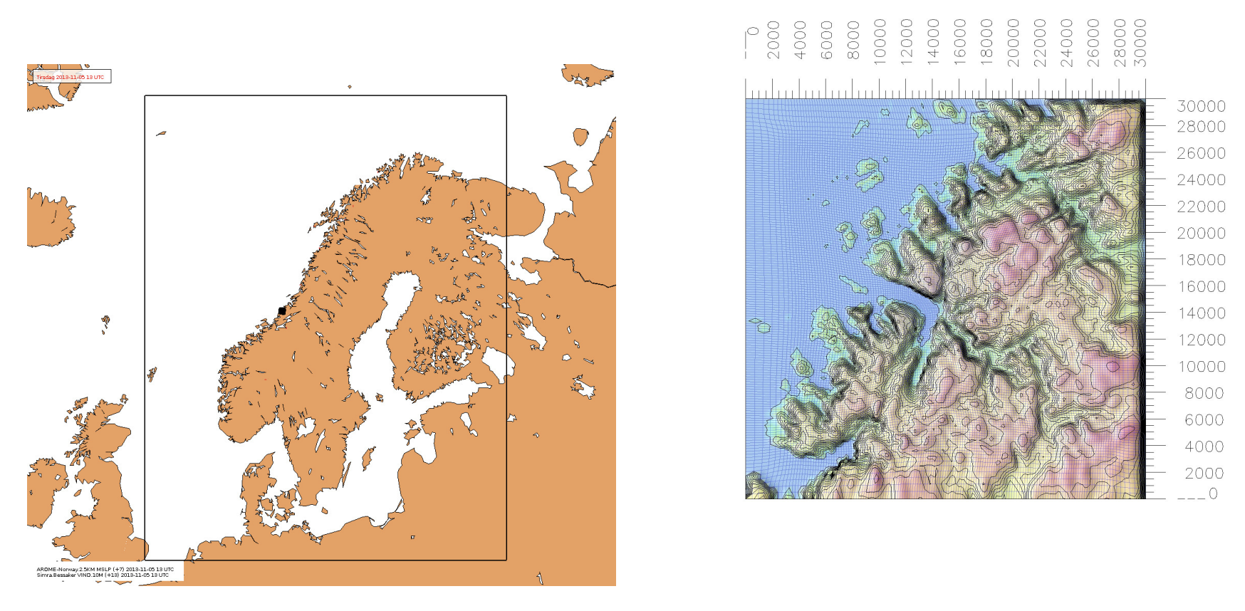
Figure 1: Area covered by the HARMONIE-SIMRA model, HARMONIE to the left, and SIMRA to the right, as it has been previously presented by Rasheed et. al. ⁴⁴

The hourly generated SIMRA data on a horizontal mesh with roughly $200m\times 200m$ resolution depending on the distance from the center of the mesh is available at https://thredds.met.no/thredds/catalog/opwind/catalog.html. This is the dataset that will be used as the original high-resolution wind field in this work.

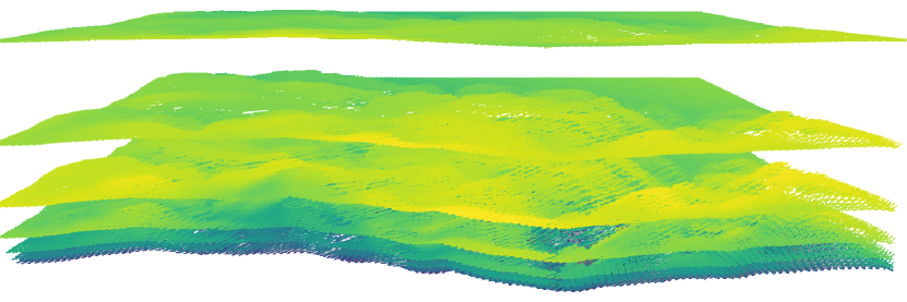
Figure 2: Shape of the dataset. Showing every fifth layer of data in the vertical coordinate. The $z$-coordinate has been multiplied by five to highlight the shape. Yellow marks high wind speed, and blue marks low wind speed.

Zooming in on a slice of the data set with $32\times 32\times 10$ points or 10 height layers with size $6.4\leavevmode\nobreak\ \mathrm{km}\times 6.4\leavevmode\nobreak\ \mathrm{km}$, and not scaling the vertical axis, the wind field is shown in more detail in Figure 3. It can be seen how the terrain affects the wind, causing higher wind speed uphill, and less, even reversed, wind speed downhill. Figure 3 also demonstrates how dense the horizontal layers are close to the ground, a normal property of simulated data, to help model the complexities of near-surface wind flow.

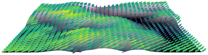
Figure 3: Zoomed in unscaled wind field. Showing the 10 bottommost layers in a 32x32 slice of the data area. Yellow marks high wind speed, and blue marks low wind speed.

For the purpose of this work, the unevenness in the vertical spacing is an advantage and a challenge at the same time. Higher information density in areas that are hard to approximate is beneficial for accurate modeling, and when designing wind farms one is interested in the wind speed relatively close to the ground, where turbines can harvest the wind energy. At the same time, it poses a challenge for applying CNNs, as they, in applying the same convolutional filter across the entire spatial dimension, assume that the same relations hold between neighboring points in one part of the data as others. If this is not the case, the CNNs have to compromise between features in different parts of space. To address this challenge, different approaches to handle the vertical spacing are tested and compared in Experiment 1, which is further explained in Section 3.6.

Zooming further, in Figure 4, some of the flow characteristics can be seen that make it hard to model near-surface wind fields in complex terrain. Dips and bumps in the landscape induce swirls and chaotic wind patterns. The figure adumbrates the difficulty of super-resolving the wind field, as a perfect generator would have to infer the full swirling pattern of the high-resolution wind field in Figure 4(a) from the low-resolution wind field in Figure 4(b). Comparing such areas in the generated and real data, therefore, provides a key indicator of how well the model has learned to model the physics of atmospheric wind flow.

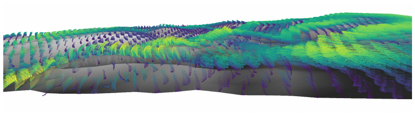
((a)) High-resolution wind field

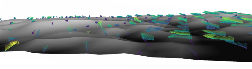
((b)) Low-resolution wind field

Figure 4: Turbulent Terrain effects. Showing the 16 bottommost layers in a chaotic region of the wind field.

These patterns also demonstrate an advantage of working with full 3D data rather than 2D slices, as these effects are hard to pick up from one 2D slice.

3.2 Data preprocessing

The SIMRA model is evaluated on a mesh with size $150\times 150\times 41$. The simulation tends towards low accuracy close to the edges due to relatively coarse resolution; therefore, the outermost points are discarded so that the horizontal dimensions are reduced to $128\times 128$ points. Furthermore, the wind field becomes more complex closer to the terrain. Due to limited computational resources available, this work focuses on 10 lower layers, where the wind flow prediction is most challenging (layers 2-11, the first layer is dropped as it represents the wind speed at height zero over the terrain which is always zero). Note that this restriction is motivated purely by available computational resources and does not limit the significance of the study since it can be assumed that flows in higher layers are easier to interpolate due to the relatively lesser influence of terrain on them. The resulting wind field can be formulated as an array with shape $128\times 128\times 10$.

While many distinct wind fields are available for training the generator and discriminator, the wind fields have all been calculated for the same terrain, which poses the risk of the NN to memorize the terrain. To reduce the potential for such overtraining, a smaller slice of the wind field is used for training, so that each wind field slice has a slightly different underlying terrain. The size of the slices is chosen to $64\times 64\times 10$ of the full $128\times 128\times 10$ terrain. This results in $65\times 65$ possibilities for taking a slice. If sampled uniformly, values at the edges are less likely to be included in the data set. To alleviate this, a beta distribution with $(0.25,0.25)$ is used for drawing samples. The probability of a pixel being included in the data set is shown in Figure 5. As the translation invariance of convolutional networks limits the effect of this strategy, the wind field is also horizontally mirrored and rotated in $90\degree$ steps, resulting in $65\times 65\times 2\times 4=33800$ potentially correlated but not identical terrains to draw wind fields from.

Next, the wind field is downsampled in horizontal directions to a lower resolution using the nearest-neighbor method. The downsampling factor in this work is 4 unless explicitly stated otherwise. The result is a high-resolution wind field (referred to as HR) with $64\times 64\times 10$ wind vectors as the generator target and a low-resolution wind field (referred to as LR) with $16\times 16\times 10$ wind vectors as the generator input.

Figure 5: Probability for pixels being included in a subsample using uniform and beta (0.25,0.25) distribution for subsample selection. The beta distribution shifts the probability towards the edges and is used here.

While overtraining of the terrain in the feature maps should be avoided, the generator should still have a chance to learn from the terrain corresponding to the input wind field. Therefore, the low-resolution input may also include as additional features the low-resolution height above the mean sea level, low-resolution terrain height, and/or height over the terrain in low resolution. Additionally, the low-resolution pressure can potentially contribute information and can be included as a feature in the low-resolution input. Each of these additional contributions can be toggled with a new hyperparameter, and the effect of each contribution is investigated as part of this work as explained in Experiment 1 in Section 3.6.

It is well known that normalizing data tends to ease the training of NNs, and so here too all values are normalized to $[0,1]$, except for vector components, which are normalized to $[-1,1]$. One additional hyperparameter is added that toggles whether all input values are interpolated in the vertical direction to be evenly spaced with respect to the ground. The preprocessed data is then used as input (LR) and target (HR) of the generator and as ground truth (HR) for the discriminator. Note that the 3D vector field is kept in a cartesian coordinate system so that the wind vectors are parametrized in $u_{x}$, $u_{y}$, and $u_{z}$. The data is split into training, validation, and test data set with ratios [0.8,0.1,0.1] respectively.

3.3 Model structure

The Generator and Discriminator architectures in this work are based on the ESRDGAN implementation ⁴⁵, which itself is based on the ESRGAN model by Wang⁴¹. The architectures of both networks are shown in Figure 6.

Generator

The generator uses the 3D low-resolution data (LR) and the high-resolution terrain height (Z) as input. The LR data is first processed by a 3D convolutional layer, whereafter multiple residual-in-residual dense blocks (RRDB) are stacked. An RRDB uses multiple residual dense blocks (RDB) which are implemented with residual connections, whose output is weighed with $\alpha=0.2$ before being added to the input. In the RDB, 3D convolutional layers with leaky rectified linear units (LReLU) activations are densely connected (after each output all previous inputs are summed up as input for the next layer). The RDB block finishes with a final convolutional network, whose output is weighted with $\alpha=0.2$ before being added to the input of the block. After the RRDB blocks, an additional convolutional layer is added, and a residual connection bypassing all RRDB is added. It follows upsampling convolutional blocks (UpConv) which are built from a nearest-neighbor upsampling (2x NN Up) and a convolutional layer with LReLU activation. Next, the output is concatenated with the terrain extractor, which takes the high-resolution terrain as input and extracts features through two convolutional layers where the first has LReLU activation. The concatenated output is processed by two final convolutional layers, where the former one has LReLU activation and a 3D feature dropout layer (Dropout3d). The output fo the final layer is then the super-resolved wind vector field (SR).

Discriminator

The discriminator uses downsampling convolutional blocks (DownConv), where each block starts with a convolutional layer with LReLU activation, followed by a depthwise separable convolutional layer for downsampling by a factor 2, batch normalization, and another LReLU activation. A modified DownConv block is added with separate stride widths for horizontal and vertical directions to account for unequal dimensions in the input data. The block is followed by a 3D dropout layer and two linear layers where the first uses LReLU activation.

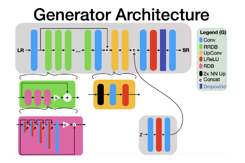
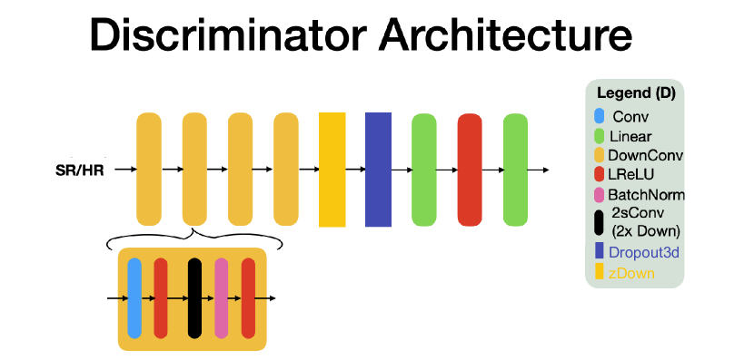
Figure 6: Generator and discriminator structure used in this work. A modified version of ERSDGAN ⁴⁵. Noteworthy changes are the increase from 2D to 3D, a new terrain feature extractor that takes high-resolution terrain information as input, additional feature dropout layers in the generator and discriminator, and the inclusion of a DownConv block with stride width 2 in vertical and 2 or 1 in horizontal direction depending on whether slice data augmentation is enabled or not.

3.4 Hyperparameters

Several hyperparameters have been changed from the original ESRGAN ⁴⁵, and from the earlier work on wind field interpolations ^{34, 35}. An exhaustive list of all default hyperparameters used in this work can be found in the appendix in Table LABEL:tab:full-fyperparameters. The hyperparameters are altered throughout the work only where mentioned explicitly. Specifically, in addition to the wind field, pressure and the $z$-coordinates of the data are included as low-resolution input channels to the generator. Data is augmented by slicing, mirroring, and rotating as specified in Section 3.2, and the generator and the discriminator are trained by alternating between them for 90k iterations. Instance noise is added to the input samples in the early training phase to confuse the discriminator, and one-sided label smoothing is included to prevent overconfidence inside the discriminator. A set of new hyperparameters that deserve special attention is connected to the choice of the loss function and is addressed in Section 3.5.

3.5 Loss

The Generative and Adversarial networks are trained by minimizing the respective loss function (also referred to as the cost function or objective function). In this work, the generator loss function $L_{G}$ is modified from the default setup and consists of several components, which are explained here. The first component is the pixel loss, which is calculated between each directional component of the vector in a certain position. Let $V^{HR}$ and $V^{SR}$ be the original high-resolution vector field and the reconstructed super-resolution vector field with horizontal components $V_{1},V_{2}$ and vertical component $V_{3}$. The pixel loss can then be written as a matrix

$$L_{G}^{pix}=\frac{1}{3}\sum_{i}^{3}\left|V_{i}^{HR}-V_{i}^{SR}\right|$$ (24)

with one value per vector in the (discrete) vector field.

In Section 2.1 it is shown that not only the vectors themselves but also the local partial derivatives are of importance. Therefore, a gradient-like loss matrix is calculated in the horizontal and vertical directions with

$$L_{G}^{grad_{x_{1}x_{2}}}={} \frac{1}{6}\min_{k\in\{1,2\}}\left(\frac{1}{N_{k}^{grad}}\right)\sum_{i}^{2}\sum_{j}^{3}\left(\frac{\partial}{\partial x_{i}}V_{j}^{HR}-\frac{\partial}{\partial x_{i}}V_{j}^{SR}\right)^{2}$$ (25)

$$L_{G}^{grad_{x_{3}}}={} \frac{1}{3N_{3}^{grad}}\sum_{i}^{3}\left(\frac{\partial}{\partial x_{3}}V_{i}^{HR}-\frac{\partial}{\partial x_{3}}V_{i}^{SR}\right)^{2}$$ (26)

where $\frac{\partial}{\partial x_{1}}$ and $\frac{\partial}{\partial x_{2}}$ are the derivatives in horizontal direction and $\frac{\partial}{\partial x_{3}}$ the derivative in vertical direction. $N^{grad_{x_{1}x_{2}}}$ and $N^{grad_{x_{3}}}$ are normalization factors that are calculated from the maximum value of all partial high-resolution and super-resolution derivatives $\frac{\partial}{\partial x}V$ involved in each equation through

$$N_{k}^{grad}={} \max\Biggl{(}\max_{j\in\{1,2,3\}}\left(\left|\frac{\partial}{\partial x_{k}}V_{j}^{HR}\right|\right),\frac{1}{100}\max_{j\in\{1,2,3\}}\left(\left|\frac{\partial}{\partial x_{k}}V_{j}^{SR}\right|\right)\Biggr{)}$$ (27)

Similarly to the gradient, the divergence in two and three dimensions is included in the loss through

$$L_{G}^{div}={} \min_{k\in\{1,2,3\}}\left(\frac{1}{N_{k}^{div}}\right)\left(\sum_{i}^{3}\frac{\partial}{\partial x_{i}}V_{i}^{HR}-\frac{\partial}{\partial x_{i}}V_{i}^{SR}\right)^{2}$$ (28)

$$L_{G}^{div_{x_{1}x_{2}}}={} \min_{i\in\{1,2\}}\left(\frac{1}{N_{i}^{div}}\right)\left(\sum_{i}^{2}\frac{\partial}{\partial x_{i}}V_{i}^{HR}-\frac{\partial}{\partial x_{i}}V_{i}^{SR}\right)^{2}$$ (29)

Again, the normalization factor is computed over all involved derivatives

$$N_{k}^{div}={} \max\Biggl{(}\max\left(\left|\frac{\partial}{\partial x_{k}}V_{k}^{HR}\right|\right),\frac{1}{100}\max\left(\left|\frac{\partial}{\partial x_{k}}V_{k}^{SR}\right|\right)\Biggr{)}$$ (30)

For each of the above loss matrices, the mean is then computed over all matrix components. In addition to the aforementioned components, the adversarial generator loss $L_{G}^{adv}$ is calculated based on the relativistic average discriminator as shown in Equation 14. The full loss $L_{G}$ of the generator can then be written as

$$L_{G}={} \eta_{1}L_{G}^{pix}+\eta_{2}L_{G}^{grad_{x_{1}x_{2}}}+\eta_{3}L_{G}^{grad_{x_{3}}}+\eta_{4}L_{G}^{div}+\eta_{5}L_{G}^{div_{x_{1}x_{2}}}+\eta_{6}L_{G}^{adv}$$ (31)

where $\eta_{1}$ to $\eta_{6}$ are the weights of each component with respect to the total loss and can be treated as additional hyperparameters. In contrast to the generator loss, the discriminator loss is calculated purely from the relativistic average adversarial loss in Equation 13.

3.6 Cases

As mentioned earlier, additional features and additional hyperparameters are introduced. The hyperparameter consists of weighting coefficients for the different components of the loss function. To tune these new hyperparameters and test the impact of features the following three experiments are conducted.

3.6.1 Experiment 1: Evaluating the impact of input features

First, the impact of various additional input features is tested. As touched upon earlier, the terrain shape and altitude significantly affect wind flow, but the irregular spacing of the vertical coordinates poses a problem for applying CNNs. This experiment aims to find the best way to address this, either by giving the generator input that contains information about the terrain, altitude, and vertical spacing or by interpolating the data vertically to get a more CNN-suited grid. To this end, the GANs are trained and evaluated with several combinations of pressure, absolute height, height over terrain, terrain height, and vertical interpolation as low-resolution input, while other parameters are kept as specified in Section 3.4. Two different seeds are used to estimate whether the results are reliable and can be reproduced.

Table 1: Combinations tested in Experiment 1. The column name is what the combination will be referred to, column interpolate indicates whether the data is interpolated vertically, while columns $z$, $p$, $z_{alt}$, and $z_{t}$ respectively refer to height above sea level, pressure, altitude, and terrain height respectively.

name	interpolate	$z$	$p$	$z_{alt}$	$z_{t}$
only_wind
$z$_channel		✓
$p$_channel			✓
$p\_z$_channels		✓	✓
$z_{ground}$_channels				✓	✓
$p\_z_{ground}$_channels			✓	✓	✓
only_wind_interp	✓
$z$_channel_interp	✓	✓
$p$_channel_interp	✓		✓
$z\_p$_channels_interp	✓	✓	✓

3.6.2 Experiment 2: Evaluating the impact of the loss components

Next, the second set of hyperparameters, the weights of the components that make up the loss functions, is investigated. In Experiment 2, the importance of the components is investigated by setting some weights to 0 while scaling up others, so that certain components of the loss function have higher contributions while others are deactivated. In addition to the loss function, another slightly modified configuration was made in response to the results of Experiment 1. The training ratio between the discriminator and generator (D_G_train_ratio) is changed to 2 after 60k iterations and niter to 100k so that the generator is trained for 60k+20k iterations and the discriminator is trained for 60k+40k iterations in total. Otherwise, the setup remains unchanged, i.e. only the pressure and height above mean sea level are added to the low-resolution input of the generator. In Experiment 2 the combinations of loss component weights $\eta_{i}$ in Table 2 are tested with two different seeds. The pixel loss and adversarial loss are kept constant at $\eta_{1}=0.15$ and $\eta_{6}=0.005$.

Table 2: Combinations tested in Experiment 2. The column name is what the combination will be referenced to as, and the other columns $\eta_{i}$s are the cost weighing constants defined in Equation (31)

name	$\bm{\eta_{2}}$	$\bm{\eta_{3}}$	$\bm{\eta_{4}}$	$\bm{\eta_{5}}$
only_pix_cost	0.0	0.0	0.0	0.0
grad_cost	1.0	0.2	0.0	0.0
div_cost	0.0	0.0	0.25	0.25
$xy$_cost	1.0	0.0	0.25	0.0
std_cost	1.0	0.2	0.25	0.25
large_grad_cost	5.0	1.0	0.25	0.25
large_div_cost	1.0	0.2	1.25	1.25
large_$xy$_cost	5.0	0.2	1.25	0.25

The std_cost combination is equivalent to the $p\_z$_channels combination in Experiment 1, so it will not be evaluated again, but this means that it hasn’t been changed as specified above, instead running 90k iterations for both discriminator and generator. The effect will be addressed in Section 4.

3.6.3 Experiment 3: Loss weight optimization

Following the fixed-value evaluation of the loss components, a hyperparameter search was conducted in the following search space which was chosen based on results of Experiment 2

$$0.0< \eta_{1}<1.0$$ (32)

$$0.5< \eta_{2}<32.0$$ (33)

$$0.25< \eta_{3}<16.0$$ (34)

$$0.25< \eta_{4}<16.0$$ (35)

$$0.25< \eta_{5}<16.0,$$ (36)

The search space is sampled logarithmically with base 2, except for $\eta_{1}$ which is sampled uniformly. The hyperparameter search is implemented using the ray tune framework ⁴⁶, with the Optuna ⁴⁷ optimizing framework and an Asynchronous Successive Halving Algorithm (ASHA) ⁴⁸ scheduler. The Optuna search algorithm implements a Bayesian tree search algorithm, it incorporates the results of previous samples when choosing configurations to test. The ASHA scheduler asynchronously stops poorly performing configurations, allowing tests of more combinations with the same computational resources. Note that this biases the search towards parameter combinations that result in good performance in the early training stages, and therefore assumes that strong initial performance indicates strong performance in later stages. Ray tune is a flexible framework for implementing the parallel processing of the search. The maximum training iterations is set to 35k and the minimum iterations before stopping a run is set to 1.2k. The search is initialized with promising combinations based on results from Experiment 2.

3.7 Software and hardware framework

All the data used in this project was available in a NetCDF (Network Common Data Form) file format through an OpenDap server hosted by the Norwegian Meteorological Institute. For processing the data NetCDF library was utilized. All the codes for the GANs framework were developed in Python 3.9.13 using the PyTorch 2.0.1 library, which is an open-source software library developed by Facebook’s AI group with a focus on the implementation of various neural network architectures.

The HARMONIE-SIMRA codes were run on the supercomputing facility “Vilje", which is an SGI Altix ICE X distributed memory system that consists of $1440$ nodes interconnected with a high-bandwidth low-latency switch network (FDR Infiniband). Each node has two 8-core Intel Sandy Bridge ($2.6\,\mbox{Ghz}$) and $32\,\mbox{GB}$ memory, yielding the total number of cores to $23040$. The system is applicable and intended for large-scale parallel MPI (Message Passing Interface) applications. The results are converted into NetCDF and realized through an OPeNDAP server. The use of OPeNDAP (Open-source Project for a Network Data Access Protocol) ⁴⁹ precludes the redundant copying of the results files on numerous machines for post-processing. A set of Python routines are implemented to read and post-process the hosted files on the fly. A brief overview of the computational set-up is given in Table A7. The HARMONIE model runs on $1840$ cores and to complete a $48$ hours forecast it takes approximately $87$ minutes. SIMRA on the other hand, running on $48$ cores, takes 13 minutes to finish one hourly averaged simulation each for the next $12$ hours.

The listed experiments and training of the models were done with NVIDIA A100m40 GPUs on the IDUN cluster at the Norwegian University of Science and Technology (NTNU). With one GPU, training the model for 100k iterations takes slightly less than two days. The GPU memory usage strongly depends on the input data size and the batch size. With batch size 32 and $16\times 16\times 10$ to $64\times 64\times 10$ interpolation, training the model requires approximately 22GB GPU memory. The full code and its history can be found on GitHub at https://github.com/jacobwulffwold/GAN_SR_wind_field. The results are reproducible using the repository. The code is modified from Larsen’s ³⁵ code, which again is an adaptation of Vesterkjær’s ⁴⁵ code that is accessible at https://github.com/eirikeve/esrdgan. All parts of the code have been modified, but Vesterkjær’s basic structure remains.

4 Results and discussions

In this section, the results of Experiments 1-3 are presented and discussed. The best combination of hyperparameters is identified, the model is evaluated with those hyperparameters, and the resulting wind fields are discussed in detail. Finally, the effects of overfitting the terrain and increasing the resolution enhancement factor are investigated.

4.1 Experiment 1: Evaluating the impact of input features

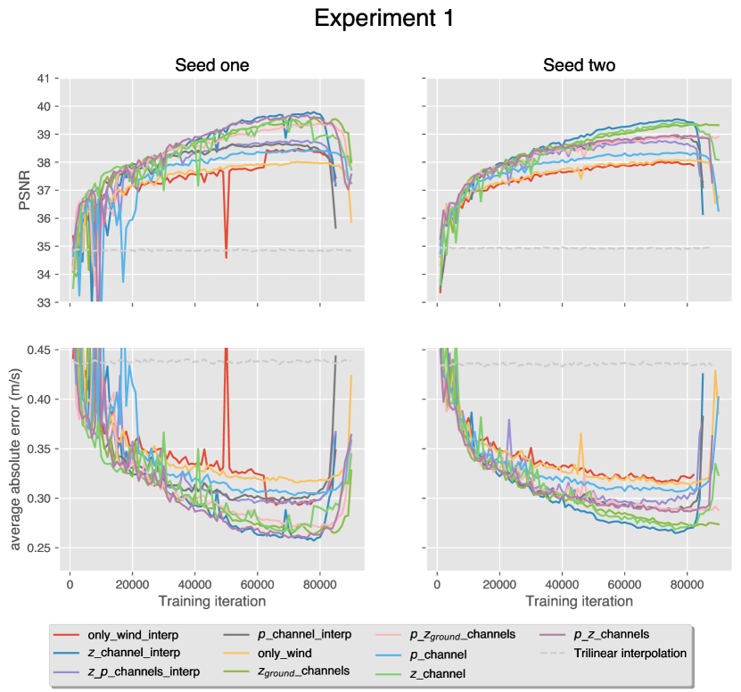
Figure 7: Experiment 1 validation results during training for two different seeds, colored according to the combinations specified in Table 1. The top row shows the validation peak signal-to-noise ratio, and the bottom row shows the average absolute error of a wind component of the generated wind field. A dashed line for trilinear interpolation performance is included for comparison.

The first experiment targets the additional input of the generator on two seeds as explained in Section 3.6. The peak-signal-to-noise ratio and average absolute error of each seed over the number of training iterations are shown in Figure 7. It can be immediately seen that all configurations perform significantly better than the trilinear interpolation and that the performances of all GANs follow a similar pattern during training. However, the performance significantly drops after around 80k training iterations (80k epochs), which was verified to be caused by the adversarial loss component. The reason for this phenomenon is that the contributions from all loss components except adversarial loss have become so small that adversarial loss dominates the error and explodes the network. This finding is the reason for the change in the training strategy in Experiment 2 and Experiment 3 as explained in Section 3.6.

The performance of the GANs saved at 80k training iterations is listed in Table A8. Note that in some cases, the degradation of performance already starts before reaching 80k epochs. For this reason, Figure 7 is used for the evaluation of the experiment. It can be seen that including pressure and/or any information on height improves the prediction over the only_wind setup. Interpolation of the input alone does not provide reproducible benefits. Adding only pressure results in minor benefits for both seeds. However, augmenting the input with altitude or height above mean sea level brings significant improvements. In both seeds, the five best-performing input constellations include some form of information on the height of the wind vectors either relative to terrain or to mean sea level. In both seeds, the best results are achieved by including the relative height above mean sea level and using interpolation, i.e. by setup $z$_channel_interp.

Limited computational resources prevented the evaluation of more seeds, which makes it impossible to draw more nuanced conclusions between input constellations. However, for this work, it is sufficient to identify the best performing model, to show that the generator based on convolutional layers performs well despite the irregular coordinates, and to prove that the quality of the generator can be improved by including information on the height of each wind vector in the input.

4.2 Experiment 2: Evaluating the impact of the loss components

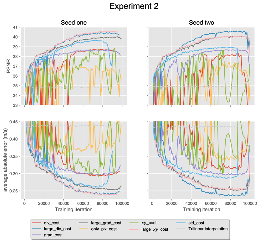
Figure 8: Experiment 2 validation results during training for two different seeds, colored according to the combinations specified in Table 2. The top row shows the validation peak signal-to-noise ratio, and the bottom row shows the average absolute error of a wind component of the generated wind field. A dashed line for trilinear interpolation performance is included for comparison.

The objective of Experiment 2 is to identify the most important components of the loss by adjusting the weights as explained in Section 3.6. Similar to Experiment 1, the peak-signal-to-noise ratio and the average absolute error are shown in Figure 8. The results of using the generator saved on the training iteration 80k for std_cost and 90k for the rest of the combinations in the test set are collected in Table A9. Again, Figure 8 is used for the main evaluation. As a response to the strong network degradation due to the adversarial loss at around 80k epochs in experiment 1, the discriminator was trained more frequently than the generator by only evaluating the generator every second training iteration. It can be seen in Figure 8 that still a degradation sets in at around 100k training iterations, which corresponds to training the generator for 80k epochs. The exception is the default configuration std_cost, which has not been retrained, and therefore experiences 80k generator epochs and, therefore, training collapse after 80k training iterations. Therefore, this approach did not prevent degradation. Furthermore, it can be seen that using only the pixel- and adversarial loss (i.e. only_pix_loss) results in very poor performance. Neglecting the derivatives in the vertical direction (i.e. combination $xy$_cost) results in bad quality of reconstructed wind fields too. Finally, training the GANs without gradient loss (div_cost) or divergence loss (grad_cost) reduces the quality of the predictions, albeit not as significantly. Large weights for any of the gradient components (large_grad_cost) divergence components (large_div_cost) and horizontal derivatives (large_$xy$_cost) represent the best constellations.

These observations suggest that most derivative-based loss components are important for optimal training. The exceptions are the vertical components of the gradient and divergence, where it has only been shown that one of them brings an important contribution, but no investigation has been carried out to separate them. While they could be inspected more closely here by introducing an additional constellation, their contributions are instead investigated as part of Experiment 3. Additionally, constellations with large weights on loss components perform better than the initial values. A learning rate that is smaller than optimal could cause this. Further investigation has shown that increasing the learning rate indeed improves performance.

4.3 Experiment 3: Loss weight optimization

In Experiment 3 the weights of each loss component are optimized by a hyperparameter search as explained in Section 3.6.3. The results of the parameter search can be seen in Figure 9. In the upper plot, all evaluated combinations are shown, while the lower plot gives a zoom-in on the region covered by the best-performing models according to PSNR. The loss weights of the five best-performing evaluations and their PSNR and pixel loss are shown in Table 3. Both Figure 9 and Table 3 show that high values for $\eta_{2}$, i.e. the gradient in the horizontal directions, are preferred over very high values for $\eta_{3}$ and $\eta_{5}$. The pixel loss weight $\eta_{1}$ and the divergence loss weight $\eta_{5}$ of the best-performing models span almost their whole parameter space, indicating rather low importance.

Table 3: Best performing combinations in Experiment 3. The $\bm{\eta_{i}}$s are the loss weighing constants defined in Equation 31, and PSNR and pix are the metrics as defined in Section 2.3.

$\bm{\eta_{1}}$	$\bm{\eta_{2}}$	$\bm{\eta_{3}}$	$\bm{\eta_{4}}$	$\bm{\eta_{5}}$	PSNR (db)	pix (m/s)
$0.336$	$30.6$	$1.86$	$7.21$	$3.66$	$39.9$	$0.259$
$0.757$	$22.6$	$3.05$	$11.2$	$4.45$	$39.6$	$0.265$
$0.446$	$26.4$	$0.643$	$1.18$	$0.62$	$39.5$	$0.271$
$0.231$	$20.9$	$0.565$	$0.398$	$1.76$	$39.5$	$0.277$
$0.477$	$21.4$	$0.464$	$0.965$	$0.391$	$39.4$	$0.271$

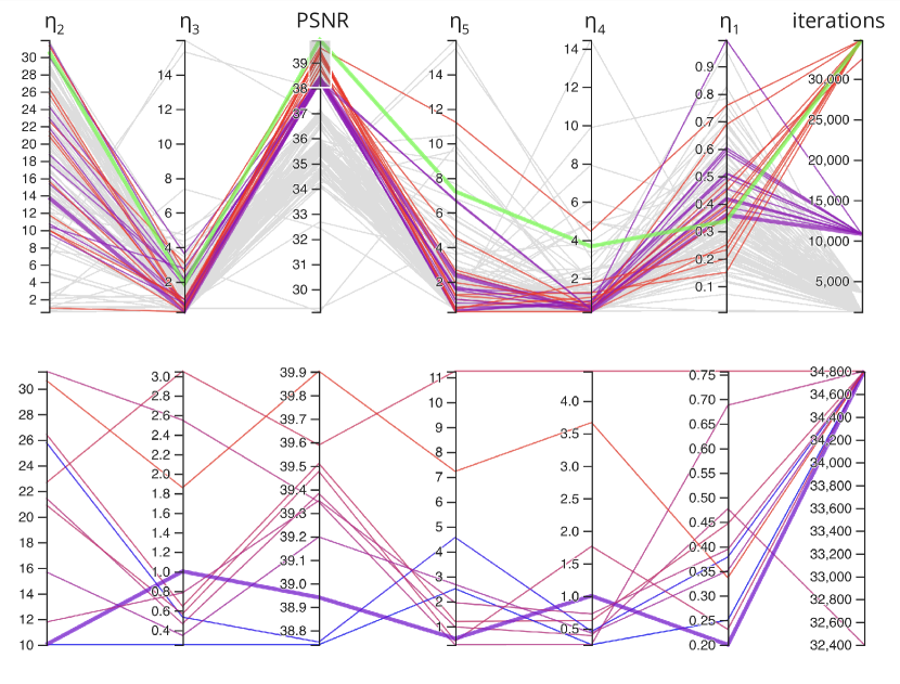
Figure 9: Results of Experiment 3. In the upper plot, the scores of all tested combinations and their parameters are displayed, with the best-performing combinations highlighted. The $\eta_{i}$s are the loss weighing constants defined in (31), "iterations" is what iteration the run was stopped at, and PSNR is the validation PSNR score after that iteration. In the bottom plot, we see the same table for only the best performers with the parameter axes scaled according to their spanned parameter range. Plot generated with ray.tune.

Note that the weights just determine the scaling of the loss component. To identify which losses actually contribute most to the optimization, the weighted loss components are evaluated separately during training on the validation data set and shown for the best-performing model in Figure 10. The loss is dominated by the horizontal gradient component $L^{grad_{xy}}$ and the horizontal divergence $L^{div_{xy}}$ but also experiences contributions from the full divergence $L^{div}$. The pixel loss component $L^{pix}$ and vertical gradient component $L^{grad_{z}}$ have minor contributions in the early training stage, but quickly decay. The adversarial loss has barely any contributions throughout the 35k iterations and does not change except for minor fluctuations in the first 3k and last 500 epochs. Subsequent testing showed that the steep drop in performance around 80k epochs of generator training is, in fact, caused by the discriminator loss. At 80k epochs, all other loss components are optimized to the point where the adversarial loss becomes the main component of the loss. Further investigation showed that this drop can be prevented by adjusting the hyperparameters of the discriminator, which will be discussed in more detail in Section 4.4.

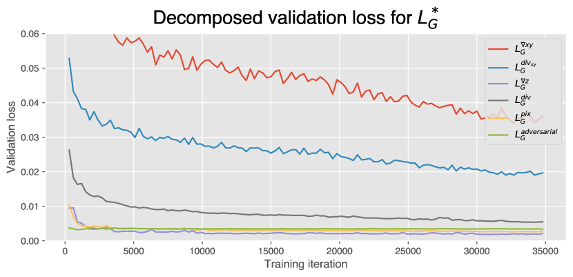
Figure 10: Decomposed validation loss for the best-performing loss weights in the parameter search. The loss components in the plot are as the ones defined in Equation 31.

4.4 Evaluation of the best model

4.4.1 Hyperparameter adjustment

Based on the results of Experiment 1, Experiment 2, Experiment 3 and further testing, a number of changes were made to the hyperparameters of the model. Experiment 1 gives reason to remove the pressure from the generator input, while Experiment 2 and Experiment 3 motivate to adjust the learning rate and the loss-component weights. Most significantly, adversarial learning has been dropped. While the degradation in training around 80k epochs reported earlier can be prevented by adjusting the alternation between generator and discriminator training from every epoch to every 50th epoch, changing the interval between the training of discriminator and generator, experimenting with turning on or off instance noise and label smoothing, adjusting the adversarial loss weight, and initiating with a generator pre-trained on content loss gave no significant increase in performance compared to the loss function with purely physically-motivated loss components. Therefore, the best model architecture in this work is the one without adversarial learning. Note that this means that the best super-resolution neural network in this work is a generative convolutional network, but not a generative adversarial neural network. In fact, it is a major result of this work that the physics-based loss components perform so well that including adversarial losses does not further improve performance.

The other loss component weights are set according to the best-performing values from Experiment 3, but normalized by a factor of 10, except for the $L^{grad_{z}}$ component, which had negligible contributions to the total loss, and the pixel loss weight $\eta_{1}$, which was set dynamically. The generator was first trained for 100k iterations with pixel loss $\eta_{1}=0.034$ and then trained for 150k iterations with $\eta_{1}=0.136$. Restarting with four times as high pixel loss not only improved pixel-wise error but also caused lower gradient-based losses. Furthermore, while improving the PSNR and pixel error, larger loss weights with constant learning rate result in larger gradients in the loss, i.e. larger steps per evaluation. However, this collides with the gradient clipping previously employed. In fact, clipping results in constant gradients for almost all evaluations throughout the full training, which causes a significantly slower parameter change than the gradients suggest. Therefore, the learning rate here was increased by a factor of 8, and gradient clipping was dropped. The full set of modified generator parameters is listed in the appendix in Table A10. Otherwise, the generator setup is unchanged from the full list of hyperparameters in the appendix in Table LABEL:tab:full-fyperparameters.

4.4.2 Metrics and Overall Performance

The average test scores of the final model are compared against the trilinear interpolation in Table 4. With the adjusted parameters, the generator achieves even higher PSNR and lower pixel error. Additionally, the absolute error of the vector length in 3D, i.e. the "pixel vector" of the vector length, pix-vector, and the pix-vector relative to the maximum wind speed in the sample are shown. The generator achieves significantly better results than the trilinear interpolation on all metrics.

Table 4: Test result of the final model. Metrics are defined in Section 2.3. Though being interpolated, the generated wind field is not interpolated back and compared to the original data as in Table A8, as this did not affect the results significantly. Trilinear interpolation performance is included for comparison.

Interpolation	Trilinear	Generator
PSNR (db)	36.35	47.14
pix (m/s)	0.385	0.116
pix-vector (m/s)	0.80	0.24
pix-vector relative	18.5%	6.12%

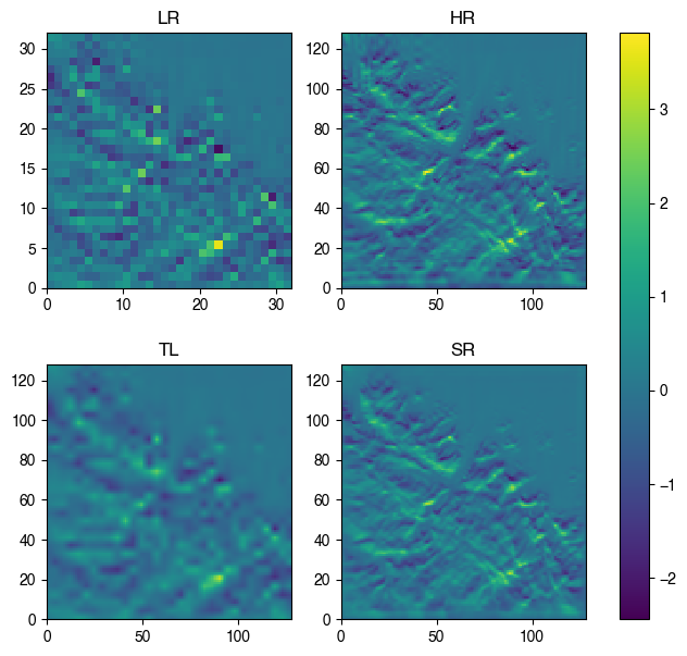
((b)) Wind velocity along the $z$-axis

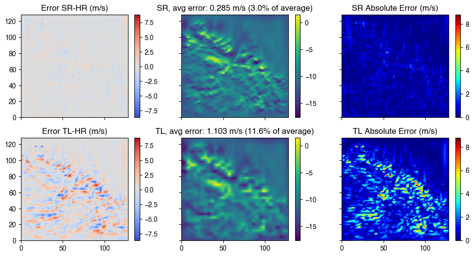
((c)) Error for wind velocity along the $x$-axis

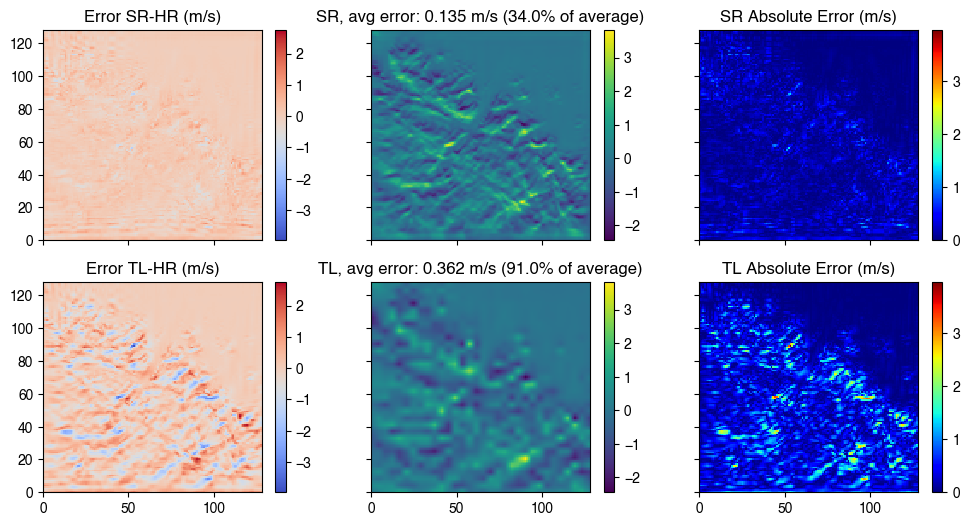
((d)) Error for wind velocity along the $z$-axis

Figure A17: Comparison of the second highest horizontal 2D slice of the wind field for a randomly selected wind field. LR means low resolution, the input of the model, TL means trilinear interpolation of the LR data, SR means the super-resolved wind field generated by the trained network and HR means the true high resolution wind field. "Avg error" refers to average absolute error for the displayed wind component in the displayed slice, the "% of average" means this value divided by the average of value of that wind component in that slice for the HR wind field.

In Figure 11 the second lowest horizontal layer of the 3D wind field can be seen in low resolution (LR), high resolution (HR), trilinear interpolated (TL), and super-resolved by the generator (SR). The generator adds finer details to the reconstructed image that the trilinear interpolation cannot capture and includes information from the underlying terrain. More importantly, the relative and absolute error of the wind in both horizontal and vertical directions is reconstructed significantly better by the generator. The same figure for the second-highest horizontal layer of the wind field can be found in the appendix as Figure A17.

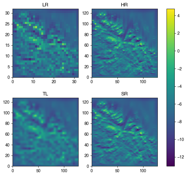
((a)) Wind velocity along the $x$-axis

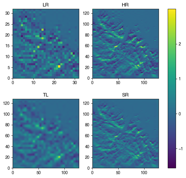
((b)) Wind velocity along the $z$-axis

((c)) Error for the wind component pointing along the $x$-axis

((d)) Error for the wind component pointing along the $z$-axis

Figure 11: Comparison of the second lowest horizontal 2D slice of the wind field for a randomly selected wind field. LR means low resolution, the input of the model, TL means trilinear interpolation of the LR data, SR means the super-resolved wind field generated by the trained network and HR means the true high-resolution wind field. “Avg error" refers to the average absolute error for the displayed wind component in the displayed slice, the "% of average" means this value divided by the average value of that wind component in that slice for the HR wind field.

4.4.3 Generated 3D Wind Field

Next, the entire wind field is compared in 3D. In Figure 12 a sample with a mean wind speed at 8.2 m/s is investigated. For this wind field, the average length of the error wind vector of the SR field is 0.41 m/s (5% of average) and the average absolute error of the TL field is 1.34 m/s (16% of average). In figure Figure 12 it can be seen how the generated wind fields adapt to the terrain, comparing LR, HR, TL, and SR data, as before.

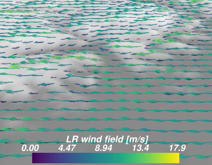
((a)) LR wind field

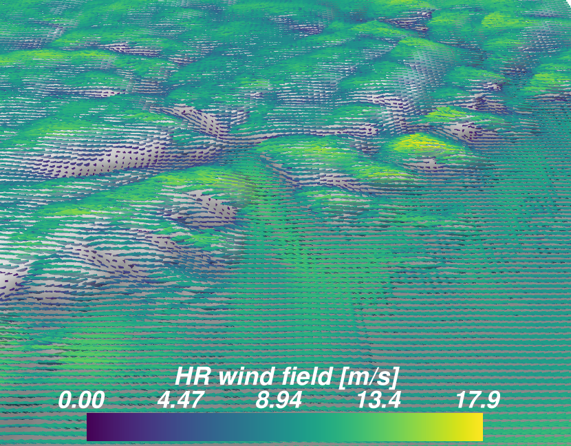
((b)) HR wind field

((c)) TL error, HR-TL

((d)) SR error, HR-SR

((e)) TL wind field

((f)) SR wind field

Figure 12: Comparison of LR, HR, TL, and SR wind fields from a randomly selected sample with high average wind speed. LR means low resolution, the input of the model, TL means trilinear interpolation of the LR data, SR means the super-resolved wind field generated by the trained network and HR means the true high-resolution wind field.

Figure 12 demonstrates that the super-resolved wind field adapts much more crisply to the terrain than the interpolated data. The trilinear interpolation error plot in Figure 12(c) follows regular terrain patterns, with the interpolation systematically misjudging regions of rapidly changing terrain. Meanwhile, Figure 12(d) captures even fast-changing terrain patterns well, and the smaller error is more randomly distributed, indicating that the generator performs well regardless of terrain features. The model, however, is trained to minimize absolute error in gradients and component-wise wind speed, which means that for any batch during training, the larger wind fields dominate the loss function. Therefore, Figure 13 shows a sample with an average wind speed of 1.04 m/s.

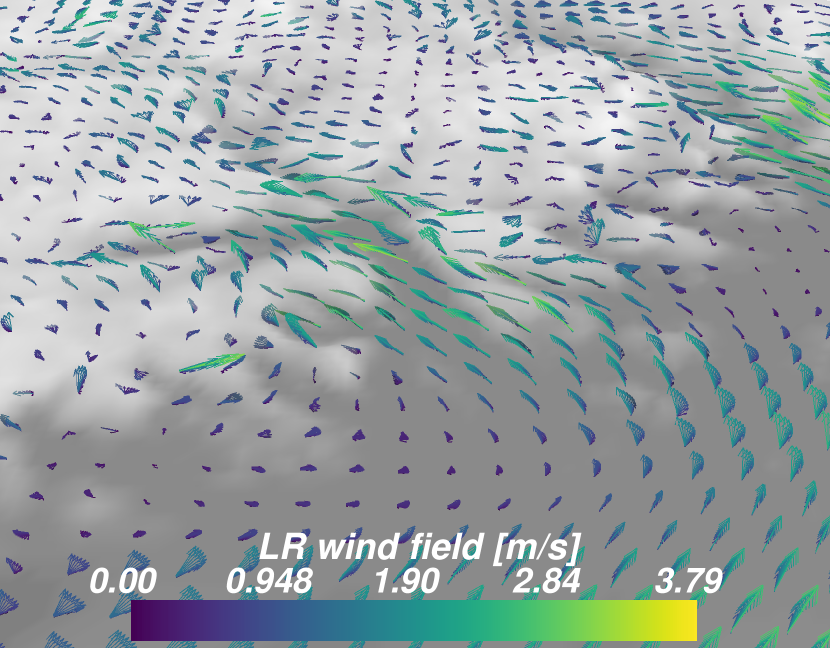
((a)) LR wind field

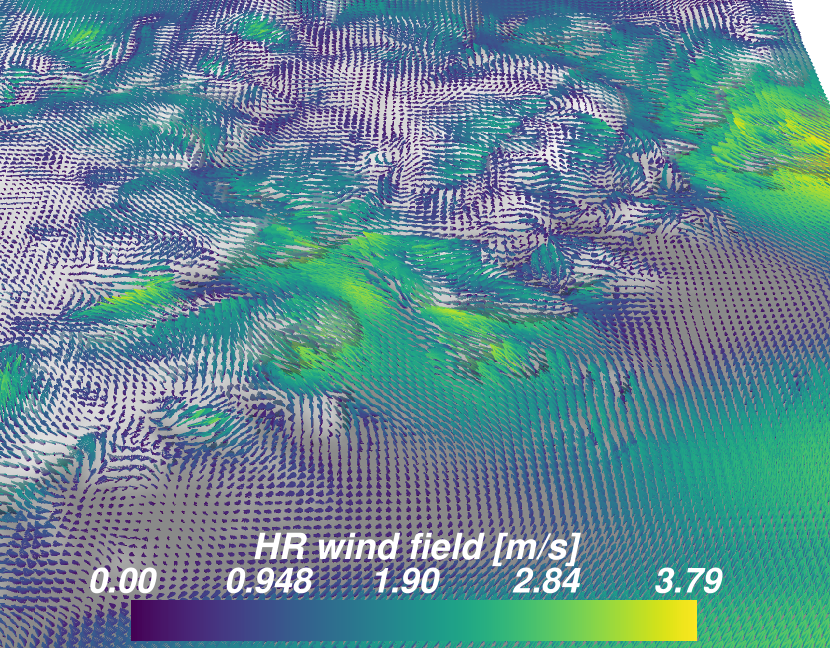
((b)) HR wind field

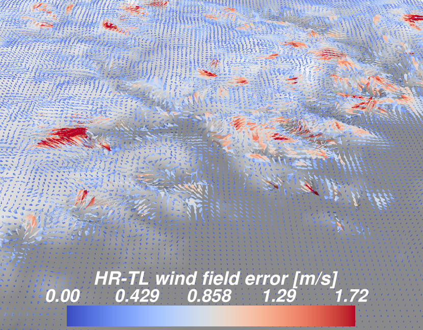
((c)) TL error, HR-TL

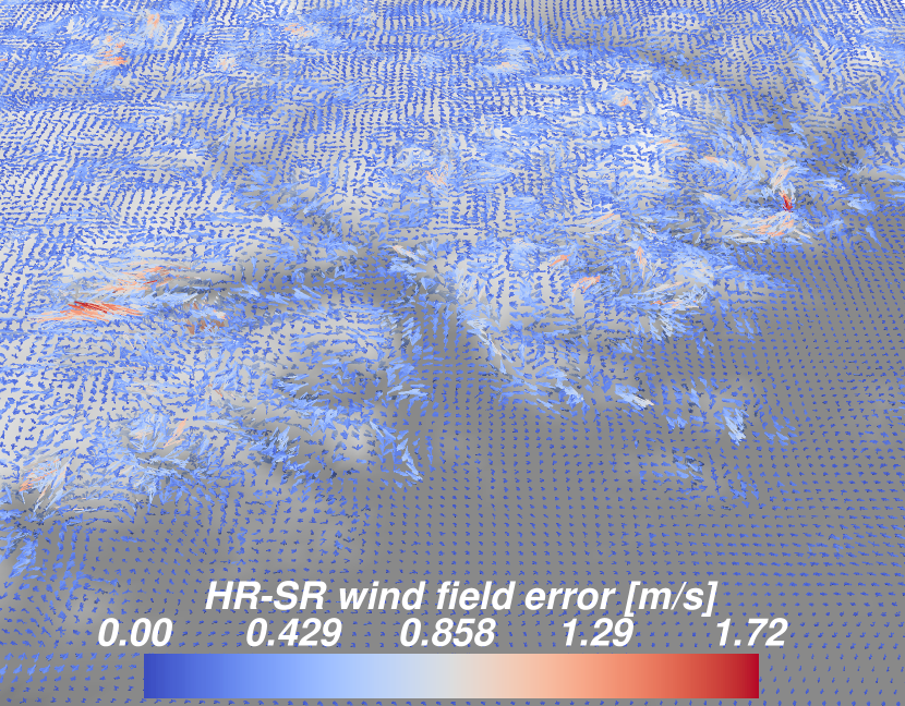
((d)) SR error, HR-SR

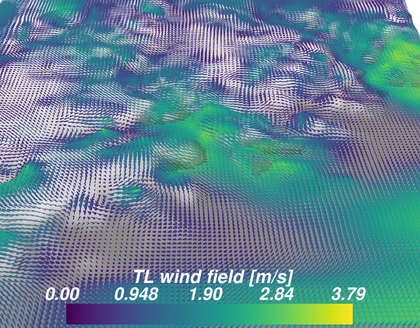
((e)) TL wind field

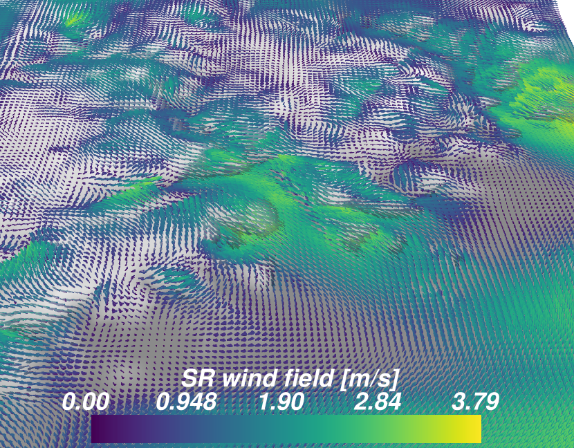
((f)) SR wind field

Figure 13: Comparison of LR, HR, TL, and SR wind fields from a randomly selected sample with low average wind speed. LR means low resolution, the input of the model, TL means trilinear interpolation of the LR data, SR means the super-resolved wind field generated by the trained network and HR means the true high-resolution wind field.

For this area, the average absolute error is 0.19 m/s (18% of average speed) for the generated super-resolution win field and 0.31 m/s (30% of average speed) for the interpolated wind field, i.e. a lower absolute error but a higher relative error for trilinear interpolation and generated super-resolution wind field. Comparing Figure 13(d) and Figure 13(e) more closely, it can be seen that the super-resolution field is performing worse than trilinear interpolation in quite large areas of low wind speed but still, the maximum and average error is smaller than that of triangular interpolation. It can be concluded that the model’s emphasis on absolute error makes it perform worse on very weak wind fields. However, this is desirable as the absolute error is generally more important in the context of wind fields.

Figure 13 also demonstrates a problem with the vertical cutoff of the training data. In the figure, there are large areas in which the wind seems to stop completely. Here the wind is pushed upwards by the terrain. With terrain-following coordinates only up to 40m above ground level and weak winds, the data doesn’t cover the wind continuing higher up, instead making it seem like the wind only blows at the top of hills. Given that this work tries to push the model towards learning traits like mass conservation, this is not ideal. Extending the input data to higher altitudes above ground may therefore improve the performance.

Turbulent effects in the wind field are investigated in Figure 14, which zooms in on a turbulent region of the high-resolution (HR), low-resolution (LR), trilinear interpolated (TL), and super-resolved (SR) wind fields.

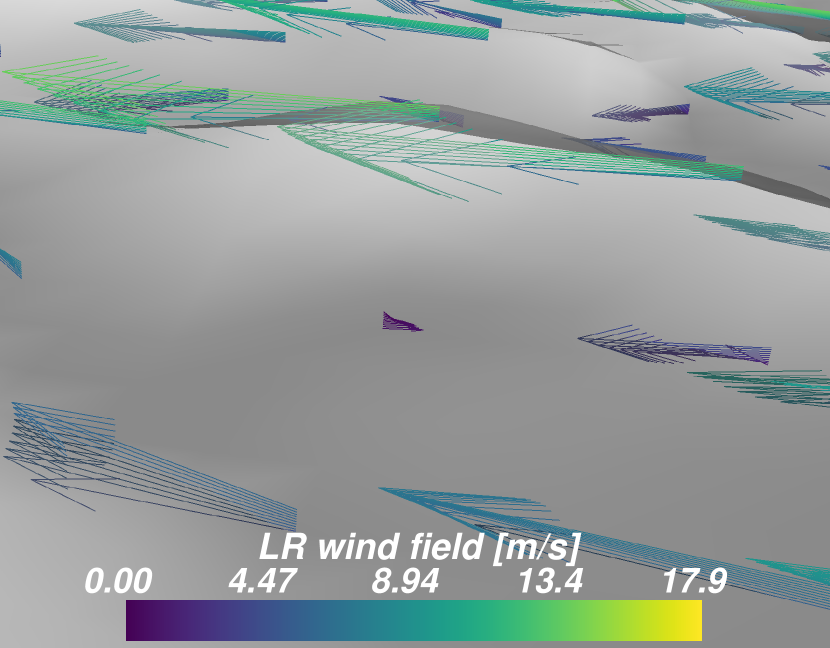
((a)) LR wind field

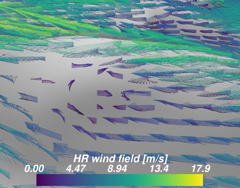
((b)) HR wind field

((c)) TL error, HR-TL

((d)) SR error, HR-SR

((e)) TL wind field

((f)) SR wind field

Figure 14: Comparison of LR, HR, TL and SR wind fields in a turbulent region. LR means low resolution, the input of the model, TL means trilinear interpolation of the LR data, SR means the super-resolved wind field generated by the trained network and HR means the true high resolution wind field.

While interpolation almost completely smoothes out the turbulence area, the super-resolved wind field is remarkably accurate. With only the datapoints in Figure 14(a) it recreates the swirling pattern of Figure 14(b), albeit slightly more regular than the actual data.

4.5 Influence on super-resolution achieved

Two more tests are carried out with the final configuration. First, higher upsampling factors are targeted, and second, the data slicing, i.e. predicting only a subset of the wind full wind field per evaluation, is turned off. Table 5 shows the results of super-resolving with a 4x4, 8x8, and 16x16 resolution increase with and without data slicing. It can be clearly seen that the model performs better when data-slicing is disabled, which likely results in one single terrain being overfitted. While this is not desirable when learning underlying equations, it can be used in digital twins to be trained with a pre-computed data set, and upsample low-resolution data to wind flow with high accuracy in real-time, which is impossible with numerical codes.

Furthermore, the results show that big resolution increases can be achieved while still producing reliable super-resolved wind fields. Especially when overtraining a single terrain, the generator achieves better performance on a 16x16 resolution increase than the trilinear interpolation for a 4x4 resolution increase. However, while this shows the benefits of overfitting the generator, it also raises the question of to what degree the data-slicing is able to reduce said overfitting. While several data augmentation measures have been taken to avoid this, the training set is still biased towards one terrain, and evaluation on an unseen terrain would be needed to investigate the potential overtraining further.

Table 5: Test results depending on varying resolution increase and whether data slicing is used in training. Though being interpolated, the generated wind field is not interpolated back and compared to the original data as in Table A8, as this did not affect the results significantly. Trilinear interpolation performance is included for comparison.

name	PSNR (db)	pix (m/s)	pix-vector (m/s)	pix-vector relative
$4\times 4$ SR	47.14	0.116	0.24	6.1%
$4\times 4$ SR no slicing	49.27	0.090	0.19	5.0%
$4\times 4$ TL	36.35	0.385	0.8	18.5%
$8\times 8$ SR	41.95	0.204	0.43	11.3%
$8\times 8$ SR no slicing	44.25	0.159	0.33	9.1%
$8\times 8$ TL	33.86	0.528	1.12	25.8%
$16\times 16$ SR	34.2	0.502	1.11	26.68%
$16\times 16$ SR no slicing	41.57	0.216	0.46	12.8%
$16\times 16$ TL	32.77	0.609	1.29	30.6%

In Figure 15 we compare the results of $8\times 8$ and $16\times 16$ resolution increase when not slicing the wind field, for the same horizontal layer as in Figure A17. Even with $8\times 8$, many details in the wind field can be recovered through the high-resolution terrain.

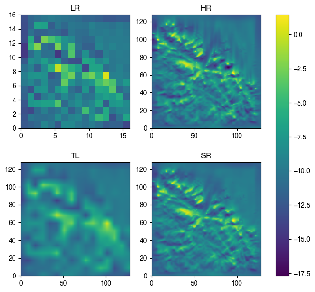
((a)) Wind velocity for 8x8 resolution increase

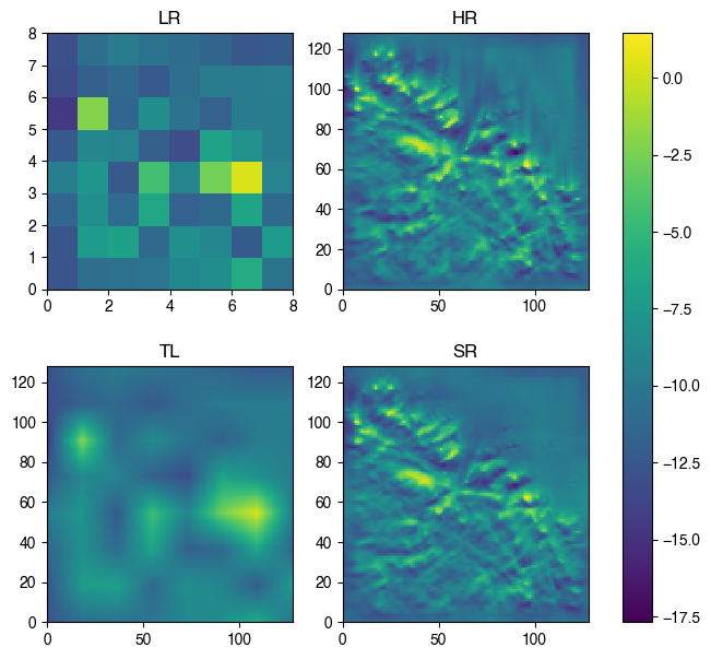
((b)) Wind velocity for 16x16 resolution increase

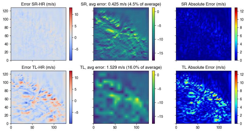
((c)) Error for 8x8 resolution increase

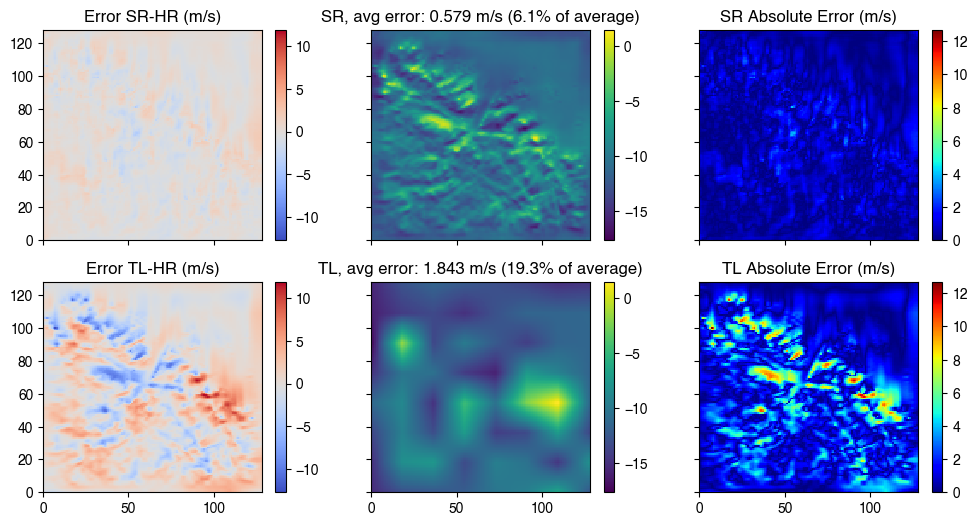
((d)) Error for 16x16 resolution increase

Figure 15: Comparison of 8x8 and 16x16 resolution increase for models trained without slicing on wind velocity along the $x$-axis for the second highest horizontal 2D slice of the wind field for the same wind field as in Figure A17. LR means low resolution, the input of the model, TL means trilinear interpolation of the LR data, SR means the super-resolved wind field generated by the trained network and HR means the true high-resolution wind field. "Avg error" refers to the average absolute error for the displayed wind component in the displayed slice, the "% of average" means this value divided by the average value of that wind component in that slice for the HR wind field.

5 Conclusion and future work

This paper presented a neural-network-based 3D wind flow super-resolution algorithm which was successfully applied to reconstruct a simulated 3D wind field of a Norwegian coastal area with a complex topography. The super-resolving neural network was based on the ESRGAN ⁴¹, however, several modifications were made to the architecture and hyperparameters. The GAN architecture was improved to process unevenly spaced 3D vector fields as input, and a terrain feature extractor was incorporated to supply the GAN with high-resolution terrain information. Additionally, a feature dropout layer was added to the generator, and the value of complementary input information in the form of height and pressure was explored. Moreover, major changes were made to the loss function. The main findings can be enumerated as follows:

1. Microscale 3D atmospheric wind flow can be well approximated by CNNs from low-resolution wind data and high-resolution terrain data even if the data is irregularly spaced vertically. The final generator was evaluated on a test set of wind fields with a peak signal-to-noise ratio of 47.14 db, an average length error in wind vector length of 0.24 m/s, and a relative wind speed error of 6.12%. The generator outperformed trilinear interpolation by far, which scored 36.42 db, 0.80 m/s, and 18.5% respectively. The model kept consistently outperforming trilinear interpolation even when the resolution enhancement was increased to $8\times 8$ and $16\times 16$, especially if the generator is applied on the same terrain that it was trained on.

2. Loss functions comparing specific parts of the wind gradient of the generated and high-resolution wind fields significantly improved performance, with gains from adversarial learning being negligible in comparison. The perceptual loss component of the ESRGAN has been replaced by physically motivated gradient- and divergence-based loss components. It was proven that the physically motivated loss greatly increases the performance of the super-resolution generator, to the point where training the generator without adversarial loss did not reduce the performance. This motivated using a generative model over a generative adversarial model for the final model configuration.

3. The proposed fully convolutional 3D generator with wind gradient-based loss function superresolves the near-surface 3D wind field strikingly well, both in terms of quantitative error and visual appearance.

Although these results are encouraging, there is room for further improvement in the following ways:

1. The high-resolution terrain feature extractor was implemented, but its architecture was not fully optimized. The ESRGAN in this work could be compared to an encoder-decoder structure such as that employed in the U-net ⁵⁰. The U-net starts and finishes with the same spatial dimensions, which would allow to include the high-resolution terrain in the same layer as a trilinear interpolated low-resolution wind field. On one hand, this allows the high-resolution terrain to be injected close to the low-resolution wind field, but on the other hand, information might degrade faster, and the interpolated wind field reduces the information density, especially for large zoom factors.

2. The results of this work discourage the use of adversarial approaches, as opposed to informed content loss. Working with adversarial training is more computationally demanding and potentially less stable (e.g. due to mode collapse and reproducibility). Nonetheless, carefully fine-tuned adversarial learning could bring benefits in the late stages of the training when physically motivated losses yield no further improvement. Additionally, a loss based on discriminator feature maps could be beneficial if the discriminator performs reasonably well. Using the feature extractor of a pre-trained discriminator or of the discriminator saved at some interval during training to add a feature loss might, for instance, give better granularity to the adversarial feedback.

3. Finally, the model is trained to interpolate from low-resolution fields that were artificially generated by downsampling a high-resolution simulation. However, the downsampled wind field likely has higher accuracy than any low-resolution simulation could achieve. Therefore, it needs to be tested whether the model can still infer high-resolution information even when the input is a true low-resolution simulation. Such a low-resolution simulation will likely have fewer vertical layers, which will require vertical interpolation as well.

Once the network has been validated for interpolation using the output of real low-resolution models as input, its fast evaluation allows it to be applied in real-time inside digital twins. The implementation of the high-resolution wind field into a digital twin accessed through a virtual reality interface is demonstrated in 16. Inside the digital twin, the prediction can be used directly for power forecasting, as has been demonstrated in ⁶, or can be used as input to models for wakes and structural responses.

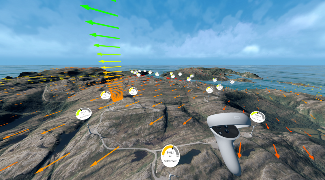
Figure 16: A high-resolution wind field implemented into a digital twin of the Bessakerfjellet wind farm. Here the digital twin is being accessed through a virtual reality headset.

Despite the potential for further research, the proposed model should be considered as a proof-of-concept for CNN-driven superresolution of 3D microscale atmospheric wind flow.

Appendix A Additional Tables and Figures

((a)) Wind velocity along the $x$-axis

Table A6: Full list of standard hyperparameters with explanation

General Parameters
Parameter	Value	Meaning/Comments
include_pressure	True	G input channel
include_z_channel	True	G input channel
included_z_layers	1-10	10 of the 11 layers closest to the ground (dropping the one furthest down)
conv_mode	3D	Alternatives: 3D, 2D, Horizontal3D (separate kernel for each horizontal layer)
interpolate_z	False	Interpolate as specified in Section 3.2
include_altitude_channel	False	include $z_{alt}$ as G input channel
load_G_from_save	False	Initialise G with a model trained without adversarial cost
Data-related parameters
Parameter	Value	Meaning/Comments
enable_slicing	True	Slice 64x64 slices as specified in Section 3.2
scale	4	$xy$ dimension scale difference between LR and SR, e.g. 16x16 $\rightarrow$ 64x64
batch_size	32
data_augmentation_flipping	True
data_augmentation_rotation	True
Architecture
Parameter	Value	Meaning/Comments
G/both D	G/both D
num_features	128 32	D features double for every DownConv block except the last
terrain_number_of_features	16	Number of features in the terrain feature extractor part of G
num_RRDB	16
num_RDB_convs	5	RDBs per RRDB
RDB_res_scaling	0.2	Residual scaling, $\alpha$ in the pink part of Figure 6
RRDB_res_scaling	0.2	Residual scaling, $\alpha$ in the green part of Figure 6
hr_kern_size	5	Kernel size after upscaling in the generator (5x5x5)
kern_size	3	Standard kernel size (3x3x3)
weight_init_scale	0.1 0.2	Smaller kaiming weight initialization
lff_kern_size	1	local feature fusion layer of RDB
dropout_probability	0.1 0.2
G_max_norm	1.0	Maximum gradient due to gradient clipping
Training
Parameter	Value	Meaning/Comments
G/both D	G/both D
learning_rate	1e-5 1e-5
adam_weight_decay_G	0 0
adam_beta1_G	0.9 0.9
adam_beta2_G	0.999 0.999
multistep_lr	True	Reduce learning rate during training
multistep_lr_steps	[10k, 30k, 50k, 70k, 100k]	schedule for reducing learning rate during training
lr_gamma	0.5	factor of reduction when lr is adjusted
gan_type	relativisticavg	Section 2.2
adversarial_loss_weight	0.005	$\eta_{6}$, as specified in Equation (31)
gradient_xy_loss_weight	1.0	$\eta_{2}$, as specified in Equation (31)
gradient_z_loss_weight	0.2	$\eta_{3}$, as specified in Equation (31)
xy_divergence_loss_weight	0.25	$\eta_{5}$, as specified in Equation (31)
divergence_loss_weight	0.25	$\eta_{4}$, as specified in Equation (31)
pixel_loss_weight	0.15	$\eta_{1}$, as specified in Equation (31)
d_g_train_ratio	1	How often D is trained relative to G
use_noisy_labels	False	Add noise to labels when training D
use_label_smoothing	True	Set HR labels to $0.9+0.1\frac{it}{it_{max}}$ instead of 1.0 when training D
flip_labels	False	Randomly flip (set HR_label=false, SR_label=True) some labels when training D
use_instance_noise	True	Add instance noise when training D, $\mathbf{D}(\mathbf{x})\rightarrow\mathbf{D}(\mathbf{x}+\bm{\epsilon})$
		$\bm{\epsilon}_{i}\sim\mathcal{N}\left(0,\,2.0\left(1-\frac{it}{niter}\right)\right)$
niter	90k	Number of training iterations
train_eval_test_ratio	0.8	Ratio for training, remaining fraction split equally between validation and testing

Table A7: Details of the computational models, number of CPU, domain extent [km], number of mesh elements [million], and total simulation time [minutes].

Model	CORES	Domain	N	Time
HARMONIE	1840	$1875\times 2400\times 26$	46	87
SIMRA	48	$30\times 30\times 3.0$	1.6	13

Table A8: Test results of Experiment 1. name references the combinations in Table 1. 1 and 2 refer to the two different seeds used for training. Since the models working with interpolated low-resolution data are trained to produce interpolated high-resolution data, the generated data is interpolated back to the original coordinates and evaluated against the original high-resolution data during testing. Those results are to the right, and evaluation results against the interpolated high-resolution data are to the left in the "interp" rows. Trilinear interpolation performance is included for comparison.

name	PSNR1 (db)	PSNR2 (db)	pix1 (m/s)	pix2 (m/s)
only_wind	39.35	39.32	0.283	0.285
$z$_channel	39.96	40.52	0.268	0.246
$p$_channel	39.59	39.65	0.278	0.276
$p\_z$_channels	40.27	40.05	0.253	0.261
$z_{ground}$_channels	40.6	40.61	0.242	0.244
$p\_z_{ground}$_channels	40.54	40.00	0.245	0.264
only_wind_interp	39.06 / 39.10	39.25 / 39.22	0.293 / 0.292	0.288 / 0.289
$z$_channel_interp	40.59 / 40.53	40.65 / 40.61	0.246 / 0.247	0.243 / 0.243
$p$_channel_interp	39.47 / 39.49	40.03 / 39.99	0.283 / 0.289	0.265 / 0.267
$z\_p$_channels_interp	39.73 / 39.75	39.77 / 39.77	0.274 / 0.274	0.276 / 0.273
trilinear	36.53		0.377
trilinear_interp	36.35 / 36.42		0.385 / 0.382

Table A9: Test results of Experiment 2. name references the combinations in Table 2, PSNR and pix are metrics defined in Section 2.3, and 1 and 2 refer to the two different seeds used for training.

name	PSNR1 (db)	PSNR2 (db)	pix1 (m/s)	pix2 (m/s)
only_pix_cost	38.00	37.37	0.335	0.344
grad_cost	39.67	39.73	0.276	0.273
div_cost	39.65	36.62	0.276	0.378
$xy$_cost	38.84	31.73	0.309	0.519
std_cost	40.27	40.05	0.253	0.261
large_grad_cost	41.05	40.94	0.234	0.239
large_div_cost	41.42	41.35	0.225	0.227
large_$xy$_cost	41.55	40.72	0.223	0.248

Table A10: Modified hyperparameters of the final model from the standard setup.

Input
Parameter	Value	Meaning/Comments
include_pressure	False	G input channel
interpolate_z	True	Interpolate input in vertical direction
Training
Parameter	Value	Meaning/Comments
learning_rate	8e-5
niter	150k	Number of training iterations
adversarial_loss_weight	0	$\eta_{6}$, as specified in Equation (31)
gradient_xy_loss_weight	3.064	$\eta_{2}$, as specified in Equation (31)
gradient_z_loss_weight	0	$\eta_{3}$, as specified in Equation (31)
xy_divergence_loss_weight	0.721	$\eta_{5}$, as specified in Equation (31)
divergence_loss_weight	0.366	$\eta_{4}$, as specified in Equation (31)
pixel_loss_weight	0.136	$\eta_{1}$, as specified in Equation (31)
pixel_loss_weight_pre-train	0.034	$\eta_{1}$, as specified in Equation (31), used in pre-training
G_max_norm	$\infty$	Maximum gradient due to gradient clipping

References

- 1 Gibon T, Hahn Menacho A, Guiton M. Carbon Neutrality in the UNECE Region: Integrated Life-cycle Assessment of Electricity Sources. tech. rep., United Nations Economic Commission for Europe; Palais des Nations, CH-1211 Geneva 10, Switzerland: 2022.
- 2 Lee J, Feng Z. Global Wind Report 2021. tech. rep., Global Wind Energy Council; Rue de Commerce 31 – 1000 Brussels: 2021.
- 3 Stadtmann F, Rasheed A, Kvamsdal T, et al. Digital Twins in Wind Energy: Emerging Technologies and Industry-Informed Future Directions. arXiv preprint arXiv:2304.11405 2023. Publisher: arXiv Version Number: 1doi: 10.48550/ARXIV.2304.11405
- 4 Rasheed A, San O, Kvamsdal T. Digital Twin: Values, Challenges and Enablers From a Modeling Perspective. IEEE Access 2020; 8: 21980–22012. doi: 10.1109/ACCESS.2020.2970143
- 5 Sundby T, Graham JM, Rasheed A, Tabib M, San O. Geometric Change Detection in Digital Twins. Digital 2021; 1(2): 111–129. doi: 10.3390/digital1020009
- 6 Stadtmann F, Wassertheurer HG, Rasheed A. Demonstration of a Standalone, Descriptive, and Predictive Digital Twin of a Floating Offshore Wind Turbine. arXiv preprint arXiv:2304.01093 2023. Publisher: arXiv Version Number: 1doi: 10.48550/ARXIV.2304.01093
- 7 Lehner M, Rotach M. Current Challenges in Understanding and Predicting Transport and Exchange in the Atmosphere over Mountainous Terrain. Atmosphere 2018; 9(7): 276. doi: 10.3390/atmos9070276
- 8 Siddiqui MS, Latif STM, Saeed M, Rahman M, Badar AW, Hasan SM. Reduced order model of offshore wind turbine wake by proper orthogonal decomposition. International Journal of Heat and Fluid Flow 2020; 82: 108554. doi: 10.1016/j.ijheatfluidflow.2020.108554
- 9 Yu J, Yan C, Guo M. Non-intrusive reduced-order modeling for fluid problems: A brief review. Proceedings of the Institution of Mechanical Engineers, Part G: Journal of Aerospace Engineering 2019; 233(16): 5896–5912. doi: 10.1177/0954410019890721
- 10 Ahmed SE, Rahman SM, San O, Rasheed A, Navon IM. Memory embedded non-intrusive reduced order modeling of non-ergodic flows. Physics of Fluids 2019; 31(12): 126602. doi: 10.1063/1.5128374
- 11 Kutz JN. Deep learning in fluid dynamics. Journal of Fluid Mechanics 2017; 814: 1–4. doi: 10.1017/jfm.2016.803
- 12 Reichstein M, Camps-Valls G, Stevens B, et al. Deep learning and process understanding for data-driven Earth system science. Nature 2019; 566(7743): 195–204. doi: 10.1038/s41586-019-0912-1
- 13 Brunton SL, Noack BR, Koumoutsakos P. Machine Learning for Fluid Mechanics. Annual Review of Fluid Mechanics 2020; 52(1): 477–508. doi: 10.1146/annurev-fluid-010719-060214
- 14 Otto SE, Rowley CW. Linearly Recurrent Autoencoder Networks for Learning Dynamics. SIAM Journal on Applied Dynamical Systems 2019; 18(1): 558–593. doi: 10.1137/18M1177846
- 15 Srinivasan PA, Guastoni L, Azizpour H, Schlatter P, Vinuesa R. Predictions of turbulent shear flows using deep neural networks. Physical Review Fluids 2019; 4(5): 054603. doi: 10.1103/PhysRevFluids.4.054603
- 16 Maulik R, San O, Rasheed A, Vedula P. Subgrid modelling for two-dimensional turbulence using neural networks. Journal of Fluid Mechanics 2019; 858: 122–144. Publisher: Cambridge University Pressdoi: 10.1017/jfm.2018.770
- 17 Bucci MA, Semeraro O, Allauzen A, Wisniewski G, Cordier L, Mathelin L. Control of chaotic systems by deep reinforcement learning. Proceedings of the Royal Society A: Mathematical, Physical and Engineering Sciences 2019; 475(2231): 20190351. doi: 10.1098/rspa.2019.0351
- 18 Rabault J, Kuhnle A. Accelerating deep reinforcement learning strategies of flow control through a multi-environment approach. Physics of Fluids 2019; 31(9): 094105. doi: 10.1063/1.5116415
- 19 Yeh RA, Chen C, Lim TY, Schwing AG, Hasegawa-Johnson M, Do MN. Semantic Image Inpainting with Deep Generative Models. In: IEEE; 2017; Honolulu, HI: 6882–6890
- 20 Nazeri K, Ng E, Ebrahimi M. Image Colorization Using Generative Adversarial Networks. In: Perales FJ, Kittler J. , eds. Articulated Motion and Deformable Objects. 10945. Cham: Springer International Publishing. 2018 (pp. 85–94). Series Title: Lecture Notes in Computer Science
- 21 Esser P, Rombach R, Ommer B. Taming Transformers for High-Resolution Image Synthesis. In: IEEE; 2021; Nashville, TN, USA: 12868–12878
- 22 Ye H, Zhu W. Music Style Transfer with Vocals Based on CycleGAN. Journal of Physics: Conference Series 2020; 1631(1): 012039. doi: 10.1088/1742-6596/1631/1/012039
- 23 Deng Z, He C, Liu Y, Kim KC. Super-resolution reconstruction of turbulent velocity fields using a generative adversarial network-based artificial intelligence framework. Physics of Fluids 2019; 31(12): 125111. doi: 10.1063/1.5127031
- 24 Callaham JL, Maeda K, Brunton SL. Robust flow reconstruction from limited measurements via sparse representation. Physical Review Fluids 2019; 4(10): 103907. doi: 10.1103/PhysRevFluids.4.103907
- 25 Kadeethum T, O’Malley D, Fuhg JN, et al. A framework for data-driven solution and parameter estimation of PDEs using conditional generative adversarial networks. Nature Computational Science 2021; 1(12): 819–829. doi: 10.1038/s43588-021-00171-3
- 26 Xie Y, Franz E, Chu M, Thuerey N. tempoGAN: a temporally coherent, volumetric GAN for super-resolution fluid flow. ACM Transactions on Graphics 2018; 37(4): 1–15. doi: 10.1145/3197517.3201304
- 27 Yang L, Zhang D, Karniadakis GE. Physics-Informed Generative Adversarial Networks for Stochastic Differential Equations. SIAM Journal on Scientific Computing 2020; 42(1): A292–A317. doi: 10.1137/18M1225409
- 28 Stinis P, Hagge T, Tartakovsky AM, Yeung E. Enforcing constraints for interpolation and extrapolation in Generative Adversarial Networks. Journal of Computational Physics 2019; 397: 108844. doi: 10.1016/j.jcp.2019.07.042
- 29 Wu JL, Kashinath K, Albert A, Chirila D, Prabhat , Xiao H. Enforcing statistical constraints in generative adversarial networks for modeling chaotic dynamical systems. Journal of Computational Physics 2020; 406: 109209. doi: 10.1016/j.jcp.2019.109209
- 30 Kim J, Lee C. Deep unsupervised learning of turbulence for inflow generation at various Reynolds numbers. Journal of Computational Physics 2020; 406: 109216. doi: 10.1016/j.jcp.2019.109216
- 31 Bode M, Gauding M, Lian Z, et al. Using physics-informed enhanced super-resolution generative adversarial networks for subfilter modeling in turbulent reactive flows. Proceedings of the Combustion Institute 2021; 38(2): 2617–2625. doi: 10.1016/j.proci.2020.06.022
- 32 Lee S, You D. Data-driven prediction of unsteady flow over a circular cylinder using deep learning. Journal of Fluid Mechanics 2019; 879: 217–254. doi: 10.1017/jfm.2019.700
- 33 Werhahn M, Xie Y, Chu M, Thuerey N. A Multi-Pass GAN for Fluid Flow Super-Resolution. Proceedings of the ACM on Computer Graphics and Interactive Techniques 2019; 2(2): 1–21. doi: 10.1145/3340251
- 34 Tran DT, Robinson H, Rasheed A, San O, Tabib M, Kvamsdal T. GANs enabled super-resolution reconstruction of wind field. Journal of Physics: Conference Series 2020; 1669(1): 012029. doi: 10.1088/1742-6596/1669/1/012029
- 35 Larsen TN. On the applicability of a perceptually driven generative-adversarial framework for super-resolution of wind fields in complex terrain. PhD thesis. NTNU, Trondheim, Norway; 2020.
- 36 Rasheed A, Tabib M, Kristiansen J. Wind Farm Modeling in a Realistic Environment Using a Multiscale Approach. In: American Society of Mechanical Engineers. American Society of Mechanical Engineers; 2017; Trondheim, Norway: V010T09A051
- 37 Gatski TB, Hussaini MY, Lumley JL. , eds.Simulation and Modeling of Turbulent Flows. Oxford University Press . 1996
- 38 Midjiyawa Z, Venås JV, Kvamsdal T, Kvarving AM, Midtbø KH, Rasheed A. Nested computational fluid dynamic modeling of mean turbulent quantities estimation in complex topography using AROME-SIMRA. Journal of Wind Engineering and Industrial Aerodynamics 2023; 240: 105497. doi: 10.1016/j.jweia.2023.105497
- 39 Goodfellow I, Pouget-Abadie J, Mirza M, et al. Generative adversarial nets. In: Ghahramani Z, Welling M, Cortes C, Lawrence N, Weinberger K. , eds. Advances in neural information processing systems. 27. Curran Associates, Inc.; 2014.
- 40 Jolicoeur-Martineau A. The relativistic discriminator: a key element missing from standard GAN. International Conference on Learning Representation 2019.
- 41 Wang X, Yu K, Wu S, et al. ESRGAN: Enhanced Super-Resolution Generative Adversarial Networks. In: Leal-Taixé L, Roth S. , eds. Computer Vision – ECCV 2018 Workshops. 11133. Cham: Springer International Publishing. 2019 (pp. 63–79). Series Title: Lecture Notes in Computer Science
- 42 Ledig C, Theis L, Huszar F, et al. Photo-Realistic Single Image Super-Resolution Using a Generative Adversarial Network. In: IEEE. IEEE; 2017; Honolulu, HI: 105–114
- 43 Simonyan K, Zisserman A. Very Deep Convolutional Networks for Large-Scale Image Recognition. 3rd International Conference on Learning Representations (ICLR2015) 2015. Publisher: arXiv Version Number: 6doi: 10.48550/ARXIV.1409.1556
- 44 Rasheed A, Süld JK, Kvamsdal T. A Multiscale Wind and Power Forecast System for Wind Farms. Energy Procedia 2014; 53: 290–299. doi: 10.1016/j.egypro.2014.07.238
- 45 Vesterkjær E. ESRDGAN. https://github.com/eirikeve/esrdgan/; 2019.
- 46 Liaw R, Liang E, Nishihara R, Moritz P, Gonzalez JE, Stoica I. Tune: A Research Platform for Distributed Model Selection and Training. ICML 2018 AutoML Workshop 2018. Publisher: arXiv Version Number: 1doi: 10.48550/ARXIV.1807.05118
- 47 Akiba T, Sano S, Yanase T, Ohta T, Koyama M. Optuna: A Next-generation Hyperparameter Optimization Framework. In: acm. ACM; 2019; Anchorage AK USA: 2623–2631
- 48 Li L, Jamieson K, Rostamizadeh A, et al. A system for massively parallel hyperparameter tuning. In: Dhillon I, Papailiopoulos D, Sze V. , eds. Proceedings of machine learning and systems. 2. ; 2020: 230–246.
- 49 OPeNDAP . Advanced Software for Remote Data Retrieval. https://www.opendap.org/; .
- 50 Ronneberger O, Fischer P, Brox T. U-Net: Convolutional Networks for Biomedical Image Segmentation. In: Navab N, Hornegger J, Wells WM, Frangi AF. , eds. Medical Image Computing and Computer-Assisted Intervention – MICCAI 2015. 9351. Cham: Springer International Publishing. 2015 (pp. 234–241). Series Title: Lecture Notes in Computer Science
- 51 FME NorthWind . Norwegian Research Centre on Wind Energy. https://www.northwindresearch.no/; .