Characterizing the non-monotonic behavior of mutual information
along biochemical reaction cascades

Abstract

The data processing inequality is a key theorem in information theory that constrains the flow of information in Markov chains. However, the premise under which the inequality holds is not satisfied by stationary-state distributions of stochastic biochemical reaction cascades. Here, we report the conditions under which the mutual information between components is non-monotonic along a cascade of biochemical components. Mutual information with an upstream signal can increase along a cascade when a slow variable reads out a noisy intermediate. Our results intuitively explain the behavior of mutual information in terms of noise propagation and time-averaging. However, the results also highlight that mutual information measurements of stationary state distributions must be interpreted with care.

Introduction

Cells respond and adapt to changing environments by transmitting information through biochemical reaction networks. A quantitative framework for analyzing this transmission of information is information theory, which was originally developed in the context of telecommunications but has recently been applied to various biological problems such as determining the amount of information encoded in genes during fruit fly development [1] and deriving fundamental limits on the suppression of molecular fluctuations [2].

In biochemical reaction networks, information is transferred through the time-varying concentrations of molecules. This has motivated the study of mutual information between temporal trajectories, which measures the information sent across a reaction network [3, 4, 5, 6, 7]. This mutual information obeys the data processing inequality, a key theorem that states information is always irreversibly degraded or lost when adding transmission steps [8]. However, this mutual information cannot be inferred from empirically observed time-traces without system specific modelling assumptions [9].

In contrast, the probability distributions of molecular abundances across a population of cells are directly experimentally accessible and are commonly reported to summarize the non-genetic variability of molecular abundances [10, 11]. While such distributions are a powerful tool to analyze and describe stochastic fluctuations in cells [12], the mutual information between variables in such distributions does not measure information transfer: The premise of the data-processing inequality requires that a component becomes independent of an upstream signal when conditioned on an intermediate which is not the case for stationary state molecular levels in biochemical reaction cascades. Components in reaction cascades only become independent when conditioned on the entire histories of the intermediates [13, 14, 15].

Although the premise of the theorem is not satisfied, the data processing inequality has been incorrectly stated or implied when discussing stationary state distributions [16, 17, 18, 19]. To counter these claims, recent work has reported that the mutual information between a signal and downstream components increases in the special case of a biochemical cascade with components of equal lifetimes and increasing average abundances [20, 21].

Here, we establish the general conditions under which the inequalities implied by the data-processing inequality can be violated. By combining exact numerical simulations over a wide range of parameters with analytical approximations we show that in a simple three variable linear cascade both inequalities implied by the data-processing inequality will be violated if the intrinsic noise of the intermediate component is larger than that of the last component, the signalling time-scale is slowest, and the intermediate is significantly faster than the read-out. This contradicts the naive expectation that the data-processing inequality will be satisfied as long as the signal time-scale is much slower than the time-scales of the reaction network,

We further show that such violations are not special to this specific linear cascade but occur similarly in more complex reaction systems such as kinetic proofreading.

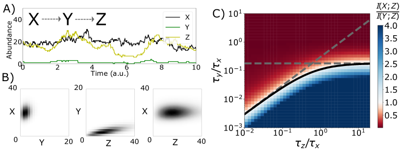
Figure 1: The stationary state distributions of biochemical cascades do not follow the data-processing inequality. A) Example time trace of the linear cascade defined in Eq. 1 in which $X$ affects the production of $Y$, which in turn affects the production of $Z$. B) Corresponding stationary state distribution of the molecules. C) Exact numerical simulation results for the mutual information between pairs of variables in the cascade defined by Eq. 1. Blue region indicates the parameter regime in which numerical simulations exhibited $I(X;Z)>I(Y;Z)$ in seeming, but not actual, violation of the data processing inequality. The solid black line indicates the analytical approximation of Eq. LABEL:EQ:_XZ_YZ_Correlation_Inequality to determine the boundary at which $I(X;Z)=I(Y;Z)$. Dashed grey lines indicate necessary conditions on time-scales that can be interpreted intuitively. Violations occur when $\tau_{y}\ll\tau_{x},\tau_{z}$. Data correspond to simulations of Eq. 1 with $\langle x\rangle=\langle z\rangle=20,\langle y\rangle=2$, which corresponds to a process with a noisy intermediate such that $\eta_{y}^{\text{int}}\gg\eta_{x}^{\text{int}}$. Numerical simulations for other intrinsic noise regimes show similar behaviour, see SI.

Results

Mutual information is non-monotonic along biochemical cascades

To analyze mutual information in biochemical signalling we consider the following stochastic process in which three components $X,Y,Z$ form a linear cascade

$$\begin{array}[]{rcl}x&\xrightarrow{\mathmakebox{\lambda}}&x+1\\ x&\xrightarrow{\mathmakebox{x/\tau_{x}}}&x-1\end{array}\hskip 8.0pt\begin{array}[]{rcl}y&\xrightarrow{\mathmakebox{\alpha\hskip 0.70004ptx}}&y+1\\ y&\xrightarrow{\mathmakebox{y/\tau_{y}}}&y-1\end{array}\hskip 8.0pt\begin{array}[]{rcl}z&\xrightarrow{\mathmakebox{\beta y}}&z+1\\ z&\xrightarrow{\mathmakebox{z/\tau_{z}}}&z-1\end{array}\hskip 3.0pt.$$ (1)

Here, variables linearly affect the production of the next downstream and each component undergoes first order degradation with respective average lifetimes $\tau_{x},\tau_{y},\tau_{z}$.

The (co)variances between components of this generic regulatory cascade have been analyzed previously [22]. Here, we consider the joint stationary state distribution of the components $P_{\text{ss}}(x,y,z)$ and determine the mutual information between pairs of components, defined as [23]

$$I(X;Y):=\sum_{x,y}P_{\text{ss}}(x,y)\log_{2}\left(\frac{P_{\text{ss}}(x,y)}{P_{\text{ss}}(x)P_{\text{ss}}(y)}\right),$$

and analogously for any other pair.

The mutual information between components in a Markov chain is constrained by the data processing inequality [8] which implies

$$I(X;Z) \leq I(Y;Z)$$ (2)

$$I(X;Z) \leq I(X;Y).$$ (3)

This pair of inequalities quantifies how information can only be lost along Markov chains and once information is lost it cannot be recovered through processing. However, the premise of the data processing inequality is that $X,Y,Z$ form a Markov chain, which the variables in the stochastic process Eq. 1 do not.

The biochemical cascade defined in Eq. 1 is memoryless such that its future evolution depends only on the current state but not its history. However, the random variables that correspond to the numbers of molecules in the above biochemical reaction cascade do not form a Markov chain with respect to each other. Even though the variables form an ordered causal relation $X\rightarrow Y\rightarrow Z$ their dynamics are not conditionally independent, i.e., the stationary state probability distributions do not generally satisfy $P(X,Y,Z)=P(X)P(Y|X)P(Z|Y)$ [13, 14, 15].

While this lack of conditional independence might look surprising (and has in fact been mistakenly assumed in related processes [16, 17, 18, 19]), it intuitively follows because the system is a dynamically varying stochastic process rather than a cascade of static random variables. For such stochastic processes the variable trajectories $x(t),y(t),z(t)$ become conditionally independent only when conditioned on the entire history of upstream variables [24, 25, 26, 27].

We first analyze under which conditions the inequality of Eq. 2 will be violated by the stationary state probability distributions of simple biochemical cascades. Exact simulations [28] of the system defined by Eq. 1 show that for any molecular abundance levels, Eq. 2 was violated in the regime when $\tau_{z}/\tau_{x}$ is large and $\tau_{y}/\tau_{x}$ is small as indicated by the blue region in Fig. 1B. In this regime the mutual information between the distantly connected components $X$ and $Z$ significantly exceeds the mutual information between the directly connected $Y$ and $Z$. See SI for numerical simulation results for abundances other than those of Fig. 1B.

To understand the above time-scale dependence, we complement our exact numerical analysis of mutual information with analytical approximations. For multivariate Gaussians, the mutual information between components is related to their correlation through $I(X;Y)=-\log_{2}(1-\rho_{xy}^{2})/2$. When stationary state distributions are approximately Gaussian, we can thus estimate the mutual information between components from their correlations, which can be exactly determined from the system’s chemical master equation, see Appendix A.

Following this approach yields the following (approximate) necessary and sufficient condition to violate Eq. 2.

$$\begin{split}&1+\frac{\tau_{y}}{\tau_{z}}\left(1+\frac{\eta_{y}^{\text{int}}}{\eta_{x}^{\text{int}}}\left(1+\frac{\tau_{y}}{\tau_{x}}\right)\right)\left(1+\frac{\tau_{z}}{\tau_{x}}\right)\\ &\leq\left(1+\frac{\tau_{y}}{\tau_{z}}\right)\left(\frac{\eta_{y}^{\text{int}}}{\eta_{x}^{\text{int}}}+\left(1+\frac{\tau_{y}}{\tau_{x}}\right)^{-1}\right)^{1/2}\end{split}\quad,$$ (4)

for intrinsic noise terms

$$\eta_{x}^{\text{int}}:=\frac{1}{\langle x\rangle},\quad\eta_{y}^{\text{int}}:=\frac{1}{\langle y\rangle},\quad\eta_{z}^{\text{int}}:=\frac{1}{\langle z\rangle}.$$ (5)

Here, and throughout angular brackets denote stationary state averages.

In Fig. 1C, the black line indicates the boundary defined by Eq. LABEL:EQ:_XZ_YZ_Correlation_Inequality which agrees well with the numerical solutions for the cascade defined in Eq. 1 with abundances $\langle x\rangle=\langle z\rangle=20,\langle y\rangle=2$ such that $\eta_{y}^{\text{int}}/\eta_{x}^{\text{int}}=10$. The analytical approximation also accurately describes systems with different intrinsic noise ratios where the average abundances of all molecules are larger than one molecule, see SI.

The analytical condition of Eq. LABEL:EQ:_XZ_YZ_Correlation_Inequality can be intuitively understood in the regimes in which $\tau_{z}$ is much slower or much faster than $\tau_{x}$.

When $\tau_{z}\ll\tau_{x}$ the inequality asymptotically becomes

$$\sqrt{1+\frac{\eta_{y}^{\text{int}}}{\eta_{x}^{\text{int}}}}\leq\frac{\tau_{z}}{\tau_{y}},$$ (6)

as long as $\tau_{y}\ll\tau_{x}$, see Appendix A.2. Eq. 6 is indicated by the diagonal line of Fig. 1.

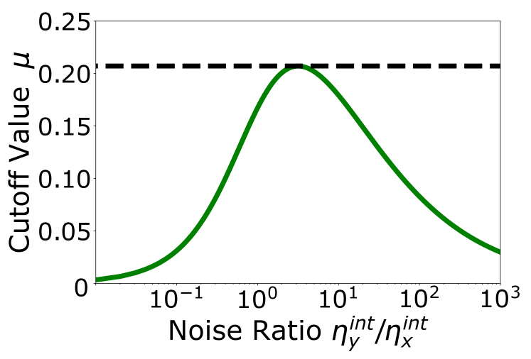
When $\tau_{z}\gg\tau_{x}$ the boundary asymptotically becomes a simple cutoff $\tau_{y}/\tau_{x}\lesssim\mu$ where $\mu$ is the root of a quintic polynomial in $\eta_{y}^{\text{int}}/\eta_{x}^{\text{int}}$, see Appendix A.2. While the root is not analytically accessible we can determine it numerically, see Fig. 2. The cutoff $\mu$ attains its maximum value

$$\mu^{*}=\frac{\sqrt{2}-1}{2}\approx 0.2071,$$ (7)

when $\eta_{x}^{\text{int}}=(6-2\sqrt{2})\eta_{y}^{\text{int}}$, see Fig. 2, suggesting that regardless of any other system details, violations of Eq. 2 cannot not be observed when the lifetime of the intermediate variable is larger than one fifth of the input variable.

These asymptotic behaviours of Eq. LABEL:EQ:_XZ_YZ_Correlation_Inequality translate in a pair of necessary conditions on the time-scales, see grey dashed lines in Fig. 1C. The mutual information between components along a linear cascade is thus expected to violate Eq. 2 when the intermediate component $Y$ is significantly faster than both $X$ and $Z$.

Figure 2: Analytical approximations predict that Eq. 2 will not be violated in cascades with a slow intermediate. Eq. LABEL:EQ:_XZ_YZ_Correlation_Inequality predicts that violating Eq. 2 requires $\tau_{y}/\tau_{x}<\mu$ where the parameter $\mu$ depends on the noise ratio $\eta_{y}^{\text{int}}/\eta_{x}^{\text{int}}$. Violations become impossible in both limits of the noise ratio. Dashed line indicates the analytically determined maximum which corresponds to the largest value of $\tau_{y}/\tau_{x}$ for which we can expect violations of Eq. 2 regardless of any other system details. We thus do not expect violations in cascades with intermediate variables $Y$ that are slow compared to $X$.

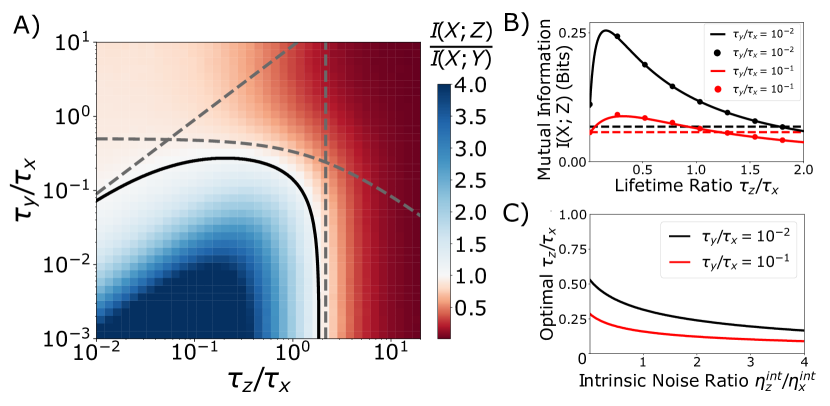
Figure 3: Mutual information can increase along a biochemical cascade. Exact numerical simulation results for the mutual information between pairs of variables in the cascade defined by Eq. 1. Blue region indicates the parameter regime in which $I(X;Z)>I(X;Y)$ corresponding to $\tau_{x}\gg\tau_{y},\tau_{z}$. The solid black line indicates the analytical approximation of Eq. 8 to determine the boundary at which $I(X;Z)=I(X;Y)$. Dashed grey lines indicate the simpler necessary but not sufficient conditions on parameters for violations to occur, described by Eqs. 9 –11. Data corresponds to simulations with same parameters as Fig. 1. B) Plotting the mutual information $I(X;Z)$ as a function of $\tau_{z}/\tau_{x}$ reveals there exists a critical value of $\tau_{z}^{*}/\tau_{x}$ for which $I(X;Z)$ is maximized, as shown by the solid line (the analytical approximation) as well as dots (simulation data), which can both lie above the dashed line ($I(X;Y)$ from simulations) for sufficiently small $\tau_{z}/\tau_{x}$. This occurs because when $Z$ is too fast it cannot average out intrinsic fluctuations in $Y$ and when $Z$ is too slow it averages out the variability of the signal $X$. Note, an optimum only exists in certain regimes. Data corresponds to the same parameters as Fig. 1, for which violations of Eq. 3 only occur for $\tau_{y}/\tau_{x}\leq 0.5$. C) The $\tau_{z}/\tau_{x}$ ratio that maximizes $I(X;Z)$ is a decreasing function of the ratio $\eta_{z}^{\text{int}}/\eta_{x}^{\text{int}}$, see Appendix A.1.

The above results show how in biochemical cascades, the mutual information between the last component and their upstream components can be non-monotonic, i.e., components that are further removed from the final read-out can have larger mutual information with compared to those closer connected to the final component. Next, we consider the complementary question when an apparent “loss of information” in the first step will be recovered through an additional step in the cascade, i.e., we analyze the conditions under which inequality Eq. 3 is violated.

Previous work [20, 21] established that this inequality can be violated when the signalling timescale is long lived compared to the downstream components, which have equal lifetimes and increasing averages along the cascade. Through numerical simulations over a wide range of parameters, we find that violations for any set of intrinsic noise ratios depend on the relative time-scales of the components as indicated in Fig. 3A). Changing the intrinsic noise ratios by adjusting average abundances significantly changes these results, with no violations occurring for some intrinsic noise ratios, see SI.

To understand this dependence we derive (approximate) analytical conditions to violate Eq. 3. Following the same approach as above, we translate the exact (co)variance solutions for Eq. 1 into the following necessary and sufficient condition to violate Eq. 3

$$\left(\frac{1}{1+\mfrac{\tau_{z}}{\tau_{y}}}+\frac{1}{1+\mfrac{\tau_{y}}{\tau_{z}}}\frac{1}{1+\mfrac{\tau_{z}}{\tau_{x}}}\right)+\frac{\eta_{z}^{\text{int}}}{\eta_{x}^{\text{int}}}\left(1+\frac{\tau_{z}}{\tau_{x}}\right)^{2}$$

$$\leq\frac{\eta_{y}^{\text{int}}}{\eta_{x}^{\text{int}}}\left(1-\frac{\left(1+\mfrac{\tau_{z}}{\tau_{x}}\right)^{2}}{1+\mfrac{\tau_{z}}{\tau_{y}}}\right)+\frac{1}{1+\mfrac{\tau_{y}}{\tau_{x}}}$$ (8)

The boundary defined by Eq. 8 agrees well with the exact numerical results for a system with noise ratios $\eta_{y}^{\text{int}}/\eta_{x}^{\text{int}}=10$ and $\eta_{z}^{\text{int}}=\eta_{x}^{\text{int}}$, as indicated by the solid black line in Fig. 3A.

To intuitively understand the condition of Eq. 3 we first consider the maximum $\tau_{z}/\tau_{x}$ above which violations become impossible. The exact cut-off value depends on both noise ratios (see SI) but is itself bounded by

$$\frac{\tau_{z}}{\tau_{x}}\leq\sqrt{\frac{\eta_{y}^{\text{int}}}{\eta_{z}^{\text{int}}}}-1,$$ (9)

indicated by the vertical (solid) grey line in Fig. 3. Note, this implies that violating Eq. 3 is impossible when the read-out-variable is noisier than the intermediate, i.e., when $\eta_{z}^{\text{int}}>\eta_{y}^{\text{int}}$.

By considering the regime in which $\tau_{z},\tau_{y}\ll\tau_{x}$, we obtain the following necessary condition

$$\frac{\tau_{y}}{\tau_{z}}\leq\mfrac{\eta_{y}^{\text{int}}}{\eta_{z}^{\text{int}}}-1.$$ (10)

This inequality illustrates that the read-out variable $Z$ must become longer lived the closer its intrinsic noise gets to that of the intermediate in order for violations to occur. The condition of Eq. 10 is indicated by the diagonal dashed grey line in Fig. 3.

Finally, we consider the limit in which the intermediate component is far noisier than the others, i.e., $\eta_{y}^{\text{int}}\gg\eta_{x}^{\text{int}},\eta_{z}^{\text{int}}$. In this regime, Eq. 3 becomes independent of the noise ratios and constrains the time-scales through

$$\frac{\tau_{y}}{\tau_{x}}\leq\frac{1}{2}\left(1+\frac{\tau_{z}}{2\tau_{x}}\right)^{-1}.$$ (11)

indicated by the curved dashed grey line in Fig. 3. Note, Eq. 11 puts an absolute upper limit on the lifetime of the intermediate variable. For violations of Eq. 3 to occur, the input variable must be at least two times longer lived than the intermediate regardless of any other system parameters. Eqs. 9, 10, and 11 are derived in Appendix  A.2.

While the above intuitive conditions are necessary but not sufficient they describe the region of violations quite well, as indicated by the dashed grey lines in Fig. 3. In general, violations of Eq. 3 are expected to occur when the intermediate component $Y$ has significantly more noise than the read-out variable $Z$, and the intermediate is the fastest component in the cascade.

Note, that combining the conditions of Eqs. LABEL:EQ:_XZ_YZ_Correlation_Inequality and 8 shows that the inequalities of Eqs. 2 and 3 can be violated simultaneously. The overlapping blue regions in Figs. 1 and 3 correspond to cascades in which the input signal $X$ is the slowest varying component and the intermediate component $Y$ is significantly faster than the other variables and contains more intrinsic noise than $Z$. In this regime, the mutual information between the components at the end of the cascade is larger than that of either intermediate pair.

To understand how an additional “read-out” variable can increase mutual information it is most intuitive to consider the regime in which the input signal varies on slower time-scales than the lifetime of downstream cellular components, i.e., $\tau_{x}\gg\tau_{y},\tau_{z}$ as is often the case for biological input signals. Under the Gaussian approximation, the mutual information between $X$ and $Y$ in this regime is given by

$$I(X;Y)=\frac{1}{2}\log_{2}\left(1+\frac{\eta_{x}^{\text{int}}}{\eta_{y}^{\text{int}}}\right).$$ (12)

In contrast, the mutual information between $X$ and $Z$ is given by

$$\begin{split}I(X;Z)&=\frac{1}{2}\log_{2}\left(1+\frac{\eta_{x}^{\text{int}}}{\eta_{z}^{\text{int}}}\frac{1}{1+\mfrac{\eta_{y}^{\text{int}}}{\eta_{z}^{\text{int}}}\mfrac{1}{1+\frac{\tau_{z}}{\tau_{y}}}}\right).\end{split}$$ (13)

Whereas the magnitude of $I(X;Y)$ is limited by $\eta_{x}^{\text{int}}/\eta_{y}^{\text{int}}$, $I(X;Z)$ is ultimately limited by the ratio of $\eta_{x}^{\text{int}}/\eta_{z}^{\text{int}}$ when $Z$ becomes infinitely slow. If the intrinsic noise of $Z$ is smaller than that of $Y$ the additional read-out step thus performs time-averaging that effectively replaces the intrinsic noise of $Y$ with that of $Z$. How much time-averaging is needed to violate Eq. 3 depends on the ratio of intrinsic noises as given by Eq. 10.

This suggests the increase in mutual information across more distant variables in a cascade occurs because the intrinsic noise of intermediates are not transmitted through the cascade. By filtering out the intrinsic noise of the intermediate, the variability of $Z$ only contains contributions from $X$ and its own intrinsic noise $\eta_{z}^{\text{int}}$, which can be less than $\eta_{y}^{\text{int}}$.

In our cascade, the filtering is done via time averaging, similar to the well known result from studying two variable cascades where fast fluctuations are not passed down to longer-lived downstream components [29, 22, 10, 30]. Time-averaging to improve estimation is not a novel concept in biology, eg. in bacterial sensing where it is known that increasing time alloted before making a decision improves the accuracy by allowing for more samples [31].

Optimal time-scale for maximizing mutual information

The above results show that adding a component to a biochemical cascade can increase the mutual information between the last component and the upstream input. Next, we determine the optimal time-scale over which the additional variable $Z$ should average out fluctuations to maximize $I(X;Z)$.

For distributions that are approximately Gaussian, we find for the ideal read-out variable with $\eta_{z}^{\text{int}}=0$ the optimal time-scale is given by

$$\begin{split}\tau_{z}^{*}=\tau_{x}&\sqrt{\frac{\mfrac{\tau_{y}}{\tau_{x}}-2\left(\mfrac{\tau_{y}}{\tau_{x}}\right)^{3}-\left(\mfrac{\tau_{y}}{\tau_{x}}\right)^{2}\left(1+2\mfrac{\eta_{x}^{\text{int}}}{\eta_{y}^{\text{int}}}\right)}{\left(1+\mfrac{\tau_{y}}{\tau_{x}}\right)\left(\mfrac{\eta_{x}^{\text{int}}}{\eta_{y}^{\text{int}}}+\mfrac{\tau_{y}}{\tau_{x}}\right)}}\end{split}\quad.$$ (14)

The existence of this optimum can be intuitively understood because in the limit of $\tau_{z}\to\infty$, $Z$ averages out both intrinsic fluctuations from the intermediate as well as the signal, see Fig. 3B. For read-out variables with finite noise, the optimal time-scale $\tau_{z}^{*}$ slowly decreases as $\eta_{z}^{\text{int}}$ increases until ultimately violations of Eq. 3 are no longer possible for any value of $\tau_{z}$, see Fig. 3C and Appendix A.1.

On-off upstream

Instead of a Poissonian input signal to our two-step cascade, we next consider a two-state input, e.g., motivated by a single receptor that is in a bound/unbound state, or by a gene stochastically switching between two transcriptional states, resulting in the following cascade in which $\lambda$ stochastically switches

$$\begin{gathered}\lambda_{\text{off}}\xrightleftharpoons[k_{\mathrm{off}}]{\mathmakebox{k_{\mathrm{on}}}}\lambda_{\text{on}}\\ \begin{array}[]{rcl}y&\xrightarrow{\mathmakebox{\alpha\hskip 0.70004pt\lambda}}&y+1\\ y&\xrightarrow{\mathmakebox{y/\tau_{y}}}&y-1\end{array}\hskip 8.0pt\begin{array}[]{rcl}z&\xrightarrow{\mathmakebox{\beta y}}&z+1\\ z&\xrightarrow{\mathmakebox{z/\tau_{z}}}&z-1\end{array}\hskip 3.0pt.\end{gathered}$$ (15)

Figure 4: On-off upstream signals violate of the data-processing inequality with Gaussian approximations making accurate qualitative but not quantitative predictions. A) Comparing exact numerical simulations with analytical results from solving the chemical master equation and applying the Gaussian approximation for the cascade defined by Eqs. 1, 15. Correlation coefficients are exactly predicted by the linear noise approximation (LNA) because all rates are linear. Mutual information is only approximately predicted by Gaussian approximations. Data corresponds to a cascade with $\langle y\rangle=2,\langle z\rangle=20,\tau_{y}/\tau_{\lambda}=0.1$ and $P_{\text{on}}=0.5$. B) Exact numerical simulations show the Gaussian approximation (black line) no longer quantitatively predicts the region of violations, but qualitative time-scale features are accurately characterized, i.e., violations occur for Eq. 2 when the intermediate $Y$ is significantly faster than both $X,Z$, and violations for Eq. 3 occur when the signal timescales are longer lived than all other components. Same parameters as panel (A).

Exact numerical simulations of Eq. 15 show that Eqs. 2, 3 are also violated in this strongly non-Gaussian regime, see Fig. 4C. Note, the stochastic switching process of Eq. 15 yields identical mathematical forms for the covariances and correlation coefficients as the original model given by Eq. 1 with the only difference that intrinsic noise of the input signal is now given by

$$\eta_{\lambda}^{\text{int}}=\frac{1-P_{\text{on}}}{P_{\text{on}}}.$$ (22)

where $P_{\text{on}}$ is the fraction of time the gene spends in the on-state, and the signal timescale is $\tau_{\lambda}=1/(k_{\text{on}}+k_{\text{off}})$. As far as correlation coefficients are concerned, the systems behave identically and can be exactly solved analytically using the standard linear noise approach [29]. It is the Gaussian approximation for the mutual information that is no longer exact, see Fig. 4A.

While the behaviour is now quantitatively different from the simple analytical approximation, the qualitative behaviour remains: Violations for Eq. 2 occur when the intermediate $Y$ is significantly faster than both $X,Z$, and violations for Eq. 3 occur when the signal timescales are longer lived than all other components.

Differences between the Gaussian approximation and the exact simulation data also become apparent for the original system Eq. 1 when at least one of the average abundances become smaller than one, see SI.

Other types of biochemical cascades

In the previous section we showed that mutual information can increase along the cascade defined in Eq. 1. Next, we analyze mutual information along more complex cascades to analyze the effect of molecular conversion events, more components, or proofreading steps.

.0.1 Cascades with molecular conversion events

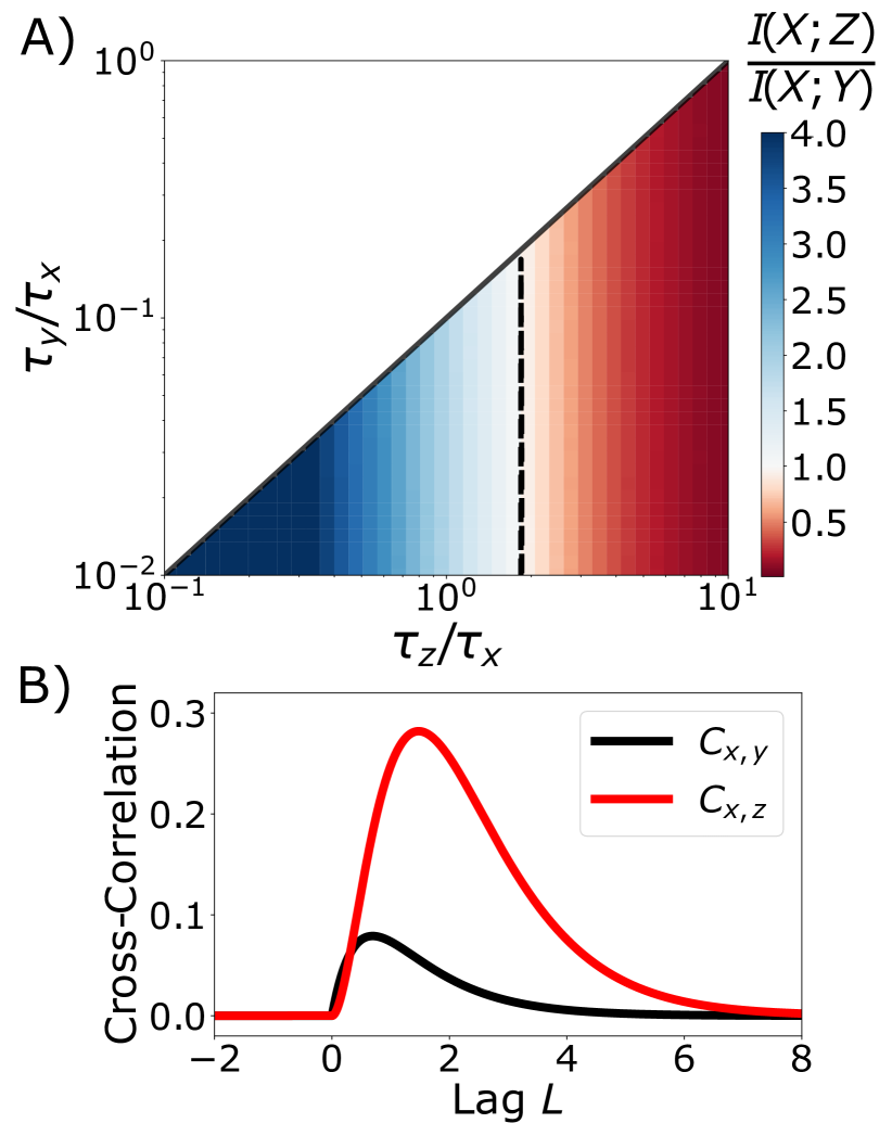
Figure 5: Cascades with conversion events also exhibit mutual information reversal that depends on the time-scales. A) Exact numerical simulation results for the model defined by Eq. 1 and Eq. 23 where $Y$ molecules are born through catalytic production and $Z$ molecules only through conversion events. Data correspond to cascade with $\langle x\rangle=\langle z\rangle=20,\langle y\rangle=2$. Cascades with conversion reactions and fixed averages are constrained in molecular lifetimes, resulting in the triangular accessible region. The (almost) vertical black dashed line corresponds to the Gaussian prediction for $I(X;Z)=I(X;Y)$ which closely matches the numerical data. B) Temporal cross-correlations between components in a linear cascade in which $X$ converts into $Y$ which converts into $Z$. Lag is measured in units of $\tau_{x}$. For zero lag the cross-correlation is zero because the steady state distributions are statistically independent. The causal connection between components only becomes apparent for non-zero lags. Data correspond to same cascade as in panel (A) with lifetimes $\tau_{x}=1,\tau_{y}=0.5,\tau_{z}=0.8$.

In the cascade defined by Eq. 1 the levels of one molecule set the production rate of another. However, in biochemical cascades one molecule might convert into another, for example, through conformational changes, which introduces chemical reactions that simultaneously change the levels of two molecular species. For example, we first consider the case where the intermediate variable $Y$ converts into the final read-out variable $Z$ by replacing the production reaction of $Z$ and the degradation reaction of $Y$ in Eq. 1 with

$$\begin{array}[]{rcl}(y,z)&\xrightarrow{\mathmakebox{\beta_{1}\hskip 0.70004pty}}&(y-1,z+1)\\ y&\xrightarrow{\mathmakebox{\beta_{2}\hskip 0.70004pty}}&y-1\end{array}\hskip 3.0pt,$$ (23)

with the lifetime of the intermediate component given by $\tau_{y}=1/\left(\beta_{1}+\beta_{2}\right)$.

Exact numerical simulations of this cascade show that Eq. 3 can be violated over a large range of timescales, see Fig. 5A. This occurs because $Z$ no longer inherits intrinsic noise from $Y$, see Appendix B. This is most easily seen in the limit where $\tau_{x}\gg\tau_{y},\tau_{z}$, where the Gaussian approximation gives

$$I(X;Z)=\frac{1}{2}\log_{2}\bigg{(}1+\frac{\eta_{x}^{\text{int}}}{\eta_{z}^{\text{int}}}\bigg{)}\quad.$$ (26)

Compared to Eq. 13, which required $\tau_{z}\gg\tau_{y}$ for the read-out variable to remove the effect of intrinsic noise from the intermediate, in a cascade in which $Y$ converts into $Z$ the final read out removes the intermediate noise at all lifetimes. $I(X;Z)$ is always larger than in the case without conversions, which explains why violations occur over a wider range of time-scales as $I(X;Y)$ has remained unchanged, see Appendix B.

In the above cascade with a final conversion event, $I(X;Z)$ decreases monotonically with $\tau_{z}$. Thus the optimal $\tau_{z}^{*}=0$ and there is no advantage of time-averaging with larger $\tau_{z}$ when the intermediate noise is already filtered out via the conversion reaction, see Appendix B.

Next, we consider the case where $Y$ but not $Z$ molecules are made in conversion events, i.e., $X$ turns into $Y$ but $Z$ is made catalytically. This corresponds to replacing the $Y$ production in Eq. 1 with

$$\begin{array}[]{rcl}(x,y)&\xrightarrow{\mathmakebox{\alpha_{1}\hskip 0.70004ptx}}&(x-1,y+1)\\ x&\xrightarrow{\mathmakebox{\alpha_{2}\hskip 0.70004ptx}}&x-1\end{array}\hskip 3.0pt,$$ (27)

where the lifetime of the signal is now $\tau_{x}=1/\left(\alpha_{1}+\alpha_{2}\right)$.

In this cascade the stationary state distribution takes the form $P(x,y,z)=P(x)\times P(y,z)$ where $P(x)$ is a Poisson distribution, and $P(y,z)$ is the stationary state distribution of a system in which $Y$ is made at a constant rate, see Appendix B. The initial conversion event thus makes the downstream components statistically independent of the signal and there is no mutual information between $X$ and its downstream variables. The stationary state distribution $P(y,z)$ for the this two-step cascade (which is commonly used to model mRNA-protein dynamics) has been explicitly computed [32].

To illustrate why the concept of statistical independence can be dramatically misleading when applied to stationary state distributions of stochastic processes we consider the case of a conversion cascade in which both $Y$ and $Z$ molecules are made in conversion events. This cascade belongs to a family of reaction networks for which the stationary state distribution is the product of three independent Poisson distributions [33, 34], which implies that the mutual information between any pair of variables is zero [5].

The physical dependence of these causally connected variables is not apparent in the statistical independence of the joint steady-state distributions because steady-state distributions consider molecular levels at the same time. The interactions between the components only become apparent when considering the cross-correlation

$$C_{i,j}(L)=\frac{\langle x_{i}(t)x_{j}(t+L)\rangle-\langle x_{i}(t)\rangle\langle x_{j}(t)\rangle}{\sqrt{\text{Var}(i)\text{Var}(j)}}$$ (30)

for non-zero lags, see Fig. 5B and Appendix B. This highlights how intuition from static random variables can be misleading when applied to stationary state distributions of biochemical reaction networks.

When considering the stationary-state distribution, an initial conversion event will seemingly disconnect the input variable from the any downstream variable regardless of the length of the cascade. Consider the following general linear cascade $X_{1}\rightarrow X_{2}\rightarrow...\rightarrow X_{k}$, where $X_{1}$ is produced at a constant rate, and all molecules undergo first order degradation reactions while arrows denote first order production rates that can be a molecular conversion reactions or simple one component setting the production rate of the next. For all such cascades the normalized covariance between components monotonically decreases over the cascade according to

$$\frac{\mathrm{Cov}(x_{1},x_{k})}{\langle x_{1}\rangle\langle x_{k}\rangle}=\frac{\mathrm{Cov}(x_{1},x_{k-1})}{\langle x_{1}\rangle\langle x_{k-1}\rangle}\frac{1}{1+\mfrac{\tau_{k}}{\tau_{1}}}$$ (31)

where $\tau_{1},\tau_{k}$ denote the average lifetimes of the first and $k^{\mathrm{th}}$ molecules in the chain. The above formula holds for $k\geq 3$, see Appendix B. A cascade that starts with a conversion event thus has $\text{Cov}(x_{1},x_{k})=0$ for all $k\geq 2$.

.0.2 Longer cascades

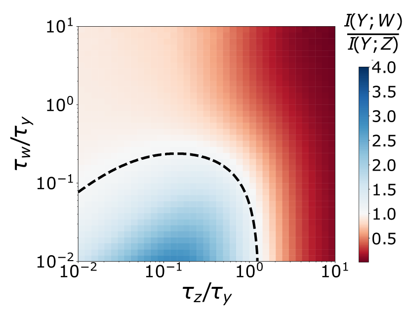
Figure 6: Non-monotonic behavior of mutual information in longer linear cascades. Exact numerical simulation results for the ratio of mutual information $I(Y;W)/I(Y;Z)$ for the model defined in Eqs. 1 and 32 reveals that $I(Y;W)>I(Y;Z)$ can occur. This shows that mutual information can increase even when the upstream signal is no longer a Poissonian variable. The graph was generated for $\langle x\rangle=0.5,\langle y\rangle=\langle w\rangle=20,\langle z\rangle=2,\tau_{x}=0.1,\tau_{y}=1$.

Arguably, the analysis of the two-step cascade of Eq. 1 corresponded to a special case in which all tested inequalities involved the mutual information between a Poisson variable and a downstream component. We thus next analyze the mutual information between the second, third, and forth component in a three-step cascade. We consider the dynamics of Eq. 1 with the following additional reactions

$$\begin{array}[]{rcl}w&\xrightarrow{\mathmakebox{\gamma z}}&w+1\\ w&\xrightarrow{\mathmakebox{w/\tau_{w}}}&w-1\end{array}\quad.$$ (32)

Numerical simulations show that it is again possible for mutual information to be larger between more distant variables. The parameters for this regime are similar to the original two step cascade, where the intrinsic noise of the intermediate (now $Z$), and the lifetimes of downstream components must be small compared to the timescale of the upstream variability.

This cascade also allows us to study the behaviour of mutual information over multiple intermediates, for which it has been previously shown that the mutual information can increase for certain parameters [20, 21]. Our analytical approximation suggests such violations occur because Eq. 13 generalizes, meaning the noise of multiple intermediates is not passed down depending on the relative lifetimes of the molecules involved. For the approximation results for mutual information, see Appendix C.

.0.3 Kinetic proofreading

Next, we consider kinetic proofreading [35, 36], which can enhance the response of cells to different ligand occupancies and is commonly believed to allow cells to better distinguish between two ligands. However, recent work has shown that the increased average differences come at the cost of increased intrinsic noise which generally worsens the ability to distinguish between different ligands [37].

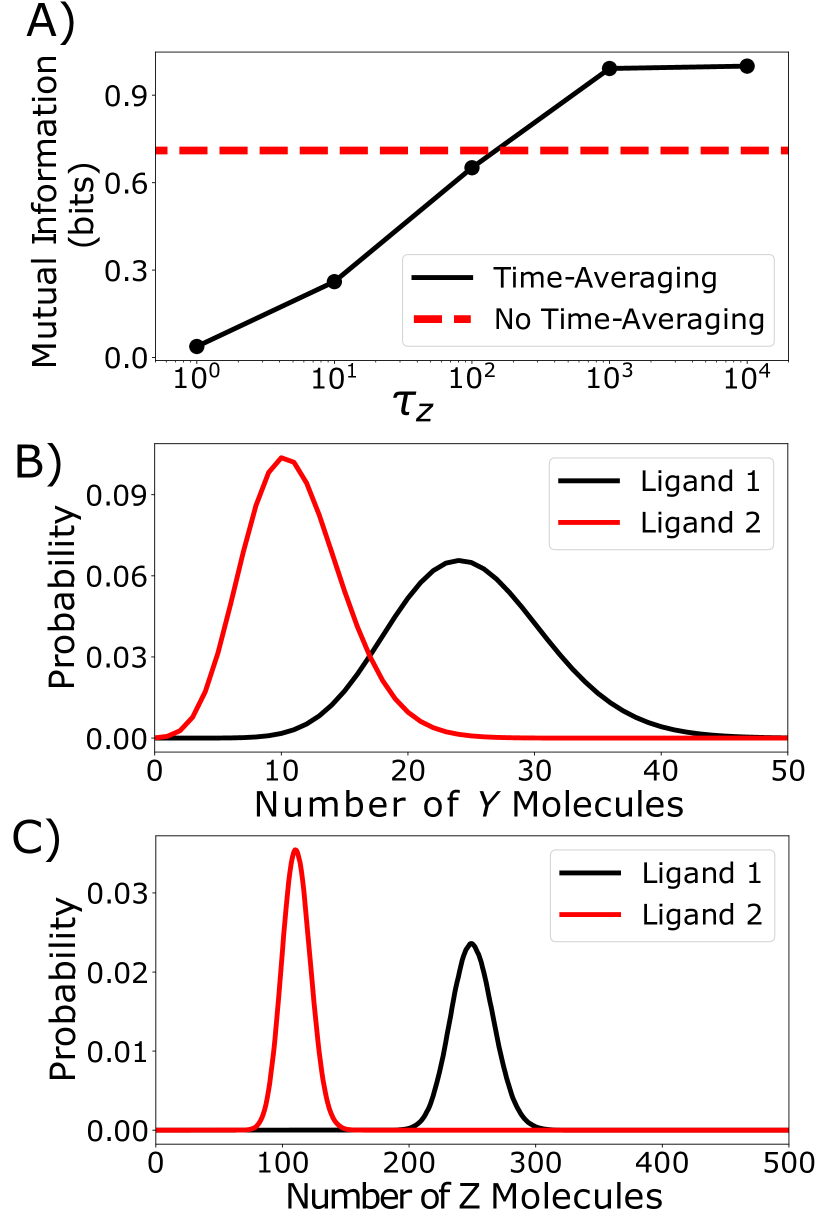
Figure 7: Time-averaging can alleviate the mutual information decreasing effect of kinetic proofreading. A) Simulation results for the simple kinetic proofreading model defined in the main text. Mutual information between the receptor output and the ligand dependent $I(k_{\text{off}},Y)$ (dashed red line) can be increased by adding an extra variable that time-averages the receptor output, $I(k_{\text{off}},Z)$ (solid black line). B) The probability distribution of the receptor output. Although different ligands result in different output averages, intrinsic noise causes their distributions to overlap. C) Time-averaging effectively reduces the impact of intrinsic noise in $Y$ as illustrated by the much more separated probability distribution of the final read-out variable $Z$.

The effect of increased intrinsic noise in kinetic proofreading has been quantified through computing mutual information between ligand affinity and receptor output [37]. We analyze the mutual information in the following model: ligands bind at a diffusion limited rate $k_{\text{on}}$, advance from the initial bound state to subsequent proofreading states at a rate $k_{f}$, and unbind from any state with a ligand dependent rate $k_{\text{off}}$. In the final bound state the receptor produces downstream signalling molecules $Y$ at a rate $k_{p}$. The unbinding rate $k_{\text{off}}$ depends on the ligand affinity while all other are assumed to be ligand independent. Considering two different ligands we consider the mutual information between downstream components and the unbinding rate $k_{\text{off}}$ that takes two different values with equal probability on a time-scale much slower than $\tau_{y},\tau_{z}$.

The results of the previous sections suggest that the effect of increased intrinsic noise in proofreading can be removed through time-averaging with an additional reaction step $Y\rightarrow Z$, when $\tau_{z}>\tau_{y}$. Indeed, numerical simulation results confirm this intuition for a single receptor with two potential ligands of different affinities such that $I(k_{\text{off}},Z)$ is larger than $I(k_{\text{off}},Y)$, see Fig. 7A.

This result can be intuitively understood by looking at the probability distribution of output molecules. Although proofreading enhances the differences in average output associated with each ligand type, intrinsic noise can cause the resulting output distributions to overlap [37], see Fig. 7B. Adding an additional processing step with time-averaging can reduce the impact of intrinsic noise, see Fig. 7C. Intrinsic noise can also be reduced by increasing the lifetime of the output molecule $Y$ instead of adding an additional processing step. However, both methods of increasing the mutual information come at the expense of slowing down the system response to changes in ligand concentration highlighting a general speed-accuracy trade-off in sensing systems [38].

Discussion

Our results establish the conditions under which the data-processing inequality is violated by stationary state distributions of molecular abundances in a biochemical reaction cascade. By systemically varying parameters in Gillespie simulations we obtained exact (within numerical error) steady state probability distribution for various cascade models. We complemented these exact numerical simulations with approximate analytical expressions to provide insight into the behaviour over all parameters.

The analytical conditions show that violations generally reflect a fast intermediate variable that is noisy compared to the other components. In biology, the timescale of the signal is often much longer than the lifetimes of the downstream components. Our analysis shows that this is precisely the regime where one can observe violations in the data-processing inequality.

Our analytical expressions were obtained by approximating the steady state distribution as multivariate Gaussian distribution similar to previous work [5, 17, 39, 18, 19]. Direct comparison showed that the mutual information between components in our cascades was well described by Gaussian approximations as long as average abundances are not lower than two molecules.

These results re-emphasize that the mutual information between stationary state distributions of cellular abundances is not a measure of information flow. This mutual information is a statistical measure of similarity between the distributions of molecular levels which can be increased by post-processing. Mutual information between stationary state distributions is thus of limited utility for understanding complex signalling processes through partial observations.

Author Contributions

RF derived the analytical results and performed the numerical simulations. RF and AH wrote the article.

Declaration of Interests

The authors declare that they do not have any competing interests.

Appendix

A Two-step cascade correlations and mutual information

For chemical reaction systems with linear rates all moments can be exactly derived from the chemical master equation. In particular, the matrix of normalized (co)variances $\eta_{ij}:=\mathrm{Cov}(x_{i},x_{j})/(\langle x_{i}\rangle\langle x_{j}\rangle)$ satisfies the Lyapunov equation [40, 29, 22, 41]

$$M\eta+(M\eta)^{T}+D=0\quad,$$ (35)

where $M$ and $D$ for the stochastic reaction system defined by Eq. 1 are given by

$$M =\left(\begin{array}[]{ccc}-\dfrac{1}{\tau_{x}}&0&0\\ \dfrac{1}{\tau_{y}}&-\dfrac{1}{\tau_{y}}&0\\ 0&\dfrac{1}{\tau_{z}}&-\dfrac{1}{\tau_{z}}\\ \end{array}\right),$$ (39)

$$D =\left(\begin{array}[]{ccc}\dfrac{2}{\tau_{x}\langle x\rangle}&0&0\\ 0&\dfrac{2}{\tau_{y}\langle y\rangle}&0\\ 0&0&\dfrac{2}{\tau_{z}\langle z\rangle}\\ \end{array}\right).$$ (43)

Using Eqs. (35,39), one can solve for the following (normalized) covariances

$$\begin{split}&\eta_{xx}=\frac{1}{\langle x\rangle},\hskip 70.0pt\eta_{xy}=\frac{1}{\langle x\rangle}\frac{1}{1+\mfrac{\tau_{y}}{\tau_{x}}}\\ &\eta_{yy}=\frac{1}{\langle y\rangle}+\frac{1}{\langle x\rangle}\frac{1}{1+\mfrac{\tau_{y}}{\tau_{x}}},\quad\eta_{xz}=\frac{1}{\langle x\rangle}\frac{1}{1+\mfrac{\tau_{y}}{\tau_{x}}}\frac{1}{1+\mfrac{\tau_{z}}{\tau_{x}}}\\ &\eta_{yz}=\frac{1}{\langle y\rangle}\frac{1}{1+\mfrac{\tau_{z}}{\tau_{y}}}+\frac{1}{\langle x\rangle}\frac{1}{1+\mfrac{\tau_{y}}{\tau_{x}}}\left(\frac{1}{1+\mfrac{\tau_{z}}{\tau_{x}}}\frac{1}{1+\mfrac{\tau_{y}}{\tau_{z}}}+\frac{1}{1+\mfrac{\tau_{z}}{\tau_{y}}}\right)\\ &\eta_{zz}=\frac{1}{\langle z\rangle}+\frac{1}{\langle y\rangle}\frac{1}{1+\mfrac{\tau_{z}}{\tau_{y}}}+\frac{1}{\langle x\rangle}\frac{1}{1+\mfrac{\tau_{y}}{\tau_{x}}}\\ &\hskip 30.0pt\times\left(\frac{1}{1+\mfrac{\tau_{z}}{\tau_{x}}}\frac{1}{1+\mfrac{\tau_{y}}{\tau_{z}}}+\frac{1}{1+\mfrac{\tau_{z}}{\tau_{y}}}\right).\end{split}$$ (44)

These covariances yield the following correlation coefficients

$$\begin{split}\rho_{xy}=&\frac{1}{1+\mfrac{\tau_{y}}{\tau_{x}}}\left(\frac{1}{\mfrac{\langle x\rangle}{\langle y\rangle}+\frac{1}{1+\mfrac{\tau_{y}}{\tau_{x}}}}\right)^{1/2}\\ \rho_{xz}=&\bigg{(}\frac{1}{1+\mfrac{\tau_{y}}{\tau_{x}}}\bigg{(}\frac{1}{1+\mfrac{\tau_{z}}{\tau_{y}}}+\frac{1}{1+\mfrac{\tau_{y}}{\tau_{z}}}\frac{1}{1+\mfrac{\tau_{z}}{\tau_{x}}}\bigg{)}\\ &+\frac{\langle x\rangle}{\langle z\rangle}+\frac{\langle x\rangle}{\langle y\rangle}\frac{1}{1+\mfrac{\tau_{z}}{\tau_{y}}}\bigg{)}^{-1/2}\times\frac{1}{1+\mfrac{\tau_{y}}{\tau_{x}}}\frac{1}{1+\mfrac{\tau_{z}}{\tau_{x}}}\\ \rho_{yz}=&\bigg{(}\frac{\langle x\rangle}{\langle y\rangle}\frac{1}{1+\mfrac{\tau_{z}}{\tau_{y}}}+\frac{1}{1+\mfrac{\tau_{y}}{\tau_{x}}}\left(\frac{1}{1+\mfrac{\tau_{z}}{\tau_{x}}}\frac{1}{1+\mfrac{\tau_{y}}{\tau_{z}}}+\frac{1}{1+\mfrac{\tau_{z}}{\tau_{y}}}\right)\bigg{)}\\ &\times\bigg{(}\bigg{(}\frac{1}{1+\mfrac{\tau_{y}}{\tau_{x}}}\bigg{(}\frac{1}{1+\mfrac{\tau_{z}}{\tau_{x}}}\frac{1}{1+\mfrac{\tau_{y}}{\tau_{z}}}+\frac{1}{1+\mfrac{\tau_{z}}{\tau_{y}}}\bigg{)}\\ &+\frac{\langle x\rangle}{\langle z\rangle}+\frac{\langle x\rangle}{\langle y\rangle}\frac{1}{1+\mfrac{\tau_{z}}{\tau_{y}}}\bigg{)}\bigg{(}\frac{\langle x\rangle}{\langle y\rangle}+\frac{1}{1+\mfrac{\tau_{y}}{\tau_{x}}}\bigg{)}\bigg{)}^{-1/2}.\end{split}$$ (45)

A.1 Mutual Information

Approximating the stationary state distribution of Eq. 1 as a multivariate Gaussian with the same second order moments allows us to obtain approximate analytic expressions for the mutual information via

$$I(X;Y)=-\frac{1}{2}\log_{2}\bigg{(}1-\rho_{xy}^{2}\bigg{)}.$$ (46)

The expressions obtained from applying Eq. 46 to the correlation coefficients of Eq. 45 lead to the inequalities Eq. LABEL:EQ:_XZ_YZ_Correlation_Inequality and Eq. 8 via elementary algebraic manipulations.

We find this approximation accurately describes the mutual information in our cascade unless average abundances fall below two molecules at which point the discreteness of the distribution becomes apparent, see SI.

To show that the the lifetime ratio $\tau_{z}^{*}/\tau_{x}$ that maximizes the mutual information $I(X;Z)$ is a decreasing function of $\eta_{z}^{\text{int}}/\eta_{x}^{\text{int}}$, note that the mutual information given by Eq. 46 is an increasing function of the correlation coefficient. When $\eta_{z}^{\text{int}}/\eta_{x}^{\text{int}}\rightarrow 0$, the correlation coefficient is given by

$$\begin{split}\rho_{xz}=&\left(\frac{1}{1+\mfrac{\tau_{y}}{\tau_{x}}}\left(\frac{1}{1+\mfrac{\tau_{z}}{\tau_{y}}}+\frac{1}{1+\mfrac{\tau_{y}}{\tau_{z}}}\frac{1}{1+\mfrac{\tau_{z}}{\tau_{x}}}\right)+\frac{\langle x\rangle}{\langle y\rangle}\frac{1}{1+\mfrac{\tau_{z}}{\tau_{y}}}\right)^{-1/2}\\ &\times\frac{1}{1+\mfrac{\tau_{y}}{\tau_{x}}}\frac{1}{1+\mfrac{\tau_{z}}{\tau_{x}}}.\end{split}$$ (47)

for which a nonzero optimal time scale $\tau_{z}^{*}$ (given by Eq. 14) can exist because the denominator can decrease faster with $\tau_{z}$ than the numerator due to the $\langle x\rangle/\langle y\rangle$ term.

When $\eta_{z}^{\text{int}}/\eta_{x}^{\text{int}}\gg\eta_{z}^{\text{int}}/\eta_{x}^{\text{int}},1$, then

$$\begin{split}\rho_{xz}=&\left(\frac{\eta_{x}^{\text{int}}}{\eta_{z}^{\text{int}}}\right)^{1/2}\times\frac{1}{1+\mfrac{\tau_{y}}{\tau_{x}}}\frac{1}{1+\mfrac{\tau_{z}}{\tau_{x}}}\end{split}$$ (48)

for which the optimal time scale is $\tau_{z}^{*}=0$, as the correlation coefficient is a decreasing function of $\tau_{z}$. Increasing $\eta_{z}^{\text{int}}/\eta_{x}^{\text{int}}$ reduces the effect of the $\langle x\rangle/\langle y\rangle$ term monotonically, resulting in smaller optimal $\tau_{z}^{*}$ until eventually $\tau_{z}^{*}=0$ .

A.2 Mutual Information Inequalities

Applying the two limits $\tau_{z},\tau_{y}\ll\tau_{x}$ to Eq. LABEL:EQ:_XZ_YZ_Correlation_Inequality results in

$$\begin{split}1+\frac{\tau_{y}}{\tau_{z}}\left(1+\frac{\eta_{x}^{\text{int}}}{\eta_{y}^{\text{int}}}\right)\leq\left(1+\frac{\tau_{y}}{\tau_{z}}\right)\left(1+\frac{\eta_{x}^{\text{int}}}{\eta_{y}^{\text{int}}}\right)^{1/2}\end{split}\quad,$$ (49)

from which Eq. 6 follows from algebraic manipulations.

The equality of Eq. LABEL:EQ:_XZ_YZ_Correlation_Inequality implies

$$\begin{split}\frac{\tau_{z}}{\tau_{x}}=\frac{-\mfrac{\tau_{y}}{\tau_{x}}\left(1+\mfrac{\eta_{x}^{\text{int}}}{\eta_{y}^{\text{int}}}\left(1+\mfrac{\tau_{y}}{\tau_{x}}\right)-\sqrt{\mfrac{\eta_{x}^{\text{int}}}{\eta_{y}^{\text{int}}}+\left(1+\mfrac{\tau_{y}}{\tau_{x}}\right)^{-1}}\right)}{1+\mfrac{\tau_{y}}{\tau_{x}}\left(1+\mfrac{\eta_{x}^{\text{int}}}{\eta_{y}^{\text{int}}}\left(1+\mfrac{\tau_{y}}{\tau_{x}}\right)\right)-\sqrt{\mfrac{\eta_{x}^{\text{int}}}{\eta_{y}^{\text{int}}}+\left(1+\mfrac{\tau_{y}}{\tau_{x}}\right)^{-1}}}\end{split}\quad.$$ (50)

When $\tau_{z}\gg\tau_{x}$, Eq. 50 implies that

$$1+\frac{\tau_{y}}{\tau_{x}}\left(1+\frac{\eta_{x}^{\text{int}}}{\eta_{y}^{\text{int}}}\left(1+\frac{\tau_{y}}{\tau_{x}}\right)\right)-\sqrt{\frac{\eta_{x}^{\text{int}}}{\eta_{y}^{\text{int}}}+\left(1+\frac{\tau_{y}}{\tau_{x}}\right)^{-1}}=0.$$ (51)

which is a fifth order polynomial in $\tau_{y}/\tau_{x}$ and is analytically inaccessible.

However, this is only a quadratic in $\eta_{x}^{\text{int}}/\eta_{y}^{\text{int}}$, with the following roots

$$\frac{\eta_{x}^{\text{int}}}{\eta_{y}^{\text{int}}}=\frac{1-2\mfrac{\tau_{y}}{\tau_{x}}-4\mfrac{\tau_{y}}{\tau_{x}}^{2}-2\mfrac{\tau_{y}}{\tau_{x}}^{3}\pm\sqrt{1-4\mfrac{\tau_{y}}{\tau_{x}}-\mfrac{\tau_{y}}{\tau_{x}}^{2}}}{2\left(\mfrac{\tau_{y}}{\tau_{x}}^{2}+2\mfrac{\tau_{y}}{\tau_{x}}^{3}+\mfrac{\tau_{y}}{\tau_{x}}^{4}\right)}\quad.$$ (52)

Positive noise ratios then imply that $\tau_{y}/\tau_{x}\leq 1/2(\sqrt{2}-1)$.

For Eq. 9, note the terms in Eq. 8 that are not proportional to intrinsic noise can be grouped into a positive term on the left. Removing them yields the following necessary inequality

$$\frac{\eta_{z}^{\text{int}}}{\eta_{x}^{\text{int}}}\left(1+\frac{\tau_{z}}{\tau_{x}}\right)^{2}\leq\frac{\eta_{y}^{\text{int}}}{\eta_{x}^{\text{int}}}\left(1-\frac{\left(1+\frac{\tau_{z}}{\tau_{x}}\right)^{2}}{1+\frac{\tau_{z}}{\tau_{y}}}\right)\quad.$$ (53)

The right side becomes larger without the term in the brackets, and algebraic manipulations then yield Eq. 9.

For Eq. 10, in the limit $\tau_{z}\ll\tau_{x}$, Eq. 8 becomes

$$1+\frac{\tau_{z}}{\tau_{y}}\leq\frac{\eta_{y}^{\text{int}}}{\eta_{z}^{\text{int}}}\frac{\tau_{z}}{\tau_{y}}+\frac{\eta_{x}^{\text{int}}}{\eta_{z}^{\text{int}}}\frac{\frac{\tau_{z}}{\tau_{y}}}{1+\frac{\tau_{y}}{\tau_{x}}}\quad.$$ (54)

Applying the additional limit $\tau_{y}\ll\tau_{x}$ results in Eq. 10.

For Eq. 11, $\eta_{y}^{\text{int}}\gg\eta_{x}^{\text{int}},\eta_{z}^{\text{int}}$ simplifies Eq. 8 to

$$0\leq 1-\frac{\left(1+\mfrac{\tau_{z}}{\tau_{x}}\right)^{2}}{1+\mfrac{\tau_{z}}{\tau_{y}}}\quad,$$ (55)

from which Eq. 11 follows from algebraic manipulation.

B Cascades with conversion events

Applying the Lyapunov equation of Eq. 35 to the model defined in Eq. 1 and Eq. 23 yields the following normalized covariances

$$\begin{split}&\eta_{xx}=\frac{1}{\langle x\rangle},\hskip 70.0pt\eta_{xy}=\frac{1}{\langle x\rangle}\frac{1}{1+\frac{\tau_{y}}{\tau_{x}}}\\ &\eta_{yy}=\frac{1}{\langle y\rangle}+\frac{1}{\langle x\rangle}\frac{1}{1+\frac{\tau_{y}}{\tau_{x}}},\quad\eta_{xz}=\frac{1}{\langle x\rangle}\frac{1}{1+\frac{\tau_{y}}{\tau_{x}}}\frac{1}{1+\frac{\tau_{z}}{\tau_{x}}}\\ &\eta_{yz}=\frac{1}{\langle x\rangle}\frac{1}{1+\frac{\tau_{y}}{\tau_{x}}}\left(\frac{1}{1+\frac{\tau_{z}}{\tau_{x}}}\frac{1}{1+\frac{\tau_{y}}{\tau_{z}}}+\frac{1}{1+\frac{\tau_{z}}{\tau_{y}}}\right)\\ &\eta_{zz}=\frac{1}{\langle z\rangle}+\frac{1}{\langle x\rangle}\frac{1}{1+\mfrac{\tau_{y}}{\tau_{x}}}\left(\frac{1}{1+\mfrac{\tau_{z}}{\tau_{x}}}\frac{1}{1+\mfrac{\tau_{y}}{\tau_{z}}}+\frac{1}{1+\mfrac{\tau_{z}}{\tau_{y}}}\right)\end{split}.$$ (56)

Using these covariances we can compute the correlation coefficients via

$$\rho_{xy}=\frac{\eta_{xy}}{\sqrt{\eta_{xx}\eta_{yy}}},$$ (57)

from which approximate expressions for the mutual information follow from Eq. 46.

$I(X;Z)$ monotonically decreases with $\tau_{z}$, which can be shown from $I(X;Z)=-\frac{1}{2}\log_{2}\left(1-\rho_{xz}^{2}\right)$ which is an increasing function of the correlation coefficient given by

$$\rho_{xz}= \left(\frac{1}{1+\mfrac{\tau_{y}}{\tau_{x}}}\left(\frac{1}{1+\mfrac{\tau_{z}}{\tau_{y}}}+\frac{1}{1+\mfrac{\tau_{y}}{\tau_{z}}}\frac{1}{1+\mfrac{\tau_{z}}{\tau_{x}}}\right)+\frac{\langle x\rangle}{\langle z\rangle}\right)^{-1/2}$$

$$\times\frac{1}{1+\mfrac{\tau_{y}}{\tau_{x}}}\frac{1}{1+\mfrac{\tau_{z}}{\tau_{x}}}.$$ (58)

which in turn is a decreasing function of $\tau_{z}$.

For the model defined in Eq. 1 and Eq. 27, the chemical master equation is given by

$$\begin{split}\frac{dP(x,y,z)}{dt}&=-\left(\lambda+x(\alpha_{1}+\alpha_{2})+y\left(\beta+\frac{1}{\tau_{y}}\right)+\frac{z}{\tau_{z}}\right)P(x,y,z)\\ &+\lambda P(x-1,y,z)+\alpha_{2}\left(x+1\right)P(x+1,y,z)\\ &+\alpha_{1}(x+1)P(x+1,y-1,z)+\frac{y+1}{\tau_{y}}P(x,y+1,z)\\ &+\beta yP(x,y,z-1)+\frac{z+1}{\tau_{z}}P(x,y,z+1).\end{split}$$ (59)

Substituting $P(x,y,z)=P(x)\times P(y,z)$ into the stationary state condition of the above master equation with the ansatz

$$P(x)=\frac{\langle x\rangle^{x}e^{-\langle x\rangle}}{x!},$$ (60)

results in the following condition

$$\begin{split}0=&-\left(\alpha_{1}\langle x\rangle+y\left(\beta+\frac{1}{\tau_{y}}\right)+\frac{z}{\tau_{z}}\right)P(y,z)\\ &+\alpha_{1}\langle x\rangle P(y-1,z)+\frac{y+1}{\tau_{y}}P(y+1,z)\\ &+\beta yP(y,z-1)+\frac{z+1}{\tau_{z}}P(y,z+1)\end{split}.$$ (61)

which is satisfied as long as $P(y,z)$ is the stationary state distribution that solves the chemical master equation of a system where $Y$ is made at a constant rate $\alpha_{1}\langle x\rangle$ and linearly affects the production of $Z$ molecules with a rate $\beta y$. This implies that $P(x,y,z)=P(x)\times P(y,z)$ is indeed the stationary state distribution of the model defined in Eq. 1 and Eq. 27 as claimed in the main text.

The cross-correlations of the conversion cascade in which both $Y$ and $Z$ molecules are made in conversion events can be derived from the corresponding chemical master equation [42], yielding

$$\begin{split}C_{x,y}(L)&=\sqrt{\frac{\langle y\rangle}{\langle x\rangle}}\frac{e^{-L/\tau_{y}}-e^{-L/\tau_{x}}}{1-\mfrac{\tau_{x}}{\tau_{y}}}\\ C_{x,z}(L)&=\frac{1}{\tau_{x}\tau_{y}}\sqrt{\frac{\langle z\rangle}{\langle x\rangle}}\left(\left(\frac{1}{\tau_{x}}-\frac{1}{\tau_{y}}\right)\left(\frac{1}{\tau_{x}}-\frac{1}{\tau_{z}}\right)\left(\frac{1}{\tau_{y}}-\frac{1}{\tau_{z}}\right)\right)^{-1}\\ &\times\bigg{(}e^{-L/\tau_{z}}\left(\frac{1}{\tau_{x}}-\frac{1}{\tau_{y}}\right)+e^{-L/\tau_{x}}\left(\frac{1}{\tau_{y}}-\frac{1}{\tau_{z}}\right)\\ &+e^{-L/\tau_{y}}\left(\frac{1}{\tau_{z}}-\frac{1}{\tau_{x}}\right)\bigg{)}\quad,\end{split}$$ (62)

which is plotted in the main text.

To derive Eq. 31, we utilize the fluctuation balance equations that must be satisfied by any pairs of components X_i and X_j in a system with stationary probability distributions [41]

$$\mathrm{Cov}(x_{i},R_{j}^{-}-R_{j}^{+})+\mathrm{Cov}(x_{j},R_{i}^{-}-R_{i}^{+})=\sum_{k=1}^{N}s_{ki}s_{kj}\langle r_{k}\rangle,$$ (63)

where $x_{i}$ is the abundance of molecule X_i, $R_{j}^{\pm}$ is the total flux of production or degradation for molecule X_j, and $\langle r_{k}\rangle$ is the average reaction rate for reaction $k$ in which levels of X_i are changed by $s_{ki}$.

For the linear cascade $X_{1}\rightarrow X_{2}\rightarrow...\rightarrow X_{k}$ for which Eq. 31 applies, Eq. 63 for $k>2$ yields the following relation

$$\mathrm{Cov}(x_{1},-R_{k})+\mathrm{Cov}(x_{k},-R_{1})=0,$$ (64)

where the reaction fluxes are given by

$$R_{1}=\lambda-\frac{x_{1}}{\tau_{1}},R_{k}=c_{k}x_{k-1}-\frac{x_{k}}{\tau_{k}},$$ (65)

where $\lambda$ is the production rate of the first molecule, $c_{k}$ is the rate at which molecule $x_{k-1}$ converts into molecule $x_{k}$, and $\tau_{k}$ the lifetime of the $k^{\mathrm{th}}$ molecule. Algebraic manipulations then result in Eq. 31, proving that the normalized covariance monotonically decreases over the cascade.

C Three-step cascade correlations and mutual information

Applying Eq. 35 to the model defined by Eqs. 1 and 32 results in the covariances defined in Eq. LABEL:EQ:_Two_Step_Covariances along with the following additional covariances

$$\begin{split}&\eta_{xw}=\frac{1}{\langle x\rangle}\frac{1}{1+\mfrac{t_{y}}{t_{x}}}\frac{1}{1+\mfrac{t_{z}}{t_{x}}}\frac{1}{1+\mfrac{\tau_{w}}{\tau_{x}}}\\ &\eta_{yw}=\frac{1}{\langle x\rangle}\frac{1}{1+\mfrac{\tau_{y}}{\tau_{x}}}\bigg{(}\frac{1}{1+\mfrac{\tau_{w}}{\tau_{y}}}\bigg{(}\frac{1}{1+\mfrac{\tau_{z}}{\tau_{x}}}\frac{1}{1+\mfrac{\tau_{y}}{\tau_{z}}}+\frac{1}{1+\mfrac{\tau_{z}}{\tau_{y}}}\bigg{)}\\ &\hskip 30.0pt+\frac{1}{1+\mfrac{\tau_{y}}{\tau_{w}}}\frac{1}{1+\mfrac{t_{z}}{t_{x}}}\frac{1}{1+\mfrac{\tau_{w}}{\tau_{x}}}\bigg{)}+\frac{1}{\langle y\rangle}\frac{1}{1+\mfrac{t_{z}}{t_{y}}}\frac{1}{1+\mfrac{\tau_{w}}{\tau_{y}}}\\ &\eta_{zw}=\frac{1}{\langle x\rangle}\frac{1}{1+\mfrac{\tau_{y}}{\tau_{x}}}\bigg{(}\frac{1}{1+\mfrac{\tau_{w}}{\tau_{z}}}\bigg{(}\frac{1}{1+\mfrac{\tau_{z}}{\tau_{x}}}\frac{1}{1+\mfrac{\tau_{y}}{\tau_{z}}}+\frac{1}{1+\mfrac{\tau_{z}}{\tau_{y}}}\bigg{)}\\ &\hskip 30.0pt+\frac{1}{1+\mfrac{\tau_{z}}{\tau_{w}}}\frac{1}{1+\mfrac{\tau_{w}}{\tau_{y}}}\bigg{(}\frac{1}{1+\mfrac{\tau_{z}}{\tau_{x}}}\frac{1}{1+\mfrac{\tau_{y}}{\tau_{z}}}+\frac{1}{1+\mfrac{\tau_{z}}{\tau_{y}}}\bigg{)}\\ &\hskip 30.0pt+\frac{1}{1+\mfrac{\tau_{y}}{\tau_{w}}}\frac{1}{1+\mfrac{\tau_{z}}{\tau_{x}}}\frac{1}{1+\mfrac{\tau_{w}}{\tau_{x}}}\bigg{)}+\frac{1}{\langle z\rangle}\frac{1}{1+\mfrac{\tau_{w}}{\tau_{z}}}\\ &\hskip 30.0pt+\frac{1}{\langle y\rangle}\frac{1}{1+\mfrac{\tau_{z}}{\tau_{y}}}\bigg{(}\frac{1}{1+\mfrac{\tau_{w}}{\tau_{z}}}+\frac{1}{1+\mfrac{\tau_{w}}{\tau_{y}}}\frac{1}{1+\mfrac{\tau_{z}}{\tau_{w}}}\bigg{)}\\ &\eta_{ww}=\frac{1}{\langle w\rangle}+\eta_{zw}\quad.\end{split}$$ (66)

Approximate expressions for the mutual information can then be derived using Eq. 57 and substituting the correlation coefficients into Eq. 46.

References

• Dubuis et al. [2013] J. O. Dubuis, G. Tkačik, E. F. Wieschaus, T. Gregor, and W. Bialek, Proceedings of the National Academy of Sciences 110, 16301 (2013).
• Lestas et al. [2010] I. Lestas, G. Vinnicombe, and J. Paulsson, Nature 467, 174 (2010).
• Moor and Zechner [2023] A.-L. Moor and C. Zechner, Phys. Rev. Res. 5, 013032 (2023).
• Tostevin and Ten Wolde [2009] F. Tostevin and P. R. Ten Wolde, Physical Review Letters 102, 218101 (2009).
• Tostevin and Ten Wolde [2010a] F. Tostevin and P. R. Ten Wolde, Physical Review E 81, 061917 (2010a).
• de Ronde et al. [2010] W. H. de Ronde, F. Tostevin, and P. R. Ten Wolde, Physical Review E 82, 031914 (2010).
• Mattingly et al. [2021] H. H. Mattingly, K. Kamino, B. B. Machta, and T. Emonet, Nature Physics 17, 1426 (2021).
• Cover and Thomas [2006] T. M. Cover and J. A. Thomas, Elements of information theory (John Wiley & Sons, 2006).
• Reinhardt et al. [2022] M. Reinhardt, G. Tkačik, and P. R. t. Wolde, arXiv preprint arXiv:2203.03461  (2022).
• Taniguchi et al. [2010] Y. Taniguchi, P. J. Choi, G.-W. Li, H. Chen, M. Babu, J. Hearn, A. Emili, and X. S. Xie, Science 329, 533 (2010).
• Schwanhäusser et al. [2011] B. Schwanhäusser, D. Busse, N. Li, G. Dittmar, J. Schuchhardt, J. Wolf, W. Chen, and M. Selbach, Nature 473, 337 (2011).
• Munsky et al. [2012] B. Munsky, G. Neuert, and A. van Oudenaarden, Science 336, 183 (2012).
• Hilfinger and Paulsson [2011] A. Hilfinger and J. Paulsson, Proc. Natl. Acad. Sci. U. S. A. 108, 12167 (2011).
• Bowsher and Swain [2012] C. G. Bowsher and P. S. Swain, Proceedings of the National Academy of Sciences 109, E1320 (2012).
• Bowsher et al. [2013] C. G. Bowsher, M. Voliotis, and P. S. Swain, PLoS Computational Biology 9, e1002965 (2013).
• Ziv et al. [2007] E. Ziv, I. Nemenman, and C. H. Wiggins, PLoS One 2, e1077 (2007).
• Biswas and Banik [2016] A. Biswas and S. K. Banik, Physical Review E 93, 052422 (2016).
• Nandi et al. [2019] M. Nandi, S. K. Banik, and P. Chaudhury, Physical Review E 100, 032406 (2019).
• Roy et al. [2021] T. S. Roy, M. Nandi, A. Biswas, P. Chaudhury, and S. K. Banik, Theory in Biosciences 140, 295 (2021).
• Pilkiewicz and Mayo [2016] K. R. Pilkiewicz and M. L. Mayo, Physical Review E 94, 032412 (2016).
• Rowland et al. [2021] M. A. Rowland, K. R. Pilkiewicz, and M. L. Mayo, PLoS One 16, e0245094 (2021).
• Paulsson [2005] J. Paulsson, Phys. Life Rev. 2, 157 (2005).
• Shannon [1948] C. E. Shannon, The Bell System Technical Journal 27, 379 (1948).
• Borst and Theunissen [1999] A. Borst and F. E. Theunissen, Nature Neuroscience 2, 947 (1999).
• De Ronde et al. [2012] W. De Ronde, F. Tostevin, and P. R. ten Wolde, Physical Review E 86, 021913 (2012).
• Tostevin and Ten Wolde [2010b] F. Tostevin and P. R. Ten Wolde, Physical Review E 81, 061917 (2010b).
• Mancini et al. [2013] F. Mancini, C. H. Wiggins, M. Marsili, and A. M. Walczak, Physical Review E 88, 022708 (2013).
• Gillespie [1977] D. T. Gillespie, J. Phys. Chem. 81, 2340 (1977).
• Paulsson [2004] J. Paulsson, Nature 427, 415 (2004).
• Gedeon and Bokes [2012] T. Gedeon and P. Bokes, Biophys. J. 103, 377 (2012).
• Berg and Purcell [1977] H. C. Berg and E. M. Purcell, Biophysical Journal 20, 193 (1977).
• Li et al. [2021] Y. Li, D.-Q. Jiang, and C. Jia, Physical Review E 104, 024408 (2021).
• Anderson et al. [2010] D. F. Anderson, G. Craciun, and T. G. Kurtz, Bulletin of mathematical biology 72, 1947 (2010).
• Baez and Biamonte [2019] J. C. Baez and J. Biamonte, Quantum techniques for stochastic mechanics, arXiv:1209.3632v5 (2019), [quant-ph].
• Hopfield [1974] J. J. Hopfield, Proceedings of the National Academy of Sciences 71, 4135 (1974).
• Ninio [1975] J. Ninio, Biochimie 57, 587 (1975).
• Kirby and Zilman [2023] D. Kirby and A. Zilman, Proceedings of the National Academy of Sciences 120, e2212795120 (2023).
• Lan et al. [2012] G. Lan, P. Sartori, S. Neumann, V. Sourjik, and Y. Tu, Nature physics 8, 422 (2012).
• Nandi et al. [2018] M. Nandi, A. Biswas, S. K. Banik, and P. Chaudhury, Physical Review E 98, 042310 (2018).
• Van Kampen [1992] N. G. Van Kampen, Stochastic processes in physics and chemistry (Elsevier, 1992).
• Hilfinger et al. [2016] A. Hilfinger, T. M. Norman, G. Vinnicombe, and J. Paulsson, Phys. Rev. Lett. 116, 058101 (2016).
• Heuett and Qian [2006] W. J. Heuett and H. Qian, The Journal of Chemical Physics 124, 044110 (2006).