Sparse Index Tracking: Simultaneous Asset Selection and Capital Allocation via $\ell_{0}$-Constrained Portfolio

Abstract

Sparse index tracking is one of the prominent passive portfolio management strategies that construct a sparse portfolio to track a financial index. A sparse portfolio is desirable over a full portfolio in terms of transaction cost reduction and avoiding illiquid assets. To enforce the sparsity of the portfolio, conventional studies have proposed formulations based on $\ell_{p}$-norm regularizations as a continuous surrogate of the $\ell_{0}$-norm regularization. Although such formulations can be used to construct sparse portfolios, they are not easy to use in actual investments because parameter tuning to specify the exact upper bound on the number of assets in the portfolio is delicate and time-consuming. In this paper, we propose a new problem formulation of sparse index tracking using an $\ell_{0}$-norm constraint that enables easy control of the upper bound on the number of assets in the portfolio. In addition, our formulation allows the choice between portfolio sparsity and turnover sparsity constraints, which also reduces transaction costs by limiting the number of assets that are updated at each rebalancing. Furthermore, we develop an efficient algorithm for solving this problem based on a primal-dual splitting method. Finally, we illustrate the effectiveness of the proposed method through experiments on the S&P500 and NASDAQ100 index datasets.

$\ell_{0}$-norm constraint, Primal-dual splitting, Sparse index tracking.

1 Introduction

Ivestors can follow two basic approaches, namely, active and passive investment [1, 2]. Active investment strategies aim to beat the market through active trading based on the investor’s professional expertise, while passive strategies aim to replicate a market index performance under the assumption that the market cannot be beaten in the long term [3]. As the stock market has historically grown, one can expect reasonable returns just by tracking its performance. This motivates investors to adopt passive over active strategies, considering how active strategies are risky compared to passive strategies.

It would be ideal to be able to trade an index directly, which would promise an investor the same the returns that the growing index indicates. However, a financial index is comprised of multiple assets (500 in case of S&P500), therefore, it is not possible for an investor to directly invest in an index. An investor is required to invest in the individual assets, which raises two key questions: 1) In which assets should the investor invest? And 2) How much should the investor invest in each of the assets?

To answer these questions, index tracking has been researched as one of the prominent passive investment strategies that tracks the performance of a market index by constructing a portfolio, which determines the target assets and the investment percentage of the assets. In theory, a portfolio that allocates appropriate fractions of the capital based on the benchmark weights that the index sponsor actually uses should perfectly track the target index. However, this is not practically feasible since the benchmark weights are not publicly disclosed and are considerably expensive to acquire. Another straightforward idea is to evenly distribute the capital across all of the assets that compose the index, in other words, to trade based on a fully and uniformly-weighted portfolio. However, such a portfolio also has its disadvantages: first, it requires a significant amount of trading each time it is rebalanced (which inflates transaction costs); second, it includes small and illiquid assets, which present heightened risk. Given these disadvantages, sparse portfolios with a limited maximum number of assets in the portfolio are much more desirable than full portfolios.

Sparse index tracking is a regression problem where the goal is to construct a sparse portfolio ${\mathbf{w}}\in{\mathbb{R}}^{N}$ that fits the performance of the benchmark market index and is comprised of $K(<<N)$ nonzero weights when the index is composed of $N$ assets [4, 5, 6, 7, 8]:

$$\begin{gathered}\min_{{\mathbf{w}}}\frac{1}{T}\|{\mathbf{r}}^{\mathbf{b}}-{\mathbf{X}}{\mathbf{w}}\|^{2}_{2}+\lambda\mathrm{R}({\mathbf{w}}),\;\mbox{s.t.}\begin{cases}{\mathbf{w}}\geq\mathbf{0},\\ \mathbf{1}^{\top}{\mathbf{w}}=1,\end{cases}\end{gathered}$$ (2)

where $\mathrm{R}({\mathbf{w}})$ is often set to an $\ell_{p}$-norm regularization ($0<p<1$) to enforce portfolio sparsity. The benchmark index returns across $T$ days are denoted by ${\mathbf{r}}^{\mathbf{b}}=[r^{\mathbf{b}}_{1},...,r^{\mathbf{b}}_{T}]^{\top}\in{\mathbb{R}}^{T}$ and the asset-wise returns across $T$ days are denoted by ${\mathbf{X}}=[{\mathbf{r}}_{1},...,{\mathbf{r}}_{T}]^{\top}\in{\mathbb{R}}^{T\times N}$. The nonnegative constraint prohibits short-selling (negative weights), and the sum-to-one constraint is enforced to allocate weights based on a constant capital.

However, in the formulation of (2), there is no explicit relationship between the hyperparameter $\lambda$ and the number of assets in the portfolio, making it difficult to search for a $\lambda$ that would maintain a certain number of assets. This means that the investor cannot directly set the desired number of assets, which hinders actual asset management. To solve this, an algorithm, called NNOMP-PGD [8], based on nonnegative orthogonal matching pursuit [9] and projected gradient descent [10] has been proposed. The method separates the sparse index tracking problem into two stages: the first stage solves the asset selection problem with an $\ell_{0}$-norm constraint (i.e., the number of nonzero entries in ${\mathbf{w}}$ is less than or equal to a user-set parameter) by NNOMP, and the second stage solves the capital allocation problem by PGD. Although NNOMP-PGD does succeed in directly controlling the sparsity of the portfolio through the $\ell_{0}$-norm constraint, we believe that the tracking performance can be improved by conducting the asset selection and capital allocation simultaneously. This is due to the nonnegative orthogonal matching pursuit algorithm, wherein the value of the nonzero element added to ${\mathbf{w}}$ per iteration directly influences the selection of the nonzero element in ${\mathbf{w}}$ for the following iterations. The nonzero element values do not necessarily satisfy the sum-to-one constraint or even the upper limit. This leads us to hypothesize that the asset selection is conducted under inappropriate conditions.

In this paper, first, we formulate a new sparse index tracking problem that allows the choice between portfolio sparsity and turnover sparsity constraints, both enforced by an $\ell_{0}$-norm constraint. The formulation is also generalized to accommodate various tracking error measures. We also consider a box constraint instead of a nonnegative constraint to set an upper limit, which can reduce investment risks caused by extreme capital allocations. Second, we develop an algorithm based on a primal-dual splitting method (PDS) [11] to approximately solve this nonconvex optimization problem without separating it into two stages. Compared to NNOMP-PGD, solving asset selection and capital allocation simultaneously leads to a more optimal portfolio construction, which we will present through experiments on the S&P500 and NASDAQ100 index datasets.

The main contributions of this paper are as follows.

• We formulate a new sparse index tracking problem, involving an $\ell_{0}$-norm constraint that enforces either the portfolio or turnover sparsity.

• We develop a PDS-based algorithm that approximately solves the proposed formulation, which handles the asset selection and capital allocation simultaneously.

The paper is organized as follows. In Section 2, we introduce the fundamental research and concepts on sparse index tracking and mathematical instruments we will utilize in the proposed method. In Section 3, we present the proposed method, along with its merits and optimization algorithm. Finally, in Section 4, we evaluate our method on real-world datasets.

2 Related Work

2.1 Sparse Index Tracking

A sparse portfolio is more desirable compared to a full portfolio in real-life investment scenarios for several reasons. Firstly, allocating capital to all the assets that make up the index results in a higher number of assets traded during each rebalancing, leading to increased transaction costs. The second is that a full portfolio may include small and illiquid assets. Holding illiquid assets is a potential risk for investors since they are hard to sell, and investors could end up selling them for less than the market price to exit. Additionally, the asset-wise benchmark weights of an index are often difficult and costly to acquire from index sponsors.

The conventional approach to sparse index tracking was to divide the problem into two phases, namely, asset selection and capital allocation. Several asset selection methods have been proposed. A typical approach was to select $K$ largest assets in terms of market capitalization [12]. Other methods include selecting assets that exhibit similar performance to the target index [13, 14] or selection based on the cointegration between log-prices of the $K$ assets and the index value [15]. However, the effect the two-step approach has on the tracking performance was unclear, leading to the proposal of one-step methods [5, 6] as an alternative. The LAIT algorithm proposed in [5] conducts simultaneous asset selection and capital allocation by solving (2). An $\ell_{p}$-norm ($0<p<1$) is used to enforce portfolio-sparsity, and adopts the majorization-minimization algorithm to handle the optimization problem. Parameter $p$ is sequencially decreased to avoid a local minimum. The positive effects of simultaneous asset selection and capital allocation is confirmed in [5].

Although such methods that use $\ell_{p}$-norm regularizations to enforce sparsity have been proposed, they are unable to directly control the sparsity of the portfolio. In order to construct a portfolio with the desired sparsity, one must carefully tune the parameter $\lambda$ in (2), which can be time-consuming. In order to address this issue, reseachers have proposed the nonnegative orthogonal matching pursuit with projected gradient descent (NNOMP-PGD) [8] as a state-of-the-art sparse index tracking method that can handle the $\ell_{0}$-norm constraint to directly control the sparsity of the portfolio. The original formulation (2) is split into two formulations, the first for asset selection:

$$\begin{gathered}\min_{{\mathbf{w}}}\frac{1}{T}\|{\mathbf{r}}^{\mathbf{b}}-{\mathbf{X}}{\mathbf{w}}\|^{2}_{2},\;\mbox{s.t.}\begin{cases}\|{\mathbf{w}}\|_{0}\leq K,\\ {\mathbf{w}}\geq\mathbf{0},\end{cases}\end{gathered}$$ (4)

and the second for capital allocation:

$$\begin{gathered}\min_{{\mathbf{w}}}\frac{1}{T}\|{\mathbf{r}}^{\mathbf{b}}-{\mathbf{X}}{\mathbf{w}}\|^{2}_{2},\;\mbox{s.t.}\begin{cases}{\mathbf{w}}\geq\mathbf{0},\\ \mathbf{1}^{\top}{\mathbf{w}}=1,\end{cases}\end{gathered}$$ (6)

where the dimensions of ${\mathbf{X}}$ and ${\mathbf{w}}$ have been reduced to ${\mathbf{X}}\in{\mathbb{R}}^{T\times K}$ and ${\mathbf{w}}\in{\mathbb{R}}^{K}$ in (6). The asset selection problem is solved using the nonnegative orthogonal matching pursuit algorithm, while the capital allocation problem is solved using the projected gradient descent algorithm. By solving a formulation enforced with an $\ell_{0}$-norm constraint, investors can easily control the number of assets that compose the portfolio by the parameter $K$.

2.2 Tracking Error Measure

Several measures of tracking error (TE) have been proposed, the most common measure being the empirical tracking error (ETE) [16, 17, 18, 5]:

$$\mathrm{ETE({\mathbf{w}})}:=\frac{1}{T}\|{\mathbf{r}}^{\mathbf{b}}-{\mathbf{X}}{\mathbf{w}}\|^{2}_{2}.$$ (7)

The empirical tracking error is convex and differentiable as

$$\nabla\mathrm{ETE({\mathbf{w}})}=-\frac{2}{T}{\mathbf{X}}^{\top}({\mathbf{r}}^{\mathbf{b}}-{\mathbf{X}}{\mathbf{w}}).$$ (8)

The gradient $\nabla\mathrm{ETE({\mathbf{w}})}$ is $\beta$-Lipschitz continuous, where $\beta=2/T\lambda_{1}({\mathbf{X}}^{\top}{\mathbf{X}})$ ($\lambda_{1}(\cdot)$ denotes the maximum eigenvalue of $\cdot$).

Considering the original purpose of index tracking, which is to make a profit by investing, ETE that penalizes even when the portfolio beats the benchmark index is not desirable. Therefore, the measure downside risk (DR) [4, 5] has been proposed to penalize only when the returns are behind that of the benchmark index:

$$\mathrm{DR({\mathbf{w}})}:=\frac{1}{T}\|({\mathbf{r}}^{\mathbf{b}}-{\mathbf{X}}{\mathbf{w}})^{+}\|^{2}_{2},$$ (9)

where $[({\mathbf{r}}^{\mathbf{b}}-{\mathbf{X}}{\mathbf{w}})^{+}]_{i}=\max\{[{\mathbf{r}}^{\mathbf{b}}-{\mathbf{X}}{\mathbf{w}}]_{i},0\}$. The downside risk is also convex and differentiable. Consider $g_{1}({\mathbf{w}}^{\prime})=\|({\mathbf{w}}^{\prime})^{+}\|_{2}^{2}/T$ and $g_{2}({\mathbf{w}})={\mathbf{r}}^{\mathbf{b}}-{\mathbf{X}}{\mathbf{w}}$ so that $\operatorname{DR}=g_{1}(g_{2}({\mathbf{w}}))$. The derivatives are

$$\begin{split}[\nabla g_{1}({\mathbf{w}}^{\prime})]_{i}&=\begin{cases}2{\mathbf{w}}^{\prime}_{i}/T,&\text{if }{\mathbf{w}}^{\prime}_{i}\geq 0,\\ 0,&\text{otherwise},\end{cases}\\ \therefore\nabla g_{1}({\mathbf{w}}^{\prime})&=2({\mathbf{w}}^{\prime})^{+}/T,\end{split}$$ (10)

and

$$\nabla g_{2}({\mathbf{w}})=-{\mathbf{X}}^{\top},$$ (11)

respectively. Therefore:

$$\begin{split}\nabla\operatorname{DR}({\mathbf{w}})&=\nabla(g_{1}\circ g_{2})({\mathbf{w}})\\ &=\nabla g_{2}({\mathbf{w}})\nabla g_{1}(g_{2}({\mathbf{w}}))\\ &=-\frac{2}{T}{\mathbf{X}}^{\top}({\mathbf{r}}^{b}-{\mathbf{X}}{\mathbf{w}})^{+}.\end{split}$$ (12)

Furthermore, when comparing ETE and DR, the gradient of DR clearly does not exceed that of ETE. Therefore, DR can be considered $\beta$-Lipschitz continuous for at least the same value of $\beta$ as ETE.

2.3 Transaction Costs

The typical transaction costs model applied in the U.S. markets is $\$0.005\times v$ with a minimum cost of $\$1$, where $v$ is the trading volume. When the total capital is large enough, therefore when the volume-wise cost is dominant, the number of traded assets does not affect the total transaction cost. However, when the capital is small enough so that the minimum cost is dominant, the number of assets traded directly affects the transaction costs. Therefore, a sparse portfolio is desired.

In the same context, a turnover constraint [5, 6] has been proposed to limit the number of assets traded per rebalancing: $\|{\mathbf{w}}_{0}-{\mathbf{w}}\|_{0}\leq K$, where ${\mathbf{w}}_{0}$ is the portfolio before the rebalancing. By imposing this constraint, only a limited number of assets are updated, limiting the number of assets traded, therefore reducing transaction costs.

2.4 Proximal Tools

The proximity operator [19] of index $\gamma>0$ of a proper lower semicontinuous convex function $f\in\Gamma_{0}({\mathbb{R}}^{n})$ is defined as

$$\begin{gathered}\operatorname{prox}_{\gamma f}({\mathbf{x}}):=\mathop{\rm argmin}\limits_{{\mathbf{y}}}f({\mathbf{y}})+\frac{1}{2\gamma}\|{\mathbf{y}}-{\mathbf{x}}\|^{2}_{2}.\end{gathered}$$ (14)

The indicator function of a nonempty closed convex set $C$, denoted by $\iota_{C}$, is defined as

$$\iota_{C}(\mathbf{x}):=\begin{cases}0,\>\mathrm{if}\ \mathbf{x}\in C,\\ \infty,\>\mathrm{otherwise}.\end{cases}$$ (15)

Since the function returns $\infty$ when the input vector is outside of $C$, it acts as the hard constraint represented by $C$ in minimization. The proximity operator of $\iota_{C}$ is the metric projection onto $C$, given by

$$\begin{gathered}\operatorname{prox}_{\iota_{C}}(\mathbf{x})=P_{C}(\mathbf{x}):=\mathop{\rm argmin}\limits_{{\mathbf{y}}\in C}\|{\mathbf{y}}-{\mathbf{x}}\|_{2}.\end{gathered}$$ (17)

2.5 Primal-Dual Splitting Method

A primal-dual splitting method (PDS) [11, 20] can solve optimization problems in the form of

$$\begin{gathered}\min_{{\mathbf{w}}}f_{1}({\mathbf{w}})+f_{2}({\mathbf{w}})+f_{3}(\mathbf{A{\mathbf{w}}}),\end{gathered}$$ (19)

where $f_{1}$ is a differentiable convex function with the $\beta$-Lipschitzian gradient $\nabla f_{1}$ for some $\beta>0$, the proximity operators of $f_{2}\in\Gamma_{0}({\mathbb{R}}^{n})$ and $f_{3}\in\Gamma_{0}({\mathbb{R}}^{m})$ are efficiently computable (proximable), and $\mathbf{A}\in{\mathbb{R}}^{m\times n}$ is a matrix. The problem is solved by the algorithm:

$$\begin{gathered}\begin{split}{\mathbf{w}}^{(i+1)}&=\operatorname{prox}_{\gamma_{1}f_{2}}{[{\mathbf{w}}^{(i)}-\gamma_{1}(\nabla f_{1}({\mathbf{w}}^{(i)})+\mathbf{A}^{\top}\mathbf{v}^{(i)})]},\\ \mathbf{v}^{(i+1)}&=\operatorname{prox}_{\gamma_{2}f_{3}^{*}}{[\mathbf{v}^{(i)}+\gamma_{2}\mathbf{A}(2{\mathbf{w}}^{(i+1)}-{\mathbf{w}}^{(i)})]},\end{split}\end{gathered}$$ (21)

where $f_{3}^{*}$ is the Fenchel-Rockafellar conjugate function of $f_{3}$ and the stepsizes $\gamma_{1},\gamma_{2}>0$ satisfy $\frac{1}{\gamma_{1}}-\gamma_{2}\lambda_{1}(\mathbf{A}^{\top}\mathbf{A})\geq\frac{\beta}{2}$. The proximity operator of $f^{*}$ can be stated as the following [22, Remark 14.4]:

$$\operatorname{prox}_{\gamma f^{*}}({\mathbf{x}})={\mathbf{x}}-\gamma\operatorname{prox}_{\gamma^{-1}f}(\gamma^{-1}{\mathbf{x}}).$$ (22)

PDS has played a central role in various signal estimation methods, e.g., [23, 24, 25, 26, 27, 28, 29, 30]. A comprehensive review on PDS can be found in [31].

3 Proposed Method

3.1 Problem Formulation

We formulate a new $\ell_{0}$-norm based index tracking problem that allows the selection of portfolio and turnover sparsity constraints. The formulation is as follows:

$$\begin{gathered}\min_{{\mathbf{w}}}\operatorname{TE}{({\mathbf{w}})},\;\mbox{s.t.}\begin{cases}{\mathbf{w}}\in S_{s},\\ {\mathbf{w}}\in S_{l,u},\\ \mathbf{1}^{\top}{\mathbf{w}}=1.\end{cases}\end{gathered}$$ (24)

Tracking error ($\operatorname{TE}$) is either ETE or DR introduced in Section 2.2. The sparsity constraint is denoted by $S_{s}=S_{0}$ or $S_{w_{0}}$ where

$$\begin{gathered}\begin{split}S_{0}&:=\{{\mathbf{w}}\in{\mathbb{R}}^{N}\mid\|{\mathbf{w}}\|_{0}\leq K_{1}\}\\ S_{{\mathbf{w}}_{0}}&:=\{{\mathbf{w}}\in{\mathbb{R}}^{N}\mid\|{\mathbf{w}}-{\mathbf{w}}_{0}\|_{0}\leq K_{2}\}.\end{split}\end{gathered}$$ (26)

When $S_{s}=S_{0}$, the formulation imposes sparsity on the portfolio in order to output a portfolio of $K_{1}$ sparseness. On the other hand, when $S_{s}=S_{{\mathbf{w}}_{0}}$, the sparsity applies to the turnover, thus producing a portfolio that only requires $K_{2}$ trades from the previous portfolio (${\mathbf{w}}_{0}$). Note that although $S_{0}$ is a special case of $S_{{\mathbf{w}}_{0}}$ when ${\mathbf{w}}_{0}=\mathbf{0}$, we distinguish the two for clarity and to differentiate $K_{1}$ and $K_{2}$. The set $S_{l,u}$ is a box constraint with a lower bound of $l$ and an upper bound of $u$. The lower bound is set to $l=0$ to prohibit short selling, and an upper bound is set to avoid extreme capital allocations, which is often risky in investment.

3.2 Algorithm

Algorithm 1 PDS-based algorithm for solving (24)

0:  ${\mathbf{r}}^{\mathbf{b}}$, ${\mathbf{X}}$

0:  Output signal ${\mathbf{w}}$ Initialize ${\mathbf{w}}=\mathbf{0}$

1:  while A stopping criterion is not satisfied do

2:     ${\mathbf{w}}^{(k+1)}=P_{S_{s}}({\mathbf{w}}^{(k)}-\gamma_{1}(\nabla\operatorname{TE}({\mathbf{w}}^{(k)})+{\mathbf{v}}_{1}^{(k)}+{\mathbf{v}}_{2}^{(k)}))$

3:     $\mathbf{v_{1}}^{(k)}\leftarrow\mathbf{v_{1}}^{(k)}+\gamma_{2}(2{\mathbf{w}}^{(k+1)}-{\mathbf{w}}^{(k)})$

4:     $\mathbf{v_{2}}^{(k)}\leftarrow\mathbf{v_{2}}^{(k)}+\gamma_{2}(2{\mathbf{w}}^{(k+1)}-{\mathbf{w}}^{(k)})$

5:     ${\mathbf{v}}_{1}^{(k+1)}={\mathbf{v}}_{1}^{(k)}-\gamma_{2}P_{S_{l,u}}(\frac{1}{\gamma_{2}}{\mathbf{v}}_{1}^{(k)})$

6:     ${\mathbf{v}}_{2}^{(k+1)}={\mathbf{v}}_{2}^{(k)}-\gamma_{2}P_{S_{1}}(\frac{1}{\gamma_{2}}{\mathbf{v}}_{2}^{(k)})$

7:     $k\leftarrow k+1$

8:  end while

9:  return  ${\mathbf{w}}^{(k)}$

We use the primal-dual splitting method (PDS) to solve (24). We can use indicator functions $\iota_{S_{s}}$, $\iota_{S_{l,u}}$ and $\iota_{S_{1}}$, where

$$S_{1}:=\{{\mathbf{w}}\in{\mathbb{R}}^{N}\mid\mathbf{1}^{\top}{\mathbf{w}}=1\},$$ (27)

to reformulate (24) as

$$\begin{gathered}\min_{{\mathbf{w}}}\operatorname{TE}{({\mathbf{w}})}+\iota_{S_{s}}({\mathbf{w}})+\iota_{S_{l,u}}({\mathbf{w}})+\iota_{S_{1}}({\mathbf{w}}).\end{gathered}$$ (29)

By defining ${\mathbf{v}}:=[{\mathbf{v}}_{1}^{\top}\>{\mathbf{v}}_{2}^{\top}]^{\top}$ (${\mathbf{v}}_{1},{\mathbf{v}}_{2}\in{\mathbb{R}}^{N}$), and $f_{1},f_{2},f_{3},{\mathbf{A}}$ as

$$\begin{gathered}\begin{split}f_{1}({\mathbf{w}})&:=\operatorname{TE}{({\mathbf{w}})},\\ f_{2}({\mathbf{w}})&:=\iota_{S_{s}}({\mathbf{w}}),\\ f_{3}({\mathbf{v}})&:=\iota_{S_{l,u}}({\mathbf{v}}_{1})+\iota_{S_{1}}({\mathbf{v}}_{2}),\\ {\mathbf{A}}&:=\begin{bmatrix}{\mathbf{I}}&{\mathbf{I}}\end{bmatrix}^{\top},\end{split}\end{gathered}$$ (31)

where ${\mathbf{I}}\in{\mathbb{R}}^{N\times N}$ is an identity matrix, the problem in (29) is reduced to (19). Note that all of the tracking error measures introduced are $\beta$-Lipschitz continuous, differentiable convex functions, therefore satisfy the conditions on $f_{1}$ mentioned in Section 2.5. Although the PDS algorithm is guaranteed to converge when (29) is convex, this is not the case for our formulation because of the $\ell_{0}$-norm constraint. Although empirically the PDS algorithm converges most of the time, we gradually restrict the stepsizes $\gamma_{1}$ and $\gamma_{2}$ to stabilize the algorithm for nonconvex optimization. This is supported by studies of ADMM and PDS algorithms for nonconvex cases, where stepsizes are diminished every iteration [32, 33, 34] or lowered in case of nonconvergence [35].

When $S_{s}=S_{0}$, the proximity operator of $f_{2}:\operatorname{prox}_{\gamma\iota_{S_{0}}}$ is a projection onto the set $S_{0}$, which is as follows:

$$\begin{gathered}\begin{split}[\operatorname{prox}_{\gamma\iota_{S_{0}}}({\mathbf{z}})]_{i}&=[P_{S_{0}}({\mathbf{z}})]_{i}\\ &=\begin{cases}z_{i},\>\mathrm{if}\ i\in\{(1),...(K_{1})\},\\ 0,\>\mathrm{if}\ i\in\{(K_{1}+1)...(N)\},\end{cases}\end{split}\end{gathered}$$ (33)

where we denote the elements of ${\mathbf{z}}$ sorted in descending order in terms of their absolute values by $z_{(1)},...,z_{(N)}$, i.e., $|z_{(1)}|\geq|z_{(2)}|\geq...\geq|z_{(N)}|$. In short, a projection onto the set $S_{0}$ can be calculated by leaving the $K_{1}$ largest absolute values and projecting the remaining elements of the vector to $0$.

When $S_{s}=S_{{\mathbf{w}}_{0}}$, the proximity operator (Algorithm 1 line 2) is given by

$$\begin{gathered}\operatorname{prox}_{\gamma\iota_{S_{{\mathbf{w}}_{0}}}}({\mathbf{z}})=P_{S_{{\mathbf{w}}_{0}}}({\mathbf{z}})={\mathbf{w}}_{0}+P_{S_{0}}({\mathbf{z}}-{\mathbf{w}}_{0}).\end{gathered}$$ (35)

For $f_{3}$, the proximity operator of $\iota_{S_{l,u}}({\mathbf{v}}_{1})$ (line 5) is given by

$$\begin{gathered}\operatorname{prox}_{\gamma\iota_{S_{l,u}}}({\mathbf{z}})=P_{S_{l,u}}({\mathbf{z}})=[\max\{l,\min\{z_{i},u\}\}]_{1\leq i\leq N},\end{gathered}$$ (37)

and the proximity operator of $\iota_{S_{1}}({\mathbf{v}}_{2})$ (line 6) is given by

$$\begin{gathered}\operatorname{prox}_{\gamma\iota_{S_{1}}}({\mathbf{z}})=P_{S_{1}}({\mathbf{z}})={\mathbf{z}}+\frac{1-\mathbf{1}^{\top}{\mathbf{z}}}{\|\mathbf{1}\|_{2}^{2}}\mathbf{1}.\end{gathered}$$ (39)

3.3 Simultaneous Asset Selection and Capital Allocation

When ETE is chosen as the tracking error measure and $S_{s}=S_{0}$, our method essentially solves the same problem as NNOMP-PGD (given that $u$ is large enough), and the difference is reduced to the optimization algorithm. We propose that our algorithm’s capacity to conduct asset selection and capital allocation simultaneously gives it a superior index tracking ability, an assertion we validate in the experimental section (Section 4.2.1). NNOMP-PGD, in contrast, separates capital allocation into two steps: asset selection and capital allocation. While the impact of such a process on tracking accuracy is unclear, we suspect that even if this two-step procedure could, in theory, generate an optimal portfolio, it might not apply to NNOMP-PGD.

The NNOMP phase (responsible for asset selection) of the algorithm does not impose the sum-to-one constraint. Therefore, when a nonzero value is assigned to one of the elements of the portfolio, the value of the element is not restricted in any way. The assigned value directly affects the asset selection in the following iteration, since the updated portfolio is incorporated into the residual update of the current iteration. The updated residual is used in the next iteration to select the asset.

Therefore, the asset selection might be conducted under inappropriate conditions, where the values assigned in each iteration is not constrained as it should be. We hypothesize that this could impair the tracking performance, and that simultaneous asset selection and capital allocation might prove beneficial.

3.4 Computational Complexity

In this section, we discuss the computational complexity of the proposed algorithm.The operations in our PDS-based algorithm (Algorithm 1) that potentially requires complex computations are the three proximity operations (projections), namely, $P_{S_{s}}$, $P_{S_{l,u}}$ and $P_{S_{1}}$, and $\nabla\operatorname{TE}$ involved in the line 2 of the algorithm. The projection $P_{S_{s}}$ is composed of two steps. The sorting process can be computed in the order of $O(N\log N)$ (we use the sort() function implemented in MATLAB, which uses quicksort), and the projection process in the order of $O(N)$. For the remaining $P_{S_{l,u}}$ and $P_{S_{1}}$, both can be computed in the order of $O(N)$. Gradient $\nabla\operatorname{TE}$ can be computed in the order of $O(NT)$. Therefore, the overall computational complexity of the proposed algorithm per iteration can be simplified to $O(NT)$, since $T$ is generally large enough such that other operations can be disregarded.

4 Experiments

4.1 Dataset and Settings

Table 1: The tracking performance measured in $\operatorname{MDTE}[\mathrm{bps}]$ and normalized accumulated returns (Ret.). Dataset: S&P500, initial capital: $\$10000$. Note that LAIT is not included in Tables 1 and 2 due to the difficulties encountered in adjusting the sparsity to an exact value using LAIT.

Method $K_{2}$ 2012 - 2017 2017 - 2022 $K_{1}=40$ $K_{1}=60$ $K_{1}=80$ $K_{1}=40$ $K_{1}=60$ $K_{1}=80$ MDTE Ret. MDTE Ret. MDTE Ret. MDTE Ret. MDTE Ret. MDTE Ret. NNOMP-PGD [8] $-$ $0.85$ $1.71$ $0.79$ $1.64$ $0.75$ $1.60$ $1.43$ $1.38$ $1.21$ $1.49$ $1.06$ $1.50$ Proposed[P, ETE] $-$ $0.74$ $1.75$ $0.64$ $1.71$ $0.48$ $1.73$ $1.13$ $1.43$ $0.79$ $1.46$ $0.68$ $1.47$ Proposed[T, ETE] $K_{1}$ $\mathbf{0.39}$ $1.87$ $\mathbf{0.33}$ $1.77$ $\mathbf{0.24}$ $1.72$ $\mathbf{0.52}$ $1.49$ $\mathbf{0.42}$ $1.39$ $\mathbf{0.35}$ $1.34$ $K_{1}/2$ $0.47$ $1.93$ $0.37$ $1.81$ $0.31$ $1.81$ $0.61$ $1.62$ $0.55$ $1.48$ $0.41$ $1.41$ $K_{1}/3$ $0.51$ $1.89$ $0.41$ $1.81$ $0.32$ $1.80$ $0.66$ $\mathbf{1.69}$ $0.59$ $\mathbf{1.61}$ $0.46$ $1.47$ Proposed[P, DR] $-$ $0.81$ $1.83$ $0.67$ $\mathbf{1.91}$ $0.59$ $\mathbf{1.95}$ $1.19$ $1.58$ $0.95$ $1.58$ $0.83$ $1.55$ Proposed[T, DR] $K_{1}$ $0.42$ $1.92$ $0.35$ $1.76$ $0.31$ $1.76$ $0.64$ $1.49$ $0.46$ $1.36$ $0.40$ $1.36$ $K_{1}/2$ $0.50$ $1.94$ $0.41$ $1.86$ $0.37$ $1.77$ $0.72$ $1.57$ $0.57$ $1.59$ $0.48$ $1.48$ $K_{1}/3$ $0.52$ $\mathbf{1.99}$ $0.44$ $1.89$ $0.39$ $1.86$ $0.84$ $1.67$ $0.59$ $1.50$ $0.56$ $\mathbf{1.57}$ Benchmark $-$ $-$ $1.38$ $-$ $1.38$ $-$ $1.38$ $-$ $1.02$ $-$ $1.02$ $-$ $1.02$

Table 2: The tracking performance measured in $\operatorname{MDTE}[\mathrm{bps}]$ and normalized accumulated returns (Ret.). Dataset: NASDAQ100, initial capital: $\$1000$. Note that LAIT is not included in Tables 1 and 2 due to the difficulties encountered in adjusting the sparsity to an exact value using LAIT.

Method $K_{2}$ 2010 - 2014 2015 - 2019 $K_{1}=15$ $K_{1}=20$ $K_{1}=25$ $K_{1}=15$ $K_{1}=20$ $K_{1}=25$ MDTE Ret. MDTE Ret. MDTE Ret. MDTE Ret. MDTE Ret. MDTE Ret. NNOMP-PGD [8] $-$ $1.61$ $1.59$ $1.50$ $1.40$ $1.92$ $\mathbf{1.75}$ $1.58$ $1.90$ $1.23$ $1.77$ $1.30$ $1.69$ Proposed[P, ETE] $-$ $1.41$ $1.82$ $1.11$ $1.72$ $0.90$ $1.67$ $1.31$ $\mathbf{2.40}$ $1.04$ $\mathbf{2.18}$ $0.93$ $\mathbf{2.19}$ Proposed[T, ETE] $K_{1}$ $\mathbf{0.73}$ $1.80$ $\mathbf{0.49}$ $1.38$ $\mathbf{0.37}$ $1.38$ $\mathbf{0.64}$ $1.64$ $\mathbf{0.50}$ $1.48$ $\mathbf{0.39}$ $1.41$ $K_{1}/2$ $0.87$ $1.98$ $0.65$ $1.60$ $0.54$ $1.60$ $0.79$ $1.78$ $0.61$ $1.55$ $0.48$ $1.64$ $K_{1}/3$ $0.96$ $1.94$ $0.75$ $1.84$ $0.60$ $1.66$ $0.85$ $1.92$ $0.70$ $1.75$ $0.58$ $1.74$ Proposed[P, DR] $-$ $1.46$ $\mathbf{2.13}$ $1.22$ $\mathbf{2.09}$ $1.02$ $1.69$ $1.36$ $2.27$ $1.13$ $2.06$ $1.00$ $2.03$ Proposed[T, DR] $K_{1}$ $0.67$ $1.76$ $0.55$ $1.54$ $0.41$ $1.42$ $0.73$ $1.81$ $0.60$ $1.58$ $0.52$ $1.58$ $K_{1}/2$ $0.92$ $1.75$ $0.66$ $1.57$ $0.54$ $1.50$ $0.86$ $1.82$ $0.70$ $1.72$ $0.62$ $1.97$ $K_{1}/3$ $1.01$ $1.93$ $0.77$ $1.87$ $0.59$ $1.63$ $0.94$ $1.89$ $0.76$ $1.93$ $0.67$ $1.97$ Benchmark $-$ $-$ $1.12$ $-$ $1.12$ $-$ $1.12$ $-$ $1.10$ $-$ $1.10$ $-$ $1.10$

Table 3: The comparison between different initialization methods, tracking performance measured in $\text{MDTE}[\mathrm{bps}]$ and normalized accumulated returns (Ret.). Dataset: S&P500, initial capital: $\$10000$, $K_{1}=40$.

Method $K_{2}$ 2012 - 2017 2017 - 2022 Init. A Init. B Init. C Init. A Init. B Init. C MDTE Ret. MDTE Ret. MDTE Ret. MDTE Ret. MDTE Ret. MDTE Ret. Proposed[P, ETE] $-$ $0.74$ $1.75$ $0.58$ $2.03$ $0.53$ $1.84$ $1.13$ $1.43$ $0.76$ $1.65$ $0.86$ $1.59$ Proposed[T, ETE] $K_{1}$ $0.39$ $1.87$ $0.37$ $1.85$ $0.35$ $1.82$ $0.52$ $1.49$ $0.46$ $1.40$ $0.49$ $1.46$ $K_{1}/2$ $0.47$ $1.93$ $0.43$ $1.93$ $0.41$ $1.92$ $0.61$ $1.62$ $0.57$ $1.46$ $0.55$ $1.40$ $K_{1}/3$ $0.51$ $1.89$ $0.46$ $1.96$ $0.45$ $1.81$ $0.66$ $1.69$ $0.61$ $1.53$ $0.60$ $1.47$ Proposed[P, DR] $-$ $0.81$ $1.83$ $0.63$ $2.08$ $0.58$ $1.80$ $1.19$ $1.58$ $0.90$ $1.68$ $0.84$ $1.54$ Proposed[T, DR] $K_{1}$ $0.42$ $1.92$ $0.35$ $1.86$ $0.39$ $1.74$ $0.64$ $1.49$ $0.50$ $1.49$ $0.60$ $1.43$ $K_{1}/2$ $0.50$ $1.94$ $0.41$ $1.98$ $0.44$ $1.73$ $0.72$ $1.57$ $0.61$ $1.60$ $0.61$ $1.50$ $K_{1}/3$ $0.52$ $1.99$ $0.46$ $1.95$ $0.48$ $1.97$ $0.84$ $1.67$ $0.62$ $1.65$ $0.62$ $1.61$ Benchmark $-$ $-$ $1.38$ $-$ $1.38$ $-$ $1.38$ $-$ $1.02$ $-$ $1.02$ $-$ $1.02$

To test the performance of the index tracking methods, we adopt the rolling window scheme [5, 8]. The first $T_{\mathrm{train}}$ time-frames are used to design the first portfolio, which will be used for out-of-sample testing in the next $T_{\mathrm{test}}$ time-frames. At the end of the testing period, we use the last $T_{\mathrm{train}}$ time-frames to design the next portfolio. We continue the training and testing cycle $n$ times. Therefore, a total of $T_{\mathrm{train}}+nT_{\mathrm{test}}$ time-frames are used for each experiment. The parameters are set to $n=10$, $T_{\mathrm{train}}=200$, and $T_{\mathrm{test}}=100$.

We use the S&P500 and NASDAQ100 index datasets, commonly used datasets for index tracking [36, 5, 8] for the experiments. Although we will be using the dataset spanning from September 2012 to August 2022 (S&P500), and from January 2010 to December 2019 (NASDAQ100), some assets do not cover the whole period. We exclude such assets from the datasets, which leaves us with datasets of 463 and 82 assets, respectively. The adjusted closing prices of the assets are used, and the return of a assets $j$ at time-frame $t$ is given by

$${\mathbf{X}}_{t,j}=\frac{\mathrm{price}_{t,j}-\mathrm{price}_{t-1,j}}{\mathrm{price}_{t-1,j}}.$$ (40)

We split both S&P500 and NASDAQ100 index datasets into two, September 2012 - October 2017 and November 2017 - August 2022 (S&P500), and January 2010 - October 2014 and March 2015 - December 2019 (NASDAQ100), respectively. Note that each time-frame represents a trading day, and because the stock exchange is closed on weekends, the dataset is not sampled regularly in the time direction.

We measure how well the portfolio replicates the benchmark index by computing the magnitude of the daily tracking error (MDTE) defined as

$$\begin{gathered}\operatorname{MDTE}=\frac{1}{nT_{\mathrm{test}}}\|\operatorname{diag}({\mathbf{X}}{\mathbf{W}})-{\mathbf{r}}^{\mathbf{b}}\|_{2},\end{gathered}$$ (42)

where $\operatorname{diag}(\cdot)$ indicates a vector consisting of the diagonal elements of a given matrix. ${\mathbf{W}}\in{\mathbb{R}}^{N\times nT_{\mathrm{test}}}$ is a matrix where the portfolio designed at the end of a training period is stacked for the following test period, so that column $t$ contains the portfolio used in time-frame $t$. Note that the MDTE value is presented in basis points ($1\mathrm{bps}=10^{-4}$). Since we could not obtain the asset-wise weights from the index sponsors, we use a uniform portfolio ${\mathbf{b}}$ as a benchmark index, where all of the capital is allocated evenly across all $N$ assets. The benchmark index return is given by ${\mathbf{r}}^{\mathbf{b}}={\mathbf{X}}{\mathbf{b}}$.

Furthermore, we conduct a simulation of actual investments made based on the computed portfolios. We simulate rebalancing based on a new portfolio at the start of every test period. The acquired returns are reinvested. We apply a transaction costs model common in the U.S. markets: the cost per transaction is $\$0.005\times v$ with a minimum cost of $\$1$. The normalized accumulated return at the end of the entire testing period is shown in the Ret. columns of Tables 1 and 2.

As for the methods that we compare, in addition to NNOMP-PGD [8] and LAIT [5], the state-of-the-art sparse index tracking methods, we compare several variations of the proposed method. Portfolio-sparse methods (Proposed[P, TE]) allocates the capital from the scratch every rebalancing, in other words, $S_{s}=S_{0}$. For turnover-sparse methods (Proposed[T, TE]), the turnovers are sparsified instead of the portfolio ($S_{s}=S_{{\mathbf{w}}_{0}}$) with $K_{2}$ set to various values. Note that turnover-sparse methods adopt $S_{s}=S_{0}$ for the first training period since there is no previous portfolio to refer to. We also evaluate the performance of different tracking error measures.

Regarding other settings of the experiment, the stopping criterion is set to

$$\frac{\|{\mathbf{w}}^{(k)}-{\mathbf{w}}^{(k-1)}\|}{\|{\mathbf{w}}^{(k-1)}\|}\leq 1.0\times 10^{-5}.$$ (43)

For the box constraint in (24), the lower and upper bounds are set to $l=0,u=4/K_{1}$. The stepsizes $\gamma_{1}$ and $\gamma_{2}$ of the proposed algorithm is first set to sufficiently meet the conditions mentioned in Section 2.5, and then mulitiplied by $0.999$ every iteration.

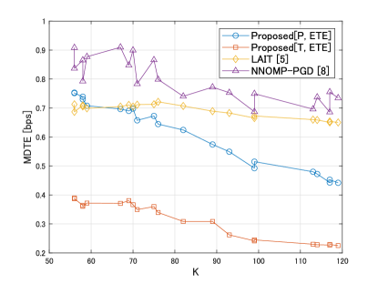
Figure 1: The graph of $\operatorname{MDTE}[\mathrm{bps}]$ across different sparsity on S&P500, 2012 - 2017. The vertical axis indicates $\operatorname{MDTE}[\mathrm{bps}]$ and the horizontal axis indicates the sparsity. To avoid parameter tuning on $\lambda$ (which controls sparsity in LAIT), we fixed the value of $\lambda$ per data point. Therefore, the exact sparsity of per training period differs. The sparsity of Proposed[P, ETE] ($K_{1}$) and NNOMP-PGD is adjusted to be the same as that of LAIT. As for Proposed[T, ETE], $K_{2}=K_{1}$. Parameter $K$ in the graph indicates the sparsity of the portfolio at $n=10$.

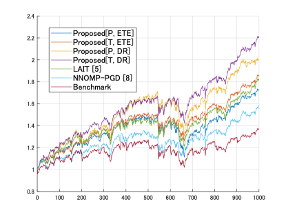
Figure 2: The graph of the investment simulation on S&P500, 2012 - 2017. The vertical axis indicates the normalized accumulated return and the horizontal axis indicates the sparsity of the portfolio ($K_{1},K_{2},K=56$). The graph indicates an investment simulation based on one of the data points of Fig. 1. The initial capital is $\$10000$.

4.2 Results

4.2.1 Tracking Performance

Our proposed method generally outperformed NNOMP-PGD and LAIT on the S&P500 dataset (Fig. 1). Furthermore, Proposed[P, ETE] delivered superior performance to NNOMP-PGD across all settings (Tables 1 and 2 (MDTE)). This supports our hypothesis that concurrent asset selection and capital allocation can be advantageous. Both strategies, Proposed[P, ETE] and NNOMP-PGD, are predicated on similar $\ell_{0}$-norm constraints and tracking error measures, with the primary distinction lying in the solving algorithm used. Note that LAIT is not included in Tables 1 and 2 due to the difficulties encountered in adjusting the sparsity to an exact value using LAIT.

Furthermore, comparing the tracking performance of portfolio-sparse (Proposed[P, ETE]) methods and turnover-sparse (Proposed[T, ETE]) methods, we can see that turnover-sparse methods always performed better. We believe this is because portfolios constructed using turnover-sparse methods are composed of more nonzero weights compared to those of portfolio-sparse methods. Because turnover-sparse methods only enforce sparseness of the turnover, the sparsity of the portfolio itself is not considered. Therefore, as the simulation progresses, the portfolio gradually becomes fuller. A fuller portfolio can replicate the target index with more nonzero weights, which should affect the tracking performance positively. Turnover-sparse methods with $K_{2}=K_{1}$ tracked the index more effectively than other $K_{2}$ values did, for the same reason, because larger $K_{2}$ values densify the portfolio faster than smaller $K_{2}$ values. Similarly, a larger $K_{1}$ performed better for portfolio-sparse methods, since portfolios constructed from larger $K_{1}$ values have more nonzero weights.

4.2.2 Return Accumulation

We were able to accumulate more returns compared to the benchmark index in all settings and NNOMP-PGD in most of the settings (Tables 1 and 2 (Ret.)). It is clear that sparse portfolios are much more efficient compared to benchmark (full) portfolios (Fig. 2). However, regarding comparisons between portfolio-sparse and turnover-sparse methods and the various tracking measures, we acquired varying results depending on dataset and period. First, when we applied the empirical tracking error (ETE) as the tracking measure, turnover-sparse methods (Proposed[T, ETE]) generally performed better than portfolio-sparse methods (Proposed[P, ETE]) with the exception of NASDAQ100 2015-2019. This seems intuitive since turnover-sparse methods sparsifise the turnover, which directly affects the transaction costs. In the worst case rebalancing scenario, portfolios constructed by portfolio-sparse methods sells all assets in possesion, and newly buys completely different assets. In this case the transaction cost would be $\$2K_{1}$ (assuming the minimum cost is dominant). In comparison, the worst case scenario for portfolios constructed by turnover-sparse methods is always $K_{2}$. However, examining how this behaviour differed in NASDAQ100 2015-2019, we expect some variance in the results depending on the dataset.

Next, when downside risk (DR) was applied, Proposed[P, DR] methods generally performed better than turnover-sparse methods (Proposed[T, DR]). Note that this was also inconsistent in NASDAQ100 2015-2019. Unfortunately, we do not have a rational explanation for this, but we speculate this caused by the vulnerable nature of a nonconvex formulation. We will further discuss this in Section 4.2.3. In addition to the above behaviour, DR applied methods performed moderately in comparison to ETE applied methods. We expected DR to accumulate more returns than ETE, but there are some results where ETE outperformed the DR counterpart. Although DR trades-off tracking accuracy for return, we can see from the results that the trade-off is not always beneficial.

4.2.3 Initialization

Because our formulation is not convex, the proposed algorithm does not guarantee convergence. Therefore, the method of initializing the parameter ${\mathbf{w}}$ may potentially impact the results. To explore the differences in initialization methods, we compared three methods. Init. A: ${\mathbf{w}}=\mathbf{0}$, the original initialization adopted in our algorithm (Algorithm 1). Init. B: initialize all elements of ${\mathbf{w}}$ to $1/N$. Init. C: initialize ${\mathbf{w}}$ by assigning $1/K_{1}$ to $K_{1}$ randomly selected elements of ${\mathbf{w}}$ when $S_{s}=S_{0}$, and initialize ${\mathbf{w}}$ as ${\mathbf{w}}={\mathbf{w}}_{0}$ when $S_{s}=S_{{\mathbf{w}}_{0}}$. The results are shown in Tables 3.

From how the results vary, it is evident that the initialization method affects the output. Since the results were inconsistent depending on dataset, we could not determine a superior initialization method. However, we would like to note that our method achieved better performance than NNOMP-PGD regardless of the initialization method in majority of the settings.

4.2.4 Practical Application

Based on the previous results and discussions, we would like to discuss the possibility of applying our methods to real-world investment situations. First, the data and variables used in our methods to construct the portfolios are available. Therefore, the main concern would be the choice of portfolio or turnover-sparsity and tracking error measures. Examining Tables 1 and 2, although we were unable to determine a method that consistently achieved best return accumulation performance across all datasets, the best performing method seems to be somewhat consistent within each of the datasets. We believe it is possible to use past data to determine a dataset-specific method to effectively track an index. In the same manner, parameters $K_{1}$ and $K_{2}$ can also be decided.

One of the pros of a sparse portfolio was that it can avoid illiquid assets. However, extensive application of turnover-sparse methods may result in dense or full portfolios, as discussed in Section 4.2.1. In real-life situations, we can simply reset the portfolio by applying the portfolio-sparse method every time unwanted (illiquid) assets start becoming included in the portfolio.

Although we did not explicitly discuss this in our paper, the length of $T_{\mathrm{train}}$ and $T_{\mathrm{test}}$ are also parameters. The two should be decided by simulating on past data, similarly to the other parameters.

4.2.5 Summary of the Experimental Results

Through extensive numerical experiments on S&P500 and NASDAQ100 datasets, we:

• Confirmed our hypothesis that simultaneous asset selection and capital allocation can be beneficial in terms of tracking accuracy.

• Presented the merits of turn-over sparsity in both index tracking and wealth accumulation.

• Explored various tracking error measures and their parameter to study their effects on performance.

• Discussed the effects different initialization methods have on the proposed algorithm.

• Discussed the possibility of applying our method to real-world investing.

5 Concluding Remarks

In this paper, we proposed a sparse index tracking method that addressed both asset selection and capital allocation simultaneously, enhancing tracking performance compared to the conventional method that handled these two aspects separately. Furthermore, the proposed formulation was generalized to allow the choice between 1) portfolio sparsity and turnover sparsity constraints, both enforced by an $\ell_{0}$-norm constraint, and 2) various tracking error measures aimed at enhancing return accumulation performance. Superior results were demonstrated through experiments on the S&P500 and NASDAQ100 index datasets, where we achieved state-of-the-art performance compared to the conventional method that incorporated an $\ell_{0}$-norm constraint. We also examined and discussed the impacts of different tracking measures and initializations.

References

- [1] B. Malkiel, “Passive investment strategies and efficient markets,” European Financial Management, vol. 9, pp. 1–10, 03 2003.
- [2] R. Fuller, B. Han, and Y. Tung, “Thinking about indices and “passive” versus active management,” Journal of Portfolio Management, vol. 36, pp. 35–47, 07 2010.
- [3] B. M. Barber and T. Odean, “Trading is hazardous to your wealth: The common stock investment performance of individual investors,” The journal of Finance, vol. 55, no. 2, pp. 773–806, 2000.
- [4] A. A. Gaivoronski, S. Krylov, and N. van der Wijst, “Optimal portfolio selection and dynamic benchmark tracking,” European Journal of Operational Research, vol. 163, no. 1, pp. 115–131, 2005, financial Modelling and Risk Management.
- [5] K. Benidis, Y. Feng, and D. P. Palomar, “Sparse portfolios for high-dimensional financial index tracking,” IEEE Transactions on Signal Processing, vol. 66, no. 1, pp. 155–170, 2018.
- [6] K. Benidis, Y. Feng, and D. P. Palomar, “Optimization methods for financial index tracking: From theory to practice,” Foundations and Trends® in Optimization, vol. 3, no. 3, pp. 171–279, 2018.
- [7] Y. Zheng, T. M. Hospedales, and Y. Yang, “Diversity and sparsity: A new perspective on index tracking,” in 2020 IEEE International Conference on Acoustics, Speech and Signal Processing (ICASSP), 2020, pp. 1768–1772.
- [8] X. P. Li, Z. Shi, C. Leung, and H. C. So, “Sparse index tracking with k-sparsity or -deviation constraint via -norm minimization,” IEEE Transactions on Neural Networks and Learning Systems, pp. 1–14, 2022.
- [9] M. Yaghoobi, D. Wu, and M. E. Davies, “Fast non-negative orthogonal matching pursuit,” IEEE Signal Processing Letters, vol. 22, no. 9, pp. 1229–1233, 2015.
- [10] T. T. Nguyen, J. Idier, C. Soussen, and E. Djermoune, “Non-negative orthogonal greedy algorithms,” IEEE Transactions on Signal Processing, vol. 67, no. 21, pp. 5643–5658, 2019.
- [11] L. Condat, “A primal–dual splitting method for convex optimization involving lipschitzian, proximable and linear composite terms,” Journal of Optimization Theory and Applications, vol. 158, 08 2013.
- [12] K. J. Oh, T. Y. Kim, and S. Min, “Using genetic algorithm to support portfolio optimization for index fund management,” Expert Systems with Applications, vol. 28, no. 2, pp. 371–379, 2005.
- [13] C. Dose and S. C., “Clustering of financial time series with application to index and enhanced index tracking portfolio,” Physica A: Statistical Mechanics and its Applications, vol. 355, no. 1, pp. 145–151, 2005, market Dynamics and Quantitative Economics.
- [14] D. Bianchi and A. Gargano, “High-dimensional index tracking with cointegrated assets using an hybrid genetic algorithm,” Capital Markets: Asset Pricing & Valuation eJournal, 03 2011.
- [15] C. A., “Optimal hedging using cointegration,” Philosophical Transactions of The Royal Society A: Mathematical, Physical and Engineering Sciences, vol. 357, pp. 2039–2058, 08 1999.
- [16] D. Maringer and O. Oyewumi, “Index tracking with constrained portfolios,” Int. Syst. in Accounting, Finance and Management, vol. 15, pp. 57–71, 06 2007.
- [17] J. Beasley, N. Meade, and T.-J. Chang, “An evolutionary heuristic for the index tracking problem,” European Journal of Operational Research, vol. 148, no. 3, pp. 621–643, 2003.
- [18] R. Jansen and R. Dijk, “Optimal benchmark tracking with small portfolios,” Journal of Portfolio Management, vol. 28, pp. 33–39, 12 2002.
- [19] J.-J. Moreau, “Dual convex functions and proximal points in a hilbert space,” CRAS, Paris, vol. 255, pp. 2897–2899, 1962.
- [20] B. C. Vu, “A splitting algorithm for dual monotone inclusions involving cocoercive operators,” Advances in Computational Mathematics, vol. 38, no. 3, pp. 667–681, 2013.
- [21] A. Chambolle and T. Pock, “A first-order primal-dual algorithm for convex problems with applications to imaging,” Journal of mathematical imaging and vision, vol. 40, no. 1, pp. 120–145, 2011.
- [22] H. H. Bauschke and P. L. Combettes, Convex Analysis and Monotone Operator Theory in Hilbert Spaces, 2nd ed. 2017 Edition. Springer, 2017.
- [23] L. Condat, “A generic proximal algorithm for convex optimization—application to total variation minimization,” IEEE Signal Processing Letters, vol. 21, no. 8, pp. 985–989, 2014.
- [24] S. Ono and I. Yamada, “Hierarchical convex optimization with primal-dual splitting,” IEEE Transactions on Signal Processing, vol. 63, no. 2, pp. 373–388, 2014.
- [25] S. Ono, “Primal-dual plug-and-play image restoration,” IEEE Signal Processing Letters, vol. 24, no. 8, pp. 1108–1112, 2017.
- [26] J. Boulanger, N. Pustelnik, L. Condat, L. Sengmanivong, and T. Piolot, “Nonsmooth convex optimization for structured illumination microscopy image reconstruction,” Inverse Problems, vol. 34, no. 9, p. 095004, 2018.
- [27] S. Kyochi, S. Ono, and I. W. Selesnick, “Epigraphical relaxation for minimizing layered mixed norms,” IEEE Transactions on Signal Processing, vol. 69, pp. 2923–2938, 2021.
- [28] S. Takemoto, K. Naganuma, and S. Ono, “Graph spatio-spectral total variation model for hyperspectral image denoising,” IEEE Geoscience and Remote Sensing Letters, vol. 19, pp. 1–5, 2022.
- [29] K. Naganuma and S. Ono, “A general destriping framework for remote sensing images using flatness constraint,” IEEE Transactions on Geoscience and Remote Sensing, vol. 60, pp. 1–16, 2022.
- [30] E. Yamagata and S. Ono, “Robust time-varying graph signal recovery for dynamic physical sensor network data,” arXiv:2202.06432, 2023.
- [31] N. Komodakis and J.-C. Pesquet, “Playing with duality: An overview of recent primal-dual approaches for solving large-scale optimization problems,” IEEE Signal Processing Magazine, vol. 32, no. 6, pp. 31–54, 2015.
- [32] M. Hong, Z. Luo, and M. Razaviyayn, “Convergence analysis of alternating direction method of multipliers for a family of nonconvex problems,” in 2015 IEEE International Conference on Acoustics, Speech and Signal Processing (ICASSP), 2015, pp. 3836–3840.
- [33] G. Li and T. Pong, “Global convergence of splitting methods for nonconvex composite optimization,” SIAM Journal on Optimization, vol. 25, pp. 2434–2460, 09 2015.
- [34] S. Ono, “ gradient projection,” IEEE Transactions on Image Processing, vol. 26, no. 4, p. 1554–1564, Apr. 2017.
- [35] L. Condat and A. Hirabayashi, “Cadzow denoising upgraded: A new projection method for the recovery of dirac pulses from noisy linear measurements,” Sampling Theory in Signal and Image Processing, vol. 14, no. 1, pp. 17–47, 2015.
- [36] A. Takeda, M. Niranjan, J. Gotoh, and Y. Kawahara, “Simultaneous pursuit of out-of-sample performance and sparsity in index tracking portfolios,” Computational Management Science, vol. 10, no. 1, pp. 21–49, 2013.