A Geometric Framework for Neural Feature Learning

Abstract

We present a novel framework for learning system design based on neural feature extractors. First, we introduce the feature geometry, which unifies statistical dependence and features in the same function space with geometric structures. By applying the feature geometry, we formulate each learning problem as solving the optimal feature approximation of the dependence component specified by the learning setting. We propose a nesting technique for designing learning algorithms to learn the optimal features from data samples, which can be applied to off-the-shelf network architectures and optimizers. To demonstrate the applications of the nesting technique, we further discuss multivariate learning problems, including conditioned inference and multimodal learning, where we present the optimal features and reveal their connections to classical approaches.

Keywords: Feature geometry, information processing, neural feature learning, nesting technique, multivariate dependence decomposition

1 Introduction

Learning useful feature representations from data observations is a fundamental task in machine learning. Early developments of such algorithms focused on learning optimal linear features, e.g., linear regression, PCA (Principal Component Analysis) (Pearson, 1901), CCA (Canonical Correlation Analysis) (Hotelling, 1936), and LDA (Linear Discriminant Analysis) (Fisher, 1936). The resulting algorithms admit straightforward implementations, with well-established connections between learned features and statistical behaviors of data samples. However, practical learning applications often involve data with complex structures which linear features fail to capture. To address such problems, practitioners employ more complicated feature designs and build inference models based on these features, e.g., kernel methods (Cortes and Vapnik, 1995; Hofmann et al., 2008) and deep neural networks (LeCun et al., 2015). The feature representations serve as the information carrier, capturing useful information from data for subsequent processing. An illustration of such feature-centric learning systems is shown in Figure 1, which consists of two parts:

1. A learning module which generates a collection of features from the data. Data can take different forms, for example, input-output pairs or some tuples. The features can be either specified implicitly, e.g., by a kernel function in kernel methods, or explicitly parameterized as feature extractors, e.g., artificial neural networks. The features are learned via a training process, e.g., optimizing a training objective defined on the features.

2. An assembling module which uses learned features to build an inference model or a collection of inference models. The inference models are used to provide information about data. For example, when the data take the form of input-output pairs, a typical inference model provides prediction or estimation of output variables based on the input variables. The assembling module determines the relation between features and resulting models, which can also be specified implicitly, e.g., in kernel methods.

Figure 1: Schematic diagram of a general feature-centric learning system

Learning systems are commonly designed with a predetermined assembling module, which allows the whole system to be learned in an end-to-end manner. One representative example of such designs is deep neural networks. On one hand, this end-to-end characteristic makes it possible to exploit large-scale and often over-parametrized neural feature extractors (LeCun et al., 2015; Krizhevsky et al., 2017; He et al., 2016; Vaswani et al., 2017), which can effectively capture hidden structures in data. On the other hand, the choices of assembling modules and learning objectives are often empirically designed, with design heuristics varying a lot across different tasks. Such heuristic choices make the learned feature extractors hard to interpret and adapt, often viewed as black boxes. In addition, the empirical designs are typically inefficient, especially for multivariate learning problems, e.g., multimodal learning (Ngiam et al., 2011), where there can exist many potentially useful assembling modules and learning objectives to consider.

To address this issue and obtain more principled designs, recent developments have adopted statistical and information-theoretical tools in designing training objectives. The design goal is to guarantee that learned features are informative, i.e., carry useful information for the inference tasks. To this end, a common practice is to incorporate information measures in learning objectives, such as mutual information (Tishby et al., 2000; Tishby and Zaslavsky, 2015) and rate distortion function (Chan et al., 2022). However, information measures might not effectively characterize the usefulness of features for learning tasks, due to the essentially different information processing natures. For example, originally introduced in characterizing the optimal rate of a communication system (Shannon, 1948), the mutual information is invariant to bijective transformations on variables—as the amount of information to communicate does not change after such transformations. As a consequence, when we consider the mutual information between feature representations and the input/output variables (Tishby and Zaslavsky, 2015), features up to such bijective transformations, e.g., sigmoid or exponential mappings, are all equivalent and give the same mutual information. This is in contrast to their often highly distinct performances on learning tasks. Due to this intrinsic discrepancy, it is often impractical to learn features based solely on the information measures. As a compromise, the information measures are often applied to analyze features learned from other objectives (Tishby and Zaslavsky, 2015), or used as regularization terms in the training objective to facilitate learning (Belghazi et al., 2018), where the learned features generally depend on case-by-case design choices.

In this work, we aim to establish a framework for learning features that capture the statistical nature of data, and can be assembled to build different inference models without retraining. In particular, the features are learned to approximate and represent the statistical dependence of data, instead of solving specific inference tasks. To this end, we introduce a geometry on function spaces, coined feature geometry, which we apply to connect statistical dependence with features. This connection allows us to represent statistical dependence by corresponding operations in feature spaces. Specifically, the features are learned by approximating the statistical dependence, and the approximation error measures the amount of information captured by features. The resulting features capture the statistical dependence and thus are useful for general inference tasks.

Our main contributions of this work are as follows.

• We establish a framework for designing learning systems that separate feature learning and feature usages, where the learned features can be assembled to build different inference models without retraining. In particular, we introduce the feature geometry, which converts feature learning problems to geometric operations in function space. The resulting optimal features capture the statistical dependence of data and can be adapted to different inference tasks.

• We propose a nesting technique for decomposing statistical dependence and learning the associated feature representations. The nesting technique provides a systematic approach to construct training objectives and develop learning algorithms, where we can learn optimal features by employing the state-of-the-art deep learning practices, e.g., network architecture and optimizer designs.

• We present the applications of this unified framework in multivariate learning problems, where we design feature learning algorithms to decompose and represent the corresponding multivariate dependence. As case studies, we consider the learning problem for conditioned inference and multimodal learning with missing modalities. We investigate the optimal features and demonstrate their relations to classical learning problems, such as maximum likelihood estimation and the maximum entropy principle (Jaynes, 1957a, b).

The rest of the paper is organized as follows. In Section 2, we introduce the feature geometry, including operations on feature spaces and functional representations of statistical dependence. In Section 3, we present the learning system design in a bivariate learning setting, where we demonstrate the feature learning algorithm and the design of assembling modules. In Section 4, we introduce the nesting technique, as a systematic approach to learning algorithm design in multivariate learning problems. We then demonstrate the applications of the nesting technique, where we study a conditioned inference problem in Section 5, and a multimodal learning problem in Section 6. Then, we present our experimental verification for the proposed learning algorithms in Section 7, where we compare the learned features with the theoretical solutions. Finally, we summarize related works in Section 8 and provide some concluding remarks in Section 9.

2 Notations and Preliminaries

For a random variable $Z$, we use $\mathcal{Z}$ to denote the corresponding alphabet, and use $z$ to denote a specific value in $\mathcal{Z}$. We use $P_{Z}$ to denote the probability distribution of $Z$.

For the sake of simplicity, we present our development with finite alphabets and associated discrete random variables. The corresponding results can be readily extended to general alphabets under certain regularity conditions, which we discuss in Appendix A.1 for completeness.

2.1 Feature Geometry

2.1.1 Vector Space

Given an inner product space with inner product $\langle\cdot,\cdot\rangle$ and its induced norm $\|\cdot\|$, we can define the projection and orthogonal complement as follows.

Definition 1

Give a subspace $\mathcal{W}$ of $\mathcal{V}$, we denote the projection of a vector $v\in\mathcal{V}$ onto $\mathcal{W}$ by

$$\Pi\left(v;{\mathcal{W}}\right)\triangleq\operatorname*{arg\,min}_{w\in\mathcal{W}}\left\|v-w\right\|^{2}.$$ (1)

In addition, we use $\mathcal{V}\mathbin{\boxminus}\mathcal{W}$ to denote the orthogonal complement of $\mathcal{W}$ in $\mathcal{V}$, viz., $\mathcal{V}\mathbin{\boxminus}\mathcal{W}\triangleq\{v\in\mathcal{V}\colon\langle v,w\rangle=0\text{ for all }w\in\mathcal{W}\}$.

We use “$\mathbin{\boxplus}$” to denote the direct sum of orthogonal subspaces, i.e., $\mathcal{V}=\mathcal{V}_{1}\mathbin{\boxplus}\mathcal{V}_{2}$ indicates that $\mathcal{V}=\mathcal{V}_{1}+\mathcal{V}_{2}$ and $\mathcal{V}_{1}\perp\mathcal{V}_{2}$. Then we have the following facts.

Fact 1

If $\mathcal{V}=\mathcal{V}_{1}\mathbin{\boxplus}\mathcal{V}_{2}$, then $\mathcal{V}_{2}=\mathcal{V}\mathbin{\boxminus}\mathcal{V}_{1}$. In addition, if $\mathcal{W}$ is a subspace of $\mathcal{V}$, then $\mathcal{V}=\mathcal{W}\mathbin{\boxplus}(\mathcal{V}\mathbin{\boxminus}\mathcal{W})$.

Fact 2 (Orthogonality Principle)

Given $v\in\mathcal{V}$ and a subspace $\mathcal{W}$ of $\mathcal{V}$, then $w=\Pi\left(v;{\mathcal{W}}\right)$ if and only if $w\in\mathcal{W}$ and $v-w\in\mathcal{V}\mathbin{\boxminus}\mathcal{W}$. In addition, we have $v=\Pi\left(v;{\mathcal{W}}\right)+\Pi\left(v;{\mathcal{V}\mathbin{\boxminus}\mathcal{W}}\right)$.

2.1.2 Feature Space

Given an alphabet $\mathcal{Z}$, we use $\mathcal{P}^{\mathcal{Z}}$ to denote the collection of probability distributions supported on $\mathcal{Z}$, and use $\operatorname{relint}(\mathcal{P}^{\mathcal{Z}})$ to denote the relative interior of $\mathcal{P}^{\mathcal{Z}}$, i.e., the collection of distributions $P\in\mathcal{P}^{\mathcal{Z}}$ with $P(z)>0$ for all $z\in\mathcal{Z}$.

We use $\mathcal{F}_{\mathcal{Z}}\triangleq\{\mathcal{Z}\to\mathbb{R}\}$ to denote the collection of features (functions) on given $\mathcal{Z}$. Specifically, we use $\mathtt{1}_{\mathcal{Z}}\in\mathcal{F}_{\mathcal{Z}}$ to denote the constant feature that takes value 1, i.e., $\mathtt{1}_{\mathcal{Z}}(z)\equiv 1$ for all $z\in\mathcal{Z}$. We define the inner product on $\mathcal{F}_{\mathcal{Z}}$ as $\langle f_{1},f_{2}\rangle\triangleq{\mathbb{E}}_{R}\left[f_{1}(Z)f_{2}(Z)\right]$, where $R\in\operatorname{relint}(\mathcal{P}^{\mathcal{Z}})$ is referred to as the metric distribution. This defines the geometric operations on $\mathcal{F}_{\mathcal{Z}}$, e.g., norm and projection. Specifically, we have the induced norm $\|f\|\triangleq\sqrt{\langle f,f\rangle}$, and the projection of $f\in\mathcal{F}_{\mathcal{Z}}$ onto a subspace $\mathcal{G}_{\mathcal{Z}}$ of $\mathcal{F}_{\mathcal{Z}}$, i.e., $\Pi\left(f;{\mathcal{G}_{\mathcal{Z}}}\right)$, is defined according to Definition 1. We also use $\tilde{\mathcal{F}}_{\mathcal{Z}}\triangleq\{f\in\mathcal{F}_{\mathcal{Z}}\colon{\mathbb{E}}_{R}\left[f(Z)\right]=0\}$ to denote the collection of zero-mean features on $\mathcal{Z}$, which corresponds to the orthogonal complement of constant features, i.e., $\tilde{\mathcal{F}}_{\mathcal{Z}}=\mathcal{F}_{\mathcal{Z}}\mathbin{\boxminus}\operatorname{span}\{\mathtt{1}_{\mathcal{Z}}\}$.

For each $k\geq 1$, we use $\mathcal{F}_{\mathcal{Z}}^{\,k}\triangleq\left(\mathcal{F}_{\mathcal{Z}}\right)^{k}=\{\mathcal{Z}\to\mathbb{R}^{k}\}$ to denote the collection of $k$-dimensional features. For $f\in\mathcal{F}_{\mathcal{Z}}^{\,k}$, we use $\operatorname{span}\{f\}\subset\mathcal{F}_{\mathcal{Z}}$ to denote the subspace of $\mathcal{F}_{\mathcal{Z}}$ spanned by all dimensions of $f$, i.e., $\operatorname{span}\{f\}=\operatorname{span}\{f_{1},\dots,f_{k}\}$, and use $\Pi\left(f;{\mathcal{G}_{\mathcal{Z}}}\right)$ to denote the corresponding projection on each dimension, i.e., $\Pi\left(f;{\mathcal{G}_{\mathcal{Z}}}\right)=[\Pi\left(f_{1};{\mathcal{G}_{\mathcal{Z}}}\right),\dots,\Pi\left(f_{k};{\mathcal{G}_{\mathcal{Z}}}\right)]^{\mathrm{T}}\in\mathcal{G}_{\mathcal{Z}}^{\,k}\triangleq(\mathcal{G}_{\mathcal{Z}})^{k}$. For $f_{1}\in\mathcal{F}_{\mathcal{Z}}^{\,k_{1}},f_{2}\in\mathcal{F}_{\mathcal{Z}}^{\,k_{2}}$, we denote $\Lambda_{f_{1},f_{2}}\triangleq{\mathbb{E}}_{R}\left[f_{1}(Z)f_{2}^{\mathrm{T}}(Z)\right]$. Specifically, we define $\Lambda_{f}\triangleq\Lambda_{f,f}={\mathbb{E}}_{R}\left[f(Z)f^{\mathrm{T}}(Z)\right]$ for feature $f\in\mathcal{F}_{\mathcal{Z}}^{\,k}$. We also use $[k]$ to denote the set $\{i\in\mathbb{Z}\colon 1\leq i\leq k\}$ with ascending order, and define $f_{[k]}\in\mathcal{F}_{\mathcal{Z}}^{\,k}$ as $f_{[k]}\colon z\mapsto(f_{1}(z),\dots,f_{{k}}(z))^{\mathrm{T}}$ for given $f_{1},\dots,f_{k}\in\mathcal{F}_{\mathcal{Z}}$.

2.1.3 Neural Feature Extractors

Our development will focus on neural feature extractors, i.e., features represented by neural networks. To begin, we consider a neural network of a given architecture with $m$ trainable parameters and $k$-dimensional outputs. Let $\mathcal{Z}$ denote the domain of input data $Z$, and denote the trainable parameters by $\underline{\theta}\in\mathbb{R}^{m}$. Then, for each $\underline{\theta}\in\mathbb{R}^{m}$, we can denote the associated neural feature as $f^{(\underline{\theta})}\in\mathcal{F}_{\mathcal{Z}}^{\,k}$.

For the sake of simplicity, our discussions focus on the ideal case where the neural network has sufficient expressive power, i.e., each feature in $\mathcal{F}_{\mathcal{Z}}^{\,k}$ can be well-approximated by a large $m$ and some $\theta\in\mathbb{R}^{m}$. Under this idealized assumption, optimizing over network parameters $\underline{\theta}$ is equivalent to finding the optimal $f\in\mathcal{F}_{\mathcal{Z}}^{\,k}$. Therefore, we will omit the network parameter $\theta$ and use $f$ to denote such neural feature extractor, which we represented as a trapezoid block, as shown in Figure 2a.

(a) Feature Extractor

(b) Linear Layer

(c) Feature Subspace

Figure 2: Schematic representations of neural feature extractors. LABEL:sub@fig:nfe:f: a general feature extractor $f\in\mathcal{F}_{\mathcal{Z}}^{\,k}$; LABEL:sub@fig:nfe:wb: a linear layer with weight matrix $W$ and bias $\underline{b}$; LABEL:sub@fig:nfe:sspc: the composition of feature extractor blocks, where each dimension of the output lies in the feature subspace $\operatorname{span}\{\phi\}$.

Linear layer is an important building block in neural feature extractors, which performs an affine transformation on the input, as shown in Figure 2b. In particular, a linear layer with input dimension $d$ and output dimension $k$ is specified by a weight matrix $W\in\mathbb{R}^{k\times d}$ and bias vector $\underline{b}\in\mathbb{R}^{k}$, which outputs $W\underline{v}+\underline{b}$ for an input $\underline{v}\in\mathbb{R}^{d}$. We can use linear layers to construct feature subspaces, as shown in Figure 2c, where we have considered a given $d$-dimensional feature $\phi=(\phi_{1},\dots,\phi_{d})^{\mathrm{T}}\in\mathcal{F}_{\mathcal{X}}^{\,d}$ and a linear layer without the bias term. Then, the collection of output features by varying weight matrix $W$ is $\{W\phi\colon W\in\mathbb{R}^{k\times d}\}=\operatorname{span}^{k}\{\phi\}$. Note that since the generated features are restricted to a subspace, the cascaded feature extractor has restricted expressive power, which can generally affect the feature learning. We will discuss such effects in our later developments (cf. Section 3.3).

2.1.4 Joint Functions

Given alphabets $\mathcal{X},\mathcal{Y}$ and a metric distribution $R_{X,Y}\in\operatorname{relint}(\mathcal{P}^{\mathcal{X}\times\mathcal{Y}})$, $\mathcal{F}_{\mathcal{X}\times\mathcal{Y}}$ is composed of all joint functions of $x$ and $y$. In particular, for given $f\in\mathcal{F}_{\mathcal{X}}$, $g\in\mathcal{F}_{\mathcal{Y}}$, we use $f\otimes g$ to denote their product $\left((x,y)\mapsto f(x)\cdot g(y)\right)\in\mathcal{F}_{\mathcal{X}\times\mathcal{Y}}$, and refer to such functions as product functions. For each product function $\gamma\in\mathcal{F}_{\mathcal{X}\times\mathcal{Y}}$, we can find $\sigma=\|\gamma\|\geq 0$, and $f\in\mathcal{F}_{\mathcal{X}},g\in\mathcal{F}_{\mathcal{Y}}$ with $\|f\|=\|g\|=1$, such that

$$\gamma=\sigma\cdot(f\otimes g).$$ (2)

We refer to (2) as the standard form of product functions.

In addition, for given $f=(f_{1},\dots,f_{k})^{\mathrm{T}}\in\mathcal{F}_{\mathcal{X}}^{\,k}$ and $g=(g_{1},\dots,g_{k})^{\mathrm{T}}\in\mathcal{F}_{\mathcal{Y}}^{\,k}$, we denote $f\otimes g\triangleq\sum_{i=1}^{k}f_{i}\otimes g_{i}$. For two subspaces $\mathcal{G}_{\mathcal{X}}$ and $\mathcal{G}_{\mathcal{Y}}$ of $\mathcal{F}_{\mathcal{X}}$ and $\mathcal{F}_{\mathcal{Y}}$, respectively, we denote the tensor product of $\mathcal{G}_{\mathcal{X}}$ and $\mathcal{G}_{\mathcal{Y}}$ as $\mathcal{G}_{\mathcal{X}}\otimes\mathcal{G}_{\mathcal{Y}}\triangleq\operatorname{span}\{f\otimes g\colon f\in\mathcal{G}_{\mathcal{X}},g\in\mathcal{G}_{\mathcal{Y}}\}$.

Note that by extending each $f=(x\mapsto f(x))\in\mathcal{F}_{\mathcal{X}}$ to $\left((x,y)\mapsto f(x)\right)\in\mathcal{F}_{\mathcal{X}\times\mathcal{Y}}$, $\mathcal{F}_{\mathcal{X}}$ becomes a subspace of $\mathcal{F}_{\mathcal{X}\times\mathcal{Y}}$, with the metric distribution being the marginal distribution $R_{X}$ of $R_{X,Y}$. We then denote the orthogonal complement of $\mathcal{F}_{\mathcal{X}}$ in $\mathcal{F}_{\mathcal{X}\times\mathcal{Y}}$ as

$$\mathcal{F}_{\mathcal{Y}|\mathcal{X}}\triangleq\mathcal{F}_{\mathcal{X}\times\mathcal{Y}}\mathbin{\boxminus}\mathcal{F}_{\mathcal{X}}.$$ (3)

We establish a correspondence between the distribution space $\mathcal{P}^{\mathcal{Z}}$ and the feature space $\mathcal{F}_{\mathcal{Z}}$ by the density ratio function.

Definition 2

Given a metric distribution $R\in\operatorname{relint}(\mathcal{P}^{\mathcal{Z}})$, for each $P\in\mathcal{P}^{\mathcal{Z}}$, we define the (centered) density ratio function $\tilde{\ell}_{P;R}\in\mathcal{F}_{\mathcal{Z}}$ as

$$\tilde{\ell}_{P;R}(z)\triangleq\frac{P(z)-R(z)}{R(z)},\quad\text{for all }z\in\mathcal{Z}.$$

It is easy to verify that $\tilde{\ell}_{P;R}$ has mean zero , i.e., $\tilde{\ell}_{P;R}\in\tilde{\mathcal{F}}_{\mathcal{Z}}$. We will simply refer to $\tilde{\ell}_{P;R}$ as the density ratio or likelihood ratio and use $\tilde{\ell}_{P}$ to denote $\tilde{\ell}_{P;R}$ when there is no ambiguity about the metric distribution $R$.

In particular, given random variables $X$ and $Y$ with the joint distribution $P_{X,Y}$, we denote the density ratio $\tilde{\ell}_{P_{X,Y};P_{X}P_{Y}}$ by $\mathfrak{i}_{X;Y}$, i.e.,

$$\mathfrak{i}_{X;Y}(x,y)=\frac{P_{X,Y}(x,y)-P_{X}(x)P_{Y}(y)}{P_{X}(x)P_{Y}(y)},\quad\text{for all $x\in\mathcal{X},y\in\mathcal{Y}$.}$$ (4)

We refer to $\mathfrak{i}_{X;Y}$ as the canonical dependence kernel (CDK) function, which connects the $(X;Y)$ dependnece with $\mathcal{F}_{\mathcal{X}\times\mathcal{Y}}$.

With the feature geometry, we can associate geometric operations with corresponding operations on features, which we summarize as follows.

Property 1

Consider the feature geometry on $\mathcal{F}_{\mathcal{X}\times\mathcal{Y}}$ defined by the metric distribution $R_{X,Y}=P_{X}P_{Y}$. Then, we have $\langle f_{1}\otimes g_{1},f_{2}\otimes g_{2}\rangle={\mathbb{E}}_{P_{X}}\left[f_{1}(X)f_{2}(X)\right]\cdot{\mathbb{E}}_{P_{Y}}\left[g_{1}(Y)g_{2}(Y)\right]$ for given $f_{1},f_{2}\in\mathcal{F}_{\mathcal{X}},g_{1},g_{2}\in\mathcal{F}_{\mathcal{Y}}$. In addition, For any $k\geq 1$ and $f\in\mathcal{F}_{\mathcal{X}}^{\,k},g\in\mathcal{F}_{\mathcal{Y}}^{\,k}$, we have

$$\Pi\left(f;{\operatorname{span}\{\mathtt{1}_{\mathcal{X}}\}}\right)={\mathbb{E}}_{P_{X}}\left[f(X)\right],\quad\Pi\left(f;{\tilde{\mathcal{F}}_{\mathcal{X}}}\right)=f-{\mathbb{E}}_{P_{X}}\left[f(X)\right],$$ (5)

$$\langle\mathfrak{i}_{X;Y},f\otimes g\rangle={\mathbb{E}}_{P_{X,Y}}\left[f^{\mathrm{T}}(X)g(Y)\right]-\left({\mathbb{E}}_{P_{X}}\left[f(X)\right]\right)^{\mathrm{T}}{\mathbb{E}}_{P_{Y}}\left[g(Y)\right],$$ (6)

$$\|f\otimes g\|^{2}=\operatorname{tr}(\Lambda_{f}\Lambda_{g}),$$ (7)

where $\Lambda_{f}={\mathbb{E}}_{P_{X}}\left[f(X)f^{\mathrm{T}}(X)\right],\Lambda_{g}={\mathbb{E}}_{P_{Y}}\left[g(Y)g^{\mathrm{T}}(Y)\right]$.

2.1.5 Feature Geometry on Data Samples

In practice, the variables of interest typically have unknown and complicated probability distributions, with only data samples available for learning. We can similarly define the feature geometry on data samples by exploiting the corresponding empirical distributions.

To begin, given a dataset consisting of $n$ samples of $Z$, denoted as $\{z_{i}\}_{i=1}^{n}$, we denote the corresponding empirical distribution $\hat{P}_{Z}\in\mathcal{P}^{\mathcal{Z}}$ as

$$\hat{P}_{Z}(z)\triangleq\frac{1}{n}\sum_{i=1}^{n}\mathbbb{1}_{\{z_{i}=z\}},\quad\text{for all }z\in\mathcal{Z},$$ (8)

where $\mathbbb{1}_{\{\cdot\}}$ denotes the indicator function. Then, for any function $f$ of $Z$, we have ${\mathbb{E}}_{\hat{P}_{Z}}\left[f(Z)\right]=\sum_{z\in\mathcal{Z}}\hat{P}_{Z}(z)\cdot f(z)=\frac{1}{n}\sum_{i=1}^{n}f(z_{i})$, which is the empirical average of $f$ over the dataset.

Specifically, given $n$ sample pairs $\mathscr{D}=\{(x_{i},y_{i})\}_{i=1}^{n}$ of $(X,Y)$, the corresponding joint empirical distribution $\hat{P}_{X,Y}\in\mathcal{P}^{\mathcal{X}\times\mathcal{Y}}$ is given by

$$\hat{P}_{X,Y}(x,y)=\frac{1}{n}\sum_{i=1}^{n}\mathbbb{1}_{\{x_{i}=x,y_{i}=y\}},\quad\text{for all }x\in\mathcal{X},y\in\mathcal{Y}.$$ (9)

It is easily verified that the marginal distributions of $\hat{P}_{X,Y}$ are the empirical distributions $\hat{P}_{X}$ of $\{x_{i}\}_{i=1}^{n}$ and $\hat{P}_{Y}$ of $\{y_{i}\}_{i=1}^{n}$. Therefore, we can express the CDK function associated with the empirical distribution $\hat{P}_{X,Y}$ as [cf. (4)]

$$\hat{\mathfrak{i}}_{X;Y}(x,y)=\frac{\hat{P}_{X,Y}(x,y)-\hat{P}_{X}(x)\hat{P}_{Y}(y)}{\hat{P}_{X}(x)\hat{P}_{Y}(y)},\quad\text{for all $x\in\mathcal{X},y\in\mathcal{Y}$}.$$ (10)

As a result, given the dataset $\mathscr{D}$, we can define the associated feature geometry on $\mathcal{F}_{\mathcal{X}\times\mathcal{Y}}$ by using the metric distribution $R_{X,Y}=\hat{P}_{X}\hat{P}_{Y}$. From Property 1, we can evaluate the induced geometric quantities over data samples in $\mathscr{D}$, by replacing the distributions by the corresponding empirical distributions, and applying the empirical CDK function $\hat{\mathfrak{i}}_{X;Y}$ in (6).

Such characteristic allows us to discuss theoretical properties and algorithmic implementations in a unified notation. In our later developments, we will state both theoretical results and algorithms designs using the same notation of distribution, say, $P_{X,Y}$. This $P_{X,Y}$ corresponds to the underlying distribution in theoretical analyses, and represents the corresponding empirical distribution in algorithm implementations.

Remark 3

Note that for finite $\mathcal{Z}$, $\mathcal{F}_{\mathcal{Z}}$ is a space with a finite dimension $|\mathcal{Z}|$. Therefore, we can choose a basis of $\mathcal{F}_{\mathcal{Z}}$ and represent each feature as corresponding coefficient vectors in Euclidean space $\mathbb{R}^{|\mathcal{Z}|}$. Similarly, we can represent operators on function spaces as matrices. Such conventions have been introduced and adopted in previous works, e.g., (Huang et al., 2019; Xu et al., 2022), which we summarize in Appendix A.2 for completeness and comparisons.

2.2 Modal Decomposition

We then investigate a representation of joint functions in $\mathcal{F}_{\mathcal{X}\times\mathcal{Y}}$ by using features in $\mathcal{F}_{\mathcal{X}}$ and $\mathcal{F}_{\mathcal{Y}}$. This representation will be our basic tool to connect statistical dependence with feature spaces. Throughout this section, we set the metric distribution of $\mathcal{F}_{\mathcal{X}\times\mathcal{Y}}$ to the product form, i.e., $R_{X,Y}=R_{X}R_{Y}$. This induced metric distributions on $\mathcal{F}_{\mathcal{X}}$ and $\mathcal{F}_{\mathcal{Y}}$ are $R_{X}$ and $R_{Y}$, respectively.

2.2.1 Definitions and Properties

We use the operator $\operatorname{\zeta}$ on $\mathcal{F}_{\mathcal{X}\times\mathcal{Y}}$ to denote the optimal rank-1 approximation, i.e.,

$$\operatorname{\zeta}(\gamma)\triangleq\operatorname*{arg\,min}_{\begin{subarray}{c}\gamma^{\prime}\colon\gamma^{\prime}=f\otimes g\\ f\in\mathcal{F}_{\mathcal{X}},g\in\mathcal{F}_{\mathcal{Y}}\end{subarray}}\|\gamma-\gamma^{\prime}\|,\quad\text{for all $\gamma\in\mathcal{F}_{\mathcal{X}\times\mathcal{Y}}$}.$$ (11)

In addition, for all $k\geq 1$, we define the operator $\operatorname{\zeta}_{k}$ as $\operatorname{\zeta}_{1}\triangleq\operatorname{\zeta}$ and

$$\qquad\operatorname{\zeta}_{k}(\gamma)\triangleq\operatorname{\zeta}\left(\gamma-\sum_{i=1}^{k-1}\operatorname{\zeta}_{i}(\gamma)\right),$$ (12)

which we refer to as the $k$-th mode of $\gamma$. Then, we use

$$\operatorname{\zeta}_{\leq k}(\gamma)\triangleq\sum_{i=1}^{k}\operatorname{\zeta}_{i}(\gamma)\qquad\text{and}\qquad r_{k}(\gamma)\triangleq\gamma-\operatorname{\zeta}_{\leq k}(\gamma)$$ (13)

to denote the superposition of the top $k$ modes and the corresponding remainder, respectively.

Remark 4

If the minimization problem (11) has multiple solutions, the corresponding $\operatorname{\zeta}(\gamma)$ (and $\operatorname{\zeta}_{k}(\gamma)$) might not be unique. In this case, $\operatorname{\zeta}_{1}(\gamma),\dots\operatorname{\zeta}_{k}(\gamma)$ represent one of such solutions obtained from the sequential rank-1 approximations.

For each $\gamma\in\mathcal{F}_{\mathcal{X}\times\mathcal{Y}}$, we define the rank of $\gamma$ as $\operatorname{rank}(\gamma)\triangleq\inf\{k\geq 0\colon\|r_{k}(\gamma)\|=0\}$. Suppose $K\triangleq\operatorname{rank}(\gamma)$, then from the definition (13), we have $\gamma=\operatorname{\zeta}_{\leq K}(\gamma)+r_{K}(\gamma)=\operatorname{\zeta}_{\leq K}(\gamma)$, i.e.,

$$\gamma=\sum_{i=1}^{K}\operatorname{\zeta}_{i}(\gamma).$$ (14)

For each $i\in[K]$, let us denote the standard form [cf. (2)] of $\operatorname{\zeta}_{i}(\gamma)$ by $\operatorname{\zeta}_{i}(\gamma)=\sigma_{i}\left(f_{i}^{*}\otimes g_{i}^{*}\right)$. Therefore, from (14) we obtain

$$\gamma(x,y)=\sum_{i=1}^{K}\sigma_{i}\cdot f_{i}^{*}(x)\cdot g_{i}^{*}(y),\quad\text{for all $x\in\mathcal{X}$, $y\in\mathcal{Y}$},$$ (15)

where $\|f_{i}^{*}\|=\|g_{i}^{*}\|=1$ and $\sigma_{i}=\|\operatorname{\zeta}_{i}(\gamma)\|$. We refer to (15) as the modal decomposition of $\gamma$, which is a special case of Schmidt decomposition (Schmidt, 1907; Ekert and Knight, 1995), or singular value decomposition (SVD) in function space. We list several useful characterizations as follows.

Fact 3

Let $K\triangleq\operatorname{rank}(\gamma)$, then $\sigma_{1}\geq\sigma_{2}\geq\dots\geq\sigma_{K}>0$. In addition, for all $i,j=1,\dots,K$, we have $\langle f^{*}_{i},f^{*}_{j}\rangle=\langle g^{*}_{i},g^{*}_{j}\rangle=\delta_{ij}$, and

$$\langle\operatorname{\zeta}_{i}(\gamma),\operatorname{\zeta}_{j}(\gamma)\rangle=0,\qquad\text{if }i<j,$$

$$\langle\operatorname{\zeta}_{i}(\gamma),r_{j}(\gamma)\rangle=0,\qquad\text{if }i\leq j,$$

where $r_{j}(\cdot)$ is as defined in (13).

Fact 4

For all $i\in[K]$, we have $\displaystyle(f_{i}^{*},g_{i}^{*})=\operatorname*{arg\,max}_{(f,g)\in\mathcal{D}_{i}}\,\langle\gamma,f\otimes g\rangle$ where we have recursively defined each $\mathcal{D}_{i}$ as $\mathcal{D}_{i}=\{(f,g)\in\mathcal{F}_{\mathcal{X}}\times\mathcal{F}_{\mathcal{Y}}\colon\|f\|=\|g\|=1\text{ and }\langle f,f_{j}^{*}\rangle=\langle g,g_{j}^{*}\rangle=0\text{ for all }j\in[i-1]\}$.

Fact 5 (Eckart–Young–Mirsky theorem, Eckart and Young 1936)

For all $\gamma\in\mathcal{F}_{\mathcal{X}\times\mathcal{Y}}$ and $k\geq 1$, we have

$$\operatorname{\zeta}_{\leq k}(\gamma)=\operatorname*{arg\,min}_{\gamma^{\prime}\colon\operatorname{rank}(\gamma^{\prime})\leq k}\|\gamma-\gamma^{\prime}\|=\operatorname*{arg\,min}_{\begin{subarray}{c}\gamma^{\prime}\colon\gamma^{\prime}=f\otimes g,\\ f\in\mathcal{F}_{\mathcal{X}}^{\,k},\,g\in\mathcal{F}_{\mathcal{Y}}^{\,k}\end{subarray}}\|\gamma-\gamma^{\prime}\|.$$

Therefore, we refer to $\operatorname{\zeta}_{\leq k}(\gamma)$ as the rank-$k$ approximation of $\gamma$, and the remainder $r_{k}(\gamma)$ represents the approximation error.

2.2.2 Constrained Modal Decomposition

We then introduce the constrained modal decomposition, which provides an effective implementation of projection operators. For given subspace $\mathcal{G}_{\mathcal{X}}$ of $\mathcal{F}_{\mathcal{X}}$ and subspace $\mathcal{G}_{\mathcal{Y}}$ of $\mathcal{F}_{\mathcal{Y}}$, we define

$$\operatorname{\zeta}(\gamma|\mathcal{G}_{\mathcal{X}},\mathcal{G}_{\mathcal{Y}})\triangleq\operatorname*{arg\,min}_{\begin{subarray}{c}\gamma^{\prime}\colon\gamma^{\prime}=f\otimes g\\ f\in\mathcal{G}_{\mathcal{X}},g\in\mathcal{G}_{\mathcal{Y}}\end{subarray}}\|\gamma-\gamma^{\prime}\|,$$ (16)

$$\operatorname{\zeta}_{k}(\gamma|\mathcal{G}_{\mathcal{X}},\mathcal{G}_{\mathcal{Y}})\triangleq\operatorname{\zeta}\left(\gamma-\sum_{i=1}^{k-1}\operatorname{\zeta}_{i}(\gamma|\mathcal{G}_{\mathcal{X}},\mathcal{G}_{\mathcal{Y}})\middle|\mathcal{G}_{\mathcal{X}},\mathcal{G}_{\mathcal{Y}}\right),\quad\text{for all $k\geq 1$},$$ (17)

where $\operatorname{\zeta}_{1}(\gamma|\mathcal{G}_{\mathcal{X}},\mathcal{G}_{\mathcal{Y}})\triangleq\operatorname{\zeta}(\gamma|\mathcal{G}_{\mathcal{X}},\mathcal{G}_{\mathcal{Y}})$. Similarly, we denote $\operatorname{\zeta}_{\leq k}(\gamma|\mathcal{G}_{\mathcal{X}},\mathcal{G}_{\mathcal{Y}})\triangleq\sum_{i=1}^{k}\operatorname{\zeta}_{i}(\gamma|\mathcal{G}_{\mathcal{X}},\mathcal{G}_{\mathcal{Y}})$.

We can extend the properties of modal decomposition to the constrained case. In particular, we have the following extension of Fact 5, of which A proof is provided in Appendix C.1.

Proposition 5

Suppose $\mathcal{G}_{\mathcal{X}}$ and $\mathcal{G}_{\mathcal{Y}}$ are subspace of $\mathcal{F}_{\mathcal{X}}$ and $\mathcal{F}_{\mathcal{Y}}$, respectively. Then, for all $\gamma\in\mathcal{F}_{\mathcal{X}\times\mathcal{Y}}$ and $k\geq 1$, we have $\operatorname{\zeta}_{k}(\gamma|\mathcal{G}_{\mathcal{X}},\mathcal{G}_{\mathcal{Y}})=\operatorname{\zeta}_{k}(\Pi\left(\gamma;{\mathcal{G}_{\mathcal{X}}\otimes\mathcal{G}_{\mathcal{Y}}}\right))$, and

$$\operatorname{\zeta}_{\leq k}(\gamma|\mathcal{G}_{\mathcal{X}},\mathcal{G}_{\mathcal{Y}})=\operatorname{\zeta}_{\leq k}(\Pi\left(\gamma;{\mathcal{G}_{\mathcal{X}}\otimes\mathcal{G}_{\mathcal{Y}}}\right))=\operatorname*{arg\,min}_{\begin{subarray}{c}\gamma^{\prime}\colon\gamma^{\prime}=f\otimes g,\\ f\in\mathcal{G}_{\mathcal{X}}^{\,k},\,g\in\mathcal{G}_{\mathcal{Y}}^{\,k}\end{subarray}}\|\gamma-\gamma^{\prime}\|,$$ (18)

where we have defined $\mathcal{G}_{\mathcal{X}}^{\,k}\triangleq\left(\mathcal{G}_{\mathcal{X}}\right)^{k}$ and $\mathcal{G}_{\mathcal{Y}}^{\,k}\triangleq\left(\mathcal{G}_{\mathcal{Y}}\right)^{k}$.

Therefore, we can implement projection operators by solving an equivalent constrained low-rank approximation (or modal decomposition) problem.

2.3 Statistical Dependence and Induced Features

Given $(X,Y)\sim P_{X,Y}$, we consider the space $\mathcal{F}_{\mathcal{X}\times\mathcal{Y}}$ with the metric distribution $R_{X,Y}=P_{X}P_{Y}$. Then, we can characterize the statistical dependence between $X$ and $Y$ by the CDK function $\mathfrak{i}_{X;Y}$, as defined in (4). We can characterize the energy of $\mathfrak{i}_{X;Y}$ as $\|\mathfrak{i}_{X;Y}\|^{2}$, also known as the mean square contingency (Pearson, 1904). Specifically, it is easy to verify that $\|\mathfrak{i}_{X;Y}\|=0$ if and only if $X$ and $Y$ are independent.

Suppose $\operatorname{rank}(\mathfrak{i}_{X;Y})=K$ and let the modal decomposition be [cf. (15)]

$$\mathfrak{i}_{X;Y}=\sum_{i=1}^{K}\operatorname{\zeta}_{i}(\mathfrak{i}_{X;Y})=\sum_{i=1}^{K}\sigma_{i}\cdot(f_{i}^{*}\otimes g_{i}^{*}),$$ (19)

where for each $i\in[K]$, $\operatorname{\zeta}_{i}(\mathfrak{i}_{X;Y})=\sigma_{i}\cdot(f_{i}^{*}\otimes g_{i}^{*})$ is the standard form of $i$-th rank-one dependence mode, with strength characterized by $\sigma_{i}=\|\operatorname{\zeta}_{i}(\mathfrak{i}_{X;Y})\|$. Note that since different modes are orthogonal (cf. Fact 3), we have $\bigl{\|}\mathfrak{i}_{X;Y}\bigr{\|}^{2}=\sum_{i=1}^{K}\sigma_{i}^{2}$. From $\sigma_{1}\geq\dots\geq\sigma_{K}$, these modes are ordered by their contributions to the joint dependence.

In particular, the features $f_{i}^{*}$’s, $g_{i}^{*}$’s are the maximally correlated features in $\mathcal{F}_{\mathcal{X}}$, $\mathcal{F}_{\mathcal{Y}}$, known as Hirschfeld–Gebelein–Rényi (HGR) maximal correlation functions (Hirschfeld, 1935; Gebelein, 1941; Rényi, 1959). To see this, let us denote the covariance for given $f\in\mathcal{F}_{\mathcal{X}},g\in\mathcal{F}_{\mathcal{Y}}$ as

$$\operatorname{cov}(f,g)\triangleq{\mathbb{E}}_{P_{X,Y}}\left[f(X)g(Y)\right]-{\mathbb{E}}_{P_{X}P_{Y}}\left[f(X)g(Y)\right].$$ (20)

From Fact 4 and the fact $\operatorname{cov}(f,g)=\langle\mathfrak{i}_{X;Y},f\otimes g\rangle$, we obtain the following corollary.

Corollary 6 (HGR Maximal Correlation Functions)

For each $i=1,\dots,K$, we have $\sigma_{i}=\operatorname{cov}(f_{i}^{*},g_{i}^{*})={\mathbb{E}}_{P_{X,Y}}\left[f_{i}^{*}(X)g_{i}^{*}(Y)\right]$ and $\displaystyle(f_{i}^{*},g_{i}^{*})=\operatorname*{arg\,max}_{(f,g)\in\mathcal{D}_{i}}\,\operatorname{cov}(f_{i},g_{i})$, where we have recursively defined each $\mathcal{D}_{i}$ as $\mathcal{D}_{i}=\{(f,g)\in\mathcal{F}_{\mathcal{X}}\times\mathcal{F}_{\mathcal{Y}}\colon\|f\|=\|g\|=1\text{ and }\langle f,f_{j}^{*}\rangle=\langle g,g_{j}^{*}\rangle=0\text{ for all }j\in[i-1]\}$.

We can further extend the results to the constrained modal decomposition (cf. Section 2.2.2) of $\mathfrak{i}_{X;Y}$. Specifically, given subspaces $\mathcal{G}_{\mathcal{X}}$ and $\mathcal{G}_{\mathcal{Y}}$ of $\mathcal{F}_{\mathcal{X}}$ and $\mathcal{F}_{\mathcal{Y}}$, respectively, let

$$\operatorname{\zeta}_{i}(\mathfrak{i}_{X;Y}|\mathcal{G}_{\mathcal{X}},\mathcal{G}_{\mathcal{Y}})=\hat{\sigma}_{i}\cdot(\hat{f}_{i}^{*}\otimes\hat{g}_{i}^{*}),\quad i\geq 1,$$ (21)

be corresponding standard form representations. Then, we can interpret $\hat{\sigma}_{i},\hat{f}_{i}^{*},\hat{g}_{i}^{*}$ as the solution to a constrained maximal correlation problem, formalized as the following extension of Corollary 6. A proof is provided in Appendix C.2.

Proposition 7

Given subspaces $\mathcal{G}_{\mathcal{X}}$ and $\mathcal{G}_{\mathcal{Y}}$ of $\mathcal{F}_{\mathcal{X}}$ and $\mathcal{F}_{\mathcal{Y}}$, respectively, for each $i\geq 1$, we have $\hat{\sigma}_{i}=\operatorname{cov}(\hat{f}_{i}^{*},\hat{g}_{i}^{*})={\mathbb{E}}_{P_{X,Y}}\bigl{[}\hat{f}_{i}^{*}(X)\hat{g}_{i}^{*}(Y)\bigr{]}$, $\displaystyle(\hat{f}_{i}^{*},\hat{g}_{i}^{*})=\operatorname*{arg\,max}_{(f,g)\in\hat{\mathcal{D}}_{i}}\,\operatorname{cov}(f,g)$, where $\operatorname{cov}$ denotes the covariance [cf. (20)], and where we have recursively defined each $\hat{\mathcal{D}}_{i}$ as $\hat{\mathcal{D}}_{i}=\{(f,g)\in\mathcal{G}_{\mathcal{X}}\times\mathcal{G}_{\mathcal{Y}}\colon\|f\|=\|g\|=1\text{ and }\langle f,\hat{f}_{j}^{*}\rangle=\langle g,\hat{g}_{j}^{*}\rangle=0\text{ for all }j\in[i-1]\}$.

In particular, we can interpret CCA (Canonical Correlation Analysis) as the modal decomposition constrained to linear functions.

Example 1 (Canonical Correlation Analysis)

Suppose $\mathcal{X}$ and $\mathcal{Y}$ are vector spaces, and $\mathcal{G}_{\mathcal{X}},\mathcal{G}_{\mathcal{Y}}$ are the space of all linear functions defined on $\mathcal{X}$, $\mathcal{Y}$, respectively. Then, Proposition 7 gives solutions to CCA (Canonical Correlation Analysis) (Hotelling, 1936), where $\hat{\sigma}_{i}$’s are canonical correlations.

Weak Dependence and Local Analyses

In the particular case where the statistical dependence between $X$ and $Y$ is weak, we can establish further connections between feature geometry and conventional information measures. Such analyses have been extensively studied in Huang et al. (2019), referred to as local analysis, formalized as follows.

Definition 8 ($\epsilon$-Dependence)

Given $(X,Y)\sim P_{X,Y}$, $X$ and $Y$ are $\epsilon$-dependent if $\|\mathfrak{i}_{X;Y}\|=O(\epsilon)$.

For such weakly dependent variables, we can characterize their mutual information as follows.

Lemma 9 (Huang et al. 2019, Lemma 16)

If $X$ and $Y$ are $\epsilon$-dependent, then we have $\displaystyle I(X;Y)=\frac{1}{2}\cdot\bigl{\|}\mathfrak{i}_{X;Y}\bigr{\|}^{2}+o(\epsilon^{2})$.

Therefore, from (19) we can also decompose the mutual information into different modes: $I(X;Y)=\frac{1}{2}\cdot\bigl{\|}\mathfrak{i}_{X;Y}\bigr{\|}^{2}+o(\epsilon^{2})=\frac{1}{2}\sum_{i=1}^{K}\sigma_{i}^{2}+o(\epsilon^{2})$.

3 Dependence Approximation and Feature Learning

In this section, we demonstrate the learning system design with feature geometry in a learning setting. In particular, we consider optimal feature representations of the statistical dependence, and present learning such features from data and assembling them to build inference models. To begin, let $X$ and $Y$ denote the random variables of interest, with the joint distribution $P_{X,Y}$. We characterize the statistical dependence between $X$ and $Y$ as the CDK function [cf. (4)] $\mathfrak{i}_{X;Y}\in\mathcal{F}_{\mathcal{X}\times\mathcal{Y}}$. In our development, we consider the feature geometry on $\mathcal{F}_{\mathcal{X}\times\mathcal{Y}}$ with respect to the metric distribution $R_{X,Y}=P_{X}P_{Y}$. We also assume $\mathfrak{i}_{X;Y}$ has the modal decomposition (19).

3.1 Low Rank Approximation of Statistical Dependence

In learning applications, the joint distribution $P_{X,Y}$ is typically unknown with enormous complexity, making direct computation or estimation of $\mathfrak{i}_{X;Y}$ infeasible. To tackle this problem, we consider the representation of $\mathfrak{i}_{X;Y}$ using features of $X$ and $Y$, and develop the feature learning algorithms that can be effectively implemented on $(X,Y)$ samples.

Specifically, for given $k\geq 1$ and $k$-dimensional features $f\in\mathcal{F}_{\mathcal{X}}^{\,k}$ and $g\in\mathcal{F}_{\mathcal{Y}}^{\,k}$, we consider the approximation of $\mathfrak{i}_{X;Y}$ by the rank-$k$ joint function $f\otimes g=\sum_{i=1}^{k}f_{i}\otimes g_{i}$. With this formulation, we can convert the computation of the rank-$k$ approximation $\operatorname{\zeta}_{\leq k}(\mathfrak{i}_{X;Y})$ to an optimization problem, where the objective is the approximation error $\|\mathfrak{i}_{X:Y}-f\otimes g\|$, and where the optimization variables are $k$-dimensional features $f$ and $g$. Then, $\operatorname{\zeta}_{\leq k}(\mathfrak{i}_{X;Y})$ can be represented by the resulting optimal features in a factorized form.

However, we cannot directly compute the error $\|\mathfrak{i}_{X:Y}-f\otimes g\|$ for given $f$ and $g$, due to the unknown $\mathfrak{i}_{X:Y}$. To address this issue, we introduce the H-score, proposed in (Xu and Huang, 2020; Xu et al., 2022).

Definition 10

Given $k\geq 1$ and $f\in\mathcal{F}_{\mathcal{X}}^{\,k}$, $g\in\mathcal{F}_{\mathcal{Y}}^{\,k}$, the H-score $\mathscr{H}(f,g)$ is defined as

$$\mathscr{H}(f,g) \triangleq\frac{1}{2}\left(\bigl{\|}\mathfrak{i}_{X;Y}\bigr{\|}^{2}-\left\|\mathfrak{i}_{X;Y}-f\otimes g\right\|^{2}\right)$$ (22)

$$={\mathbb{E}}\left[f^{\mathrm{T}}(X)g(Y)\right]-\left({\mathbb{E}}\left[f(X)\right]\right)^{\mathrm{T}}{\mathbb{E}}\left[g(Y)\right]-\frac{1}{2}\cdot\operatorname{tr}\left(\Lambda_{f}\Lambda_{g}\right),$$ (23)

where $\Lambda_{f}={\mathbb{E}}\left[f(X)f^{\mathrm{T}}(X)\right]$, $\Lambda_{g}={\mathbb{E}}\left[g(Y)g^{\mathrm{T}}(Y)\right]$.

The H-score measures the goodness of the approximation, with a larger H-score value indicating a smaller approximation error. In particular, for $k$-dimensional feature inputs, the maximum value of H-score gives the total energy of top-$k$ dependence modes, achieved by the optimal rank-$k$ approximation. Formally, we have the following property from Fact 5.

.

Property 2

Given $k\geq 1$, let $\sigma_{i}=\|\!\operatorname{\zeta}_{i}(\mathfrak{i}_{X;Y})\|$ for $i\in[k]$. Then, for all $f\in\mathcal{F}_{\mathcal{X}}^{\,k}$ and $g\in\mathcal{F}_{\mathcal{Y}}^{\,k}$,

$$\mathscr{H}(f,g)\leq\frac{1}{2}\|\!\operatorname{\zeta}_{\leq k}(\mathfrak{i}_{X;Y})\|^{2}=\frac{1}{2}\sum_{i=1}^{k}\sigma_{i}^{2},$$ (24)

where the inequality holds with equality if and only if $f\otimes g=\operatorname{\zeta}_{\leq k}(\mathfrak{i}_{X;Y})$.

In practice, for given features $f$ and $g$, we can efficiently compute the H-score $\mathscr{H}(f,g)$ from data samples, by evaluating corresponding empirical averages in (23). Since $\mathscr{H}(f,g)$ is differentiable with respect to $f$ and $g$, we can use it as the training objective for learning the low-rank approximation of $\mathfrak{i}_{X;Y}$, where we use neural networks to parameterize $f$ and $g$ and optimize their parameters by batch (minibatch) gradient descent. Suppose the networks have sufficient expressive power, then the optimal solution gives the desired low-rank approximation $\operatorname{\zeta}_{\leq k}(\mathfrak{i}_{X;Y})$.

Remark 11

It is worth mentioning that the optimal features learned from finite data samples correspond to the modal decomposition of the associated empirical distribution (cf. Section 2.1.5), which is generally different from the underlying distribution. As a result, the learned features will deviate from the theoretical values of features; see, e.g., Huang and Xu (2020); Makur et al. (2020) for detailed discussions on the sample complexity of learning such features.

It is worth noting that in this particular bivariate setting, the roles of $X$ and $Y$ (and the learned features $f$ and $g$) are symmetric. Moreover, we learn the features by directly factorizing the statistical dependence between $X$ and $Y$, instead of solving a specific inference task, e.g., predicting $Y$ based on $X$, or vice versa. Nevertheless, we can readily solve these inference tasks by simply assembling the learned features, as we will demonstrate next.

3.2 Feature Assembling and Inference Models

We then discuss the assembling of the features to obtain different inference models. Suppose we obtain $f\in\mathcal{F}_{\mathcal{X}}^{\,k},g\in\mathcal{F}_{\mathcal{Y}}^{\,k}$ from maximizing the H-score $\mathscr{H}(f,g)$. We first consider the case where $k\geq\operatorname{rank}(\mathfrak{i}_{X;Y})$ and we have learned $f\otimes g=\mathfrak{i}_{X;Y}$ (cf. Property 2). Then, we have the following proposition. A proof is provided in Appendix C.3.

Proposition 12

Suppose $f\otimes g=\mathfrak{i}_{X;Y}$. Then, we have $\|\mathfrak{i}_{X;Y}\|^{2}=\operatorname{tr}(\Lambda_{f}\Lambda_{g})$ and

$$P_{Y|X}(y|x)=P_{Y}(y)\left(1+f^{\mathrm{T}}(x)g(y)\right).$$ (25)

In addition, for any $d$-dimensional function $\psi\in\mathcal{F}_{\mathcal{Y}}^{\,d}$, we have

$${\mathbb{E}}\left[\psi(Y)|X=x\right]={\mathbb{E}}\left[\psi(Y)\right]+\Lambda_{\psi,g}f(x),$$ (26)

where $\Lambda_{\psi,g}={\mathbb{E}}\left[\psi(Y)g^{\mathrm{T}}(Y)\right]$.

Therefore, we can compute the strength of $(X;Y)$ dependence, i.e., $\|\mathfrak{i}_{X;Y}\|$ from the features $f$ and $g$. In addition, the posterior distribution (25) and conditional expectation (26) are useful for supervised learning tasks. Specifically, we consider the case where $X$ and $Y$ are the input variable and target variable, respectively. Then, $Y$ represents the categorical label in classification tasks or the target to estimate in regression tasks.

In classification tasks, we can compute the posterior distribution $P_{Y|X}$ of the label $Y$ from (25). The corresponding corresponding MAP (maximum a posteriori) estimation is

$${\hat{y}}_{{\mathrm{MAP}}}(x)=\operatorname*{arg\,max}_{y\in\mathcal{Y}}P_{Y|X}(y|x)=\operatorname*{arg\,max}_{y\in\mathcal{Y}}P_{Y}(y)\left(1+f^{\mathrm{T}}(x)g(y)\right),$$ (27)

where $P_{Y}$ can be obtained from training set. This approach is also referred to as the maximal correlation regression (MCR) (Xu and Huang, 2020). Similarly, the maximum likelihood estimation (MLE) is given by

$${\hat{y}}_{{\mathrm{MLE}}}(x)=\operatorname*{arg\,max}_{y\in\mathcal{Y}}P_{X|Y}(x|y)=\operatorname*{arg\,max}_{y\in\mathcal{Y}}f^{\mathrm{T}}(x)g(y).$$ (28)

If the target variable $Y$ is continuous, it is often of interest to estimate $Y$, or more generally, some transformation $\psi$ of $Y$. Then, the MMSE (minimum mean square error) estimation of $\psi(Y)$ based on $X=x$ is the conditional expectation ${\mathbb{E}}\left[\psi(Y)|X=x\right]$. From (26), we can efficiently compute the conditional expectation, where ${\mathbb{E}}\left[\psi(Y)\right]$ and $\Lambda_{\psi,g}={\mathbb{E}}\left[\psi(Y)g^{\mathrm{T}}(Y)\right]$ can be evaluated from the training dataset by taking the corresponding empirical averages. Therefore, we obtain the model for estimating $\psi(Y)$ for any given $\psi$, by simply assembling the learned features without retraining.

In practice, it can happen that feature dimension $k<\operatorname{rank}(\mathfrak{i}_{X;Y})$, due to a potentially large $\operatorname{rank}(\mathfrak{i}_{X;Y})$. In such case, the best approximation of $\mathfrak{i}_{X;Y}$ would be the rank-$k$ approximation $\operatorname{\zeta}_{\leq k}(\mathfrak{i}_{X;Y})$, and we can establish a similar result as follows. A proof is provided in Appendix C.4.

Proposition 13

Suppose $f\otimes g=\operatorname{\zeta}_{\leq k}(\mathfrak{i}_{X;Y})$ for $k\geq 1$. Then, for all $d$-dimensional function $\psi\in\operatorname{span}^{d}\{\mathtt{1}_{\mathcal{Y}},g_{1}^{*},\dots,g_{k}^{*}\}$, we have ${\mathbb{E}}\left[\psi(Y)|X=x\right]={\mathbb{E}}\left[\psi(Y)\right]+\Lambda_{\psi,g}f(x)$, where $\mathtt{1}_{\mathcal{Y}}$ is the constant function $(y\mapsto 1)\in\mathcal{F}_{\mathcal{Y}}$, and where for each $i\in[k]$, $g_{i}^{*}$ is obtained from the standard form of $\operatorname{\zeta}_{i}(\mathfrak{i}_{X;Y})$: $\sigma_{i}(f_{i}^{*}\otimes g_{i}^{*})=\operatorname{\zeta}_{i}(\mathfrak{i}_{X;Y})$.

3.3 Constrained Dependence Approximation

We can readily extend the above analysis to the constrained low-rank approximation problem. Specifically, we consider the constrained rank-$k$ approximation [cf. (18)] $\operatorname{\zeta}_{\leq k}(\mathfrak{i}_{X;Y}|\mathcal{G}_{\mathcal{X}},\mathcal{G}_{\mathcal{Y}})$ for $k\geq 1$, where $\mathcal{G}_{\mathcal{X}}$ and $\mathcal{G}_{\mathcal{Y}}$ are subspaces of $\mathcal{F}_{\mathcal{X}}$ and $\mathcal{F}_{\mathcal{Y}}$, respectively. Analogous to Property 2, when we restrict $f\in\mathcal{G}_{\mathcal{X}}^{\,k}$ and $g\in\mathcal{G}_{\mathcal{Y}}^{\,k}$, the H-score $\mathscr{H}(f,g)$ is maximized if and only if $f\otimes g=\operatorname{\zeta}_{\leq k}(\mathfrak{i}_{X;Y}|\mathcal{G}_{\mathcal{X}},\mathcal{G}_{\mathcal{Y}})$.

Figure 3: Features $f$, $g$ as the output of linear layers. The linear layers are represented as triangle modules, with inputs $\phi,\psi$, and weight matrices $W_{\sf x}$, $W_{\sf y}$, respectively.

As an application, we can model the restricted expressive power of feature extractors as the constraints and characterize its effects. To begin, we consider the maximization of H-score $\mathscr{H}(f,g)$, where features $f$ and $g$ are $k$-dimensional outputs of neural networks. In particular, we assume the last layers of the networks are linear layers, which is a common network architecture design in practice. The overall network architecture is shown in Figure 3, where we express $f$ as the composition of feature extractor $\phi\in\mathcal{F}_{\mathcal{X}}^{\,d_{\sf x}}$ and the last linear layer with weight matrix $W_{\sf x}\in\mathbb{R}^{k\times d_{\sf x}}$. Similarly, we represent $g$ as the composition of $\psi\in\mathcal{F}_{\mathcal{Y}}^{\,d_{\sf y}}$ and the linear layer with weight $W_{\sf y}\in\mathbb{R}^{k\times d_{\sf y}}$.

Suppose we have trained the weights $W_{\sf x},W_{\sf y}$ and the parameters in $\phi,\psi$ to maximize the H-score $\mathscr{H}(f,g)$, and the weights $W_{\sf x}$ and $W_{\sf y}$ have converged to their optimal values with respect to $\phi$ and $\psi$. Note that for any given $\phi,\psi$, $f=W_{\sf x}\phi$ takes values from the set $\{W_{\sf x}\phi\colon W_{\sf x}\in\mathbb{R}^{k\times d_{\sf x}}\}=\operatorname{span}^{k}\{\phi\}$, and, similarly, $g=W_{\sf y}\psi$ takes values from $\operatorname{span}^{k}\{\psi\}$. Therefore, the optimal $(f,g)$ corresponds to the solution of a constrained low-rank approximation problem, and we have $f\otimes g=\operatorname{\zeta}_{\leq k}(\mathfrak{i}_{X;Y}|\operatorname{span}\{\phi\},\operatorname{span}\{\psi\})$.

In addition, from Proposition 5 and the orthogonality principle, we can express the approximation error as

$$\bigl{\|}\mathfrak{i}_{X;Y}-f\otimes g\bigr{\|}^{2} =\bigl{\|}\mathfrak{i}_{X;Y}-\mathfrak{i}^{\prime}_{X;Y}+\mathfrak{i}^{\prime}_{X;Y}-\operatorname{\zeta}_{\leq k}(\mathfrak{i}^{\prime}_{X;Y})\bigr{\|}^{2}$$

$$=\|\mathfrak{i}_{X;Y}-\mathfrak{i}^{\prime}_{X;Y}\|^{2}+\|r_{k}(\mathfrak{i}^{\prime}_{X;Y})\|^{2},$$ (29)

where $\mathfrak{i}^{\prime}_{X;Y}\triangleq\Pi\left(\mathfrak{i}_{X;Y};{\operatorname{span}\{\phi\}\otimes\operatorname{span}\{\psi\}}\right)$. Note that the overall approximation error in (29) contains two terms, where the first term characterizes the effects of insufficient expressive power of $\phi,\psi$, and the second term characterizes the impacts of feature dimension $k$.

3.4 Relationship to Classification DNNs

We conclude this section by discussing a relation between the dependence approximation framework and deep neural networks, studied in Xu et al. (2022). We consider a classification task where $X$ and $Y$ denote the input data and the target label to predict, respectively. Then, we can interpret the log-likelihood function of DNN as an approximation of the H-score, and thus DNN also learns strongest modes of $(X;Y)$ dependence.

Figure 4: A classification DNN for predicting label $Y$ based on the input $X$. All layers before classification layer are represented as feature extractor $f$. The weight and bias associated with each class $Y=y$ are denoted by $g(y)$ and $b(y)$, respectively, which gives weight matrix $G^{\mathrm{T}}$ and bias vector $\underline{b}$ with $G=[g(1),\dots,g(|\mathcal{Y}|)],\underline{b}=[b(1),\dots,g(|\mathcal{Y})]^{\mathrm{T}}$. Then, the softmax module outputs a posterior probability, parameterized by $f$, $g$ and $b$.

To begin, let $\{(x_{i},y_{i})\}_{i=1}^{n}$ denote the training data, with empirical distribution $P_{X,Y}$ as defined in (9). We depict the architecture of typical classification DNN in Figure 4, where we abstract all layers before classification layer as a $k$-dimensional feature extractor $f\in\mathcal{F}_{\mathcal{X}}^{\,k}$. The feature $f$ is then processed by a classification layer with weight matrix $G^{\mathrm{T}}$ and the bias vector $\underline{b}$, and activated by the softmax function. Without loss of generality, we assume $\mathcal{Y}=\{1,\dots,|\mathcal{Y}|\}$, then we can represent $G$ and $\underline{b}$ as

$$G\triangleq[g(1),\dots,g(|\mathcal{Y}|)]\in\mathbb{R}^{k\times|\mathcal{Y}|},\quad\underline{b}\triangleq[b(1),\dots,b(|\mathcal{Y}|)]^{\mathrm{T}}\in\mathbb{R}^{|\mathcal{Y}|},$$ (30)

where $g(y)\in\mathbb{R}^{k}$ and $b(y)\in\mathbb{R}$ denote the weight and bias associated with each class $Y=y$, respectively. Then, the softmax output of $(G^{\mathrm{T}}f(x)+\underline{b})$ gives a parameterized posterior

$$\tilde{P}^{(f,g,b)}_{Y|X}(y|x)\triangleq\frac{\exp(f(x)\cdot g(y)+b(y))}{\sum_{y^{\prime}\in\mathcal{Y}}\exp(f(x)\cdot g(y^{\prime})+b(y^{\prime}))}.$$ (31)

The network parameters are trained to maximize the resulting log-likelihood function

$$\mathcal{L}(f,g,b)\triangleq\frac{1}{n}\sum_{i=1}^{n}\log\tilde{P}^{(f,g,b)}_{Y|X}(y_{i}|x_{i})={\mathbb{E}}_{(\hat{X},{\hat{Y}})\sim P_{X,Y}}\left[\log\tilde{P}^{(f,g,b)}_{Y|X}({\hat{Y}}|\hat{X})\right].$$ (32)

We further define $\displaystyle\mathcal{L}(f,g)\triangleq\max_{b\in\mathcal{F}_{\mathcal{Y}}}\mathcal{L}(f,g,b)$, by setting the bias $b$ to its optimal value with respect to given $f$ and $g$. It can be verified that $\mathcal{L}(f,g)$ depends only on the centered versions of $f$ and $g$, formalized as follows. A proof is provided in Appendix C.5.

Property 3

For all $k\geq 1$ and $f\in\mathcal{F}_{\mathcal{X}}^{\,k}$, $g\in\mathcal{F}_{\mathcal{Y}}^{\,k}$, we have $\mathcal{L}(f,g)=\mathcal{L}(\tilde{f},\tilde{g})$, where we have defined $\tilde{f}\in\mathcal{F}_{\mathcal{X}}^{\,k},\tilde{g}\in\mathcal{F}_{\mathcal{Y}}^{\,k}$ as $\tilde{f}\triangleq\Pi\left(f;{\tilde{\mathcal{F}}_{\mathcal{X}}}\right),\tilde{g}\triangleq\Pi\left(g;{\tilde{\mathcal{F}}_{\mathcal{Y}}}\right)$, i.e., $\tilde{f}(x)=f(x)-{\mathbb{E}}\left[f(X)\right]$, $\tilde{g}(y)=g(y)-{\mathbb{E}}\left[g(Y)\right]$, for all $x\in\mathcal{X},y\in\mathcal{Y}$.

Therefore, it is without loss of generalities to restrict our discussions to zero-mean $f$ and $g$. Specifically, we can verify that for the trivial choice of feature $f=0$, the resulting likelihood function is $\mathcal{L}(0,g)=\mathcal{L}(0,0)=-H(Y)$, achieved when the posterior distribution satisfies $\tilde{P}_{Y|X}^{(0,g,b)}=P_{Y}$, where $H(\cdot)$ denotes the Shannon entropy. In general, we have the following characterization of $\mathcal{L}(f,g)$, which extends (Xu et al., 2022, Theorem 4). A proof is provided in Appendix C.6.

Proposition 14

Suppose $X$ and $Y$ are $\epsilon$-dependent. For all $k\geq 1$, and $f\in\tilde{\mathcal{F}}_{\mathcal{X}}^{\,k}$, $g\in\tilde{\mathcal{F}}_{\mathcal{Y}}^{\,k}$, if $\mathcal{L}(f,g)\geq\mathcal{L}(0,0)=-H(Y)$, then we have $\|f\otimes g\|=O(\epsilon)$, and

$$\mathcal{L}(f,g) =\mathcal{L}(0,0)+\underbrace{\frac{1}{2}\cdot\left(\|\mathfrak{i}_{X;Y}\|^{2}-\bigl{\|}\mathfrak{i}_{X;Y}-f\otimes g\bigr{\|}^{2}\right)}_{=\mathscr{H}(f,g)}+o(\epsilon^{2})$$ (33)

which is maximized if and only if $f\otimes g=\operatorname{\zeta}_{\leq k}(\mathfrak{i}_{X,Y})+o(\epsilon)$.

From Proposition 14, the H-score $\mathscr{H}(f,g)$ coincides with likelihood function $\mathcal{L}(f,g)$ in the local regime. For a fully expressive feature extractor $f$ of dimension $k$, the optimal feature $f$ and weight matrix $G^{\mathrm{T}}$ are approximating the rank-$k$ approximation of $(X;Y)$ dependence. In this sense, the weight matrix $G^{\mathrm{T}}$ in classification DNN essentially characterizes a feature of the label $Y$, with a role symmetric to feature extractor $f$. However, unlike the H-score implementation, the classification DNN is restricted to categorical $Y$ to make the softmax function (31) computable.

Remark 15

For general $X,Y$, the optimal features $f,g$ that optimize the likelihood function (32) can deviate from the low-rank approximation characterization in Proposition 14 and have different behaviors. See Xu et al. (2018) for detailed discussions.

4 Nesting Technique for Dependence Decomposition

In multivariate learning applications, it is often difficult to summarize the statistical dependence as some bivariate dependence. Instead, the statistical dependence of interest is typically only a component decomposed from the original dependence. In this section, we introduce a nesting technique, which allows us to implement such dependence decomposition operations by training corresponding neural feature extractors. For the ease of presentation, we adopt the bivariate setting introduced previously and consider the geometry on $\mathcal{F}_{\mathcal{X}\times\mathcal{Y}}$ with metric distribution $P_{X}P_{Y}$. We will discuss the multivariate extensions in later sections.

4.1 Nesting Configuration and Nested H-score

The nesting technique is a systematic approach to learn features representing projected dependence components or their modal decomposition. In particular, for a given dependence component of interest, we can construct corresponding training objective for learning the dependence component. The resulting training objective is an aggregation of different H-scores, where the inputs to these H-scores are features forming a nested structure. We refer to such functions as the nested H-scores. To specify a nested H-score, we introduce its configuration, referred to as the nesting configuration, defined as follows.

Definition 16

Given $\mathcal{X},\mathcal{Y}$ and $k\geq l\geq 1$, we define an $l$-level nesting configuration for $k$-dimensional features as the tuple $\left\{(d_{1},\dots,d_{l});\,\bigl{(}\mathcal{G}_{\mathcal{X}}^{(1)},\dots,\mathcal{G}_{\mathcal{X}}^{(l)}\bigr{)};\,\mathcal{G}_{\mathcal{Y}}\right\}$, where

• $(d_{1},\cdots,d_{l})$ is a sequence with $d_{i}>0$ and $\sum_{i=1}^{l}d_{i}=k$;

• $\bigl{(}\mathcal{G}_{\mathcal{X}}^{(1)},\dots,\mathcal{G}_{\mathcal{X}}^{(l)}\bigr{)}$ is an increasing sequence of $l$ subspaces of $\mathcal{F}_{\mathcal{X}}$: $\mathcal{G}_{\mathcal{X}}^{(1)}\subset\dots\subset\mathcal{G}_{\mathcal{X}}^{(l)}$;

• $\mathcal{G}_{\mathcal{Y}}$ is a subspace of $\mathcal{F}_{\mathcal{Y}}$.

Nested H-score

Given a nesting configuration $\mathcal{C}=\left\{(d_{1},\dots,d_{l});\,\bigl{(}\mathcal{G}_{\mathcal{X}}^{(1)},\dots,\mathcal{G}_{\mathcal{X}}^{(l)}\bigr{)};\,\mathcal{G}_{\mathcal{Y}}\right\}$ for $k$-dimensional features, the associated nested H-score is a function of $k$-dimensional feature pair $f$ and $g$, which we denote by $\mathscr{H}(f,g;\mathcal{C})$, specified as follows. To begin, let us define $k_{i}\triangleq\sum_{j=1}^{i}d_{j}$ for each $0\leq i\leq l$, representing the total dimension up to $i$-th level. Then, we define the domain of $\mathscr{H}(f,g;\mathcal{C})$, denoted by $\operatorname{dom}(\mathcal{C})$, as

$$\operatorname{dom}(\mathcal{C})\triangleq\left\{(f,g)\colon f\in\mathcal{F}_{\mathcal{X}}^{\,k},g\in\mathcal{G}_{\mathcal{Y}}^{\,k},f_{j}\in\mathcal{G}_{\mathcal{X}}^{(i)},\text{ for all $k_{i-1}<j\leq k_{i}$}\right\}.$$ (34)

Then, for $(f,g)\in\operatorname{dom}(\mathcal{C})$ and each $i\in[l]$, we obtain the H-score $\mathscr{H}(f_{[k_{i}]},g_{[k_{i}]})$ by taking the first $k_{i}$ dimensions of $f,g$. We define the nested H-score $\mathscr{H}(f,g;\mathcal{C})$ by taking the sum of these $l$ H-scores,

$$\mathscr{H}\left(f,g;\mathcal{C}\right)\triangleq\sum_{i=1}^{l}\mathscr{H}(f_{[k_{i}]},g_{[k_{i}]}),\qquad(f,g)\in\operatorname{dom}(\mathcal{C}).$$ (35)

Remark 17

Note that the nested H-score (35) is obtained by using a sum function to aggregate different H-score terms $\mathscr{H}(f_{[k_{i}]},g_{[k_{i}]})$, $i=1,\dots,l$. We shall comment that the choice of such aggregation functions is not unique. Generally, for an $l$-level nesting configuration, we can apply any differentiable $\Gamma\colon\mathbb{R}^{l}\to\mathbb{R}$ as an aggregation function if $\Gamma$ is strictly increasing in each argument. The resulting aggregated result $\Gamma(\mathscr{H}(f_{[k_{1}]},g_{[k_{1}]}),\dots,\mathscr{H}(f_{[k_{l}]},g_{[k_{l}]}))$ defines a nested H-score that satisfies the same collection of properties. For the ease of presentation, we adopt the sum form (35) throughout our development, but also provide general discussions in Appendix B for completeness.

Remark 18

By symmetry, we can also define the configuration $\left\{(d_{1},\dots,d_{l});\,\mathcal{G}_{\mathcal{X}};\,\bigl{(}\mathcal{G}_{\mathcal{Y}}^{(1)},\dots,\mathcal{G}_{\mathcal{Y}}^{(l)}\bigr{)}\right\}$ and the associated nested H-score, for subspaces $\mathcal{G}_{\mathcal{X}}$ of $\mathcal{F}_{\mathcal{X}}$ and $\mathcal{G}_{\mathcal{Y}}^{(1)}\subset\dots\subset\mathcal{G}_{\mathcal{Y}}^{(l)}$ of $\mathcal{F}_{\mathcal{Y}}$.

From (35), the nested H-score aggregates different H-scores with nested input features. The nested structure of features is specified by the increasing sequence of dimension indices: $[k_{1}]\subset\dots\subset[k_{l}]=[k]$, determined by the sequence $(d_{1},\dots,d_{l})$. The domain of features is specified by subspaces in the configuration. When $\mathcal{G}_{\mathcal{X}}^{(i)}=\mathcal{G}_{\mathcal{X}}$ for all $i\in[l]$, we can simply write the configuration as $\mathcal{C}=\left\{(d_{1},\dots,d_{l});\,\mathcal{G}_{\mathcal{X}};\,\mathcal{G}_{\mathcal{Y}}\right\}$ without ambiguity. In particular, we can represent the original H-score for $k$-dimensional input features as a nested H-score configured by $\{k;\,\mathcal{F}_{\mathcal{X}};\,\mathcal{F}_{\mathcal{Y}}\}$ .

Refinements of Nesting Configuration

Given a nesting configuration for $k$-dimensional features $\mathcal{C}=\left\{(d_{1},\dots,d_{l});\leavevmode\nobreak\ \bigl{(}\mathcal{G}_{\mathcal{X}}^{(1)},\dots,\mathcal{G}_{\mathcal{X}}^{(l)}\bigr{)};\leavevmode\nobreak\ \mathcal{G}_{\mathcal{Y}}\right\}$, the sequence $(d_{1},\dots,d_{l})$ defines a partition that separates the $k$ dimensions into $l$ different groups. By refining such partition, we can construct new configurations with higher levels, which we refer to as refined configurations. In particular, we denote the finest refinement of $\mathcal{C}$ by $\mathcal{C}^{\star}$, defined as

$$\mathcal{C}^{\star}\triangleq\left\{(1)^{k};\,\Bigl{(}\bigl{(}\mathcal{G}_{\mathcal{X}}^{(1)}\bigr{)}^{d_{1}},\dots,\bigl{(}\mathcal{G}_{\mathcal{X}}^{(l)}\bigr{)}^{d_{l}}\Bigr{)};\,\mathcal{G}_{\mathcal{Y}}\right\},$$ (36)

where we have used $(1)^{k}$ to denote the all-one sequence of length $k$, and where $\Bigl{(}\bigl{(}\mathcal{G}_{\mathcal{X}}^{(1)}\bigr{)}^{d_{1}},\dots,\bigl{(}\mathcal{G}_{\mathcal{X}}^{(l)}\bigr{)}^{d_{l}}\Bigr{)}$ represents the length-$k$ sequence starting with $d_{1}$ terms of $\mathcal{G}_{\mathcal{X}}^{(1)}$, followed by $d_{2}$ terms of $\mathcal{G}_{\mathcal{X}}^{(2)}$, up to $d_{l}$ terms of $\mathcal{G}_{\mathcal{X}}^{(l)}$. From (34), such refinements do not change the domain, and we have $\operatorname{dom}(\mathcal{C}^{\star})=\operatorname{dom}(\mathcal{C})$. The corresponding nested H-score is

$$\mathscr{H}\left(f,g;\mathcal{C}^{\star}\right)=\sum_{i=1}^{k}\mathscr{H}(f_{[i]},g_{[i]}),\quad(f,g)\in\operatorname{dom}(\mathcal{C}).$$ (37)

4.2 Nesting Technique for Modal Decomposition

We then demonstrate the application of nesting technique in learning modal decomposition. Given $k$-dimensional features $f,g$, we consider the nesting configuration $\{(1)^{k};\,\mathcal{F}_{\mathcal{X}};\,\mathcal{F}_{\mathcal{Y}}\}$, which can also be obtained from the original H-score by the refinement (36): $\{(1)^{k};\,\mathcal{F}_{\mathcal{X}};\,\mathcal{F}_{\mathcal{Y}}\}=\{k;\,\mathcal{F}_{\mathcal{X}};\,\mathcal{F}_{\mathcal{Y}}\}^{\star}$. The corresponding nested H-score is the sum of $k$ H-scores:

$$\mathscr{H}(f,g;\{(1)^{k};\,\mathcal{F}_{\mathcal{X}};\,\mathcal{F}_{\mathcal{Y}}\})=\sum_{i=1}^{k}\mathscr{H}(f_{[i]},g_{[i]}).$$ (38)

Note that from Property 2, for each $i\in[k]$, the H-score $\mathscr{H}(f_{[i]},g_{[i]})$ is maximized if and only if $f_{[i]}\otimes g_{[i]}=\operatorname{\zeta}_{\leq i}(\mathfrak{i}_{X;Y})$. Therefore, all $k$ terms of H-scores are maximized simultaneously, if and only if we have $f_{[i]}\otimes g_{[i]}=\operatorname{\zeta}_{\leq i}(\mathfrak{i}_{X;Y})$ for all $i\in[k]$. By definition, this is also equivalent to

$$f_{i}\otimes g_{i}=\operatorname{\zeta}_{i}(\mathfrak{i}_{X;Y}),\quad i\in[k].$$ (39)

Figure 5: Nesting technique for modal decomposition: the nested H-score is computed with a nested architecture, where “$\mathbin{+\mkern-10.0mu+}$” denotes the concatenation operation of two features.

Hence, the nested H-score $\mathscr{H}(f,g;\{(1)^{k};\,\mathcal{F}_{\mathcal{X}};\,\mathcal{F}_{\mathcal{Y}}\})$ is maximized if and only if we have (39), which gives the top $k$ modes of $(X;Y)$ dependence. In practice, we can compute the nested H-score by using a nested architecture as shown in Figure 5, where we have used the “$\mathbin{+\mkern-10.0mu+}$” symbol to indicate the concatenation of two vectors, i.e., $\underline{u}\mathbin{+\mkern-10.0mu+}\underline{v}\triangleq\begin{bmatrix}\underline{u}\\ \underline{v}\end{bmatrix}$ for two column vectors $\underline{u},\underline{v}$. By maximizing the nested H-score, we can use (39) to retrieve each $i$-th dependence mode from corresponding feature pair $(f_{i},g_{i})$, for $i\in[k]$.

Compared with the features learned in Section 3, the nesting technique provides several new applications. First, from Fact 3, the learned features $f$ and $g$ have orthogonal dimensions, i.e., different dimensions are uncorrelated. In addition, from (39), we can compute the energy contained in each $i$-th dependence mode, via $\|\operatorname{\zeta}_{i}(\mathfrak{i}_{X;Y})\|^{2}=\|f_{i}\otimes g_{i}\|^{2}={\mathbb{E}}\left[f_{i}^{2}(X)\right]\cdot{\mathbb{E}}\left[g_{i}^{2}(Y)\right]$, for $i\in[k]$. This provides a spectrum of $(X;Y)$ dependence and characterizes the usefulness or contribution of each dimension. Similarly, we can retrieve top $k$ maximal correlation functions $f_{i}^{*},g_{i}^{*}$ and coefficients $\sigma_{i}$, by using the relations [cf. (19) and Corollary 6]

$$f_{i}^{*}=\frac{f_{i}}{\sqrt{{\mathbb{E}}\left[f_{i}^{2}(X)\right]}},\quad g_{i}^{*}=\frac{g_{i}}{\sqrt{{\mathbb{E}}\left[f_{i}^{2}(Y)\right]}},\quad\sigma_{i}=\sqrt{{\mathbb{E}}\left[f_{i}^{2}(X)\right]\cdot{\mathbb{E}}\left[g_{i}^{2}(Y)\right]},\qquad i\in[k].$$ (40a)

Nested Optimality

From (39), for any $d\leq k$, we can represent the optimal rank-$d$ approximation of $\mathfrak{i}_{X;Y}$ as $\operatorname{\zeta}_{\leq d}(\mathfrak{i}_{X;Y})=f_{[d]}\otimes g_{[d]}$, which corresponds to top $d$-dimensions of learned features. We refer to this property as nested optimality: the learned features give a collection of optimal solutions for different dimensions, with a nested structure. This nested optimality provides a convenient and principled feature selection on the fly: we can obtain the optimal selection of $d$ feature pairs by simply taking the top $d$ dimensions of learned features, corresponding to the most significant $d$ modes of $(X;Y)$ dependence. In practice, we can choose the dimension $d$ based on the dependence spectrum, such that selected features capture sufficient amount of dependence information, and then take $f_{[d]},g_{[d]}$ for further processing.

We can readily extend the discussion to constrained modal decomposition problems. Let $\mathcal{G}_{\mathcal{X}}$ and $\mathcal{G}_{\mathcal{Y}}$ be subspaces of $\mathcal{F}_{\mathcal{X}}$ and $\mathcal{F}_{\mathcal{Y}}$, respectively. Then, the nested H-score $\mathscr{H}(f,g;\{(1)^{k};\,\mathcal{G}_{\mathcal{X}};\,\mathcal{G}_{\mathcal{Y}}\})$ defined for $k$-dimensional features $f\in\mathcal{G}_{\mathcal{X}}^{\,k}$, $g\in\mathcal{G}_{\mathcal{Y}}^{\,k}$, is maximized if and only if

$$f_{i}\otimes g_{i}=\operatorname{\zeta}_{i}(\mathfrak{i}_{X;Y}|\mathcal{G}_{\mathcal{X}},\mathcal{G}_{\mathcal{Y}}),\quad\text{for all $i\in[k]$}.$$ (41)

From (41), we can establish a similar nested optimality in the constrained case. In particular, when $\mathcal{G}_{\mathcal{X}}$ and $\mathcal{G}_{\mathcal{X}}$ correspond to the collection of features that can be expressed by neural feature extractors, the result also characterizes the effects of restricted expressive power of neural networks (cf. Section 3.3). Specifically, from (41), when we use feature extractors with restricted expressive power, we can still guarantee the learned features have uncorrelated dimensions.

4.3 Nesting Technique for Projection

With the nesting technique, we can also operate projections of statistical dependence in feature spaces. Such operations are the basis of multivariate dependence decomposition, which we will detail in the following sections.

To begin, let $\mathcal{G}_{\mathcal{X}}$ denote a subspace of $\mathcal{F}_{\mathcal{X}}$. Then, from $\mathcal{F}_{\mathcal{X}}=\mathcal{G}_{\mathcal{X}}\mathbin{\boxplus}(\mathcal{F}_{\mathcal{X}}\mathbin{\boxminus}\mathcal{G}_{\mathcal{X}})$, we obtain an orthogonal decomposition of function space

$$\mathcal{F}_{\mathcal{X}\times\mathcal{Y}}=\mathcal{F}_{\mathcal{X}}\otimes\mathcal{F}_{\mathcal{Y}}=(\mathcal{G}_{\mathcal{X}}\otimes\mathcal{F}_{\mathcal{Y}})\mathbin{\boxplus}((\mathcal{F}_{\mathcal{X}}\mathbin{\boxminus}\mathcal{G}_{\mathcal{X}})\otimes\mathcal{F}_{\mathcal{Y}}).$$ (42)

Therefore, by projecting the statistical dependence $\mathfrak{i}_{X;Y}$ to these function spaces, we obtain its orthogonal decomposition [cf. Fact 2]

$$\mathfrak{i}_{X;Y}=\Pi\left(\mathfrak{i}_{X;Y};{\mathcal{G}_{\mathcal{X}}\otimes\mathcal{F}_{\mathcal{Y}}}\right)+\Pi\left(\mathfrak{i}_{X;Y};{(\mathcal{F}_{\mathcal{X}}\mathbin{\boxminus}\mathcal{G}_{\mathcal{X}})\otimes\mathcal{F}_{\mathcal{Y}}}\right).$$ (43)

In particular, the first term $\Pi\left(\mathfrak{i}_{X;Y};{\mathcal{G}_{\mathcal{X}}\otimes\mathcal{F}_{\mathcal{Y}}}\right)$ characterizes the dependence component aligned with the subspace $\mathcal{G}_{\mathcal{X}}$, and the second term represents the component orthogonal to $\mathcal{G}_{\mathcal{X}}$. For convenience, we denote these two dependence components by $\pi(\mathfrak{i}_{X;Y})$ and $\pi_{\perp}(\mathfrak{i}_{X;Y})$, respectively, and demonstrate the geometry of the decomposition in Figure 6.

Figure 6: Orthogonal decomposition of the CDK function $\mathfrak{i}_{X;Y}$: $\pi(\mathfrak{i}_{X;Y})$ denotes the projection onto the plane $\mathcal{G}_{\mathcal{X}}\otimes\mathcal{F}_{\mathcal{Y}}$, and $\pi_{\perp}(\mathfrak{i}_{X;Y})$ denotes the residual, orthogonal to the plane.

In general, the information carried by decomposed dependence components depend on the choices of subspace $\mathcal{G}_{\mathcal{X}}$, which various in different learning settings. In spite of such differences, we can learn the decomposition with a unified procedure, which we demonstrate as follows.

To begin, we consider the feature representations of the dependence components. For example, by applying the rank-$k$ approximation on the orthogonal component $\pi_{\perp}(\mathfrak{i}_{X;Y})$, we obtain

$$\operatorname{\zeta}_{\leq k}(\pi_{\perp}(\mathfrak{i}_{X;Y}))=\operatorname{\zeta}_{\leq k}(\Pi\left(\mathfrak{i}_{X;Y};{(\mathcal{F}_{\mathcal{X}}\mathbin{\boxminus}\mathcal{G}_{\mathcal{X}})\otimes\mathcal{F}_{\mathcal{Y}}}\right))=\operatorname{\zeta}_{\leq k}(\mathfrak{i}_{X;Y}|\mathcal{F}_{\mathcal{X}}\mathbin{\boxminus}\mathcal{G}_{\mathcal{X}},\mathcal{F}_{\mathcal{Y}}),$$

which can be represented as a pair of $k$-dimensional features. To learn such feature representations, we introduce the two-level nesting configuration

$$\mathcal{C}_{\pi}\triangleq\{({\bar{k}},k);\leavevmode\nobreak\ (\mathcal{G}_{\mathcal{X}},\mathcal{F}_{\mathcal{X}});\leavevmode\nobreak\ \mathcal{F}_{\mathcal{Y}}\}$$ (44)

for some feature dimensions ${\bar{k}},k\geq 1$. The corresponding nested H-score is

$$\mathscr{H}\left(\begin{bmatrix}\bar{f}\,\\ f\,\end{bmatrix},\begin{bmatrix}\bar{g}\\ g\end{bmatrix};\mathcal{C}_{\pi}\right)=\mathscr{H}(\bar{f},\bar{g})+\mathscr{H}\left(\begin{bmatrix}\bar{f}\,\\ f\,\end{bmatrix},\begin{bmatrix}\bar{g}\\ g\end{bmatrix}\right),$$ (45)

defined on the domain [cf. (34)]

$$\operatorname{dom}(\mathcal{C}_{\pi})=\left\{\left(\begin{bmatrix}\bar{f}\,\\ f\,\end{bmatrix},\begin{bmatrix}\bar{g}\\ g\end{bmatrix}\right)\colon\bar{f}\in\mathcal{G}_{\mathcal{X}}^{\,{\bar{k}}},\bar{g}\in\mathcal{F}_{\mathcal{Y}}^{\,{\bar{k}}},f\in\mathcal{F}_{\mathcal{X}}^{\,k},g\in\mathcal{F}_{\mathcal{Y}}^{\,k}\right\},$$ (46)

where for convenience, we explicitly express the first-level features as $\bar{f},\bar{g}$, both of dimension ${\bar{k}}$. We can use a network structure to compute the nested H-score (45), as shown in Figure 7.

Figure 7: Two-level Nested Network With Inputs $\begin{bmatrix}\bar{f}\,\\ f\,\end{bmatrix}$ and $\begin{bmatrix}\bar{g}\\ g\end{bmatrix}$

To see the roles of the two H-score terms in (45), note that if we maximize only the first term $\mathscr{H}(\bar{f},\bar{g})$ of the nested H-score over the domain (46), we will obtain the solution to a constrained dependence approximation problem (cf. Section 3.3): $\bar{f}\otimes\bar{g}=\operatorname{\zeta}_{\leq{\bar{k}}}(\mathfrak{i}_{X;Y}|\mathcal{G}_{\mathcal{X}},\mathcal{F}_{\mathcal{Y}})$. Specifically, if ${\bar{k}}$ is sufficiently large, we would get $\bar{f}\otimes\bar{g}=\Pi\left(\mathfrak{i}_{X;Y};{\mathcal{G}_{\mathcal{X}}\otimes\mathcal{F}_{\mathcal{Y}}}\right)=\pi(\mathfrak{i}_{X;Y})$, which gives the aligned component. With such $\bar{f}$ and $\bar{g}$, we can express the second H-score term as

$$\mathscr{H}\left(\begin{bmatrix}\bar{f}\,\\ f\,\end{bmatrix},\begin{bmatrix}\bar{g}\\ g\end{bmatrix}\right) =\frac{1}{2}\cdot\left[\|\mathfrak{i}_{X;Y}\|^{2}-\|\mathfrak{i}_{X;Y}-\bar{f}\otimes\bar{g}-f\otimes g\|^{2}\right]$$

$$=\frac{1}{2}\cdot\left[\|\mathfrak{i}_{X;Y}\|^{2}-\|\pi_{\perp}(\mathfrak{i}_{X;Y})-f\otimes g\|^{2}\right].$$

Therefore, if we maximize the second H-score over only $f$ and $g$, we would get the orthogonal dependence component: $f\otimes g=\operatorname{\zeta}_{\leq k}(\pi_{\perp}(\mathfrak{i}_{X;Y}))$. This gives a two-phase training strategy for computing the decomposition (43).

In contrast, the nested H-score (45) provides a single training objective to obtain both dependence components simultaneously. We formalize the result as the following theorem, of which a proof is provided in Appendix C.7.

Theorem 19

Given ${\bar{k}}\geq\operatorname{rank}(\Pi\left(\mathfrak{i}_{X;Y};{\mathcal{G}_{\mathcal{X}}\otimes\mathcal{F}_{\mathcal{Y}}}\right))$, $\displaystyle\mathscr{H}\left(\begin{bmatrix}\bar{f}\,\\ f\,\end{bmatrix},\begin{bmatrix}\bar{g}\\ g\end{bmatrix};\mathcal{C}_{\pi}\right)$ is maximized if and only if

$$\bar{f}\otimes\bar{g} =\Pi\left(\mathfrak{i}_{X;Y};{\mathcal{G}_{\mathcal{X}}\otimes\mathcal{F}_{\mathcal{Y}}}\right),$$ (47a)

$$f\otimes g =\operatorname{\zeta}_{\leq k}(\mathfrak{i}_{X;Y}|\mathcal{F}_{\mathcal{X}}\mathbin{\boxminus}\mathcal{G}_{\mathcal{X}},\mathcal{F}_{\mathcal{Y}}).$$ (47b)

We can further consider the modal decomposition of dependence components, to obtain features with nested optimality. To learn such features, it suffices to consider the refined configuration $\mathcal{C}_{\pi}^{\star}=\left\{(1)^{{\bar{k}}+k};\leavevmode\nobreak\ (\mathcal{G}_{\mathcal{X}}^{\,{\bar{k}}},\mathcal{F}_{\mathcal{X}}^{\,k});\leavevmode\nobreak\ \mathcal{F}_{\mathcal{Y}}\right\}$, which we formalize as follows. A proof is provided in Appendix C.8.

Theorem 20

Given ${\bar{k}}\geq\operatorname{rank}(\Pi\left(\mathfrak{i}_{X;Y};{\mathcal{G}_{\mathcal{X}}\otimes\mathcal{F}_{\mathcal{Y}}}\right))$, $\displaystyle\mathscr{H}\left(\begin{bmatrix}\bar{f}\,\\ f\,\end{bmatrix},\begin{bmatrix}\bar{g}\\ g\end{bmatrix};\mathcal{C}_{\pi}^{\star}\right)$ is maximized if and only if

$$\bar{f}_{i}\otimes\bar{g}_{i}=\operatorname{\zeta}_{i}(\mathfrak{i}_{X;Y}|\mathcal{G}_{\mathcal{X}},\mathcal{F}_{\mathcal{Y}})\quad\text{for all $i\in[{\bar{k}}]$,}$$ (48a)

$$f_{i}\otimes g_{i}=\operatorname{\zeta}_{i}(\mathfrak{i}_{X;Y}|\mathcal{F}_{\mathcal{X}}\mathbin{\boxminus}\mathcal{G}_{\mathcal{X}},\mathcal{F}_{\mathcal{Y}})\quad\text{for all $i\in[k]$.}$$ (48b)

4.4 Learning With Orthogonality Constraints

We conclude this section by discussing an application of the nesting technique, where the goal is to learn optimal features uncorrelated to given features. Such settings arise in many learning scenarios, where the given features correspond to some prior knowledge. For instance, when the given features are extracted from pre-trained models, we can use this formulation to avoid information overlapping and extract only the part not carried by these models. Another example is to extract privacy-preserving features, where we set the given features to the sensitive information.

In feature geometry, the uncorrelatedness conditions correspond to orthogonality constraints, and we can formalize the learning problem as follows. Given a ${\bar{k}}$-dimensional feature $\phi\in\mathcal{F}_{\mathcal{X}}^{\,{\bar{k}}}$, our goal is to learn $k$-dimensional feature $f$ from $X$ for inferring $Y$, with the constraint that $\operatorname{span}\{f\}\perp\operatorname{span}\{\phi\}$, i.e., ${\mathbb{E}}\left[f_{i}(X)\phi_{j}(X)\right]=\langle f_{i},\phi_{j}\rangle=0$, for all $i\in[k],j\in[{\bar{k}}]$. We therefore consider the constrained low-rank approximation problem

$$\operatorname*{minimize}_{f\in\mathcal{F}_{\mathcal{X}}^{\,k},g\in\mathcal{F}_{\mathcal{Y}}^{\,k}\colon\operatorname{span}\{f\}\perp\operatorname{span}\{\phi\}}\leavevmode\nobreak\ \bigl{\|}{\mathfrak{i}_{X;Y}}-f\otimes g\bigr{\|}.$$ (49)

We can demonstrate that the solution to (49) corresponds to learning the decomposition (43), with the choice $\mathcal{G}_{\mathcal{X}}=\operatorname{span}\{\phi\}$. To see this, we rewrite (49) as

$$\mathfrak{i}_{X;Y}=\pi_{\phi}(\mathfrak{i}_{X;Y})+\left(\mathfrak{i}_{X;Y}-\pi_{\phi}(\mathfrak{i}_{X;Y})\right).$$ (50)

where we have denoted the aligned component $\pi_{\phi}(\mathfrak{i}_{X;Y})\triangleq\Pi\left(\mathfrak{i}_{X;Y};{\operatorname{span}\{\phi\}\otimes\mathcal{F}_{\mathcal{Y}}}\right).$ In addition, note that the orthogonality constraint of (49) is $f\in\left(\mathcal{F}_{\mathcal{X}}\mathbin{\boxminus}\operatorname{span}\{\phi\}\right)^{k},g\in\mathcal{F}_{\mathcal{Y}}^{\,k}$. Therefore, it follows from Proposition 5 that the solution to (49) is

$$f\otimes g=\operatorname{\zeta}_{\leq k}(\mathfrak{i}_{X;Y}|\mathcal{F}_{\mathcal{X}}\mathbin{\boxminus}\operatorname{span}\{\phi\},\mathcal{F}_{\mathcal{Y}}) =\operatorname{\zeta}_{\leq k}(\Pi\left(\mathfrak{i}_{X;Y};{(\mathcal{F}_{\mathcal{X}}\mathbin{\boxminus}\operatorname{span}\{\phi\})\otimes\mathcal{F}_{\mathcal{Y}}}\right))$$

$$=\operatorname{\zeta}_{\leq k}\left(\mathfrak{i}_{X;Y}-\pi_{\phi}(\mathfrak{i}_{X;Y})\right),$$ (51)

where to obtain the last equality we have used the orthogonal decomposition (50), as well as the fact that $(\mathcal{F}_{\mathcal{X}}\mathbin{\boxminus}\operatorname{span}\{\phi\})\otimes\mathcal{F}_{\mathcal{Y}}=\mathcal{F}_{\mathcal{X}\times\mathcal{Y}}\mathbin{\boxminus}(\operatorname{span}\{\phi\}\otimes\mathcal{F}_{\mathcal{Y}})$.

Remark 21

From the decomposition (50), we can characterize the amount of dependence information captured by feature $\phi$, as the energy $\|\pi_{\phi}(\mathfrak{i}_{X;Y})\|^{2}$. This quantity (with a $1/2$ scaling factor) is also referred to as the single-sided H-score (Xu and Huang, 2020; Xu et al., 2022) of $\phi$, due to the connection: $\displaystyle\max_{\bar{g}\in\mathcal{F}_{\mathcal{Y}}^{\,{\bar{k}}}}\mathscr{H}(\phi,\bar{g})=\frac{1}{2}\|\pi_{\phi}(\mathfrak{i}_{X;Y})\|^{2}$.

Figure 8: Nesting technique for learning features orthogonal to feature $\phi$, where the $\phi$ block is frozen during learning. The feature $\phi$ can be given either in its analytical expressions, or as a pretrained neural network.

To learn the features (51), we can apply the nesting technique and maximize the nested H-score configured by $\mathcal{C}_{\pi}$ with $\mathcal{G}_{\mathcal{X}}=\operatorname{span}\{\phi\}$. Specifically, from Theorem 19, $\bar{f}=\phi$ is already in the optimal solution set. Therefore, we can fix $\bar{f}$ to $\bar{f}=\phi$, and optimize

$$\left.\mathscr{H}\left(\begin{bmatrix}\bar{f}\,\\ f\,\end{bmatrix},\begin{bmatrix}\bar{g}\\ g\end{bmatrix};\mathcal{C}_{\pi}\right)\right|_{\bar{f}=\phi}=\mathscr{H}(\phi,\bar{g})+\mathscr{H}\left(\begin{bmatrix}\phi\,\\ f\,\end{bmatrix},\begin{bmatrix}\bar{g}\\ g\end{bmatrix}\right)$$ (52)

over $\bar{g}\in\mathcal{F}_{\mathcal{Y}}^{\,{\bar{k}}},f\in\mathcal{F}_{\mathcal{X}}^{\,k}$, and $g\in\mathcal{F}_{\mathcal{Y}}^{\,k}$. We can compute the objective (52) by the nested network structure as shown in Figure 8.

It is also worth noting that from Proposition 14, we can also interpret the solution to (49) as the features extracted by classification DNNs subject to the same orthogonality constraints. However, compared with the H-score optimization, putting such equality constraints in DNN training typically requires non-trivial implementation.

5 Learning With Side Information

In this section, we study a multivariate learning problem involving external knowledge and demonstrate learning algorithm design based on the nesting technique. Specifically, we consider the problem of learning features from $X$ to infer $Y$, and assume some external knowledge $S$ is available for the inference. We refer to $S$ as the side information, which corresponds to extra data sources for facilitating the inference. In particular, we consider the setting where we cannot obtain $(X,S)$ joint pair during the information processing, e.g., $X$ and $S$ are collected and processed by different agents in a distributed system. Otherwise, we can apply the bivariate dependence learning framework, by treating the $(X,S)$ pair as a new variable and directly learn features to predict $Y$.

Figure 9: Learning Setting With Side Information $S$

We depict this learning setting in Figure 9, where the inference is based on the both features extracted from $X$ and the side information $S$. Our goal is to design an efficient feature extractor which carries only the information not captured by $S$. In addition, we need to design a fusion mechanism for the inference module to combine such features with the side information $S$, and provide inference results conditioned on the side information.

Let $P_{X,S,Y}$ denote the joint distribution of $X$, $S$, $Y$. Throughout our development in this section, we consider the feature geometry on $\mathcal{F}_{\mathcal{X}\times\mathcal{S}\times\mathcal{Y}}$ with the metric distribution $R_{X,S,Y}\triangleq P_{X}P_{S,Y}$.

5.1 Dependence Decomposition and Feature Learning

To begin, we represent the joint dependence in function space as the CDK function $\mathfrak{i}_{X;S,Y}\in\mathcal{F}_{\mathcal{X}\times\mathcal{S}\times\mathcal{Y}}$. Since the side information $S$ is provided for the inference, we focus on the dependence between $X$ and target $Y$ not captured by the side information. To this end, we separate the $(X;S)$ dependence from the joint dependence, by considering the orthogonal decomposition of function space [cf. Fact 1 and (3)]:

$$\mathcal{F}_{\mathcal{X}\times\mathcal{S}\times\mathcal{Y}}=\mathcal{F}_{\mathcal{X}\times\mathcal{S}}\mathbin{\boxplus}\mathcal{F}_{\mathcal{Y}|(\mathcal{X}\times\mathcal{S})}.$$ (53)

This induces an orthogonal decomposition of the joint dependence

$$\mathfrak{i}_{X;S,Y}=\pi_{\mathsf{M}}(\mathfrak{i}_{X;S,Y})+\pi_{\mathsf{C}}(\mathfrak{i}_{X;S,Y}),$$ (54)

where we have defined $\pi_{\mathsf{M}}(\gamma)\triangleq\Pi\left(\gamma;{\mathcal{F}_{\mathcal{X}\times\mathcal{S}}}\right)$ and $\pi_{\mathsf{C}}(\gamma)\triangleq\Pi\left(\gamma;{\mathcal{F}_{\mathcal{Y}|(\mathcal{X}\times\mathcal{S})}}\right)$ for all $\gamma\in\mathcal{F}_{\mathcal{X}\times\mathcal{S}\times\mathcal{Y}}$. We characterize the decomposed components as follows, a proof of which is provided in Appendix C.9.

Proposition 22

We have $\pi_{\mathsf{M}}(\mathfrak{i}_{X;S,Y})=\mathfrak{i}_{X;S}=\tilde{\ell}_{P^{\mathsf{M}}_{X,S,Y}}$, where $P^{\mathsf{M}}_{X,S,Y}\triangleq P_{X|S}P_{S}P_{Y|S}$.

From Proposition 22, we have $\pi_{\mathsf{M}}(\mathfrak{i}_{X;S,Y})=\mathfrak{i}_{X;S}=\tilde{\ell}_{P^{\mathsf{M}}_{X,S,Y}}$, where $P^{\mathsf{M}}_{X,S,Y}\triangleq P_{X|S}P_{S}P_{Y|S}$. More generally, the space $\mathcal{F}_{\mathcal{X}\times\mathcal{S}}$ characterizes CDK functions associated with such Markov distributions, which we formalize as follows. A proof of which is provided in Appendix C.10.

Proposition 23

Given $Q_{X,S,Y}$ with $Q_{X}=P_{X},Q_{S,Y}=P_{S,Y}$, let $\mathfrak{i}_{X;S,Y}^{(Q)}$ denote the corresponding CDK function. Then, $\mathfrak{i}_{X;S,Y}^{(Q)}\in\mathcal{F}_{\mathcal{X}\times\mathcal{S}}$ if and only if $Q_{X,S,Y}=Q_{X|S}Q_{S}Q_{Y|S}$.

Hence, we refer to the dependence component $\pi_{\mathsf{M}}\bigl{(}\mathfrak{i}_{X;S,Y}\bigr{)}=\mathfrak{i}_{X;S}$ as the Markov component. Then, we have $\pi_{\mathsf{C}}\bigl{(}\mathfrak{i}_{X;S,Y}\bigr{)}=\mathfrak{i}_{X;S,Y}-\mathfrak{i}_{X;S}$, which characterizes the joint dependence not captured by $S$. We refer to it as the Conditional dependence component, and also denote it by $\mathfrak{i}_{X;Y|S}$, i.e.,

$$\mathfrak{i}_{X;Y|S}(x,s,y)\triangleq\mathfrak{i}_{X;S,Y}(x,s,y)-\mathfrak{i}_{X;S}(x,s)=\left[\frac{P_{X,S,Y}-P^{\mathsf{M}}_{X,S,Y}}{R_{X,S,Y}}\right](x,s,y).$$ (55)

Therefore, the conditional dependence component $\mathfrak{i}_{X;Y|S}$ vanishes, i.e., $\|\mathfrak{i}_{X;Y|S}\|=0$, if and only if $X$ and $Y$ are conditionally independent given $S$. In general, from the Pythagorean relation, we can write

$$\left\|\mathfrak{i}_{X;Y|S}\right\|^{2}=\left\|\mathfrak{i}_{X;S,Y}\right\|^{2}-\left\|\mathfrak{i}_{X;S}\right\|^{2},$$ (56)

analogous to the expression of conditional mutual information $I(X;Y|S)=I(X;S,Y)-I(X;S)$. Indeed, we can establish an explicit connection in the local regime where $X$ and $(S,Y)$ are $\epsilon$-dependent, i.e., $\bigl{\|}\mathfrak{i}_{X;S,Y}\bigr{\|}=O(\epsilon)$. Then, from Lemma 9 we obtain $\bigl{\|}\mathfrak{i}_{X;S,Y}\bigr{\|}^{2}=2\cdot I(X;S,Y)+o(\epsilon^{2})$, and similarly, $\bigl{\|}\mathfrak{i}_{X;S}\bigr{\|}^{2}=2\cdot I(X;S)+o(\epsilon^{2})$. Therefore, (56) becomes

$$\|\mathfrak{i}_{X;Y|S}\|^{2}=\bigl{\|}\mathfrak{i}_{X;S,Y}\bigr{\|}^{2}-\bigl{\|}\mathfrak{i}_{X;S}\bigr{\|}^{2}=2\cdot I(X;Y|S)+o(\epsilon^{2}).$$

We then discuss learning these two dependence components by applying the nesting technique. To begin, note that since

$$\mathfrak{i}_{X;S}=\pi_{\mathsf{M}}(\mathfrak{i}_{X;S,Y}) =\Pi\left(\mathfrak{i}_{X;S,Y};{\mathcal{F}_{\mathcal{X}}\otimes\mathcal{F}_{\mathcal{S}}}\right),$$ (57)

$$\mathfrak{i}_{X;Y|S}=\pi_{\mathsf{C}}(\mathfrak{i}_{X;S,Y}) =\Pi\left(\mathfrak{i}_{X;S,Y};{\mathcal{F}_{\mathcal{X}}\otimes\mathcal{F}_{\mathcal{Y}|\mathcal{S}}}\right),$$ (58)

we recognize the decomposition $\mathfrak{i}_{X;S,Y}=\mathfrak{i}_{X;S}+\mathfrak{i}_{X;Y|S}$ as a special case of (43). Therefore, similar to our discussions in Section 4.3, we consider the nesting configuration $\mathcal{C}_{\mathsf{MC}}$ and its refinement $\mathcal{C}_{\mathsf{MC}}^{\star}$, where [cf. (44)]

$$\mathcal{C}_{\mathsf{MC}}\triangleq\left\{({\bar{k}},k);\,\mathcal{F}_{\mathcal{X}};\,(\mathcal{F}_{\mathcal{S}},\mathcal{F}_{\mathcal{S}\times\mathcal{Y}})\right\}.$$ (59)

The corresponding nested H-scores are defined on

$$\operatorname{dom}(\mathcal{C}_{\mathsf{MC}})=\operatorname{dom}(\mathcal{C}_{\mathsf{MC}}^{\star})=\left\{\left(\begin{bmatrix}\bar{f}\,\\ f\,\end{bmatrix},\begin{bmatrix}\bar{g}\\ g\end{bmatrix}\right)\colon\bar{f}\in\mathcal{F}_{\mathcal{X}}^{\,{\bar{k}}},\bar{g}\in\mathcal{F}_{\mathcal{S}}^{\,{\bar{k}}},f\in\mathcal{F}_{\mathcal{X}}^{\,k},g\in\mathcal{F}_{\mathcal{Y}\times\mathcal{S}}^{\,k}\right\}.$$ (60)

In particular, we can compute the nested H-score configured by $\mathcal{C}_{\mathsf{MC}}$ from a nested network structure as shown in Figure 10. Then, we can obtain both dependence components by optimizing the nested H-scores. Formally, we have the following corollary of Theorem 19 and Theorem 20.

Figure 10: Nesting Technique for Learning With Side Information $S$

Corollary 24

Given ${\bar{k}}\geq\operatorname{rank}(\mathfrak{i}_{X;S})$, $\displaystyle\mathscr{H}\left(\begin{bmatrix}\bar{f}\,\\ f\,\end{bmatrix},\begin{bmatrix}\bar{g}\\ g\end{bmatrix};\mathcal{C}_{\mathsf{MC}}\right)$ is maximized if and only if

$$\bar{f}\otimes\bar{g}=\mathfrak{i}_{X;S},$$ (61a)

$$f\otimes g=\operatorname{\zeta}_{\leq k}(\mathfrak{i}_{X;Y|S}).$$ (61b)

In addition, $\displaystyle\mathscr{H}\left(\begin{bmatrix}\bar{f}\,\\ f\,\end{bmatrix},\begin{bmatrix}\bar{g}\\ g\end{bmatrix};\mathcal{C}_{\mathsf{MC}}^{\star}\right)$ is maximized if and only if

$$\bar{f}_{i}\otimes\bar{g}_{i}=\operatorname{\zeta}_{i}(\mathfrak{i}_{X;S}),\quad i\in[{\bar{k}}].$$ (62a)

$$f_{i}\otimes g_{i}=\operatorname{\zeta}_{i}(\mathfrak{i}_{X;Y|S}),\quad i\in[k].$$ (62b)

5.2 Feature Assembling and Inference Models

We then assemble the features for inference tasks, particularly the inference conditioned on $S$. We first consider the case where we have learned both dependence components $\mathfrak{i}_{X;S}$ and $\mathfrak{i}_{X;Y|S}$, for which we have the following characterization (cf. Proposition 12). A proof is provided in Appendix C.11.

Proposition 25

Suppose features $\bar{f}\in\mathcal{F}_{\mathcal{X}}^{\,{\bar{k}}},\bar{g}\in\mathcal{F}_{\mathcal{S}}^{\,{\bar{k}}}$ and $f\in\mathcal{F}_{\mathcal{X}}^{\,k},g\in\mathcal{F}_{\mathcal{S}\times\mathcal{Y}}^{\,k}$ satisfy $\bar{f}\otimes\bar{g}=\mathfrak{i}_{X;S},f\otimes g=\mathfrak{i}_{X;Y|S}$. Then, we have $\|\mathfrak{i}_{X;S}\|^{2}=\operatorname{tr}(\Lambda_{\bar{f}}\Lambda_{\bar{g}}),\|\mathfrak{i}_{X;Y|S}\|^{2}=\operatorname{tr}(\Lambda_{f}\Lambda_{g})$, and

$$P_{Y|X,S}(y|x,s)=P_{Y|S}(y|s)\cdot\left(1+\frac{f^{\mathrm{T}}(x)g(s,y)}{1+\bar{f}^{\,\mathrm{T}}(x)\bar{g}(s)}\right).$$ (63)

In addition, for any function $\psi\in\mathcal{F}_{\mathcal{Y}}^{\,d}$,

$${\mathbb{E}}\left[\psi(Y)|X=x,S=s\right]={\mathbb{E}}\left[\psi(Y)|S=s\right]+\frac{1}{1+\bar{f}^{\,\mathrm{T}}(x)\bar{g}(s)}\cdot\Lambda^{(s)}_{\psi,g}f(x),$$ (64)

where we have defined $\Lambda^{(s)}_{\psi,g}\triangleq{\mathbb{E}}\left[\psi(Y)g^{\mathrm{T}}(s,Y)|S=s\right]$ for each $s\in\mathcal{S}$.

Therefore, we can compute the strength of both the Markov component $\mathfrak{i}_{X;S}$ and the conditional component $\mathfrak{i}_{X:Y|S}$ from the features. Similarly, we can further compute the spectrum of the dependence components, by learning the modal decomposition according to (62).

From Proposition 25, we can obtain inference models conditioned on the side information $S$. In particular, for classification task, we can use (63) to compute the posterior probability, with the resulting MAP estimation conditioned on $S=s$ [cf. (27)]:

$${\hat{y}}_{{\mathrm{MAP}}}(x;s)=\operatorname*{arg\,max}_{y\in\mathcal{Y}}P_{Y|X,S}(y|x,s)=\operatorname*{arg\,max}_{y\in\mathcal{Y}}P_{Y|S}(y|s)\cdot\left(1+\frac{f^{\mathrm{T}}(x)g(s,y)}{1+\bar{f}^{\,\mathrm{T}}(x)\bar{g}(s)}\right).$$ (65)

Specifically, $P_{Y|S}$ can be obtained by a separate discriminative model that predicts $Y$ from side information $S$. In addition, when $Y$ is continuous, we can obtain the MMSE estimator of $\psi(Y)$ conditioned on $S=s$ from (64), where we can learn ${\mathbb{E}}\left[\psi(Y)|S=s\right]$ and $\Lambda^{(s)}_{\psi,g}={\mathbb{E}}\left[\psi(Y)g^{\mathrm{T}}(s,Y)|S=s\right]$ separately from $(S,Y)$ pairs. As we construct both models by assembling learned features, the model outputs depend on input data $X$ only through the features $\bar{f}$ and $f$ of $X$, as desired.

Moreover, we can conduct a conditional independence test from the learned features. In particular, suppose we have learned features $f\in\mathcal{F}_{\mathcal{X}}^{\,k},g\in\mathcal{F}_{\mathcal{S}\times\mathcal{Y}}^{\,k}$ with $f\otimes g=\operatorname{\zeta}_{\leq k}(\mathfrak{i}_{X;Y|S})$ for some $k\geq 1$. Then we obtain $\operatorname{tr}(\Lambda_{f}\Lambda_{g})=\|\operatorname{\zeta}_{\leq k}(\mathfrak{i}_{X;Y|S})\|^{2}\geq 0$, where the equality holds if and only if $\mathfrak{i}_{X;Y|S}=0$, i.e., $X$ and $Y$ are conditionally independent given $S$.

5.3 Theoretical Properties and Interpretations

We conclude this section by demonstrating theoretical properties of the learned features. In particular, we focus on the conditional component $\mathfrak{i}_{X;Y|S}$ and associated features, as the Markov component $\mathfrak{i}_{X;S}$ shares the same properties as discussed in the bivariate case.

To begin, let $K\triangleq\operatorname{rank}(\mathfrak{i}_{X;Y|S})$, and let the modal decomposition of $\mathfrak{i}_{X;Y|S}$ be

$$\operatorname{\zeta}_{i}(\mathfrak{i}_{X;Y|S})=\sigma_{i}\cdot(f_{i}^{*}\otimes g_{i}^{*}),i\in[K],$$ (66)

where we have represented each mode in the standard form.

Then, we can interpret the $\sigma_{i},f_{i}^{*},g_{i}^{*}$ as the solution to a constrained maximal correlation problem. To see this, note that from $\mathfrak{i}_{X;Y|S}=\Pi\left(\mathfrak{i}_{X;S,Y};{\mathcal{F}_{\mathcal{Y}|\mathcal{X},\mathcal{S}}}\right)=\Pi\left(\mathfrak{i}_{X;S,Y};{\mathcal{F}_{\mathcal{X}}\otimes\mathcal{F}_{\mathcal{Y}|\mathcal{S}}}\right)$, we can obtain $\sigma_{i}(f_{i}^{*}\otimes g_{i}^{*})=\operatorname{\zeta}_{i}(\mathfrak{i}_{X;Y|S})=\operatorname{\zeta}_{i}(\mathfrak{i}_{X;S,Y}|\mathcal{F}_{\mathcal{X}},\mathcal{F}_{\mathcal{Y}|\mathcal{S}})$. Therefore, $f_{i}^{*},g_{i}^{*}$ are the constrained maximal correlation function of $X$ and $(S,Y)$ as defined in Proposition 7, with the subspaces $\mathcal{G}_{\mathcal{X}}=\mathcal{F}_{\mathcal{X}},\mathcal{G}_{\mathcal{S}\times\mathcal{Y}}=\mathcal{F}_{\mathcal{Y}|\mathcal{S}}$.

5.3.1 Posterior Distribution and Conditional Dependence

In a local analysis regime, we can simplify the posterior distribution $P_{Y|X,S}$ as follows. A proof is provided in Appendix C.12.

Proposition 26

If $X$ and $(S,Y)$ are $\epsilon$-dependent, we have

$$P_{Y|X,S}(y|x,s)=P_{Y|S}(y|s)\left(1+\sum_{i=1}^{K}\sigma_{i}f^{*}_{i}(x)g^{*}_{i}(s,y)\right)+o(\epsilon),$$ (67)

where $\sigma_{i},f_{i}^{*},g_{i}^{*}$ are as defined in (66).

From (67), the dominant term of $P_{Y|X,S}(y|x,s)$ depends on $x$ only through $f_{i}^{*}(x)$, $i=1,\dots,K$. Therefore, the feature $f_{[K]}^{*}(X)=(f_{1}^{*}(X),\dots,f_{K}^{*}(X))^{\mathrm{T}}$ captures the conditional dependence between $X$ and $Y$ given $S$, up to higher-order terms of $\epsilon$.

5.3.2 Relationship to Multitask Classification DNNs

We can also establish a connection between the side information problem and deep neural networks for multitask learning. Specifically, we consider a multitask classification task where $X$ and $Y$ denote the input data and target label to predict, respectively, and $S$ denotes the index for tasks. When conditioned on different values of $S$, the dependence between data and label are generally different. We then demonstrate that a multitask DNN also learns the optimal approximation of the conditional dependence component $\mathfrak{i}_{X;Y|S}$.

Figure 11: A multihead network for extracting feature $f$ shared among different tasks in $\mathcal{S}=\{1,\dots,|\mathcal{S}|\}$. Each task $s\in\mathcal{S}$ corresponds to a separate classification head with weight matrix $G_{s}^{\mathrm{T}}$ and bias vector $\underline{b}_{s}$ for generating the associated posterior $\tilde{P}_{Y|X,S=s}^{(f,g,b)}$.

Specifically, we consider a classical multitask classification DNN design (Caruana, 1993; Ruder, 2017), as shown in Figure 11. In this figure, feature $f\in\mathcal{F}_{\mathcal{X}}^{\,k}$ of $X$ is shared among all tasks. For each task $s\in\mathcal{S}$, the corresponding classification head with weight matrix $G^{\mathrm{T}}_{s}\in\mathbb{R}^{|\mathcal{Y}|\times k}$ and bias $\underline{b}_{s}\in\mathbb{R}^{|\mathcal{Y}|}$ are applied to compute the corresponding posterior probability

$$\tilde{P}^{(f,g,b)}_{Y|X,S}(y|x,s)\triangleq\frac{\exp\left(f(x)\cdot g(s,y)+b(s,y)\right)}{\sum_{y^{\prime}\in\mathcal{Y}}\exp\left(f(x)\cdot g(s,y^{\prime})+b(s,y^{\prime})\right)},$$ (68)

where $g\in\mathcal{F}_{\mathcal{S}\times\mathcal{Y}}$ and $b\in\mathcal{F}_{\mathcal{Y}}$ are related to $G_{s}$ and $\underline{b}_{s}$ via [cf. (30)]

$$G_{s}(i,y)=g_{i}(s,y)\text{ for all $i\in[k],y\in\mathcal{Y}$},\qquad\underline{b}_{s}=[b(s,1),\dots,b(s,|\mathcal{Y}|)]^{\mathrm{T}}.$$ (69)

Given data samples $\{(x_{i},s_{i},y_{i})\}_{i=1}^{n}$ with the empirical distribution $P_{X,S,Y}$, we write the corresponding likelihood function as

$$\mathcal{L}_{S}(f,g,b)\triangleq\frac{1}{n}\sum_{i=1}^{n}\log\tilde{P}^{(f,g,b)}_{Y|X,S}(y_{i}|x_{i},s_{i})={\mathbb{E}}_{(\hat{X},{\hat{Y}},\hat{S})\sim P_{X,Y,S}}\left[\log\tilde{P}^{(f,g,b)}_{Y|X,S}({\hat{Y}}|\hat{X},\hat{S})\right].$$ (70)

Note that we can relate the posterior probability $\tilde{P}^{(f,g,b)}_{Y|X,S}$ to the posterior $\tilde{P}^{(f,g,b)}_{Y|X}$ in ordinary classification DNN, as defined in (31). To see this, note that for all $s\in\mathcal{S}$, we have $\tilde{P}^{(f,g,b)}_{Y|X,S=s}=\tilde{P}^{(f,g^{(s)},b^{(s)})}_{Y|X}$, where we have defined $g^{(s)}\in\mathcal{F}_{\mathcal{Y}}^{\,k}$ and $b^{(s)}\in\mathcal{F}_{\mathcal{Y}}$ for each $s\in\mathcal{S}$, as $g^{(s)}(y)\triangleq g(s,y),b^{(s)}(y)\triangleq b(s,y)$. Then, we rewrite (70) as $\mathcal{L}_{S}(f,g,b)=\sum_{s\in\mathcal{S}}P_{S}(s)\mathcal{L}_{S}^{(s)}(f,g^{(s)},b^{(s)})$, where $\mathcal{L}_{S}^{(s)}(f,g,b)\triangleq{\mathbb{E}}_{(\hat{X},{\hat{Y}})\sim P_{X,Y|S=s}}\left[\log\tilde{P}^{(f,g,b)}_{Y|X}({\hat{Y}}|\hat{X})\right]$ is the likelihood value conditioned on $S=s$. We further assume the all biases are trained to their optimal values with respect to $f$ and $g$, and obtain

$$\mathcal{L}_{S}(f,g)\triangleq\sum_{s\in\mathcal{S}}P_{S}(s)\mathcal{L}_{S}^{(s)}(f,g^{(s)})=\max_{b\in\mathcal{F}_{\mathcal{S}\times\mathcal{Y}}}\mathcal{L}_{S}(f,g,b),$$ (71)

where we have denoted $\mathcal{L}_{S}^{(s)}(f,g)\triangleq\max_{b\in\mathcal{F}_{\mathcal{Y}}}\mathcal{L}_{S}^{(s)}(f,g,b)$ for each $s\in\mathcal{S}$. Then, from Property 3 we can verify that $\mathcal{L}_{S}(f,g)$ depends only on centered features, formalized as follows.

Property 4

We have $\mathcal{L}_{S}(f,g)=\mathcal{L}_{S}(\tilde{f},\tilde{g})$, where we have defined $\tilde{f}\triangleq\Pi\left(f;{\tilde{\mathcal{F}}_{\mathcal{X}}}\right)$, and $\tilde{g}\triangleq\Pi\left(g;{\mathcal{F}_{\mathcal{Y}|\mathcal{S}}}\right)$, i.e., $\tilde{f}(x)=f(x)-{\mathbb{E}}\left[f(X)\right]$ and $\tilde{g}(s,y)=g(s,y)-{\mathbb{E}}\left[g(s,Y)|S=s\right]$.

Therefore, we can focus on centered features $f\in\tilde{\mathcal{F}}_{\mathcal{X}}^{\,k}$ and $g\in\mathcal{F}_{\mathcal{Y}|\mathcal{S}}^{\,k}$, i.e., ${\mathbb{E}}\left[f(X)\right]=0$ and ${\mathbb{E}}\left[g(s,Y)|S=s\right]=0$ for all $s\in\mathcal{S}$. We also restrict to features $f,g$ that perform better than the trivial choice of zero features, by assuming that

$$\mathcal{L}_{S}^{(s)}(f,g^{(s)})\geq\mathcal{L}_{S}^{(s)}(0,g^{(s)})=\mathcal{L}_{S}^{(s)}(0,0)=-H(Y|S=s),\quad\text{for all $s\in\mathcal{S}$}.$$ (72)

Then, we have the following characterization, which extends Proposition 14 to the multitask setting. A proof is provided in Appendix C.13.

Theorem 27

Suppose $X$ and $(S,Y)$ are $\epsilon$-dependent. For $f\in\tilde{\mathcal{F}}_{\mathcal{X}}^{\,k}$ and $g\in\mathcal{F}_{\mathcal{Y}|\mathcal{S}}^{\,k}$ with (72),

$$\mathcal{L}_{S}(f,g)=\mathcal{L}_{S}(0,0)+\frac{1}{2}\cdot\left(\|\mathfrak{i}_{X;Y|S}\|^{2}-\bigl{\|}\mathfrak{i}_{X;Y|S}-f\otimes g\bigr{\|}^{2}\right)+o(\epsilon^{2}),$$ (73)

which is maximized if and only if $f\otimes g=\operatorname{\zeta}_{\leq k}(\mathfrak{i}_{X;Y|S})+o(\epsilon)$.

Therefore, the multitask classification network essentially learns features approximating the conditional dependence $\mathfrak{i}_{X;Y|S}$. Different from the nested H-score implementation, the multitask network implements the conditioning by directly applying a separate classification head for each task $S=s$. As a consequence, this design requires $|\mathcal{S}|$ many different heads, and is not applicable when the side information $S$ is continuous or has complicated structures.

6 Multimodal Learning With Missing Modalities

In this section, we demonstrate another multivariate learning application, where we need to conduct inference based on different data sources. In particular, we focus on the setting where the goal is to infer $Y$ from two different data sources, denoted by $X_{1}$ and $X_{2}$.

We refer to such problems as the multimodal learning problems, and are particularly interested in the cases where we have missing modalities: either $X_{1}$ or $X_{2}$ can be missing during the inference. Our goal is to design a learning system to solve all the three problems: (i) inferring $Y$ based on $X_{1}$, (ii) inferring $Y$ based on $X_{2}$, and (iii) inferring $Y$ based on $(X_{1},X_{2})$.

Throughout our discussions in this section, we use $P_{X_{1},X_{2},Y}$ to denote the joint distribution of $X_{1}\in\mathcal{X}_{1},X_{2}\in\mathcal{X}_{2},Y\in\mathcal{Y}$. For convenience, we also denote $X\triangleq(X_{1},X_{2})\in\mathcal{X}\triangleq\mathcal{X}_{1}\times\mathcal{X}_{2}$. We consider the feature geometry on $\mathcal{F}_{\mathcal{X}\times\mathcal{Y}}=\mathcal{F}_{\mathcal{X}_{1}\times\mathcal{X}_{2}\times\mathcal{Y}}$, with the metric distribution $R_{X_{1},X_{2},Y}=P_{X_{1},X_{2}}P_{Y}$, or equivalently, $R_{X,Y}=P_{X}P_{Y}$.

6.1 Dependence Decomposition

To begin, we decompose the joint dependence $\mathfrak{i}_{X_{1},X_{2};Y}\in\mathcal{F}_{\mathcal{X}_{1}\times\mathcal{X}_{2}\times\mathcal{Y}}$ as

$$\mathfrak{i}_{X_{1},X_{2};Y}=\pi_{\mathsf{B}}(\mathfrak{i}_{X_{1},X_{2};Y})+\pi_{\mathsf{I}}(\mathfrak{i}_{X_{1},X_{2};Y}),$$ (74)

where we have defined $\pi_{\mathsf{B}}(\gamma)\triangleq\Pi\left(\gamma;{\mathcal{F}_{\mathcal{X}_{1}\times\mathcal{Y}}+\mathcal{F}_{\mathcal{X}_{2}\times\mathcal{Y}}}\right),\pi_{\mathsf{I}}(\gamma)\triangleq\gamma-\pi_{\mathsf{B}}(\gamma)$. We refer to $\pi_{\mathsf{B}}(\mathfrak{i}_{X_{1},X_{2};Y})$ as the Bivariate dependence component, and refer to $\pi_{\mathsf{I}}(\mathfrak{i}_{X_{1},X_{2};Y})$ as the Interaction component.

The bivariate dependence component $\pi_{\mathsf{B}}(\mathfrak{i}_{X_{1},X_{2};Y})$ is uniquely determined by all pairwise dependencies among $X_{1},X_{2},Y$. Formally, let $\mathcal{Q}_{\mathsf{B}}$ denote the collection of distributions with the same pairwise marginal distributions as $P_{X_{1},X_{2},Y}$, i.e.,

$$\mathcal{Q}_{\mathsf{B}}\triangleq\{Q_{X_{1},X_{2},Y}\in\mathcal{P}^{\mathcal{X}_{1}\times\mathcal{X}_{2}\times\mathcal{Y}}\colon Q_{X_{1},X_{2}}=P_{X_{1},X_{2}},Q_{X_{1},Y}=P_{X_{1},Y},Q_{X_{2},Y}=P_{X_{2},Y}\}.$$ (75)

Then we have the following result. A proof is provided in Appendix C.14.

Proposition 28

For all $Q_{X_{1},X_{2},Y}\in\mathcal{Q}_{\mathsf{B}}$, we have $\pi_{\mathsf{B}}(\mathfrak{i}^{(Q)}_{X_{1},X_{2};Y})=\pi_{\mathsf{B}}(\mathfrak{i}_{X_{1},X_{2};Y})$, where $\mathfrak{i}^{(Q)}_{X_{1},X_{2};Y}$ denotes the CDK function associated with $Q_{X_{1},X_{2},Y}$.

Figure 12: Decompose the joint dependence $\mathfrak{i}_{X_{1},X_{2};Y}$ into bivariate dependence component $\pi_{\mathsf{B}}$ and interaction dependence component $\pi_{\mathsf{I}}$. The plane denotes the sum of $\mathcal{F}_{\mathcal{X}_{1}\times\mathcal{Y}}$ and $\mathcal{F}_{\mathcal{X}_{2}\times\mathcal{Y}}$.

We show the relation between different dependence components in Figure 12, where we have further decomposed the bivariate dependence component $\pi_{\mathsf{B}}(\mathfrak{i}_{X_{1},X_{2};Y})$ as $\pi_{\mathsf{B}}(\mathfrak{i}_{X_{1},X_{2};Y})=\pi_{\mathsf{B}_{1}}(\mathfrak{i}_{X_{1},X_{2};Y})+\pi_{\mathsf{B}_{2}}(\mathfrak{i}_{X_{1},X_{2};Y})$ for some $\pi_{\mathsf{B}_{i}}(\mathfrak{i}_{X_{1},X_{2};Y})\in\mathcal{F}_{\mathcal{X}_{i}\times\mathcal{Y}},i=1,2$. For comparison, we have also demonstrated $\pi_{\mathsf{M}_{1}}(\mathfrak{i}_{X_{1},X_{2};Y})=\mathfrak{i}_{X_{1};Y}$ and $\pi_{\mathsf{C}_{1}}(\mathfrak{i}_{X_{1},X_{2};Y})=\mathfrak{i}_{X_{1},X_{2};Y}-\mathfrak{i}_{X_{1};Y}$, obtained from the decomposition introduced in Section 5.1. Note that since the interaction component $\pi_{\mathsf{I}}(\mathfrak{i}_{X_{1};X_{2};Y})$ does not capture any bivariate dependence, we can also obtain $\pi_{\mathsf{M}_{1}}(\mathfrak{i}_{X_{1},X_{2};Y})$ directly from the bivariate component $\pi_{\mathsf{B}}(\mathfrak{i}_{X_{1},X_{2};Y})$ via a projection: $\pi_{\mathsf{M}_{1}}(\mathfrak{i}_{X_{1},X_{2};Y})=\pi_{\mathsf{M}_{1}}(\pi_{\mathsf{B}}(\mathfrak{i}_{X_{1},X_{2};Y}))$.

6.2 Feature Learning from Complete Data

We consider learning the features representations for the two dependence components. Here, we assume the data are complete $(X_{1},X_{2},Y)$ triplets with the empirical distribution $P_{X_{1},X_{2},Y}$. We will discuss the learning with incomplete data later.

Again, we apply the nesting technique to design the training objective. Note that since $X=(X_{1},X_{2})$, with $\mathcal{G}_{\mathcal{X}}=\mathcal{F}_{\mathcal{X}_{1}}+\mathcal{F}_{\mathcal{X}_{2}}$, we can express the two components as [cf. (43)]

$$\pi_{\mathsf{B}}(\mathfrak{i}_{X;Y}) =\Pi\left(\mathfrak{i}_{X;Y};{\mathcal{G}_{\mathcal{X}}\otimes\mathcal{F}_{\mathcal{Y}}}\right),$$ (76)

$$\pi_{\mathsf{I}}(\mathfrak{i}_{X;Y}) =\Pi\left(\mathfrak{i}_{X;Y};{(\mathcal{F}_{\mathcal{X}}\mathbin{\boxminus}\mathcal{G}_{\mathcal{X}})\otimes\mathcal{F}_{\mathcal{Y}}}\right).$$ (77)

Therefore, we consider the nesting configuration $\mathcal{C}_{\sf BI}$ and its refinement $\mathcal{C}_{\sf BI}^{\star}$, as [cf. (44)]

$$\mathcal{C}_{\sf BI}\triangleq\left\{({\bar{k}},k);\,(\mathcal{F}_{\mathcal{X}_{1}}+\mathcal{F}_{\mathcal{X}_{2}},\mathcal{F}_{\mathcal{X}});\,\mathcal{F}_{\mathcal{Y}}\right\}.$$ (78)

The corresponding nested H-scores are defined on

$$\operatorname{dom}(\mathcal{C}_{\sf BI})=\operatorname{dom}(\mathcal{C}_{\sf BI}^{\star})=\left\{\left(\begin{bmatrix}\bar{f}\,\\ f\,\end{bmatrix},\begin{bmatrix}\bar{g}\\ g\end{bmatrix}\right)\colon\bar{f}\in\mathcal{F}_{\mathcal{X}_{1}}^{\,{\bar{k}}}+\mathcal{F}_{\mathcal{X}_{2}}^{\,{\bar{k}}},\bar{g}\in\mathcal{F}_{\mathcal{Y}}^{\,{\bar{k}}},f\in\mathcal{F}_{\mathcal{X}}^{\,k},g\in\mathcal{F}_{\mathcal{Y}}^{\,k}\right\}.$$ (79)

Figure 13: Nesting Technique for Learning Features from Multimodal Data

Specifically, we can compute the nested H-score configured by $\mathcal{C}_{\sf BI}$ using a nested network structure as shown in Figure 13. Then we can obtain both dependence components by maximizing the corresponding nested H-scores, formalized as follows (cf. Theorem 19 and Theorem 20).

Corollary 29

Given ${\bar{k}}\geq\operatorname{rank}(\pi_{\mathsf{B}}(\mathfrak{i}_{X_{1},X_{2};Y}))$, the nested H-score $\displaystyle\mathscr{H}\left(\begin{bmatrix}\bar{f}\,\\ f\,\end{bmatrix},\begin{bmatrix}\bar{g}\\ g\end{bmatrix};\mathcal{C}_{\sf BI}\right)$ is maximized if and only if

$$\bar{f}\otimes\bar{g}=\pi_{\mathsf{B}}(\mathfrak{i}_{X_{1},X_{2};Y}),$$ (80a)

$$f\otimes g=\operatorname{\zeta}_{\leq k}\left(\pi_{\mathsf{I}}(\mathfrak{i}_{X_{1},X_{2};Y})\right).$$ (80b)

In addition, $\displaystyle\mathscr{H}\left(\begin{bmatrix}\bar{f}\,\\ f\,\end{bmatrix},\begin{bmatrix}\bar{g}\\ g\end{bmatrix};\mathcal{C}_{\sf BI}^{\star}\right)$ is maximized if and only if

$$\bar{f}_{i}\otimes\bar{g}_{i}=\operatorname{\zeta}_{i}\left(\pi_{\mathsf{B}}(\mathfrak{i}_{X_{1},X_{2};Y})\right),\quad i\in[{\bar{k}}],$$ (81a)

$$f_{i}\otimes g_{i}=\operatorname{\zeta}_{i}\left(\pi_{\mathsf{I}}(\mathfrak{i}_{X_{1},X_{2};Y})\right),\quad i\in[k].$$ (81b)

6.3 Feature Assembling and Inference Models

We then illustrate how to assemble the learned features for the inference tasks and deal with incomplete data. For convenience, we define the conditional expectation operators $\tau_{{i}},i=1,2$, such that for $f\in\mathcal{F}_{\mathcal{X}_{1}\times\mathcal{X}_{2}}^{\,k}$ with $k\geq 1$, we have

$$[\tau_{{i}}(f)](x_{i})\triangleq{\mathbb{E}}\left[f(X_{1},X_{2})|X_{i}=x_{i}\right],\qquad\text{for all }x_{i}\in\mathcal{X}_{i}.$$ (82)

Note that we can also interpret $\tau_{{i}}$ as to the projection onto $\mathcal{F}_{\mathcal{X}_{i}}$, i.e., $\tau_{{i}}(f)=\Pi\left(f;{\mathcal{F}_{\mathcal{X}_{i}}}\right)$. Then, we have the following result. A proof is provided in Appendix C.15.

Proposition 30

Suppose we have $\bar{f}\otimes\bar{g}=\pi_{\mathsf{B}}(\mathfrak{i}_{X_{1},X_{2};Y}),f\otimes g=\pi_{\mathsf{I}}(\mathfrak{i}_{X_{1},X_{2};Y})$ for features $\bar{f}=\bar{f}^{(1)}+\bar{f}^{(2)}$ with $\displaystyle\bar{f}^{(i)}\in\mathcal{F}_{\mathcal{X}_{i}}^{\,{\bar{k}}},i=1,2$, $\bar{g}\in\mathcal{F}_{\mathcal{Y}}^{\,{\bar{k}}}$, $f\in\mathcal{F}_{\mathcal{X}}^{\,k}$, and $g\in\mathcal{F}_{\mathcal{Y}}^{\,k}$. Then, we have

$$P_{Y|X_{1},X_{2}}(y|x_{1},x_{2})=P_{Y}(y)\left[1+\bar{f}^{\,\mathrm{T}}(x_{1},x_{2})\bar{g}(y)+f^{\mathrm{T}}(x_{1},x_{2})g(y)\right],$$ (83a)

$$P_{Y|X_{1}}(y|x_{1})=P_{Y}(y)\left[1+\left(\bar{f}^{(1)}(x_{1})+[\tau_{{1}}(\bar{f}^{(2)})](x_{1})\right)^{\mathrm{T}}\bar{g}(y)\right],$$ (83b)

$$P_{Y|X_{2}}(y|x_{2})=P_{Y}(y)\left[1+\left(\bar{f}^{(2)}(x_{2})+[\tau_{{2}}(\bar{f}^{(1)})](x_{2})\right)^{\mathrm{T}}\bar{g}(y)\right].$$ (83c)

In addition, for all $\psi\in\mathcal{F}_{\mathcal{Y}}^{\,d}$, we have

$${\mathbb{E}}\left[\psi(Y)|X_{1}=x_{1},X_{2}=x_{2}\right]={\mathbb{E}}\left[\psi(Y)\right]+\Lambda_{\psi,\bar{g}}\bar{f}(x_{1},x_{2})+\Lambda_{\psi,g}f(x_{1},x_{2}),$$ (84a)

$${\mathbb{E}}\left[\psi(Y)|X_{1}=x_{1}\right]={\mathbb{E}}\left[\psi(Y)\right]+\Lambda_{\psi,\bar{g}}\left(\bar{f}^{(1)}(x_{1})+[\tau_{{1}}(\bar{f}^{(2)})](x_{1})\right),$$ (84b)

$${\mathbb{E}}\left[\psi(Y)|X_{2}=x_{2}\right]={\mathbb{E}}\left[\psi(Y)\right]+\Lambda_{\psi,\bar{g}}\left(\bar{f}^{(2)}(x_{2})+[\tau_{{2}}(\bar{f}^{(1)})](x_{2})\right).$$ (84c)

From Proposition 30, we can obtain inference models for all three different types of input data, by simply assembling the learned features in different ways. The resulting inference models also reveal the different roles of two dependence components. For example, the features associated with the interaction dependence component, i.e., $f$ and $g$, are useful only in the case where we have both $X_{1}$ and $X_{2}$.

In practice, we can use (83) and (84) for classification and estimation tasks, respectively. To apply (84), we can compute $\Lambda_{\psi,\bar{g}}$ and $\Lambda_{\psi,g}$ from the corresponding empirical averages over the training dataset, and learn features $\tau_{{1}}(\bar{f}^{(2)})$ and $\tau_{{2}}(\bar{f}^{(1)})$ from $(X_{1},X_{2})$ pairs. For example, we can use Proposition 12 to implement the conditional expectation operators $\tau_{{1}}$ and $\tau_{{2}}$ [cf. (26)].

6.4 Theoretical Properties and Interpretations

We then introduce several theoretical properties of the dependence decomposition and induced feature representations, including their connections to the principle of maximum entropy (Jaynes, 1957a, b) and the optimal transformation of variables (Breiman and Friedman, 1985).

6.4.1 Dependence Decomposition

We can relate the bivariate-interaction decomposition (74) to decomposition operations in both the probability distribution space and the data space.

Decomposition in Distribution Space

We assume that for all $(x_{1},x_{2},y)\in\mathcal{X}_{1}\times\mathcal{X}_{2}\times\mathcal{Y}$,

$$[\pi_{\mathsf{B}}(\mathfrak{i}_{X_{1},X_{2};Y})](x_{1},x_{2},y)\geq-1,\quad[\pi_{\mathsf{I}}(\mathfrak{i}_{X_{1},X_{2};Y})](x_{1},x_{2},y)\geq-1,$$ (85)

and define the associated distributions

$$P^{\sf B}_{X_{1},X_{2},Y}(x_{1},x_{2},y) \triangleq P_{X_{1},X_{2}}(x_{1},x_{2})P_{Y}(y)(1+[\pi_{\mathsf{B}}(\mathfrak{i}_{X_{1},X_{2};Y})](x_{1},x_{2},y)),$$ (86a)

$$P^{\sf I}_{X_{1},X_{2},Y}(x_{1},x_{2},y) \triangleq P_{X_{1},X_{2}}(x_{1},x_{2})P_{Y}(y)(1+[\pi_{\mathsf{I}}(\mathfrak{i}_{X_{1},X_{2};Y})](x_{1},x_{2},y)).$$ (86b)

Then, we have the following characterization, a proof of which is provided in Appendix C.16.

Proposition 31

Under assumption (85), we have $P^{\sf B}_{X_{1},X_{2},Y},P^{\sf I}_{X_{1},X_{2},Y}\in\mathcal{P}^{\mathcal{X}_{1}\times\mathcal{X}_{2}\times\mathcal{Y}}$, with marginal distributions $P^{\sf B}_{X_{1},X_{2}}=P^{\sf I}_{X_{1},X_{2}}=P_{X_{1},X_{2}}$ and $P^{\sf B}_{X_{i},Y}=P_{X_{i},Y},P^{\sf I}_{X_{i},Y}=P_{X_{i}}P_{Y}$ for $i=1,2$.

From Proposition 31, $P^{\sf I}_{X_{1},X_{2},Y}$ has marginal distributions $P^{\sf I}_{X_{i},Y}=P_{X_{i}}P_{Y}$, $i=1,2$, and does not capture $(X_{1};Y)$ or $(X_{2};Y)$ dependence. On the other hand, $P^{\sf B}_{X_{1},X_{2},Y}$ has the same pairwise marginal distributions as $P_{X_{1},X_{2},Y}$, i.e., $P^{\sf B}_{X_{1},X_{2},Y}\in\mathcal{Q}_{\mathsf{B}}$ with $\mathcal{Q}_{\mathsf{B}}$ as defined in (75). We can show that $P^{\sf B}_{X_{1},X_{2},Y}$ also achieves the maximum entropy in $\mathcal{Q}_{\mathsf{B}}$ in the local analysis regime. Formally, let

$$P^{{\mathsf{ent}}}_{X_{1},X_{2},Y}\triangleq\operatorname*{arg\,max}_{Q_{X_{1},X_{2},Y}\in\mathcal{Q}_{\mathsf{B}}}H(Q_{X_{1},X_{2},Y})$$ (87)

denote the entropy maximizing distribution on $\mathcal{Q}_{\mathsf{B}}$, where $H(Q_{X_{1},X_{2},Y})$ denotes the entropy of $(X_{1},X_{2},Y)\sim Q_{X_{1},X_{2},Y}$. Then we have the following result. A proof is provided in Appendix C.17.

Proposition 32

Suppose $X=(X_{1},X_{2})$ and $Y$ are $\epsilon$-dependent, and let $\mathfrak{i}^{({\mathsf{ent}})}_{X_{1},X_{2};Y}$ denote the CDK function associated with $P^{{\mathsf{ent}}}_{X_{1},X_{2},Y}$. Then, we have $\bigl{\|}\pi_{\mathsf{B}}(\mathfrak{i}_{X_{1},X_{2};Y})-\mathfrak{i}^{({\mathsf{ent}})}_{X_{1},X_{2};Y}\bigr{\|}=o(\epsilon)$, or equivalently,

$$P^{{\mathsf{ent}}}_{X_{1},X_{2},Y}(x_{1},x_{2},y)=P^{\sf B}_{X_{1},X_{2},Y}(x_{1},x_{2},y)+o(\epsilon),\quad\text{for all $x_{1},x_{2},y$}.$$ (88)

Decomposition in Data Space

For each triplet $(x_{1},x_{2},y)\in\mathcal{X}_{1}\times\mathcal{X}_{2}\times\mathcal{Y}$, we consider the decomposition

$$(x_{1},x_{2},y)\mapsto(x_{1},x_{2}),(x_{1},y),(x_{2},y).$$ (89)

Suppose the dataset $\mathscr{D}\triangleq\left\{\bigl{(}x_{1}^{(i)},x_{2}^{(i)},y^{(i)}\bigr{)}\right\}_{i\in[n]}$ has the empirical distribution $P_{X_{1},X_{2},Y}$, where each tuple $\bigl{(}x_{1}^{(i)},x_{2}^{(i)},y^{(i)}\bigr{)}\in\mathcal{X}_{1}\times\mathcal{X}_{2}\times\mathcal{Y}$. Then, by applying this decomposition on $\mathscr{D}$ and grouping the decomposed pairs, we obtain three separate datasets

$$\left\{\bigl{(}x_{1}^{(i)},x_{2}^{(i)}\bigr{)}\right\}_{i\in[n]},\left\{\bigl{(}x_{1}^{(i)},y^{(i)}\bigr{)}\right\}_{i\in[n]},\left\{\bigl{(}x_{2}^{(i)},y^{(i)}\bigr{)}\right\}_{i\in[n]},$$ (90)

which have empirical distributions $P_{X_{1},X_{2}}$, $P_{X_{1},Y}$, and $P_{X_{2},Y}$, respectively.

Therefore, we can interpret the decomposition (89) as extracting the bivariate dependence component from the joint dependence: the new pairwise datasets retain all pairwise dependence, but do not capture any interaction among $X_{1},X_{2},Y$. Indeed, it is easy to see that, for any dataset with empirical distribution from $\mathcal{Q}_{\mathsf{B}}$, the decomposition (89) leads to the same pairwise datasets. Reversely, we can reconstruct $P^{\sf B}_{X_{1},X_{2},Y}$ from the pairwise datasets (90). We will discuss the details of such reconstruction algorithm later.

6.4.2 Feature Representations

Let ${\bar{K}}\triangleq\operatorname{rank}(\pi_{\mathsf{B}}(\mathfrak{i}_{X_{1},X_{2};Y}))$ and $K\triangleq\operatorname{rank}(\pi_{\mathsf{I}}(\mathfrak{i}_{X_{1},X_{2};Y}))$. Then, we can represent the dependence modes of the bivariate component $\pi_{\mathsf{B}}(\mathfrak{i}_{X_{1},X_{2};Y})$ and $\pi_{\mathsf{I}}(\mathfrak{i}_{X_{1},X_{2};Y})$ in their standard forms, as

$$\operatorname{\zeta}_{i}(\pi_{\mathsf{B}}(\mathfrak{i}_{X_{1},X_{2};Y})) =\bar{\sigma}_{i}\,(\bar{f}_{i}^{*}\otimes\bar{g}_{i}^{*}),\quad i\in[{\bar{K}}],$$ (91a)

$$\operatorname{\zeta}_{i}(\pi_{\mathsf{I}}(\mathfrak{i}_{X_{1},X_{2};Y})) =\sigma_{i}\,(f_{i}^{*}\otimes g_{i}^{*}),\quad i\in[K].$$ (91b)

By applying Proposition 7, we can interpret these features as solutions to corresponding constrained maximal correlation problems. For example, since $\operatorname{\zeta}_{i}(\pi_{\mathsf{B}}(\mathfrak{i}_{X_{1},X_{2};Y}))=\operatorname{\zeta}_{i}(\mathfrak{i}_{X_{1},X_{2};Y}|\mathcal{F}_{\mathcal{X}_{1}}+\mathcal{F}_{\mathcal{X}_{2}},\mathcal{F}_{\mathcal{Y}})$, $(\bar{f}_{i}^{*},\bar{g}_{i}^{*})$ is the $i$-th constrained maximal correlation function pair of $X=(X_{1},X_{2})$ and $Y$ restricted to subspaces $\mathcal{F}_{\mathcal{X}_{1}}+\mathcal{F}_{\mathcal{X}_{2}}$ and $\mathcal{F}_{\mathcal{Y}}$, respectively.

The top mode $\bar{\sigma}_{1},\bar{f}_{1}^{*},\bar{g}_{1}^{*}$ in (91a) also characterizes the optimal solution to a classical regression formulation. Specifically, given input variables $X_{1},X_{2}$ and the output variable $Y$, Breiman and Friedman (1985) formulated the regression problem

$$\operatorname*{minimize}_{\begin{subarray}{c}\phi^{(1)}\in\tilde{\mathcal{F}}_{\mathcal{X}_{1}},\phi^{(2)}\in\tilde{\mathcal{F}}_{\mathcal{X}_{2}}\\ \psi\in\tilde{\mathcal{F}}_{\mathcal{Y}}\colon\|\psi\|=1\end{subarray}}{\mathbb{E}}\left[\left(\psi(Y)-\phi^{(1)}(X_{1})-\phi^{(2)}(X_{2})\right)^{2}\right]$$ (92)

where the minimization is over zero-mean functions $\phi^{(1)},\phi^{(2)}$, and $\psi$, and referred to the solutions as the optimal transformations. Then, we have the following characterization. A proof is provided in Appendix C.18.

Proposition 33

The minimum value of optimization problem (92) is $1-\bar{\sigma}_{1}^{2}$, which can be achieved by $\phi^{(1)}+\phi^{(2)}=\bar{\sigma}_{1}\cdot\bar{f}_{1}^{*}$ and $\psi=\bar{g}_{1}^{*}$.

Therefore, the optimal transformations depend on, and thus characterize only, the top mode of bivariate dependence component $\pi_{\mathsf{B}}(\mathfrak{i}_{X_{1},X_{2};Y})$.

6.5 Learning With Missing Modalities

We conclude this section by briefly discussing feature learning based on incomplete samples.

6.5.1 Learning from Pairwise Samples

A special case of the incomplete samples is the pairwise datasets (90) obtained from the decomposition (89). Specifically, suppose we obtain (90) from $\mathscr{D}\triangleq\left\{\bigl{(}x_{1}^{(i)},x_{2}^{(i)},y^{(i)}\bigr{)}\right\}_{i\in[n]}$, and let $P_{X_{1},X_{2},Y}$ denote the empirical distribution of $\mathscr{D}$. Since the bivariate dependence is retained in the decomposition (89), we can learn $\pi_{\mathsf{B}}(\mathfrak{i}_{X_{1},X_{2};Y})$ from the pairwise datasets (90).

In particular, when we set $k=0$ in $\mathcal{C}_{\sf BI}$ [cf. (78)], we have $\mathscr{H}\left(\begin{bmatrix}\bar{f}\,\\ f\,\end{bmatrix},\begin{bmatrix}\bar{g}\\ g\end{bmatrix};\mathcal{C}_{\sf BI}\right)=2\cdot\mathscr{H}(\bar{f},\bar{g})$, and

$$\mathscr{H}(\bar{f},\bar{g}) =\mathscr{H}\left(\bar{f}^{(1)}+\bar{f}^{(2)},\bar{g}\right)$$

$$={\mathbb{E}}\left[\left(\bar{f}^{(1)}(X_{1})+\bar{f}^{(2)}(X_{2})\right)^{\mathrm{T}}\bar{g}(Y)\right]-\left({\mathbb{E}}\left[\bar{f}^{(1)}(X_{1})+\bar{f}^{(2)}(X_{2})\right]\right)^{\mathrm{T}}{\mathbb{E}}\left[\bar{g}(Y)\right]-\frac{1}{2}\operatorname{tr}\left(\Lambda_{\bar{f}}\Lambda_{\bar{g}}\right)$$

$$=\mathscr{H}(\bar{f}^{(1)},\bar{g})+\mathscr{H}(\bar{f}^{(2)},\bar{g})-\operatorname{tr}\left(\Lambda_{\bar{f}^{(1)},\bar{f}^{(2)}}\Lambda_{\bar{g}}\right).$$ (93)

Therefore, we can evaluate (93) from the pairwise datasets (90), since each $\mathscr{H}(\bar{f}^{(i)},\bar{g})$ depends only on $P_{X_{i},Y}$ for $i=1,2$, and $\Lambda_{\bar{f}^{(1)},\bar{f}^{(2)}}$ depends only on $P_{X_{1},X_{2}}$. Then, from Corollary 29, we can obtain $\pi_{\mathsf{B}}(\mathfrak{i}_{X_{1},X_{2};Y})$ and the same set of features.

6.5.2 General Heterogeneous Training Data

We then consider general forms of heterogeneous training data, as shown in Table 1. In particular, suppose there are $n\triangleq n_{0}+n_{1}+n_{2}$ training samples, and we group them into separate datasets: $\mathscr{D}_{0}$ contains $n_{0}$ complete observations of $(X_{1},X_{2},Y)$, and, for $i=1,2$, each $\mathscr{D}_{i}$ has $n_{i}$ sample pairs of $(X_{i},Y)$. Our goal is to learn features from the heterogeneous data and obtain similar inference models as we introduced in Section 6.3.

Datasets	Empirical Distribution	Remark
$\displaystyle\mathscr{D}_{0}=\bigl{\{}(x^{(i)}_{1},x^{(i)}_{2},y^{(i)})\bigr{\}}_{i=1}^{n_{0}}$	$\hat{P}^{(0)}_{X_{1},X_{2},Y}$	Complete Observation
$\displaystyle\mathscr{D}_{1}=\bigl{\{}(x^{(i)}_{1},y^{(i)})\bigr{\}}_{i=n_{0}+1}^{n_{0}+n_{1}}$	$\hat{P}^{(1)}_{X_{1},Y}$	$X_{2}$ missing
$\displaystyle\mathscr{D}_{2}=\bigl{\{}(x^{(i)}_{2},y^{(i)})\bigr{\}}_{i=n_{0}+n_{1}+1}^{n_{0}+n_{1}+n_{2}}$	$\hat{P}^{(2)}_{X_{2},Y}$	$X_{1}$ missing

Table 1: Heterogeneous Training Data With Missing Modalities

In this case, we need to consider the empirical distributions for each dataset, and also take the sample size into account. To begin, we use a metric distribution of the product form $R_{X_{1},X_{2},Y}=R_{X_{1},X_{2}}R_{Y}$, where $R_{X_{1},X_{2}}$ and $R_{Y}$ correspond to some empirical distributions of training data. For example, we can set $R_{X_{1},X_{2}}=\hat{P}^{(0)}_{X_{1},X_{2}}$ and $R_{Y}=\eta_{0}\hat{P}^{(0)}_{Y}+\eta_{1}\hat{P}^{(1)}_{Y}+\eta_{2}\hat{P}^{(2)}_{Y}$ with $\eta_{i}\triangleq n_{i}/n$ for $i=0,1,2$, which correspond to the empirical distributions of all $(X_{1},X_{2})$ sample pairs and all $Y$ samples, respectively.

Then, for any given $Q_{X_{1},X_{2},Y}\in\mathcal{P}^{\mathcal{X}_{1}\times\mathcal{X}_{2}\times Y}$, we characterize the difference between $Q_{X_{1},X_{2},Y}$ and the empirical distributions induced by the data, as the weighted sum

$$L(Q_{X_{1},X_{2},Y})\triangleq\eta_{0}\cdot\bigl{\|}\tilde{\ell}_{\hat{P}^{(0)}_{X_{1},X_{2},Y}}-\tilde{\ell}_{Q_{X_{1},X_{2},Y}}\bigr{\|}^{2}+\eta_{1}\cdot\bigl{\|}\tilde{\ell}_{\hat{P}^{(1)}_{X_{1},Y}}-\tilde{\ell}_{Q_{X_{1},Y}}\bigr{\|}^{2}+\eta_{2}\cdot\bigl{\|}\tilde{\ell}_{\hat{P}^{(2)}_{X_{2},Y}}-\tilde{\ell}_{Q_{X_{2},Y}}\bigr{\|}^{2}.$$ (94)

We also use $P^{(\mathrm{est})}_{X_{1},X_{2},Y}$ to denote the optimal distribution that minimizes (94).

We can again apply the nesting technique to learn the feature representations associated with $P^{(\mathrm{est})}_{X_{1},X_{2},Y}$. To begin, we use $\mathscr{H}(f,g;Q_{X,Y})$ to denote the H-score computed over the joint distribution $Q_{X,Y}$, defined as

$$\mathscr{H}(f,g;Q_{X,Y}) \triangleq\frac{1}{2}\left(\bigl{\|}\tilde{\ell}_{Q_{X,Y}}\bigr{\|}^{2}-\left\|\tilde{\ell}_{Q_{X,Y}}-f\otimes g\right\|^{2}\right)$$

$$={\mathbb{E}}_{Q_{X,Y}}\left[f^{\mathrm{T}}(X)g(Y)\right]-\left({\mathbb{E}}_{R_{X}}\left[f(X)\right]\right)^{\mathrm{T}}{\mathbb{E}}_{R_{Y}}\left[g(Y)\right]-\frac{1}{2}\cdot\operatorname{tr}\left(\Lambda_{f}\Lambda_{g}\right),$$

with $\Lambda_{f}={\mathbb{E}}_{R_{X}}\left[f(X)f^{\mathrm{T}}(X)\right]$ and $\Lambda_{g}={\mathbb{E}}_{R_{Y}}\left[g(Y)g^{\mathrm{T}}(Y)\right]$.

Then, we define the H-score associated with the heterogeneous datasets shown in Table 1, as

$$\mathscr{H}_{\rm{m}}(f,g)\triangleq\eta_{0}\cdot\mathscr{H}\bigl{(}f,g;\hat{P}^{(0)}_{X_{1},X_{2},Y}\bigr{)}+\eta_{1}\cdot\mathscr{H}\left(\tau_{{1}}(f),g;\hat{P}^{(1)}_{X_{1},Y}\right)+\eta_{2}\cdot\mathscr{H}\left(\tau_{{2}}(f),g;\hat{P}^{(2)}_{X_{2},Y}\right),$$ (95)

where we have defined conditional expectation operators $\tau_{{i}},i=1,2$ as in (82), with respect to the distribution $R_{X_{1},X_{2}}$. By applying the same nesting configuration $\mathcal{C}_{\sf BI}$, we can obtain the corresponding nested H-score

$$\mathscr{H}_{\rm{m}}\left(\begin{bmatrix}\bar{f}\,\\ f\,\end{bmatrix},\begin{bmatrix}\bar{g}\\ g\end{bmatrix};\mathcal{C}_{\sf BI}\right)=\mathscr{H}_{\rm{m}}(\bar{f},\bar{g})+\mathscr{H}_{\rm{m}}\left(\begin{bmatrix}\bar{f}\,\\ f\,\end{bmatrix},\begin{bmatrix}\bar{g}\\ g\end{bmatrix}\right).$$ (96)

Then, we have the following theorem, which extends Corollary 29 to the heterogeneous datasets. A proof is provide in Appendix C.19.

Theorem 34

Given ${\bar{k}}\geq\operatorname{rank}\Bigl{(}\pi_{\mathsf{B}}\Bigl{(}\tilde{\ell}_{P^{(\mathrm{est})}_{X_{1},X_{2},Y}}\Bigr{)}\Bigr{)}$, the nested H-score $\mathscr{H}_{\rm{m}}\left(\begin{bmatrix}\bar{f}\,\\ f\,\end{bmatrix},\begin{bmatrix}\bar{g}\\ g\end{bmatrix};\mathcal{C}_{\sf BI}\right)$ as defined in (96) is maximized if and only if

$$\bar{f}\otimes\bar{g}=\pi_{\mathsf{B}}\Bigl{(}\tilde{\ell}_{P^{(\mathrm{est})}_{X_{1},X_{2},Y}}\Bigr{)},\qquad f\otimes g=\operatorname{\zeta}_{\leq k}\left(\pi_{\mathsf{I}}\Bigl{(}\tilde{\ell}_{P^{(\mathrm{est})}_{X_{1},X_{2},Y}}\Bigr{)}\right).$$ (97)

We can also use the refined configuration $\mathcal{C}_{\sf BI}^{\star}$ to obtain modal decomposition of the dependence components. The inference models can be built by assembling learned features, as we have discussed in Section 6.3.

Furthermore, we can show that the estimation $P^{(\mathrm{est})}_{X_{1},X_{2},Y}$ coincides with the maximum likelihood estimation (MLE) in a local analysis regime. Formally, let $\mathbb{P}\left\{\mathscr{D}_{0},\mathscr{D}_{1},\mathscr{D}_{2};Q_{X_{1},X_{2},Y}\right\}$ denote the probability of observing datasets $\mathscr{D}_{0},\mathscr{D}_{1},\mathscr{D}_{2}$, when all data samples are independently generated by $Q_{X_{1},X_{2},Y}$. Then, we can write the MLE solution as

$$P^{(\mathrm{ML})}_{X_{1},X_{2},Y}\triangleq\operatorname*{arg\,max}_{Q_{X_{1},X_{2},Y}}\leavevmode\nobreak\ \mathbb{P}\left\{\mathscr{D}_{0},\mathscr{D}_{1},\mathscr{D}_{2};Q_{X_{1},X_{2},Y}\right\},$$ (98)

for which we have the following characterization. A proof is provided in Appendix C.20.

Theorem 35

If $L(R_{X_{1},X_{2},Y})=O(\epsilon^{2})$, then we have

$$P^{(\mathrm{ML})}_{X_{1},X_{2},Y}(x_{1},x_{2},y)=P^{(\mathrm{est})}_{X_{1},X_{2},Y}(x_{1},x_{2},y)+o(\epsilon),\quad\text{for all $x_{1},x_{2},y$}.$$ (99)

7 Experimental Verification

To verify the learning algorithms as well as established theoretical properties, we design a series of experiments with various types of data. The main goal is to compare the features learned by neural feature extractors and the corresponding theoretical results. To allow such comparisons, we generate data from given probability distributions of which we know the analytical form of optimal features. The source codes for all experiments are available at github.com/XiangxiangXu/NFE, and we defer the implementation details to Appendix D.

7.1 Learning Maximal Correlation Functions

We first consider learning dependence modes, i.e., maximal correlation functions from sample pairs of $(X,Y)$, by maximizing nested H-score (38). We verify the effectiveness by experiments on both discrete and continuous data, and also discuss one application in analyzing sequential data.

7.1.1 Discrete Data

The simplest case for dependence learning is when $X$ and $Y$ are both discrete with small alphabet sizes $|\mathcal{X}|$ and $|\mathcal{Y}|$. In this case, we can design neural extractors with ideal expressive powers. Suppose $\mathcal{X}=\{1,\dots,|\mathcal{X}|\}$, then we can express $f\in\mathcal{F}_{\mathcal{X}}^{\,k}$ on $\mathcal{X}$ by first mapping each $i\in\mathcal{X}$ to $i$-th standard basis vector in $\mathbb{R}^{|\mathcal{X}|}$, also referred to as “one-hot encoding” in practice, and then applying a linear function $\mathbb{R}^{|\mathcal{X}|}\to\mathbb{R}^{k}$ to the mapped result, which we implement by a linear layer. Then, any $f\in\mathcal{F}_{\mathcal{X}}^{\,k}$ can be expressed in this way by setting corresponding weights in the linear layer. Similarly, we can express $g\in\mathcal{F}_{\mathcal{Y}}^{\,k}$ using another linear layer.

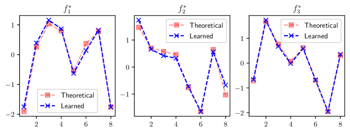
(a) $f_{i}^{*}(x)$ for each $i=1,2,3$

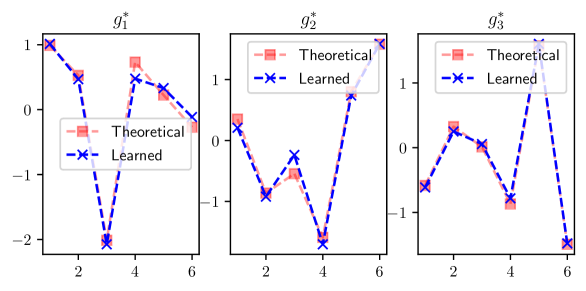
(b) $g_{i}^{*}(y)$ for each $i=1,2,3$

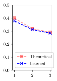
(c) $\sigma_{i}$

Figure 14: Top three dependence modes learned from a discrete dataset, in consistent with theoretical results.

In the experiment, we set $|\mathcal{X}|=8$, $|\mathcal{Y}|=6$, and randomly generate a $P_{X,Y}\in\mathcal{P}^{\mathcal{X}\times\mathcal{Y}}$. We generate $N=30\,000$ training samples from $P_{X,Y}$, and learn $k=3$ dimensional features $f,g$ by maximizing $\mathscr{H}(f,g;\{(1)^{k};\,\mathcal{F}_{\mathcal{X}};\,\mathcal{F}_{\mathcal{Y}}\})$. Then, we normalize each $f_{i},g_{i}$ to obtain corresponding estimations of $f_{i}^{*}$, $g_{i}^{*}$, and $\sigma_{i}$ by applying (40). We show the estimated features and singular values in Figure 14, which are consistent with the corresponding theoretical values computed from $P_{X,Y}$.

7.1.2 Continuous Data

We proceed to consider a continuous dataset with degenerate dependence modes, i.e., the singular values $\sigma_{i}$’s are not all distinct.

In particular, we consider $X,Y$ taking values from $\mathcal{X}=\mathcal{Y}=[-1,1]$, where the joint probability density function $p_{X,Y}$ takes a raised cosine form:

$$p_{X,Y}(x,y)=\frac{1}{4}\cdot\left[1+\cos(\pi(x-y))\right],\quad(x,y)\in[-1,1]^{2}.$$ (100)

Then, it can be verified that the corresponding marginal distributions of $X,Y$ are uniform distributions $p_{X}=p_{Y}=\mathrm{Unif}([-1,1])$. In addition, the resulting CDK function is

$$\mathfrak{i}_{X;Y}(x,y)=\frac{p_{X,Y}(x,y)-p_{X}(x)p_{Y}(y)}{p_{X}(x)p_{Y}(y)} =\cos(\pi(x-y)).$$ (101)

Note that we have $\cos(\pi(x-y))=\cos(\pi x+\theta_{0})\cdot\cos(\pi y+\theta_{0})+\sin(\pi x+\theta_{0})\cdot\sin(\pi y+\theta_{0})$, for any $\theta_{0}\in[-\pi,\pi)$. Therefore, we have $\operatorname{rank}(\mathfrak{i}_{X;Y})=2$, and the associated dependence modes are given by $\sigma_{1}=\sigma_{2}=1/2$ and the maximal correlation functions

$$f_{1}^{*}(x)=\sqrt{2}\cdot\cos(\pi x+\theta_{0}),\qquad f_{2}^{*}(x)=\sqrt{2}\cdot\sin(\pi x+\theta_{0}),$$ (102a)

$$g_{1}^{*}(y)=\sqrt{2}\cdot\cos(\pi y+\theta_{0}),\qquad g_{2}^{*}(y)=\sqrt{2}\cdot\sin(\pi y+\theta_{0}),$$ (102b)

for any $\theta_{0}\in[-\pi,\pi)$.

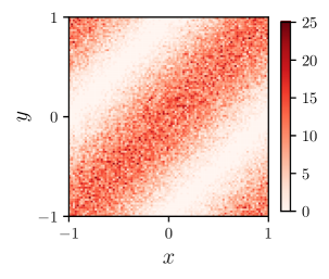
(a) Histogram of Training Data

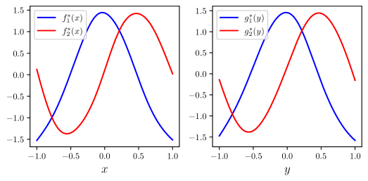
(b) Learned Dependence Modes

Figure 15: Dependence modes learned from continuous data, in consistent with theoretical results.

During this experiment, we first generate $N=50\,000$ sample pairs of $X,Y$ for training, with histogram showing in Figure 15a. Then, we learn $k=2$ dimensional features $f_{1},f_{2}$ of $\mathcal{X}$ and $g_{1},g_{2}$ of $\mathcal{Y}$ by maximizing the nested H-score (38), where $f$ and $g$ are parameterized neural feature extractors detailed in Appendix D.1.2. Figure 15b shows the learned functions after normalization (40). The learned results well match the theoretical results (102): (i) The learned $f_{1}^{*}$ and $f_{2}^{*}$ are sinusoids differ in phase by $\pi/2$, and (ii) $g_{i}^{*}$ coincides with $f_{i}^{*}$, for each $i=1,2$. It is also worth mentioning that due to the degeneracy $\sigma_{1}=\sigma_{2}$, the initial phase $\theta_{0}$ in learned sinusoids (102) can be different during each run of the training algorithm.

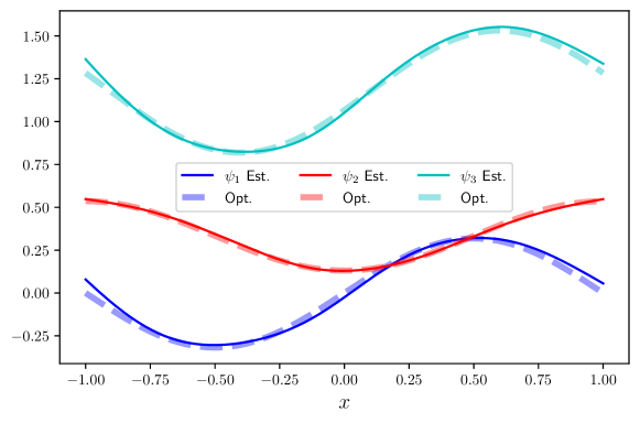
Figure 16: MMSE estimators ${\mathbb{E}}\left[\psi_{i}(Y)|X=x\right]$ obtained from learning dependence modes, in comparison with theoretical results.

Based on the learned dependence modes, we then demonstrate estimating functions of $Y$ based on observed $X=x$. Here, we consider the functions $\psi_{1}(y)=y,\psi_{2}(y)=y^{2},\psi_{3}(y)=e^{y}$. From Proposition 12, we can compute the learned MMSE estimator ${\mathbb{E}}\left[\psi_{i}(Y)|X=x\right]$ for each $i$, by estimating ${\mathbb{E}}\left[\psi_{i}(Y)\right]$ and $\Lambda_{\psi_{i},g}={\mathbb{E}}\left[\psi_{i}(Y)g^{\mathrm{T}}(Y)\right]$ from the training set and then applying (26).

For comparison, we compute the theoretical values

$${\mathbb{E}}\left[\psi_{i}(Y)|X=x\right]=\int_{-1}^{1}p_{Y|X}(y|x)\psi_{i}(y)\,dy,$$

with $p_{Y|X}(y|x)=\frac{1}{2}\cdot\left[1+\cos(\pi(y-x))\right]$, which gives

$${\mathbb{E}}\left[Y\middle|X=x\right]=\frac{1}{\pi}\cdot\sin(\pi x),\qquad\displaystyle{\mathbb{E}}\left[Y^{2}\middle|X=x\right]=\frac{1}{3}-\frac{2}{\pi^{2}}\cos(\pi x),$$ (103a)

$${\mathbb{E}}\left[e^{Y}\middle|X=x\right]=\frac{e^{2}-1}{2e(1+\pi^{2})}\cdot(\pi\sin(\pi x)-\cos(\pi x)+\pi^{2}+1).$$ (103b)

Figure 16 shows the estimators obtained by applying (26) on the learned features, which are consistent with the theoretically optimal estimators given by (103).

7.1.3 Sequential Data

We proceed with an example of learning dependence modes among sequence pairs. For simplicity, we consider binary sequences $\underline{X}$ and $\underline{Y}$, of lengths $l$ and $m$, respectively. Suppose we have the Markov relation $\underline{X}-U-V-\underline{Y}$ for some unobserved binary factors $U,V\in\mathcal{U}=\mathcal{V}=\{0,1\}$. In addition, we assume $\underline{X}=(X_{1},\dots,X_{l})^{\mathrm{T}},\underline{Y}=(Y_{1},\dots,Y_{m})^{\mathrm{T}}$ satisfy

$$\underline{X}|U=i\sim\mathrm{BMS}(l,q_{i}),\quad\underline{Y}|V=i\sim\mathrm{BMS}(m,q_{i}),\quad\text{for $i=0,1$},$$ (104)

where $\mathrm{BMS}(l,q)$ denotes the distribution of a binary first-order Markov sequence of length $l$ and state flipping probability $q$. The corresponding state transition diagram is shown in Figure 17a. Therefore, if $\underline{Z}\sim\mathrm{BMS}(l,q)$, then $Z_{1}\sim\mathrm{Unif}(\{0,1\})$ and $(Z_{1},\dots,Z_{l})$ forms a first order Markov chain over binary states $\{0,1\}$, and flipping probability $\mathbb{P}\left\{Z_{i+1}\neq Z_{i}|Z_{i}=z\right\}=q$ for both $z=0,1$. Formally, $\underline{Z}\sim\mathrm{BMS}(l,q)$ if and only if

$$P_{\underline{Z}}(\underline{z})=\frac{1}{2}\cdot\prod_{i=1}^{l-1}\left[(1-q)^{\delta_{z_{i}z_{i+1}}}\cdot q^{1-\delta_{z_{i}z_{i+1}}}\right]\quad\text{for all $(z_{1},\dots,z_{l})\in\{0,1\}^{l}$}.$$

(a) State Transitions of $\mathrm{BMS}(l,q)$

   

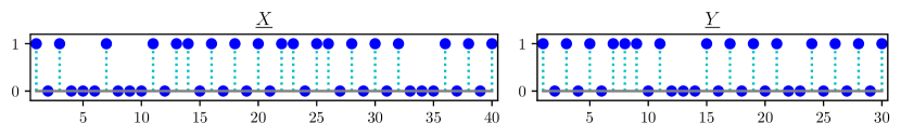
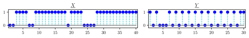
(b) Generated Samples of $\underline{X},\underline{Y}$ Pair

Figure 17: Sequential Data: Model and Generated $\underline{X},\underline{Y}$ Samples Pairs

As a consequence, the resulting alphabets are $\mathcal{X}=\{0,1\}^{l},\mathcal{Y}=\{0,1\}^{m}$, with sizes $|\mathcal{X}|=2^{l},|\mathcal{Y}|=2^{m}$. In our experiment, we set $l=40,m=30,q_{0}=0.1,q_{1}=0.9$, and use the following joint distribution $P_{U,V}$:

Prob.	$U=0$	$U=1$
$V=0$	0.1	0.2
$V=1$	0.4	0.3

We generate $N=50\,000$ training sample pairs of $\underline{X},\underline{Y}$, with instances shown in Figure 17b. We also generate $N^{\prime}=10\,000$ sample pairs in the same manner, as the testing dataset.

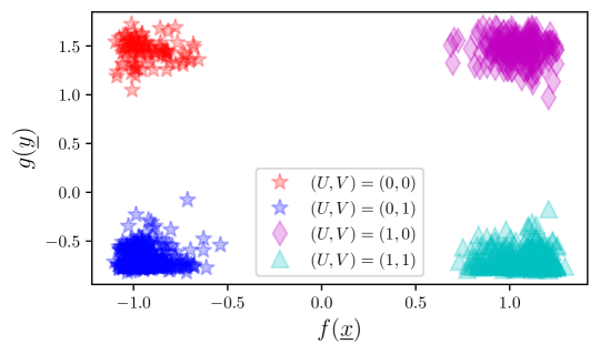
Figure 18: Features Learned from Sequential Data $\underline{X}$ and $\underline{Y}$

Then, we learn $k=1$ dimensional features $f$ and $g$ by maximizing $\mathscr{H}(f,g)$ over the training set. We plot the extracted features in Figure 18. In particular, each point represents an $(f(\underline{x}),g(\underline{y}))$ pair evaluated on an instance from testing set, with corresponding values of binary factors $(U,V)$ shown for comparison. For the ease of demonstration, here we plot only $1,000$ sample pairs randomly chosen from the testing set. As we can see in the figure, the learned features are clustered according to the underlying factors. This essentially reconstructs the hidden factors $U,V$. For example, one can apply a standard clustering algorithm on the features, e.g., $k$-means (Hastie et al., 2009), then count the proportion of each cluster, to obtain an estimation of $P_{U,V}$ up to permutation of symbols.

For a closer inspection, we can compare the learned features with the theoretical results, formalized as follows. A proof is provided in Appendix C.21.

Proposition 36

Suppose $\underline{X},\underline{Y}$ satisfy the Markov relation $\underline{X}-U-V-\underline{Y}$ with $U,V\in\{0,1\}$ and the conditional distributions (104). Then, we have $\operatorname{rank}(\mathfrak{i}_{X;Y})\leq 1$, and the corresponding maximal correlation functions $f_{1}^{*},g_{1}^{*}$ satisfy

$$f_{1}^{*}(\underline{x}) =c\cdot\left[\tanh\left(2w\cdot\varphi(\underline{x})+b_{U}\right)-\tanh(b_{U})\right],$$ (105a)

$$g_{1}^{*}(\underline{y}) =c^{\prime}\cdot\left[\tanh\left(2w\cdot\varphi(\underline{y})+b_{V}\right)-\tanh(b_{V})\right],$$ (105b)

for some $c,c^{\prime}\in\mathbb{R}$, where $w\triangleq\frac{1}{2}\log\frac{q_{1}}{q_{0}},b_{U}\triangleq\frac{1}{2}\log\frac{P_{U}(1)}{P_{U}(0)},b_{V}\triangleq\frac{1}{2}\log\frac{P_{V}(1)}{P_{V}(0)}$, and where we have defined $\varphi\colon\{0,1\}^{*}\to\mathbb{R}$, such that for each $\underline{z}=(z_{1},\dots,z_{l})^{\mathrm{T}}\in\{0,1\}^{l}$, we have $\displaystyle\varphi(\underline{z})\triangleq\frac{l-1}{2}-\sum_{i=1}^{l-1}\delta_{z_{i}z_{i+1}}.$

Then, we compute the correlation coefficients between $f(\underline{X})$ and $f_{1}^{*}(\underline{X})$, and between $g(\underline{Y})$, $g_{1}^{*}(\underline{Y})$, respectively, using sample pairs in the testing set. The absolute values of both correlation coefficients are greater than $0.99$, demonstrating the effectiveness of the learning algorithm.

7.2 Learning With Orthogonality Constraints

We verify the feature learning with orthogonality constraints presented in Section 4.4 on the same dataset used for Section 7.1.2. Here, we consider the settings ${\bar{k}}=k=1$, i.e., we learn one-dimensional feature $f(x)$ uncorrelated to given one dimensional feature $\phi\in\mathcal{F}_{\mathcal{X}}$.

Note that without the orthogonality constraint [cf. (102)], the optimal feature will be sinusoids with any initial phase, i.e., $f_{1}^{*}(x)=\sqrt{2}\cdot\cos(\pi x+\theta_{0})$ for any $\theta_{0}\in[-\pi,\pi)$. Here, we consider the following two choices of $\phi$, $(x\mapsto x)$ and $(x\mapsto x^{2})$, which are even and odd functions, respectively. Since the underlying $p_{X}$ is uniform on $[-1,1]$, we can verify the optimal features under the two constraints are $f^{*}_{1}(x)=\sqrt{2}\cos(\pi x)$ for $\phi(x)=x$, and $f^{*}_{1}(x)=\sqrt{2}\sin(\pi x)$ for $\phi(x)=x^{2}$, respectively.

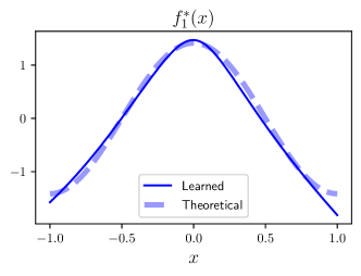
(a) $\phi(x)=x$

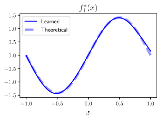
(b) $\phi(x)=x^{2}$

Figure 19: Learning feature uncorrelated to given $\phi$ under different settings of $\phi$. The learned results are compared with theoretical results.

By maximizing the nested H-score restricted to $\bar{f}=\phi$ [cf. (52)], we can learn the optimal feature $f_{1}^{*}$, as shown in Figure 19. The learned features are in consistent with the theoretical ones, validating the effectiveness of the learning algorithm.

7.3 Learning With Side Information

We design an experiment to verify the connection between our learning algorithm and the multitask classification DNN, as demonstrated in Theorem 27.

(a) Learned feature $f(x)$

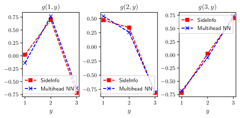
(b) Learned feature $g(s,y)$

Figure 20: Experimental verification of the connection between learning with side information and training a multihead neural network.

In particular, we consider the discrete $X,Y,S$ with $|\mathcal{X}|=8,|\mathcal{S}|=|\mathcal{Y}|=3$, and randomly choose a joint distribution $P_{X,S,Y}$ on $\mathcal{X}\times\mathcal{S}\times\mathcal{Y}$. Then, we generate $N=50\,000$ training samples of $(X,S,Y)$ triples. In our implementation, we set ${\bar{k}}=|\mathcal{S}|-1=2,k=1$ and maximize the nested H-score configured by $\mathcal{C}_{\mathsf{MC}}$ [cf. (59)] on the training set.

For comparison, we also train the multihead network shown in Figure 11 by maximizing the log-likelihood function (70) to learn the corresponding feature $f$ and weight matrices $G_{s}$ for all $s\in\mathcal{S}$. Then, we convert the weights to $g\in\mathcal{F}_{\mathcal{S}\times\mathcal{Y}}$ via the correspondence [cf. (69)] $g(s,y)=G_{s}(1,y)$. The features learned by our algorithm (labeled as “SideInfo”) and the multihead neural network are shown in Figure 20, where the results are consistent.

7.4 Multimodal Learning With Missing Modalities

To verify the multimodal learning algorithms presented in Section 6, we consider multimodal classification problems in two different settings. Suppose $X_{1},X_{2}$ are multimodal data variables, and $Y\in\mathcal{Y}=\{-1,1\}$ denotes the binary label to predict. In the first setting, we consider the training set with complete $(X_{1},X_{2},Y)$ samples. In the second setting, only the pairwise observations of $(X_{1},X_{2})$, $(X_{1},Y)$, and $(X_{2},Y)$ are available, presented in three different datasets.

In both settings, we set $\mathcal{X}_{1}=\mathcal{X}_{2}=[-1,1]$ with

$$P_{X_{1},X_{2}}(x_{1},x_{2})=\frac{1}{4}\cdot\left[1+\cos(2\pi(x_{1}-x_{2}))\right].$$ (106)

We consider predicting $Y$ based on the learned features, where some modality in $X_{1}$, $X_{2}$ might be missing during the prediction.

7.4.1 Learning from Complete Observations

We consider the $X_{1},X_{2},Y$ dependence specified by (106) and the conditional distribution

$$P_{Y|X_{1},X_{2}}(y|x_{1},x_{2})=\frac{1}{2}+\frac{y}{4}\cdot\left[\cos(\pi x_{1})+\cos(\pi x_{2})+\cos(\pi(x_{1}+x_{2}))\right]$$ (107)

for $x_{1},x_{2}\in[-1,1]$ and $y=\pm 1$. It can be verified that $P_{Y}$ satisfies $P_{Y}(1)=P_{Y}(-1)=\frac{1}{2}$. The corresponding CDK function and dependence components [cf. (74)] are given by

$$\mathfrak{i}_{X_{1},X_{2};Y}(x_{1},x_{2},y) =\frac{y}{2}\cdot\left[\cos(\pi x_{1})+\cos(\pi x_{2})+\cos(\pi(x_{1}+x_{2}))\right]$$ (108a)

$$[\pi_{\mathsf{B}}(\mathfrak{i}_{X_{1},X_{2};Y})](x_{1},x_{2},y) =\frac{y}{2}\cdot\left[\cos(\pi x_{1})+\cos(\pi x_{2})\right],$$ (108b)

$$[\pi_{\mathsf{I}}(\mathfrak{i}_{X_{1},X_{2};Y})](x_{1},x_{2},y) =\frac{y}{2}\cdot\cos(\pi(x_{1}+x_{2})).$$ (108c)

Therefore, we have $\operatorname{rank}(\pi_{\mathsf{B}}(\mathfrak{i}_{X_{1},X_{2};Y}))=\operatorname{rank}(\pi_{\mathsf{I}}(\mathfrak{i}_{X_{1},X_{2};Y}))=1$, and the functions obtained from modal decompositions [cf. (91)] are $\bar{g}_{1}^{*}(y)=g_{1}^{*}(y)=y$ and

$$\bar{f}_{1}^{*}(x_{1},x_{2})=\cos(\pi x_{1})+\cos(\pi x_{2}),\qquad f_{1}^{*}(x_{1},x_{2})=\sqrt{2}\cdot\cos(\pi(x_{1}+x_{2})).$$ (109)

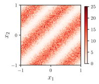
(a) $X_{1},X_{2}$ Histogram

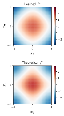
(b) $\bar{f}_{1}^{*}(x_{1},x_{2})$

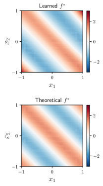
(c) $f_{1}^{*}(x_{1},x_{2})$

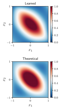
(d) $P_{Y|X_{1},X_{2}}(1|x_{1},x_{2})$

Figure 21: Features and posterior probability learned from multimodal data $X_{1},X_{2},Y$, in comparison with theoretical results.

In the experiment, we first generate $N=50\,000$ triples of $(X_{1},X_{2},Y)$ for training. The histogram of $(X_{1},X_{2})$ pair is shown in Figure 21a. Then, we set ${\bar{k}}=k=1$, and learn the features $\bar{f},f,\bar{g},g$ by maximizing the nested H-score configured by $\mathcal{C}_{\sf BI}$ [cf. (78)]. We then normalize $\bar{f}$, $f$ to obtain the estimated $\bar{f}_{1}^{*}$ and $f_{1}^{*}$, and compute the posterior probability $P_{Y|X_{1},X_{2}}(1|x_{1},x_{2})$ based on (83a). The results of learned features $\bar{f}_{1}^{*}$, $f_{1}^{*}$ and posterior $P_{Y|X_{1},X_{2}}(1|x_{1},x_{2})$ are shown in Figure 21, which are consistent with the theoretical results.

We then consider the prediction problem with missing modality, i.e., predict label $Y$ based on unimodal data $X_{1}$ or $X_{2}$. In particular, based on learned $\bar{f}=\bar{f}^{(1)}+\bar{f}^{(2)}$, we train two separate networks to operate as $\tau_{{1}}$ and $\tau_{{2}}$, then apply (83b) and (83c) to estimate the posteriors $P_{Y|X_{1}}$ and $P_{Y|X_{2}}$. Then, for each $i=1,2$, the MAP prediction of $Y$ based on observed $X_{i}=x_{i}$ can be obtained by comparing $P_{Y|X_{i}}(1|x_{i})$ with the threshold $1/2$, via

$$\operatorname*{arg\,max}_{y\in\mathcal{Y}}P_{Y|X_{i}}(y|x_{i})=\begin{cases}1&\text{if $P_{Y|X_{i}}(1|x_{i})>1/2$},\\ -1&\text{if $P_{Y|X_{i}}(1|x_{i})\leq 1/2$}.\end{cases}$$

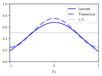
(a) $P_{Y|X_{1}}(1|x_{1})$

(b) $P_{Y|X_{2}}(1|x_{2})$

Figure 22: Label prediction from unimodal data using learned features

We plot the estimated results in Figure 22, in comparison with the threshold $1/2$ and the theoretical values

$$P_{Y|X_{i}}(y|x)=\frac{1}{2}+\frac{y}{4}\cdot\cos(\pi x),\quad\text{for $i=1,2$.}$$ (110)

From the figure, the estimated posteriors $P_{Y|X_{1}},P_{Y|X_{2}}$ have consistent trends with the ground truth posteriors, and the induced $Y$ predictions are well aligned.

7.4.2 Learning from Pairwise Observations

We proceed to consider the multimodal learning with only pairwise observations. Specifically, we consider the joint distribution of $(X_{1},X_{2},Y)$, specified by (106) and

$$P_{Y|X_{1},X_{2}}(y|x_{1},x_{2})=\frac{1}{2}+\frac{y}{4}\cdot\left[\cos(\pi x_{1})+\cos(\pi x_{2})\right].$$ (111)

for $x_{1},x_{2}\in[-1,1]$ and $y=\pm 1$. It can be verified that $P_{Y}(1)=P_{Y}(-1)=\frac{1}{2}$, and the associated CDK function satisfies

$$\mathfrak{i}_{X_{1},X_{2};Y}(x_{1},x_{2},y)=\frac{y}{2}\cdot\left[\cos(\pi x_{1})+\cos(\pi x_{2})\right].$$ (112)

and $\mathfrak{i}_{X_{1},X_{2};Y}=\pi_{\mathsf{B}}(\mathfrak{i}_{X_{1},X_{2};Y})$. Therefore, the interaction dependence component $\pi_{\mathsf{I}}(\mathfrak{i}_{X_{1},X_{2};Y})=0$, and the joint dependence can be learned from all pairwise samples, as we discussed in Section 6.5.1.

We then construct an experiment to verify learning joint dependence from all pairwise observations. Specifically, we generate $N=50\,000$ triples of $(X_{1},X_{2},Y)$ from (106) and (111). Then, we adopt the decomposition (89) on each triple, to obtain three pairwise datasets with samples of $(X_{1},X_{2})$, $(X_{1},Y)$, $(X_{2},Y)$, where each dataset has $N$ sample pairs.

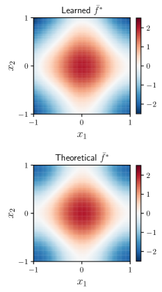
(a) $\bar{f}_{1}^{*}(x_{1},x_{2})$

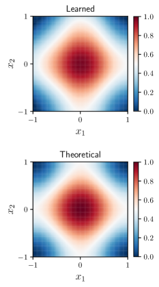
(b) $P_{Y|X_{1},X_{2}}(1|x_{1},x_{2})$

Figure 23: Features and posterior probability learned from pairwise datasets of $(X_{1},X_{2}),(X_{1},Y)$, and $(X_{2},Y)$, in comparison with theoretical results.

We use these three pairwise datasets for training to learn one dimensional $\bar{f}\in\mathcal{F}_{\mathcal{X}},\bar{g}\in\mathcal{F}_{\mathcal{Y}}$ that maximize $\mathscr{H}(\bar{f},\bar{g})$. Here, we compute $\mathscr{H}(\bar{f},\bar{g})$ based on the minibatches from the three pairwise datasets, according to (93). Based on learned $\bar{f},\bar{g}$, we then compute the normalized $\bar{f}_{1}^{*}$ and posterior distribution $P_{Y|X_{1},X_{2}}(1|x_{1},x_{2})$, as shown in Figure 23, where the learned results match the theoretical values.

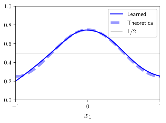
(a) $P_{Y|X_{1}}(1|x_{1})$

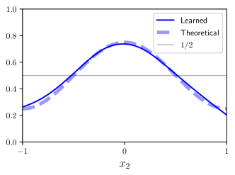
(b) $P_{Y|X_{2}}(1|x_{2})$

Figure 24: Label prediction from unimodal data, with features learned from pairwise datasets.

Similar to the previous setting, we consider the unimodal prediction problem, and show the estimated results in Figure 24. It is worth noting that from (108b), (112), the joint distributions $P_{X_{1},X_{2},Y}$ in both settings contain the same bivariate dependence component. Therefore, the theoretical results for $\bar{f}_{1}^{*}$ and $P_{Y|X_{1}},P_{Y|X_{2}}$ are the same.

8 Related Works

Maximal Correlation Functions: Optimality, Learning Algorithms, and Applications

The Hirschfeld–Gebelein–Rényi (HGR) maximal correlation (Hirschfeld, 1935; Gebelein, 1941; Rényi, 1959) provides an important connection between statistical dependence and function space. The same concept has been studied with various formulations, and often in different terminologies, such as correspondence analysis (Greenacre, 2017), functional canonical variates (Buja, 1990), and principal inertial components (du Pin Calmon et al., 2017). See, e.g., (Huang et al., 2019, Section II), for a detailed discussion. The optimality of HGR maximal correlation functions has been extensively studied in literature, e.g., as the optimal transformations in regression problems Breiman and Friedman (1985); Buja (1990). In particular, if one variable is categorical and represents the class label, the maximal correlation functions also provide the best inter-class separability (Xu and Huang, 2020, Section III-B). The maximal correlation functions also play a fundamental role in the discussion of informative feature extraction and local information geometry, as we will detail next. The first practical algorithm for learning such functions is the alternating conditional expectations (ACE) algorithm (Breiman and Friedman, 1985; Buja, 1990), which learns the top dependence mode and are mostly used for processing low-dimensional data. To tackle high-dimensional data, recent developments focused on learning maximal correlation functions by DNNs. Specifically, the H-score was derived from the low-rank approximation of the canonical dependence kernel, referred as the Soft-HGR objective (Wang et al., 2019). It was also introduced as the local approximation of the log loss function (Xu et al., 2022), as we have discussed in Section 3.4. In an independent line of work (HaoChen et al., 2021), a special form of H-score was proposed for self-supervised learning tasks, referred to as the spectral contrastive loss therein. There are also other formulations and algorithms proposed for computing the maximal correlation functions; see, e.g., Andrew et al. (2013) and Hsu et al. (2021). Compared to the low-rank approximation formulation, such approaches typically require explicit whitening procedures or computations of matrix inverses, which are less applicable for learning high-dimensional features. The sample complexity for learning maximal correlation functions have been investigated recently; see, e.g., Huang and Xu (2020); Makur et al. (2020). The maximal correlation learning, particularly the H-score maximization formulation, has been widely applied in feature extraction for multimodal data, e.g., Wang et al. (2019) and the follow-up works. For example, Xu and Huang (2020) developed maximal correlation regression (MCR), which applied learned maximal correlation functions for solving classification tasks.

Informative Feature Extraction and Local Information Geometry

Huang et al. (2019) has provided an in-depth characterization of informative features by applying information-theoretic tools, with a focus on bivariate learning problems and the local analysis regime. Under such settings, it was shown that a series of statistical and learning formulations leading to the same optimal features, characterized as the HGR maximal correlation functions. Examples of these formulations include the information bottleneck Tishby et al. (2000) and a cooperative game. There are similar information-theoretic discussions on multivariate problems. For example, Xu and Zheng (2022) presented the information-theoretic optimality of the features defined in (66). The features introduced in (91a) were also studied by Xu and Huang (2021) in characterizing distributed hypothesis testing problems.

Decomposition of Probability Distributions

The decomposition of probability distributions has been studied, particularly in the context of information geometry (Amari and Nagaoka, 2000). For example, Amari (2001) established a decomposition in distribution space, which also investigated the maximum entropy formulation (87), cf. (Amari, 2001, Theorem 7). The information geometry induced by classification DNNs, with softmax activation and log loss function, was investigated in Xu et al. (2018), which corresponds to the optimal features for Proposition 14 without the weak dependence assumption.

The geometric framework we presented is built upon these existing works and the perspectives from information theory, statistical analysis, and machine learning. The key component is a unified geometric view of feature learning design, which has provided nontrivial extensions to existing works. In particular, with the geometric viewpoint and nesting technique, we have developed general operations of multivariate statistical dependence, with the existing bivariate learning algorithm (Wang et al., 2019; Xu and Huang, 2020) being atom operations and special cases. Our developments have also revealed the learning implications of existing theoretical developments, e.g., Amari and Nagaoka (2000) and Huang et al. (2019).

9 Conclusions and Discussion

We have presented a framework for designing learning systems with neural feature extractors, which allows us to learn informative features and assemble them to build different inference models. Based on the feature geometry, we use feature representations as the interface, and convert learning problems to corresponding geometric operations in feature spaces. We then introduce the nesting technique for implementing such geometric operations in feature spaces, which provides a systematic design of both feature learning and feature assembling modules. We demonstrate its applications in learning multivariate dependence by considering conditioned inference and multimodal learning problems.

The developed framework has provided a unified solution to general feature-centric learning problems, where we have utilized DNNs as building blocks to learn features that best represent the statistical dependence. The connection between feature and statistical dependence enables principled learning algorithm designs, especially in multivariate learning scenarios. Such designs also provide a learning-based computational approach for investigating the statistical dependence behind high-dimensional data with often complicated structures.

9.1 Applications and Extensions

For simplicity, our presentation focused on theoretical concepts and basic settings, which can be readily applied to practical learning scenarios and extended to more complicated settings. For instance, we can establish the feature optimality in multivariate problems by extending the bivariate characterizations (Huang et al., 2019; Xu and Huang, 2020); see, e.g, the discussions in Xu and Zheng (2022).

For applications, the results in Proposition 12 can be applied to classification and estimation tasks, e.g., image classification (Xu and Huang, 2020). Similarly, we can employ the results in Section 4.4 to address physical or engineering constraints induced by practical learning applications. We can also apply the learning framework to process multimodal data dependencies and learn useful features, as discussed in Section 5 and Section 6. We can incorporate pre-trained models to reduce data requirements and computational costs for all such examples.

Our discussions on the dependence decomposition framework can also be extended to general settings. In particular, we can get refined dependence components by iteratively applying the decomposition (43). One example is to decompose the dependence of a random processes into different dependence components, with each component representing the dependence at a certain time delay, as discussed in Xu and Zheng (2023b). More generally, the nesting technique can be extended by considering a configurations (cf. Definition 16) with subspace sequences of both $\mathcal{F}_{\mathcal{X}}$ and $\mathcal{F}_{\mathcal{Y}}$.

We can also extend our discussions and analyses on supervised learning examples to other scenarios, e.g., contrastive (Chen et al., 2020) and self-supervised (HaoChen et al., 2021) learning problems. In addition to the neural feature extractors, the feature geometry can also be applied to implicit features, e.g., the feature subspaces in kernel methods. In particular, Xu and Zheng (2023a) developed a quantitative measure of kernel choices and demonstrated a connection between kernel methods and existing feature learning approaches.

9.2 Future Directions

The established framework provides abundant opportunities for further explorations in both theoretical analyses and applications. To highlight the general framework, our development has adopted simplified or idealized assumptions on learning factors, e.g., the network expressive power. By relaxing such idealized assumptions, further investigations can give a better theoretical understanding and also provide practical guidance. Preliminary examples include our discussions on the expressive power of feature extractors (cf. Section 3.3) and the sample size of training data (cf. Section 6.5.2). More in-depth characterizations on the learning behaviors, e.g., generalizability, can be built upon the spectrum decomposition nature of this learning framework, by utilizing existing analyses on linear operators (Dunford and Schwartz, 1988) or the spectral methods for matrices (Chen et al., 2021). Another interesting direction is to investigate the interaction between feature geometry, the manifold structure of the neural feature extractor, and the geometry of data spaces (Bronstein et al., 2017, 2021). Moreover, the nested H-score and the induced optimization behaviors can be of independent interest to optimization studies, e.g., the landscape and convergence analyses. In terms of applications, the established framework can be extended to other operations on statistical dependence beyond decomposing or learning given dependence. For instance, a potential application is to generate data satisfying certain dependence constraints, e.g., independence or conditional independence, by employing generative models. The integration with generative models, as well as the learning algorithm design, is of practical interest for further studies.

Acknowledgments and Disclosure of Funding

This work was supported in part by the National Science Foundation (NSF) under Award CNS-2002908 and the Office of Naval Research (ONR) under grant N00014-19-1-2621.

Appendix A Data Alphabets in Feature Geometry

We discuss the feature geometry on general data alphabets, e.g., continuous alphabets in Appendix A.1. In Appendix A.2, we briefly summarize the vector and matrix notation conventions established for discrete alphabets, which have been extensively used in related works, e.g., Huang et al. (2019); Xu et al. (2022).

A.1 General Alphabets: Regularity Conditions and Examples

Our development on feature spaces can be extended to general Hilbert spaces (Young, 1988; Weidmann, 2012), where the alphabet $\mathcal{Z}$ and the metric distribution $P_{Z}$ (cf. Section 2.1.2) are extended to a measurable set and the measure (Weidmann, 2012, Example 6), respectively.

One particularly important example is $\mathcal{Z}=\mathbb{R}^{d}$ with $d\geq 1$. We consider the random variable $\underline{Z}\in\mathcal{Z}$. For simplicity, we restrict to the case where $\underline{Z}$ has the probability density function $p_{\underline{Z}}$. Then, we define the feature space $\mathcal{F}_{\mathcal{Z}}$ and the inner product on $\mathcal{F}_{\mathcal{Z}}$ as [cf. Section 2.1.2]

$$\mathcal{F}_{\mathcal{Z}}\triangleq\left\{f\colon\mathcal{Z}\to\mathbb{R},\int f^{2}(\underline{z})p_{\underline{Z}}(\underline{z})d\underline{z}<\infty\right\},\quad\text{and}\quad\langle f_{1},f_{2}\rangle\triangleq\int f_{1}(\underline{z})f_{2}(\underline{z})p_{\underline{Z}}(\underline{z})d\underline{z}\text{ for }f_{1},f_{2}\in\mathcal{F}_{\mathcal{Z}},$$

respectively.

We can define the joint function similarly for $\mathcal{X}$, $\mathcal{Y}$ under the corresponding regularity conditions. For instance, we consider $(X,Y)$ with alphabets $\mathcal{X}=\mathcal{Y}=\mathbb{R}$ and the joint probability density function $p_{X,Y}$. Then, the corresponding definition of the CDK function becomes [cf. (4)]

$$\mathfrak{i}_{X;Y}(x,y)=\frac{p_{X,Y}(x,y)}{p_{X}(x)p_{Y}(y)}-1.$$ (113)

Note that to have $\mathfrak{i}_{X;Y}\in\mathcal{F}_{\mathcal{X}\times\mathcal{Y}}$, we need to assume

$$\|\mathfrak{i}_{X;Y}\|^{2}=\iint\frac{[p_{X,Y}(x,y)]^{2}}{p_{X}(x)p_{Y}(y)}\,dxdy-1<\infty,$$ (114)

where the norm is defined with respect to the metric distribution $p_{X}p_{Y}$.

Remark 37

The results can be further generalized to the case where density functions not necessarily exist. See, e.g., Lancaster (1958) and (Buja, 1990, Proposition 3.1) for detailed discussions.

In particular, we have the following result for bivariate normal variables, which has been extensively discussed in literature; see, e.g., Lancaster (1958) and Huang et al. (2019).

Example 2

For bivariate normal variables $\begin{bmatrix}X\\ Y\end{bmatrix}\sim\mathcal{N}\left(\begin{bmatrix}0\\ 0\end{bmatrix},\begin{bmatrix}1&\rho\\ \rho&1\end{bmatrix}\right)$ with $|\rho|<1$, we have

$$\mathfrak{i}_{X;Y}(x,y)=\sum_{i=1}^{\infty}\frac{\rho^{i}}{i!}\cdot\mathtt{He}_{i}(x)\cdot\mathtt{He}_{i}(y).$$ (115)

where for each $i\geq 1$, $\mathtt{He}_{i}$ denotes the $i$-th (probabilist’s) Hermite polynomial, defined as

$$\mathtt{He}_{i}(x)\triangleq(-1)^{i}\cdot e^{\frac{x^{2}}{2}}{\frac{d^{i}}{dx^{i}}}e^{-{\frac{x^{2}}{2}}}.$$

Then, each $i$-th mode of $\mathfrak{i}_{X;Y}$ can be written in the standard form as $\operatorname{\zeta}_{i}(\mathfrak{i}_{X;Y})=\sigma_{i}(f_{i}^{*}\otimes g_{i}^{*})$, with

$$\sigma_{i}=|\rho|^{i},\quad f_{i}^{*}=\frac{1}{\sqrt{i!}}\cdot\mathtt{He}_{i},\quad g_{i}^{*}=\frac{[\operatorname{sgn}(\rho)]^{i}}{\sqrt{i!}}\cdot\mathtt{He}_{i}.$$ (116)

Finally, $\displaystyle\|\mathfrak{i}_{X;Y}\|^{2}=\sum_{i\geq 1}\sigma_{i}^{2}=\frac{\rho^{2}}{1-\rho^{2}}$.

The equation (115) is referred to as Mehler’s identity or Mehler’s decomposition (Mehler, 1866).

In some scenarios, $\mathcal{X}$ and $\mathcal{Y}$ can be of different types, e.g., $\mathcal{X}$ is continuous, and $\mathcal{Y}$ is discrete. A classical example is mixture model, where $X$ and $Y$ corresponds to the observation variable and the latent categorical variable, respectively. Specifically, we introduce the following Gaussian mixture example, which is a multidimensional extension of an example discussed in Buja (1990).

Example 3

We consider the probability model with $\mathcal{Y}=\{1,-1\}$, $P_{Y}\equiv\frac{1}{2}$, and $\underline{X}|Y=y\sim\mathcal{N}(y\cdot\underline{\mu},\Sigma)$ for $y\in\mathcal{Y}$, where $\underline{\mu}\in\mathbb{R}^{d}$ and $\Sigma$ is a positive definite matrix of order $d$, for some $d\geq 1$. Then, we have $\operatorname{rank}(\mathfrak{i}_{\underline{X};Y})=1$ with the standard form $\mathfrak{i}_{\underline{X};Y}=\sigma_{1}(f_{1}^{*}\otimes g_{1}^{*})$, where $g_{1}^{*}(y)=y$ and $f_{1}^{*}(\underline{x})=c\cdot\tanh(\underline{\mu}^{\mathrm{T}}\Sigma^{-1}\underline{x})$ for some $c\in\mathbb{R}$.

Proof  We have

$$\mathfrak{i}_{\underline{X};Y}(\underline{x},y) =\frac{p_{\underline{X}|Y}(\underline{x}|y)}{p_{\underline{X}}(\underline{x})}-1$$

$$=2\cdot\frac{\exp(-\frac{1}{2}(\underline{x}-y\underline{\mu})^{\mathrm{T}}\Sigma^{-1}(\underline{x}-y\underline{\mu}))}{\exp(-\frac{1}{2}(\underline{x}+\underline{\mu})^{\mathrm{T}}\Sigma^{-1}(\underline{x}+\underline{\mu}))+\exp(-\frac{1}{2}(\underline{x}-\underline{\mu})^{\mathrm{T}}\Sigma^{-1}(\underline{x}-\underline{\mu}))}-1$$

$$=\frac{2\exp(y\underline{\mu}^{\mathrm{T}}\Sigma^{-1}\underline{x})}{\exp(\underline{\mu}^{\mathrm{T}}\Sigma^{-1}\underline{x})+\exp(-\underline{\mu}^{\mathrm{T}}\Sigma^{-1}\underline{x})}-1$$

$$=y\cdot\frac{\exp(\underline{\mu}^{\mathrm{T}}\Sigma^{-1}\underline{x})-\exp(-\underline{\mu}^{\mathrm{T}}\Sigma^{-1}\underline{x})}{\exp(\underline{\mu}^{\mathrm{T}}\Sigma^{-1}\underline{x})+\exp(-\underline{\mu}^{\mathrm{T}}\Sigma^{-1}\underline{x})}$$

$$=y\cdot\tanh(\underline{\mu}^{\mathrm{T}}\Sigma^{-1}\underline{x}),$$

which implies that $\operatorname{rank}(\mathfrak{i}_{\underline{X};Y})=1$, $f_{1}^{*}(\underline{x})\propto\tanh(\underline{\mu}^{\mathrm{T}}\Sigma^{-1}\underline{x})$, and $g_{1}^{*}(y)=y$.  

From Example 3, the maximal correlation function $f_{1}^{*}$ can be represented by a $d\times 1$ linear layer activated by $\tanh(\cdot)$, with zero bias and weight $\Sigma^{-1}\underline{\mu}$.

A.2 Finite Alphabets: Information Vector and Canonical Dependence Matrix

For finite data alphabets, it can be convenient to introduce the vector and matrix representations of features. To begin, we assume the random variable $Z$ takes finite many possible values, i.e., $|\mathcal{Z}|<\infty$, then the resulting feature space $\mathcal{F}_{\mathcal{Z}}$ is a finite-dimensional vector space. It is sometimes more convenient to represent features using vector and matrix notations. Specifically, each $f\in\mathcal{F}_{\mathcal{Z}}$ can be equivalently expressed as one vector in $\mathbb{R}^{|\mathcal{Z}|}$ as follows. Suppose $R_{Z}$ is the metric distribution, then we can construct an orthonormal basis $\left\{\mathsf{b}_{Z}^{(z)}\colon z\in\mathcal{Z}\right\}$ of $\mathcal{F}_{\mathcal{Z}}$, where

$$\mathsf{b}_{Z}^{(z)}(z^{\prime})\triangleq\frac{\delta_{zz^{\prime}}}{\sqrt{R_{Z}(z)}}\quad\text{for all $z,z^{\prime}\in\mathcal{Z}$}.$$ (117)

We refer to this basis as the canonical basis of $\mathcal{F}_{\mathcal{Z}}$. For all $f\in\mathcal{F}_{\mathcal{Z}}$, we can represent $f$ as a linear combination of these basis functions, i.e.,

$$f=\sum_{z^{\prime}\in\mathcal{Z}}\xi(z^{\prime})\cdot\mathsf{b}_{Z}^{(z^{\prime})},$$

where the coefficient $\xi(z)$ for each $z\in\mathcal{Z}$ is given by

$$\xi(z)=\left\langle f,\mathsf{b}_{Z}^{(z)}\right\rangle=f(z)\sqrt{R_{Z}(z)}.$$ (118)

In particular, when $f$ is the density ratio $\tilde{\ell}_{P_{Z}}$ for some $P_{Z}\in\mathcal{F}_{\mathcal{Z}}$, the corresponding coefficient $\xi(z)$ for each $z\in\mathcal{Z}$ is

$$\xi(z)=\left\langle\tilde{\ell}_{P_{Z}},\mathsf{b}_{Z}^{(z)}\right\rangle=\frac{P_{Z}(z)-R_{Z}(z)}{\sqrt{R_{Z}(z)}}.$$ (119)

This establishes a one-to-one correspondence between $\tilde{\ell}_{P_{Z}}$ (or $P_{Z}$) and the vector $\underline{\xi}\triangleq[\xi(z),z\in\mathcal{Z}]^{\mathrm{T}}\in\mathbb{R}^{|\mathcal{Z}|}$, which is referred to as the information vector associated with $\tilde{\ell}_{P_{Z}}$ (or $P_{Z}$).

Similarly, for $X$ and $Y$ with $|\mathcal{X}|<\infty,|\mathcal{Y}|<\infty$, we can represent the CDK function $\mathfrak{i}_{X;Y}\in\mathcal{F}_{\mathcal{X}\times\mathcal{Y}}$ as an $|\mathcal{X}|\times|\mathcal{Y}|$ matrix $\tilde{B}_{X;Y}$:

$$\tilde{B}_{X;Y}(x;y) \triangleq\frac{P_{X,Y}(x,y)-P_{X}(x)P_{Y}(y)}{\sqrt{P_{X}(x)}\sqrt{P_{Y}(y)}},$$ (120)

which is referred to as the canonical dependence matrix (CDM) of $X$ and $Y$. With the metric distribution $P_{X}P_{Y}$ on $\mathcal{F}_{\mathcal{X}\times\mathcal{Y}}$, each $\tilde{B}_{X;Y}(x;y)$ is the coefficient associated with the basis function $\mathsf{b}_{X,Y}^{(x,y)}$ [cf. (117)].

In addition, we have $\operatorname{rank}(\tilde{B}_{X;Y})=\operatorname{rank}(\mathfrak{i}_{X;Y})$. Suppose $\sigma_{i}(f_{i}^{*}\otimes g_{i}^{*})=\operatorname{\zeta}_{i}(\mathfrak{i}_{X;Y})$, for each $1\leq i\leq\operatorname{rank}(\mathfrak{i}_{X;Y})$, then $\sigma_{i}$ is the $i$-th singular vector of $\tilde{B}_{X;Y}$, and the corresponding $i$-th left and right singular vector pair are given by $\underline{\xi}_{i}^{X}\in\mathbb{R}^{|\mathcal{X}|},\underline{\xi}_{i}^{Y}\in\mathbb{R}^{|\mathcal{Y}|}$, with [cf. (118)]

$$\xi_{i}^{X}(x)=\sqrt{P_{X}(x)}\cdot f_{i}^{*}(x),\quad\xi_{i}^{Y}(y)=\sqrt{P_{Y}(y)}\cdot g_{i}^{*}(y).$$ (121)

Therefore, for small-scale discrete data, we can use the connection (121) to obtain the modal decomposition by solving the SVD of the corresponding CDM.

Appendix B Characterization of Common Optimal Solutions

We consider optimization problems defined on a common domain $\mathcal{D}$. Specifically, given $k$ functions $h_{i}\colon\mathcal{D}\to\mathbb{R}$, $i=1,\dots,k$, let us consider optimization problems

$$\operatorname*{maximize}_{u\in\mathcal{D}}h_{i}(u),\quad i=1,\dots,k.$$ (122)

For each $i=1,\dots,k$, we denote the optimal solution and optimal value for $i$-th problem by

$$\mathcal{D}_{i}^{*}\triangleq\operatorname*{arg\,max}_{u\in\mathcal{D}}h_{i}(u),\quad t_{i}^{*}\triangleq\max_{u\in\mathcal{D}}h_{i}(u),$$ (123)

respectively, and suppose $\mathcal{D}_{i}^{*}\neq\varnothing,i=1,\dots,k$.

Then, the set $\mathcal{D}^{*}\triangleq\cap_{i=1}^{k}\mathcal{D}_{i}^{*}$ represents the collection of common optimal solutions for all $k$ optimization problems (122). When such common solutions exist, i.e., $\mathcal{D}^{*}$ is nonempty, we can obtain $\mathcal{D}^{*}$ by a single optimization program, by using an objective that aggregates original $k$ objectives. We formalize the result as follows.

Proposition 38

If $\mathcal{D}^{*}\neq\varnothing$, we have $\displaystyle\mathcal{D}^{*}=\operatorname*{arg\,max}_{u\in\mathcal{D}}\,\Gamma(h_{1}(u),h_{2}(u),\dots,h_{k}(u))$ for every $\Gamma\colon\mathbb{R}^{k}\to\mathbb{R}$ that is strictly increasing in each argument.

Proof  Let $\mathcal{D}^{**}\triangleq\operatorname*{arg\,max}_{u\in\mathcal{D}}\,h(u)$ with $h(u)\triangleq\Gamma(h_{1}(u),h_{2}(u),\dots,h_{k}(u))$. Then the proposition is equivalent to $\mathcal{D}^{*}=\mathcal{D}^{**}$. We then establish $\mathcal{D}^{*}\subset\mathcal{D}^{**}$ and $\mathcal{D}^{**}\subset\mathcal{D}^{*}$, respectively.

To prove $\mathcal{D}^{*}\subset\mathcal{D}^{**}$, take any $u^{*}\in\mathcal{D}^{*}$. Then, for all $u\in\mathcal{D}$, we have $h_{i}(u)\leq h_{i}(u^{*})$, $i=1,\dots,k$, which implies that

$$h(u)=\Gamma(h_{1}(u),\dots,h_{k}(u))\leq\Gamma(h_{1}(u^{*}),\dots,h_{k}(u^{*}))=h(u^{*}).$$

Therefore, we have $u^{*}\in\mathcal{D}^{**}$. Since $u^{*}$ can be arbitrarily chosen from $\mathcal{D}^{*}$, we have $\mathcal{D}^{*}\subset\mathcal{D}^{**}$.

We then establish $\mathcal{D}^{**}\subset\mathcal{D}^{*}$, which is equvialent to

$$(\mathcal{D}\setminus\mathcal{D}^{*})\subset(\mathcal{D}\setminus\mathcal{D}^{**}).$$ (124)

Note that (124) is trivially true if $\mathcal{D}\setminus\mathcal{D}^{*}=\varnothing$. Otherwise, take any $u^{\prime}\in\mathcal{D}\setminus\mathcal{D}^{*}$. Then, we have $h_{i}(u^{\prime})\leq h_{i}(u^{*})$ for all $i\in[k]$, and the strict inequality holds for at least one $i\in[k]$. This implies that

$$h(u^{\prime})=\Gamma(h_{1}(u^{\prime}),\dots,<h_{k}(u^{\prime}))<\Gamma(h_{1}(u^{*}),\dots,h_{k}(u^{*}))=h(u^{*}).$$

Hence, $u^{\prime}\notin\mathcal{D}^{**}$, and thus $u^{\prime}\in(\mathcal{D}\setminus\mathcal{D}^{**})$, which establishes (124).  

To apply Proposition 38, the first step is to test the existence of common optimal solutions. A naive test is to solve all optimization problems (122) and then check the definition, which can be difficult in practice. Instead, we can consider a related multilevel optimization problem as follows. Let $\mathcal{D}_{0}\triangleq\mathcal{D}$, and for each $i=1,\dots,k$ as, we define $\mathcal{D}_{i}$ and $t_{i}\in\mathbb{R}$ as

$$\mathcal{D}_{i}\triangleq\operatorname*{arg\,max}_{u\in\mathcal{D}_{\!i-1}}\,h_{i}(u),\quad t_{i}\triangleq\max_{u\in\mathcal{D}_{\!i-1}}\,h_{i}(u).$$ (125)

Note that for each $i$, the $\mathcal{D}_{i}$ solved by level $i$ optimization problem gives the elements in $\mathcal{D}_{i}$ that maximize $h_{i}$, and $t_{i}$ denotes the corresponding optimal value. Therefore, $\mathcal{D}_{k}$ can be obtained by sequentially solving $k$ optimization problems as defined in (125).

Then, the following result provides an approach to test the existence of common optimal solutions.

Proposition 39

The following three statements are equivalent:

1. The optimization problems (122) have common optimal solutions, i.e., $\mathcal{D}^{*}\neq\varnothing$;

2. $t_{i}=t_{i}^{*}$ for all $i=1,\dots,k$;

3. $\mathcal{D}_{i-1}\cap\mathcal{D}_{i}^{*}\neq\varnothing$ for all $i=1,\dots,k$.

In addition, if one of these statements holds, then we have $\mathcal{D}_{k}=\mathcal{D}^{*}$.

Proof  We establish the equivalence of the statements 1 to 3, by showing that “1” $\implies$ “2”, “2” $\implies$ “3”, and “3” $\implies$ “1”.

“1” $\implies$ “2”

Suppose “1” holds, and take any $u^{*}\in\mathcal{D}^{*}=\cap_{i=1}^{k}\mathcal{D}_{i}^{*}$. We then establish “2” by induction. First, note that $u^{*}\in\mathcal{D}_{0}$. For the induction step, we can show that for each $i=1,\dots,k$, if $u^{*}\in\mathcal{D}_{i-1}$, then $u^{*}\in\mathcal{D}_{i}$ and $t_{i}^{*}=t_{i}$. Indeed, we have

$$t_{i}^{*}\geq t_{i}=\max_{u\in\mathcal{D}_{i-1}}h_{i}(u)\geq h_{i}(u^{*})=t_{i}^{*},$$

where the first inequality follows from the fact that $\mathcal{D}=\mathcal{D}_{0}\supset\mathcal{D}_{1}\supset\dots\supset\mathcal{D}_{k}$, where the second inequality follows from the inductive assumption $u^{*}\in\mathcal{D}_{i-1}$, and where the last equality follows from that $u^{*}\in\mathcal{D}^{*}\subset\mathcal{D}_{i}^{*}$.

“2” $\implies$ “3”

For each $i=2,\dots,k$, $t_{i}=t_{i}^{*}$ implies that there exists some $u_{i}\in\mathcal{D}_{i-1}$, such that $h_{i}(u_{i})=t_{i}=t_{i}^{*}=\max_{u\in\mathcal{D}}h_{i}(u)$, and thus $u_{i}\in\mathcal{D}_{i}^{*}$. Therefore, $u_{i}\in\mathcal{D}_{i-1}\cap\mathcal{D}_{i}^{*}$, which establishes “3”.

“3” $\implies$ “1”

For each $i=2,\dots,k$, from $\mathcal{D}_{i-1}\cap\mathcal{D}_{i}^{*}\neq\varnothing$ and the definitions (123) and (125), we have $\mathcal{D}_{i}=\mathcal{D}_{i-1}\cap\mathcal{D}_{i}^{*}$. It can also be verified that $\mathcal{D}_{i}=\mathcal{D}_{i-1}\cap\mathcal{D}_{i}^{*}$ holds for $i=1$. Therefore, we obtain

$$\mathcal{D}_{k}=\mathcal{D}_{k-1}\cap\mathcal{D}_{k}^{*}=\mathcal{D}_{k-2}\cap\mathcal{D}_{k-1}^{*}\cap\mathcal{D}_{k}^{*}=\dots=\mathcal{D}_{0}\cap\left(\bigcap_{i=1}^{k}\mathcal{D}_{i}^{*}\right)=\mathcal{D}\cap\mathcal{D}^{*}=\mathcal{D}^{*}.$$ (126)

This implies that $\mathcal{D}^{*}=\mathcal{D}_{k-1}\cap\mathcal{D}_{k}^{*}\neq\varnothing$.

Finally, from (126) we know that statement 3 implies $\mathcal{D}_{k}=\mathcal{D}^{*}$. Since all three statements are equivalent, each statement implies $\mathcal{D}_{k}=\mathcal{D}^{*}$.  

Appendix C Proofs

C.1 Proof of Proposition 5

Let $\hat{\gamma}\triangleq\Pi\left(\gamma;{\mathcal{G}_{\mathcal{X}}\otimes\mathcal{G}_{\mathcal{Y}}}\right)$. We first consider the second equality of (18), i.e.,

$$\operatorname{\zeta}_{\leq k}(\hat{\gamma})=\operatorname*{arg\,min}_{\begin{subarray}{c}\gamma^{\prime}\colon\gamma^{\prime}=f\otimes g,\\ f\in\mathcal{G}_{\mathcal{X}}^{\,k},\,g\in\mathcal{G}_{\mathcal{Y}}^{\,k}\end{subarray}}\|\gamma-\gamma^{\prime}\|$$ (127)

For each $k\leq\operatorname{rank}(\hat{\gamma})$, consider $\gamma^{\prime}=f\otimes g$ with $f\in\mathcal{G}_{\mathcal{X}}^{\,k},g\in\mathcal{G}_{\mathcal{Y}}^{\,k}$. Then, we have

$$\|\gamma-\gamma^{\prime}\|^{2}=\|\gamma-\hat{\gamma}+\hat{\gamma}-\gamma^{\prime}\|^{2}=\|\gamma-\hat{\gamma}\|^{2}+\|\hat{\gamma}-\gamma^{\prime}\|^{2}\geq\|\gamma-\hat{\gamma}\|^{2}+\|r_{k}(\hat{\gamma})\|^{2},$$ (128)

where to obtain the second equality we have used the orthogonality principle with fact that $(\gamma-\hat{\gamma})\perp\mathcal{G}_{\mathcal{X}}\otimes\mathcal{G}_{\mathcal{Y}}$ and $(\hat{\gamma}-\gamma^{\prime})\in\mathcal{G}_{\mathcal{X}}\otimes\mathcal{G}_{\mathcal{Y}}$. Note that the inequality in (128) holds with equality if and only if $\gamma^{\prime}=\operatorname{\zeta}_{\leq k}(\hat{\gamma})$, which establishes (127).

We then establish $\operatorname{\zeta}_{k}(\gamma|\mathcal{G}_{\mathcal{X}},\mathcal{G}_{\mathcal{Y}})=\operatorname{\zeta}_{k}(\hat{\gamma})$ by induction. To begin, set $k=1$ in (127), and the right hand side becomes $\operatorname{\zeta}(\gamma|\mathcal{G}_{\mathcal{X}},\mathcal{G}_{\mathcal{Y}})$, which implies $\operatorname{\zeta}(\gamma|\mathcal{G}_{\mathcal{X}},\mathcal{G}_{\mathcal{Y}})=\operatorname{\zeta}(\hat{\gamma})$, i.e., $\operatorname{\zeta}_{1}(\gamma|\mathcal{G}_{\mathcal{X}},\mathcal{G}_{\mathcal{Y}})=\operatorname{\zeta}_{1}(\hat{\gamma})$. As the inductive hypothesis, suppose we have

$$\operatorname{\zeta}_{i}(\gamma|\mathcal{G}_{\mathcal{X}},\mathcal{G}_{\mathcal{Y}})=\operatorname{\zeta}_{i}(\hat{\gamma}),\quad i=1,\dots,m.$$ (129)

From (17), we have

$$\operatorname{\zeta}_{m+1}(\gamma|\mathcal{G}_{\mathcal{X}},\mathcal{G}_{\mathcal{Y}}) =\operatorname{\zeta}\left(\gamma-\sum_{i=1}^{m}\operatorname{\zeta}_{i}(\gamma|\mathcal{G}_{\mathcal{X}},\mathcal{G}_{\mathcal{Y}})\middle|\mathcal{G}_{\mathcal{X}},\mathcal{G}_{\mathcal{Y}}\right)$$

$$=\operatorname{\zeta}\left(\gamma-\sum_{i=1}^{m}\operatorname{\zeta}_{i}(\hat{\gamma})\middle|\mathcal{G}_{\mathcal{X}},\mathcal{G}_{\mathcal{Y}}\right)$$ (130)

$$=\operatorname{\zeta}\left(\Pi\left(\gamma-\sum_{i=1}^{m}\operatorname{\zeta}_{i}(\hat{\gamma});{\mathcal{G}_{\mathcal{X}}\otimes\mathcal{G}_{\mathcal{Y}}}\right)\right)$$ (131)

$$=\operatorname{\zeta}\left(\hat{\gamma}-\sum_{i=1}^{m}\Pi\left(\operatorname{\zeta}_{i}(\hat{\gamma});{\mathcal{G}_{\mathcal{X}}\otimes\mathcal{G}_{\mathcal{Y}}}\right)\right)$$ (132)

$$=\operatorname{\zeta}\left(\hat{\gamma}-\sum_{i=1}^{m}\operatorname{\zeta}_{i}(\hat{\gamma})\right)=\operatorname{\zeta}_{m+1}(\hat{\gamma}),$$ (133)

where (130)–(131) follow from the inductive assumption (129), where (132) follows from the linearity of projection operator. To obtain the first equality of (132), we have again applied the assumption (129): for $i=1,\dots,m$, $\operatorname{\zeta}_{i}(\hat{\gamma})=\operatorname{\zeta}_{i}(\gamma|\mathcal{G}_{\mathcal{X}},\mathcal{G}_{\mathcal{Y}})\in\mathcal{G}_{\mathcal{X}}\otimes\mathcal{G}_{\mathcal{Y}}$.

Finally, $\operatorname{\zeta}_{\leq k}(\gamma|\mathcal{G}_{\mathcal{X}},\mathcal{G}_{\mathcal{Y}})=\operatorname{\zeta}_{\leq k}(\hat{\gamma})$ can be readily obtained by definition. $\blacksquare$

C.2 Proof of Proposition 7

It is easy to verify that $\operatorname{cov}(\hat{f}_{i}^{*},\hat{g}_{i}^{*})=\bigl{\langle}\mathfrak{i}_{X;Y},\hat{f}_{i}^{*}\otimes\hat{g}_{i}^{*}\bigr{\rangle}=\|\operatorname{\zeta}_{i}(\mathfrak{i}^{\prime}_{X;Y})\|=\hat{\sigma}_{i}^{*}$, where $\mathfrak{i}^{\prime}_{X;Y}=\Pi\left(\mathfrak{i}_{X;Y};{\mathcal{G}_{\mathcal{X}}\otimes\mathcal{G}_{\mathcal{Y}}}\right)$.

From Fact 4, we have $(\hat{f}_{i}^{*},\hat{g}_{i}^{*})=\operatorname*{arg\,max}_{(f,g)\in\hat{\mathcal{D}}_{i}^{\prime}}\,\bigl{\langle}\mathfrak{i}^{\prime}_{X;Y},f\otimes g\bigr{\rangle}$ for each $i\geq 1$, where we have defined each $\hat{\mathcal{D}}_{i}^{\prime}$ as

$$\hat{\mathcal{D}}_{i}^{\prime}\triangleq\{(f,g)\in\mathcal{F}_{\mathcal{X}}\times\mathcal{F}_{\mathcal{Y}}\colon\|f\|=\|g\|=1\text{ and }\langle f,\hat{f}_{j}^{*}\rangle=\langle g,\hat{g}_{j}^{*}\rangle=0\text{ for all }j\in[i-1]\}.$$

Therefore, for each $i$ and $(f,g)\in\hat{\mathcal{D}}_{i}\subset\hat{\mathcal{D}}_{i}^{\prime}$, we have

$$\operatorname{cov}(f_{i},g_{i})=\langle\mathfrak{i}_{X;Y},f_{i}\otimes g_{i}\rangle=\bigl{\langle}\mathfrak{i}^{\prime}_{X;Y},f_{i}\otimes g_{i}\bigr{\rangle}\leq\hat{\sigma}_{i}^{*}=\operatorname{cov}(\hat{f}_{i}^{*},\hat{g}_{i}^{*}),$$

where the second equality follows from that $f_{i}\otimes g_{i}\in\mathcal{G}_{\mathcal{X}}\otimes\mathcal{G}_{\mathcal{Y}}$. Hence, we obtain $(\hat{f}_{i}^{*},\hat{g}_{i}^{*})=\operatorname*{arg\,max}_{(f,g)\in\hat{\mathcal{D}}_{i}}\operatorname{cov}(f,g)$. $\blacksquare$

C.3 Proof of Proposition 12

The result of $\|\mathfrak{i}_{X;Y}\|$ directly follows from Property 1. In addition,

$$f^{\mathrm{T}}(x)g(Y)=\mathfrak{i}_{X;Y}(x,y)=\frac{P_{X,Y}(x,y)-P_{X}(x)P_{Y}(y)}{P_{X}(x)P_{Y}(y)},\quad\text{for all }(x,y)\in\mathcal{X}\times\mathcal{Y},$$

which implies $P_{Y|X}(y|x)=P_{Y}(y)\left(1+f^{\mathrm{T}}(x)g(y)\right)$, i.e., (25).

Therefore, for all $\psi\in\mathcal{F}_{\mathcal{Y}}^{\,d}$, we have

$${\mathbb{E}}\left[\psi(Y)|X=x\right]=\sum_{y\in\mathcal{Y}}P_{Y|X}(y|x)\psi(y) =\sum_{y\in\mathcal{Y}}P_{Y}(y)(1+f^{\mathrm{T}}(x)g(y))\psi(y)$$

$$=\sum_{y\in\mathcal{Y}}P_{Y}(y)\psi(y)+\sum_{y\in\mathcal{Y}}P_{Y}(y)(\psi(y)g^{\mathrm{T}}(y))f(x)$$

$$={\mathbb{E}}\left[\psi(Y)\right]+\Lambda_{\psi,g}f(x),$$

which gives (26). $\blacksquare$

C.4 Proof of Proposition 13

We have

$${\mathbb{E}}\left[\psi(Y)|X=x\right] =\sum_{y\in\mathcal{Y}}P_{Y|X}(y|x)\psi(y)$$

$$=\sum_{y\in\mathcal{Y}}P_{Y}(y)(1+\mathfrak{i}_{X;Y}(x,y))\psi(y)$$

$$=\sum_{y\in\mathcal{Y}}P_{Y}(y)[1+\operatorname{\zeta}_{\leq k}(\mathfrak{i}_{X;Y})](x,y)\psi(y)+\sum_{y\in\mathcal{Y}}P_{Y}(y)\sum_{i>k}\sigma_{i}^{*}f_{i}^{*}(x)g_{i}^{*}(y)\psi(y)$$

$$=\sum_{y\in\mathcal{Y}}P_{Y}(y)(1+f^{\mathrm{T}}(x)g(y))\psi(y)$$

$$=\sum_{y\in\mathcal{Y}}P_{Y}(y)\psi(y)+\sum_{y\in\mathcal{Y}}P_{Y}(y)(\psi(y)g^{\mathrm{T}}(y))f(x)$$

$$={\mathbb{E}}\left[\psi(Y)\right]+\Lambda_{\psi,g}f(x),$$

where the fourth equality follows from the fact that

$$\sum_{y\in\mathcal{Y}}P_{Y}(y)\sum_{i>k}\sigma_{i}^{*}f_{i}^{*}(x)g_{i}^{*}(y)\psi(y)=\sum_{i>k}\sigma_{i}^{*}f_{i}^{*}(x){\mathbb{E}}\left[g_{i}^{*}(Y)\psi(Y)\right]=0,$$

due to $\psi_{j}\in\{\mathtt{1}_{\mathcal{Y}},g_{1}^{*},\dots,g_{k}^{*}\}$ for each $j\in[d]$. $\blacksquare$

C.5 Proof of Property 3

The property is equivalent to $\mathcal{L}(f,g)=\mathcal{L}(f+\underline{u},g+\underline{v})$ for all $\underline{u},\underline{v}\in\mathbb{R}^{k}$. Hence, it suffices to prove that

$$\mathcal{L}(f+\underline{u},g+\underline{v})\leq\mathcal{L}(f,g),\qquad\text{for all $\underline{u},\underline{v}\in\mathbb{R}^{k}$}.$$ (134)

Note that for all $b\in\mathcal{F}_{\mathcal{Y}}$, since

$$\left(f(x)+\underline{u}\right)^{\mathrm{T}}\left(g(y)+\underline{v}\right)+b(y)=f(x)\cdot g(y)+\underline{v}^{\mathrm{T}}f(x)+\underline{u}^{\mathrm{T}}g(y)+b(y)+\underline{u}^{\mathrm{T}}\underline{v},$$ (135)

we have [cf. (31)] $\tilde{P}_{Y|X}^{(f+\underline{u},g+\underline{v},b)}=\tilde{P}_{Y|X}^{(f,g,b+\underline{u}^{\mathrm{T}}g)}$, which implies that $\mathcal{L}(f+\underline{u},g+\underline{v},b)=\mathcal{L}(f,g,b+\underline{u}^{\mathrm{T}}g)$.

Therefore, we obtain

$$\mathcal{L}(f+\underline{u},g+\underline{v})=\max_{b\in\mathcal{F}_{\mathcal{Y}}}\mathcal{L}(f+\underline{u},g+\underline{v},b)\leq\max_{b\in\mathcal{F}_{\mathcal{Y}}}\mathcal{L}(f,g,b+\underline{u}^{\mathrm{T}}g)\leq\mathcal{L}(f,g).$$ (136)

$\blacksquare$

C.6 Proof of Proposition 14

We first prove a useful lemma.

Lemma 40

Suppose $p>0,q>0$, $p+q=1$, then we have

$$\log\left(p\cdot\exp\left(\frac{u}{p}\right)+q\cdot\exp\left(-\frac{u}{q}\right)\right)\geq\min\left\{u^{2},u_{0}|u|\right\},\quad\text{for all $u\in\mathbb{R}$},$$

where $u_{0}\triangleq\frac{\ln 2}{3}\cdot\min\{p,q\}$.

Proof [Proof of Lemma 40] Let $p_{\min}\triangleq\min\{p,q\}$. $h(u)\triangleq\log\left(p\cdot\exp\left(p^{-1}u\right)+q\cdot\exp\left(-q^{-1}u\right)\right).$ Then, we have

$$h^{\prime}(u)=\frac{\exp\left(p^{-1}u\right)-\exp\left(-q^{-1}u\right)}{p\cdot\exp\left(p^{-1}u\right)+q\cdot\exp\left(-q^{-1}u\right)}$$

$$h^{\prime\prime}(u) =\left[p\cdot\exp\left(p^{-1}u\right)+q\cdot\exp\left(-q^{-1}u\right)\right]^{-2}$$

$$\quad\cdot\left[\left(\frac{1}{p}\exp\left(\frac{u}{p}\right)+\frac{1}{q}\exp\left(-\frac{u}{q}\right)\right)\cdot\left(p\exp\left(\frac{u}{p}\right)+q\exp\left(-\frac{u}{q}\right)\right)-\left[\exp\left(\frac{u}{p}\right)-\exp\left(-\frac{u}{q}\right)\right]^{2}\right]$$

$$\geq\frac{\left[\exp\left(p^{-1}u\right)+\exp\left(-q^{-1}u\right)\right]^{2}-\left[\exp\left(p^{-1}u\right)-\exp\left(-q^{-1}u\right)\right]^{2}}{\left[p\cdot\exp\left(p^{-1}u\right)+q\cdot\exp\left(-q^{-1}u\right)\right]^{2}}$$

$$=4\cdot\frac{\exp\left((p^{-1}-q^{-1})\cdot u\right)}{\left[p\cdot\exp\left(p^{-1}u\right)+q\cdot\exp\left(-q^{-1}u\right)\right]^{2}}.$$

Moreover, for all $|u|\leq u_{0}$, we have

$$\exp\left((p^{-1}-q^{-1})\cdot u\right)\geq\exp\left(-|p^{-1}-q^{-1}|\cdot u_{0}\right)\geq\exp\left(-\frac{u_{0}}{p_{\min}}\right)$$

$$p\cdot\exp\left(p^{-1}u\right)+q\cdot\exp\left(-q^{-1}u\right)\leq\exp\left(\frac{u_{0}}{p_{\min}}\right).$$

As a result, for all $|u|\leq u_{0}$, we have $h^{\prime\prime}(u)\geq 4\exp\left(-\frac{3u_{0}}{p_{\min}}\right)=2$.

Therefore, $h^{\prime}(u_{0})\geq h^{\prime}(0)+2\cdot(u_{0}-0)=2u_{0}>u_{0}$, and similarly, $-h^{\prime}(-u_{0})=h^{\prime}(0)-h^{\prime}(-u_{0})\geq 2u_{0}$, i.e., $h^{\prime}(-u_{0})\leq-2u_{0}\leq-u_{0}$. Moreover, for all $|u|\leq u_{0}$, $h(u)\geq h(0)+h^{\prime}(0)\cdot u+\frac{1}{2}u^{2}\cdot 2=u^{2}.$ Therefore, for all $u>u_{0}$, $h^{\prime}(u)\geq h^{\prime}(u_{0})>u_{0}$, which implies that $h(u)\geq h(u_{0})+u_{0}(u-u_{0})\geq u_{0}^{2}+u_{0}u-u_{0}^{2}=u_{0}u$. Similarly, we have $h(u)\geq-u_{0}u$ for all $u<-u_{0}$.  
Proceeding to the proof of Proposition 14, we consider zero-mean $k$-dimensional $f$, $g$. Without loss of generality, we assume $b\in\mathcal{F}_{\mathcal{Y}}$ satisfies ${\mathbb{E}}\left[b(Y)\right]=-H(Y)$. Then, let $a\in\tilde{\mathcal{F}}_{\mathcal{Y}}$ be $a(y)\triangleq b(y)-\log P_{Y}(y)$, and define $\gamma\in\mathcal{F}_{\mathcal{X}\times\mathcal{Y}}$ as $\gamma(x,y)\triangleq f(x)\cdot g(y)+a(y)$. Note that since

$$\exp(f(x)\cdot g(y)+b(y))=P_{Y}(y)\exp(f(x)\cdot g(y)+a(y))=P_{Y}(y)\exp(\gamma(x,y)),$$

we have

$$\tilde{P}^{(f,g,b)}_{Y|X}(y|x)=\frac{\exp(f(x)\cdot g(y)+b(y))}{\sum_{y^{\prime}\in\mathcal{Y}}\exp(f(x)\cdot g(y^{\prime})+b(y^{\prime}))} =\frac{P_{Y}(y)\exp(\gamma(x,y))}{\sum_{y^{\prime}\in\mathcal{Y}}P_{Y}(y^{\prime})\exp(\gamma(x,y^{\prime}))}.$$

Therefore,

$$\mathcal{L}(f,g,b)$$

$$\quad={\mathbb{E}}_{(\hat{X},{\hat{Y}})\sim P_{X}P_{Y}}\left[(\mathfrak{i}_{X;Y}(\hat{X},{\hat{Y}})+1)\cdot\log\tilde{P}^{(f,g,b)}_{Y|X}({\hat{Y}}|\hat{X})\right]$$

$$\quad={\mathbb{E}}_{(\hat{X},{\hat{Y}})\sim P_{X}P_{Y}}\left[(\mathfrak{i}_{X;Y}(\hat{X},{\hat{Y}})+1)\cdot\left(\log P_{Y}({\hat{Y}})+\gamma(\hat{X},{\hat{Y}})-\log\sum_{y^{\prime}\in\mathcal{Y}}P_{Y}(y^{\prime})\exp(\gamma(\hat{X},y^{\prime}))\right)\right]$$

$$\quad=-H(Y)+\langle\mathfrak{i}_{X;Y},\gamma\rangle-{\mathbb{E}}_{\hat{X}\sim P_{X}}\left[\log\sum_{y^{\prime}\in\mathcal{Y}}P_{Y}(y^{\prime})\exp(\gamma(\hat{X},y^{\prime}))\right].$$ (137)

As a result, for all $(f,g,b)$ that satisfies $\mathcal{L}(f,g,b)\geq-H(Y)$, we have

$$\langle\mathfrak{i}_{X;Y},\gamma\rangle\geq{\mathbb{E}}_{\hat{X}\sim P_{X}}\left[\log\sum_{y^{\prime}\in\mathcal{Y}}P_{Y}(y^{\prime})\exp(\gamma(\hat{X},y^{\prime}))\right].$$ (138)

In addition, note that for all $x\in\mathcal{X}$ and $y\in\mathcal{Y}$, we have

$$\sum_{y^{\prime}\in\mathcal{Y}}P_{Y}(y^{\prime})\exp(\gamma(x,y^{\prime})) =P_{Y}(y)\exp(\gamma(x,y))+(1-P_{Y}(y))\sum_{y^{\prime}\in\mathcal{Y}\setminus\{y\}}\frac{P_{Y}(y^{\prime})}{1-P_{Y}(y)}\exp(\gamma(x,y^{\prime}))$$

$$\geq P_{Y}(y)\exp(\gamma(x,y))+(1-P_{Y}(y))\exp\left(-\frac{P_{Y}(y)}{1-P_{Y}(y)}\cdot\gamma(x,y)\right).$$

where the inequality follows from Jensen’s inequality and $\sum_{y\in\mathcal{Y}}P_{Y}(y)\gamma(x,y)=0$.

Let us define

$$q_{X}\triangleq\min_{x\in\mathcal{X}}P_{X}(x)>0,\quad q_{Y}\triangleq\min_{y\in\mathcal{Y}}P_{Y}(y)>0.$$

Then, from Lemma 40 we have

$$\log\sum_{y^{\prime}\in\mathcal{Y}}P_{Y}(y^{\prime})\exp(\gamma(x,y^{\prime})) \geq\log\left[P_{Y}(y)\exp(\gamma(x,y))+(1-P_{Y}(y))\exp\left(-\frac{P_{Y}(y)}{1-P_{Y}(y)}\cdot\gamma(x,y)\right)\right]$$

$$\geq\min\left\{(P_{Y}(y)\gamma(x,y))^{2},\frac{\ln 2}{3}\cdot q_{Y}|P_{Y}(y)\gamma(x,y)|\right\}$$

$$\geq\frac{\ln 2\cdot q_{Y}^{2}}{3}\cdot\min\left\{(\gamma(x,y))^{2},|\gamma(x,y)|\right\},$$

which implies that

$${\mathbb{E}}_{\hat{X}\sim P_{X}}\left[\log\sum_{y^{\prime}\in\mathcal{Y}}P_{Y}(y^{\prime})\exp(\gamma(\hat{X},y^{\prime}))\right] \geq P_{X}(x)\cdot\log\sum_{y^{\prime}\in\mathcal{Y}}P_{Y}(y^{\prime})\exp(\gamma(x,y^{\prime}))$$

$$\geq\frac{\ln 2\cdot q_{X}q_{Y}^{2}}{3}\cdot\min\left\{(\gamma(x,y))^{2},|\gamma(x,y)|\right\}.$$ (139)

On the other hand, since $\|\mathfrak{i}_{X;Y}\|=O(\epsilon)$, there exists a constant $C>0$ such that $\|\mathfrak{i}_{X;Y}\|\leq C\epsilon$. Therefore,

$$\langle\mathfrak{i}_{X;Y},\gamma\rangle\leq\|\mathfrak{i}_{X;Y}\|\cdot\|\gamma\|\leq\gamma_{\max}\cdot\epsilon,$$ (140)

where $\gamma_{\max}\triangleq\max_{x\in\mathcal{X},y\in\mathcal{Y}}|\gamma(x,y)|$.

Hence, by combining (138), (139) and (140), we obtain

$$\frac{\ln 2\cdot q_{X}q_{Y}^{2}}{3}\cdot\min\left\{\gamma_{\max}^{2},\gamma_{\max}\right\}\leq C\cdot\gamma_{\max}\cdot\epsilon,$$ (141)

where we have taken $(x,y)=\operatorname*{arg\,max}_{x^{\prime},y^{\prime}}|\gamma(x^{\prime},y^{\prime})|$ in (139).

From (141), if $\epsilon<\frac{\ln 2}{3}\cdot\frac{q_{X}q_{Y}^{2}}{3C}$ we have $\gamma_{\max}<\epsilon$. This implies that

$$|\gamma(x,y)|<\epsilon,\quad\text{for all }x\in\mathcal{X},y\in\mathcal{Y},$$ (142)

and we obtain $\|\gamma\|<\epsilon$. In addition, note that since $\|\gamma\|^{2}=\|f\otimes g+a\|^{2}=\|f\otimes g\|^{2}+\|a\|^{2}$, we obtain $\|f\otimes g\|=O(\epsilon)$.

From (142), we have

$$\sum_{y^{\prime}\in\mathcal{Y}}P_{Y}(y^{\prime})\exp(\gamma(x,y^{\prime})) =\sum_{y^{\prime}\in\mathcal{Y}}P_{Y}(y^{\prime})\left(1+\gamma(x,y^{\prime})+\frac{(\gamma(x,y^{\prime}))^{2}}{2}+o(\epsilon^{2})\right)$$

$$=1+\frac{1}{2}\sum_{y^{\prime}\in\mathcal{Y}}P_{Y}(y^{\prime})(\gamma(x,y^{\prime}))^{2}+o(\epsilon^{2})$$

$$=1+\frac{1}{2}\cdot{\mathbb{E}}_{{\hat{Y}}\sim P_{Y}}\left[\gamma(x,{\hat{Y}})\right]^{2}+o(\epsilon^{2}).$$

Therefore,

$${\mathbb{E}}_{\hat{X}\sim P_{X}}\left[\log\sum_{y^{\prime}\in\mathcal{Y}}P_{Y}(y^{\prime})\exp(\gamma(\hat{X},y^{\prime}))\right]=\frac{1}{2}\cdot{\mathbb{E}}_{(\hat{X},{\hat{Y}})\sim P_{X}P_{Y}}\left[\gamma(\hat{X},{\hat{Y}})\right]^{2}+o(\epsilon^{2})=\frac{1}{2}\cdot\|\gamma\|^{2}+o(\epsilon^{2}),$$

and the likelihood (137) becomes

$$\mathcal{L}(f,g,b) =-H(Y)+\langle\mathfrak{i}_{X;Y},\gamma\rangle-{\mathbb{E}}_{\hat{X}\sim P_{X}}\left[\log\sum_{y^{\prime}\in\mathcal{Y}}P_{Y}(y^{\prime})\exp(\gamma(\hat{X},y^{\prime}))\right]$$

$$=-H(Y)+\langle\mathfrak{i}_{X;Y},\gamma\rangle-\frac{1}{2}\cdot\|\gamma\|^{2}+o(\epsilon^{2})$$

$$=\frac{1}{2}\cdot\left(\|\mathfrak{i}_{X;Y}\|^{2}-\|\mathfrak{i}_{X;Y}-\gamma\|^{2}\right)-H(Y)+o(\epsilon^{2})$$

$$=\frac{1}{2}\cdot\left(\|\mathfrak{i}_{X;Y}\|^{2}-\|\mathfrak{i}_{X;Y}-f\otimes g-a\|^{2}\right)-H(Y)+o(\epsilon^{2})$$

$$=\frac{1}{2}\cdot\left(\|\mathfrak{i}_{X;Y}\|^{2}-\|\mathfrak{i}_{X;Y}-f\otimes g\|^{2}-\|a\|^{2}\right)-H(Y)+o(\epsilon^{2}),$$ (143)

where the last equality follows from the fact that

$$\|\mathfrak{i}_{X;Y}-f\otimes g-a\|^{2} =\|\mathfrak{i}_{X;Y}-f\otimes g\|^{2}+\|a\|^{2},$$

due to the orthogonality $(\mathfrak{i}_{X;Y}-f\otimes g)\perp\mathcal{F}_{\mathcal{Y}}\ni a$.

Finally, from (143), for given $f,g$, $\mathcal{L}(f,g,b)$ is maximized when $\|a\|=o(\epsilon)$. Therefore, we have

$$\mathcal{L}(f,g)=\max_{b\in\mathcal{F}_{\mathcal{Y}}}\mathcal{L}(f,g,b) =\frac{1}{2}\cdot\left(\|\mathfrak{i}_{X;Y}\|^{2}-\|\mathfrak{i}_{X;Y}-f\otimes g\|^{2}\right)-H(Y)+o(\epsilon^{2}),$$

which gives (33). $\blacksquare$

C.7 Proof of Theorem 19

Throughout this proof, we consider

$$L_{1}(\bar{f},\bar{g},f,g)\triangleq\bigl{\|}\mathfrak{i}_{X;Y}-\bar{f}\otimes\bar{g}\bigr{\|}^{2},\quad L_{2}(\bar{f},\bar{g},f,g)\triangleq\bigl{\|}\mathfrak{i}_{X;Y}-\bar{f}\otimes\bar{g}-f\otimes g\bigr{\|}^{2}$$

defined on the domain $\mathcal{D}\triangleq\{(\bar{f},\bar{g},f,g)\colon\bar{f}\in\mathcal{G}_{\mathcal{X}}^{\,{\bar{k}}},\bar{g}\in\mathcal{F}_{\mathcal{Y}}^{\,{\bar{k}}},f\in\mathcal{F}_{\mathcal{X}}^{\,k},g\in\mathcal{F}_{\mathcal{Y}}^{\,k}\}$, and let

$$\mathcal{D}_{1}^{*}\triangleq\operatorname*{arg\,min}_{(\bar{f},\bar{g},f,g)\in\mathcal{D}}L_{1}(\bar{f},\bar{g},f,g),\quad\mathcal{D}_{2}^{*}\triangleq\operatorname*{arg\,min}_{(\bar{f},\bar{g},f,g)\in\mathcal{D}}L_{2}(\bar{f},\bar{g},f,g).$$

We also define $\bar{\gamma},\gamma\in\mathcal{F}_{\mathcal{X}\times\mathcal{Y}}$, as

$$\bar{\gamma}\triangleq\Pi\left(\mathfrak{i}_{X;Y};{\mathcal{G}_{\mathcal{X}}\otimes\mathcal{F}_{\mathcal{Y}}}\right),\quad\gamma\triangleq\mathfrak{i}_{X;Y}-\bar{\gamma}=\Pi\left(\mathfrak{i}_{X;Y};{(\mathcal{F}_{\mathcal{X}}\mathbin{\boxminus}\mathcal{G}_{\mathcal{X}})\otimes\mathcal{F}_{\mathcal{Y}}}\right).$$ (144)

Then, it suffices to establish that

$$\mathcal{D}^{*}\triangleq\mathcal{D}_{1}^{*}\cap\mathcal{D}_{2}^{*}=\{(\bar{f},\bar{g},f,g)\in\mathcal{D}\colon\bar{f}\otimes\bar{g}=\bar{\gamma},f\otimes g =\operatorname{\zeta}_{\leq k}(\gamma)\}.$$ (145)

To see this, note that the common solution $\mathcal{D}^{*}$ (145) coincides with the optimal solution (47) to be established. From Proposition 38, since $\mathcal{D}^{*}\neq\varnothing$, we have

$$\mathcal{D}^{*}=\operatorname*{arg\,min}_{(\bar{f},\bar{g},f,g)\in\mathcal{D}}L_{1}(\bar{f},\bar{g},f,g)+L_{2}(\bar{f},\bar{g},f,g).$$ (146)

Furthermore, from the definition of H-score (cf. Definition 10), we have

$$\mathscr{H}\left(\begin{bmatrix}\bar{f}\,\\ f\,\end{bmatrix},\begin{bmatrix}\bar{g}\\ g\end{bmatrix};\mathcal{C}_{\pi}\right) =\mathscr{H}(\bar{f},\bar{g})+\mathscr{H}\left(\begin{bmatrix}\bar{f}\,\\ f\,\end{bmatrix},\begin{bmatrix}\bar{g}\\ g\end{bmatrix}\right)$$

$$=\frac{1}{2}\cdot\left(\|\mathfrak{i}_{X;Y}\|^{2}-L_{1}(\bar{f},\bar{g},f,g)\right)+\frac{1}{2}\cdot\left(\|\mathfrak{i}_{X;Y}\|^{2}-L_{2}(\bar{f},\bar{g},f,g)\right)$$

$$=\|\mathfrak{i}_{X;Y}\|^{2}-\frac{1}{2}\left(L_{1}(\bar{f},\bar{g},f,g)+L_{2}(\bar{f},\bar{g},f,g)\right),$$

which implies that

$$\operatorname*{arg\,max}_{(\bar{f},\bar{g},f,g)\in\mathcal{D}}\mathscr{H}\left(\begin{bmatrix}\bar{f}\,\\ f\,\end{bmatrix},\begin{bmatrix}\bar{g}\\ g\end{bmatrix};\mathcal{C}_{\pi}\right)=\operatorname*{arg\,min}_{(\bar{f},\bar{g},f,g)\in\mathcal{D}}L_{1}(\bar{f},\bar{g},f,g)+L_{2}(\bar{f},\bar{g},f,g)=\mathcal{D}^{*}.$$

It remains only to establish (145). From Proposition 39, it suffices to establish that $t_{2}=t_{2}^{*}$ and (cf. (145))

$$\mathcal{D}_{2}=\{(\bar{f},\bar{g},f,g)\in\mathcal{D}\colon\bar{f}\otimes\bar{g}=\bar{\gamma},f\otimes g=\gamma\},$$ (147)

where we have defined

$$t_{2}^{*}\triangleq\min_{(\bar{f},\bar{g},f,g)\in\mathcal{D}}L_{2}(\bar{f},\bar{g},f,g),\quad t_{2}\triangleq\min_{(\bar{f},\bar{g},f,g)\in\mathcal{D}_{1}^{*}}L_{2}(\bar{f},\bar{g},f,g),\quad\mathcal{D}_{2}\triangleq\operatorname*{arg\,min}_{(\bar{f},\bar{g},f,g)\in\mathcal{D}_{1}^{*}}L_{2}(\bar{f},\bar{g},f,g).$$

To this end, let us define $\bar{h}\in\mathcal{G}_{\mathcal{X}}^{\,k}$ and $\bar{h}\in(\mathcal{F}_{\mathcal{X}}\mathbin{\boxminus}\mathcal{G}_{\mathcal{X}})^{k}$ as $\bar{h}\triangleq\Pi\left(f;{\mathcal{G}_{\mathcal{X}}}\right)$, and $h\triangleq f-\bar{h}=\Pi\left(f;{\mathcal{F}_{\mathcal{X}}\mathbin{\boxminus}\mathcal{G}_{\mathcal{X}}}\right)$. Then, we have

$$L_{2}(\bar{f},\bar{g},f,g) =\bigl{\|}\mathfrak{i}_{X;Y}-\bar{f}\otimes\bar{g}-f\otimes g\bigr{\|}^{2}$$ (148)

$$=\bigl{\|}\bar{\gamma}+\gamma-\bar{f}\otimes\bar{g}-(\bar{h}+h)\otimes g\bigr{\|}^{2}$$ (149)

$$=\bigl{\|}\bar{\gamma}-\bar{f}\otimes\bar{g}-\bar{h}\otimes g\bigr{\|}^{2}+\bigl{\|}\gamma-h\otimes g\bigr{\|}^{2}$$ (150)

$$\geq\bigl{\|}\gamma-h\otimes g\bigr{\|}^{2}$$ (151)

$$\geq\bigl{\|}r_{k}(\gamma)\bigr{\|}^{2}$$ (152)

where (150) follows from the orthogonality principle, since $\left(\bar{\gamma}-\bar{f}\otimes\bar{g}-\bar{h}\otimes g\right)\in\mathcal{G}_{\mathcal{X}}\otimes\mathcal{F}_{\mathcal{Y}}$ and $\left(\gamma-h\otimes g\right)\perp\mathcal{G}_{\mathcal{X}}\otimes\mathcal{F}_{\mathcal{Y}}$. Moreover, it is easily verified that the lower bound (152) is tight: all inequalities hold with equality for $(\bar{f},\bar{g},f,g)$ satisfying (47).

Therefore, we have

$$t_{2}^{*}=\min_{(\bar{f},\bar{g},f,g)\in\mathcal{D}}L_{2}(\bar{f},\bar{g},f,g)=\bigl{\|}r_{k}(\gamma)\bigr{\|}^{2}$$ (153)

On the other hand, since ${\bar{k}}\geq\operatorname{rank}(\bar{\gamma})$, from Proposition 5, we have $\mathcal{D}_{1}^{*}=\{(\bar{f},\bar{g},f,g)\colon\bar{f}\otimes\bar{g}=\bar{\gamma}\}$. Hence, for all $(\bar{f},\bar{g},f,g)\in\mathcal{D}_{1}^{*}$, we have

$$L_{2}(\bar{f},\bar{g},f,g)=\bigl{\|}\mathfrak{i}_{X;Y}-\bar{f}\otimes\bar{g}-f\otimes g\bigr{\|}^{2}=\bigl{\|}\mathfrak{i}_{X;Y}-\bar{\gamma}-f\otimes g\bigr{\|}^{2}=\bigl{\|}\gamma-f\otimes g\bigr{\|}^{2}\geq\bigl{\|}r_{k}(\gamma)\bigr{\|}^{2},$$

where the inequality holds with equality if and only if $f\otimes g=\operatorname{\zeta}_{\leq k}(\gamma)$.

As a result, $\mathcal{D}_{2}=\operatorname*{arg\,min}_{(\bar{f},\bar{g},f,g)\in\mathcal{D}_{1}^{*}}L_{2}(\bar{f},\bar{g},f,g)$ is given by (147), and we have

$$t_{2}=\min_{(\bar{f},\bar{g},f,g)\in\mathcal{D}_{1}^{*}}L_{2}(\bar{f},\bar{g},f,g)=\bigl{\|}r_{k}(\gamma)\bigr{\|}^{2}=t_{2}^{*}.$$

$\blacksquare$

C.8 Proof of Theorem 20

To begin, we have

$$\mathscr{H}\left(\begin{bmatrix}\bar{f}\,\\ f\,\end{bmatrix},\begin{bmatrix}\bar{g}\\ g\end{bmatrix};\mathcal{C}_{\pi}^{\star}\right) =\sum_{i=1}^{{\bar{k}}}\mathscr{H}(\bar{f}_{[i]},\bar{g}_{[i]})+\sum_{i=1}^{k}\mathscr{H}\left(\begin{bmatrix}\bar{f}\\ f_{[i]}\end{bmatrix},\begin{bmatrix}\bar{g}\\ g_{[i]}\end{bmatrix}\right)$$

$$=\sum_{i=1}^{{\bar{k}}-1}\mathscr{H}(\bar{f}_{[i]},\bar{g}_{[i]})+\sum_{i=1}^{k}\left(k^{-1}\cdot\mathscr{H}(\bar{f},\bar{g})+\mathscr{H}\left(\begin{bmatrix}\bar{f}\\ f_{[i]}\end{bmatrix},\begin{bmatrix}\bar{g}\\ g_{[i]}\end{bmatrix}\right)\right).$$

Note that for $\left(\begin{bmatrix}\bar{f}\,\\ f\,\end{bmatrix},\begin{bmatrix}\bar{g}\\ g\end{bmatrix}\right)\in\operatorname{dom}(\mathcal{C}_{\pi}^{\star})$ and each $i\in[{\bar{k}}]$, $\mathscr{H}(\bar{f}_{[i]},\bar{g}_{[i]})$ is maximized if and only if

$$\bar{f}_{[i]}\otimes\bar{g}_{[i]}=\operatorname{\zeta}_{\leq i}(\mathfrak{i}_{X;Y}|\mathcal{G}_{\mathcal{X}},\mathcal{F}_{\mathcal{Y}}).$$ (154)

In addition, from Theorem 19, for each $i\in[k]$, the term $\left(k^{-1}\cdot\mathscr{H}(\bar{f},\bar{g})+\mathscr{H}\left(\begin{bmatrix}\bar{f}\\ f_{[i]}\end{bmatrix},\begin{bmatrix}\bar{g}\\ g_{[i]}\end{bmatrix}\right)\right)$ is maximized if and only if

$$\bar{f}\otimes\bar{g}=\Pi\left(\mathfrak{i}_{X;Y};{\mathcal{G}_{\mathcal{X}}\otimes\mathcal{F}_{\mathcal{Y}}}\right),\qquad f_{[i]}\otimes g_{[i]}=\operatorname{\zeta}_{\leq i}(\Pi\left(\mathfrak{i}_{X;Y};{(\mathcal{F}_{\mathcal{X}}\mathbin{\boxminus}\mathcal{G}_{\mathcal{X}})\otimes\mathcal{F}_{\mathcal{Y}}}\right)).$$ (155)

Note that (48) is the common solution of (154) and (155). Hence, the proof is completed by applying Proposition 38. $\blacksquare$

C.9 Proof of Proposition 22

The relation $\mathfrak{i}_{X;S}=\tilde{\ell}_{P^{\mathsf{M}}_{X,S,Y}}$ can be directly verified from definition. To establish $\pi_{\mathsf{M}}(\mathfrak{i}_{X;S,Y})=\Pi\left(\mathfrak{i}_{X;S,Y};{\mathcal{F}_{\mathcal{X}\times\mathcal{S}}}\right)=\mathfrak{i}_{X;S}$, from Fact 2, it suffices to show that $(\mathfrak{i}_{X;S,Y}-\mathfrak{i}_{X;S})\perp\mathcal{F}_{\mathcal{X}\times\mathcal{S}}$.

To this end, note that

$$\mathfrak{i}_{X;S,Y}(x,s,y)-\mathfrak{i}_{X;S}(x,s) =\frac{P_{X,S,Y}(x,s,y)-P^{\mathsf{M}}_{X,S,Y}(x,s,y)}{R_{X,S,Y}(x,s,y)}$$

$$=\frac{P_{X,S,Y}(x,s,y)-P_{X|S}(x|s)P_{S}(s)P_{Y|S}(y|s)}{R_{X,S,Y}(x,s,y)}.$$

Therefore, for all $f\in\mathcal{F}_{\mathcal{X}\times\mathcal{S}}$, we have

$$\bigl{\langle}\mathfrak{i}_{X;S,Y}-\mathfrak{i}_{X;S},f\bigr{\rangle} =\sum_{x\in\mathcal{X},s\in\mathcal{S},y\in\mathcal{Y}}P_{X,S,Y}(x,s,y)f(x,s)-\sum_{x\in\mathcal{X},s\in\mathcal{S},y\in\mathcal{Y}}P_{X|S}(x|s)P_{S}(s)P_{Y|S}(y|s)\cdot f(x,s)$$

$$={\mathbb{E}}_{P_{X,S}}\left[f(X,S)\right]-{\mathbb{E}}_{P_{X,S}}\left[f(X,S)\right]$$

$$=0.$$

$\blacksquare$

C.10 Proof of Proposition 23

Let $\gamma=\mathfrak{i}_{X;S,Y}^{(Q)}$, then the statement is equivalent to

$$\gamma\in\mathcal{F}_{\mathcal{X}\times\mathcal{S}}\quad\iff\quad Q_{X,S,Y}=Q_{X|S}Q_{S}Q_{Y|S}.$$

“$\implies$”

If $\gamma\in\mathcal{F}_{\mathcal{X}\times\mathcal{S}}$, then we have

$$Q_{X,S,Y}(x,s,y) =Q_{X}(x)Q_{S,Y}(s,y)\left(1+\gamma(x,s)\right)$$

$$=P_{X}(x)P_{S,Y}(s,y)\left(1+\gamma(x,s)\right)$$

$$=P_{X}(x)P_{S}(s)\left(1+\gamma(x,s)\right)\cdot P_{Y|S}(y|s),\quad\text{for all $x,s,y$}.$$ (156)

Therefore,

$$Q_{X,S}(x,s)=\sum_{y\in\mathcal{Y}}Q_{X,S,Y}(x,s,y)=P_{X}(x)P_{S}(s)\left(1+\gamma(x,s)\right).$$ (157)

From (156) and (157), we obtain

$$Q_{X,S,Y}(x,s,y)=Q_{X,S}(x,s)P_{Y|S}(y|s)=Q_{X,S}(x,s)Q_{Y|S}(y|s)=Q_{X|S}(x|s)Q_{S}(s)Q_{Y|S}(y|s).$$ (158)

“$\impliedby$”

It suffices to note that

$$\mathfrak{i}_{X;S,Y}^{(Q)}(x,s,y)=\frac{Q_{X,S,Y}(x,s,y)}{Q_{X}(x)Q_{S,Y}(s,y)}-1=\frac{Q_{X,S}(x,s)Q_{Y|S}(y|s)}{Q_{X}(x)Q_{S}(s)Q_{Y|S}(y|s)}-1=\frac{Q_{X,S}(x,s)}{Q_{X}(x)Q_{S}(s)}-1.$$

$\blacksquare$

C.11 Proof of Proposition 25

The results on $\|\mathfrak{i}_{X;S}\|$ and $\|\mathfrak{i}_{X;Y|S}\|$ directly follows from Property 1. To establish (63), note that from Proposition 22, we have

$$P_{X,S,Y}(x,s,y)-P_{X|S}(x|s)P_{S}(s)P_{Y|S}(y|s)=P_{X}(x)P_{S,Y}(s,y)\cdot\mathfrak{i}_{X;Y|S}(x,s,y),$$

which implies that

$$P_{Y|X,S}(y|x,s) =P_{Y|S}(y|s)\cdot\left(1+\frac{P_{X}(x)P_{S}(s)}{P_{X,S}(x,s)}\cdot\mathfrak{i}_{X;Y|S}(x,s,y)\right)$$

$$=P_{Y|S}(y|s)\cdot\left(1+\frac{1}{1+\mathfrak{i}_{X;S}(x,s)}\cdot\mathfrak{i}_{X;Y|S}(x,s,y)\right)$$ (159)

$$=P_{Y|S}(y|s)\cdot\left(1+\frac{f^{\mathrm{T}}(x)g(s,y)}{1+\bar{f}^{\,\mathrm{T}}(x)\bar{g}(s)}\right),$$ (160)

which further implies (64). $\blacksquare$

C.12 Proof of Proposition 26

When $X$ and $(S,Y)$ are $\epsilon$-dependent, we have $\|\mathfrak{i}_{X;S,Y}\|=O(\epsilon)$, and thus

$$\mathfrak{i}_{X;S}(x,s)=O(\epsilon),\quad\mathfrak{i}_{X;Y|S}(x,s,y)=O(\epsilon).$$

Therefore, we have

$$\frac{1}{1+\mathfrak{i}_{X;S}(x,s)}\cdot\mathfrak{i}_{X;Y|S}(x,s,y)=\left(1-\mathfrak{i}_{X;S}(x,s)\right)\cdot\mathfrak{i}_{X;Y|S}(x,s,y)+o(\epsilon) =\mathfrak{i}_{X;Y|S}(x,s,y)+o(\epsilon).$$

Then, it follows from (159) that

$$P_{Y|X,S}(y|x,s)=P_{Y|S}(y|s)\cdot\left(1+\mathfrak{i}_{X;Y|S}(x,s,y)\right)+o(\epsilon).$$

Finally, the proof is completed by using the decomposition (66). $\blacksquare$

C.13 Proof of Theorem 27

For each $s,x,y$, let us define $R_{X,Y}^{(s)}(x,y)\triangleq P_{X|S=s}(x)P_{Y|S=s}(y)$ and

$$\mathfrak{i}^{(s)}_{X;Y}(x,y)\triangleq\frac{P_{X,Y|S=s}(x,y)-P_{X|S=s}(x)P_{Y|S=s}(y)}{P_{X|S=s}(x)P_{Y|S=s}(y)}.$$ (161)

In addition, we define $\underline{\mu}_{s}\in\mathbb{R}^{k}$ as $\underline{\mu}_{s}\triangleq{\mathbb{E}}\left[f(X)|S=s\right]$ for each $s\in\mathcal{S}$. Also, let $\beta\in\mathcal{F}_{\mathcal{S}\times\mathcal{Y}}$ be defined as $\beta(s,y)\triangleq\underline{\mu}_{s}^{\mathrm{T}}g(s,y)$.

Then, for each $s\in\mathcal{S}$, from (72) and Proposition 14 we have

$$|f^{\mathrm{T}}(x)g(s,y)-\beta(s,y)|=|(f(x)-\underline{\mu}_{s})^{\mathrm{T}}g(s,y)|=O(\epsilon),\quad\text{for all $x,s,y$},$$ (162)

which implies that

$$\left|f^{\mathrm{T}}(x)g(s,y)\right|=O(\epsilon),\quad\text{for all $x,s,y$}.$$ (163)

In addition, from Property 3, we have

$$\mathcal{L}_{S}^{(s)}(f,g^{(s)})$$

$$\qquad=\mathcal{L}_{S}^{(s)}(f-\underline{\mu}_{s},g^{(s)})$$

$$\qquad=\frac{1}{2}\cdot\left(\bigl{\|}\mathfrak{i}^{(s)}_{X;Y}\bigr{\|}_{R_{X,Y}^{(s)}}^{2}-\bigl{\|}\mathfrak{i}^{(s)}_{X;Y}-(f-\underline{\mu}_{s})\otimes g^{(s)}\bigr{\|}_{R_{X,Y}^{(s)}}^{2}\right)-H(Y|S=s)+o(\epsilon^{2})$$

$$\qquad=\bigl{\langle}\mathfrak{i}^{(s)}_{X;Y},f\otimes g^{(s)}-\underline{\mu}_{s}^{\mathrm{T}}g^{(s)}\bigr{\rangle}_{R_{X,Y}^{(s)}}-\frac{1}{2}\cdot\bigl{\|}f\otimes g^{(s)}-\underline{\mu}_{s}^{\mathrm{T}}g^{(s)}\bigr{\|}_{R_{X,Y}^{(s)}}^{2}-H(Y|S=s)+o(\epsilon^{2}),$$ (164)

where $\langle\,\cdot\,,\,\cdot\,\rangle_{R}$ and $\|\,\cdot\,\|_{R}$ denote the inner product and corresponding induced norm on the function space, with respect to the metric distribution $R$.

For the first two terms in (164), we compute their expectations over $P_{S}$. For the first term,

$$\sum_{s\in\mathcal{S}}P_{S}(s)\bigl{\langle}\mathfrak{i}^{(s)}_{X;Y},f\otimes g^{(s)}-\underline{\mu}_{s}^{\mathrm{T}}g^{(s)}\bigr{\rangle}_{R_{X,Y}^{(s)}}$$

$$\qquad=\sum_{x\in\mathcal{X},s\in\mathcal{S},y\in\mathcal{Y}}P_{S}(s)R_{X,Y}^{(s)}(x,y)\mathfrak{i}^{(s)}_{X;Y}(x,y)\left(f^{\mathrm{T}}(x)g^{(s)}(y)-\underline{\mu}_{s}^{\mathrm{T}}g^{(s)}(y)\right)$$

$$\qquad=\sum_{x\in\mathcal{X},s\in\mathcal{S},y\in\mathcal{Y}}P_{X}(x)P_{S,Y}(s,y)\mathfrak{i}_{X;Y|S}(x,s,y)\cdot\left(f^{\mathrm{T}}(x)g(s,y)-\beta(s,y)\right)$$

$$\qquad=\bigl{\langle}\mathfrak{i}_{X;Y|S},f\otimes g\bigr{\rangle}-\bigl{\langle}\mathfrak{i}_{X;Y|S},\beta\bigr{\rangle}$$

$$\qquad=\bigl{\langle}\mathfrak{i}_{X;Y|S},f\otimes g\bigr{\rangle}$$ (165)

where to obtain the second equality we have used the facts that

$$\mathfrak{i}^{(s)}_{X;Y}(x,y) =\frac{P_{X,Y|S=s}(x,y)-P_{X|S=s}(x)P_{Y|S=s}(y)}{P_{X|S=s}(x)P_{Y|S=s}(y)}$$

$$=\frac{P_{X,S,Y}(x,s,y)-P^{\mathsf{M}}_{X,S,Y}(x,s,y)}{P_{X}(x)P_{S,Y}(s,y)}\cdot\frac{P_{X}(x)}{P_{X|S=s}(x)}$$

$$=\mathfrak{i}_{X;Y|S}(x,s,y)\cdot\frac{1}{1+\mathfrak{i}_{X;S}(x,s)}$$ (166)

and

$$P_{S}(s)R_{X,Y}^{(s)}(x,y)=P^{\mathsf{M}}_{X,S,Y}(x,s,y) =P_{X}(x)P_{S,Y}(s,y)\cdot(1+\mathfrak{i}_{X;S}(x,s)),$$ (167)

and where to obtain (165) we have used the fact that $\mathfrak{i}_{X;Y|S}\perp\mathcal{F}_{\mathcal{S}\times\mathcal{Y}}\ni\beta$.

For the second term of (164), we have

$$\sum_{s\in\mathcal{S}}P_{S}(s)\bigl{\|}f\otimes g^{(s)}-\underline{\mu}_{s}^{\mathrm{T}}g^{(s)}\bigr{\|}_{R_{X,Y}^{(s)}}^{2}$$

$$\qquad=\sum_{x\in\mathcal{X},s\in\mathcal{S},y\in\mathcal{Y}}P^{\mathsf{M}}_{X,S,Y}(x,s,y)\cdot\left[(f(x)-\underline{\mu}_{s})^{\mathrm{T}}g(s,y)\right]^{2}$$ (168)

$$\qquad=\sum_{x\in\mathcal{X},s\in\mathcal{S},y\in\mathcal{Y}}P_{X}(x)P_{S,Y}(s,y)\cdot\left[(f(x)-\underline{\mu}_{s})^{\mathrm{T}}g(s,y)\right]^{2}+o(\epsilon^{2})$$ (169)

$$\qquad=\sum_{x\in\mathcal{X},s\in\mathcal{S},y\in\mathcal{Y}}P_{X}(x)P_{S,Y}(s,y)\cdot\left[f^{\mathrm{T}}(x)g(s,y)-\beta(s,y)\right]^{2}+o(\epsilon^{2})$$ (170)

$$\qquad=\left\|f\otimes g-\beta\right\|^{2}+o(\epsilon^{2})$$ (171)

$$\qquad=\left\|f\otimes g\right\|^{2}+\left\|\beta\right\|^{2}+o(\epsilon^{2}),$$ (172)

where to obtain the second equality we have used (162), (167), and the fact that $\|\mathfrak{i}_{X;S}\|=O(\epsilon)$. Furthermore, we can show that $\|\beta\|=o(\epsilon)$. To see this, note that

$$\beta(s,y)=\underline{\mu}_{s}^{\mathrm{T}}g(s,y) =\sum_{x\in\mathcal{X}}P_{X|S}(x|s)f^{\mathrm{T}}(x)g(s,y)$$

$$=\sum_{x\in\mathcal{X}}P_{X}(x)\cdot[1+\mathfrak{i}_{X;S}(x,s)]\cdot f^{\mathrm{T}}(x)g(s,y)$$

$$=\sum_{x\in\mathcal{X}}P_{X}(x)\cdot\mathfrak{i}_{X;S}(x,s)\cdot f^{\mathrm{T}}(x)g(s,y).$$

Then, from $\|\mathfrak{i}_{X;S}\|=O(\epsilon)$ and (163), we obtain $|\beta(s,y)|=O(\epsilon^{2})$ and $\|\beta\|=O(\epsilon^{2})=o(\epsilon)$.

Therefore, we can refine (172) as

$$\sum_{s\in\mathcal{S}}P_{S}(s)\bigl{\|}f\otimes g^{(s)}-\underline{\mu}_{s}^{\mathrm{T}}g^{(s)}\bigr{\|}_{R_{X,Y}^{(s)}}^{2}=\left\|f\otimes g\right\|^{2}+o(\epsilon^{2}).$$ (173)

Combining (164), (165), and (173), we have

$$\mathcal{L}_{S}(f,g)=\sum_{s\in\mathcal{S}}P_{S}(s)\cdot\mathcal{L}_{S}^{(s)}(f,g^{(s)}) =\left\langle\mathfrak{i}_{X;Y|S},f\otimes g\right\rangle-\frac{1}{2}\cdot\bigl{\|}f\otimes g\bigr{\|}^{2}-H(Y|S)+o(\epsilon^{2})$$

$$=\frac{1}{2}\cdot\left(\|\mathfrak{i}_{X;Y|S}\|^{2}-\bigl{\|}\mathfrak{i}_{X;Y|S}-f\otimes g\bigr{\|}^{2}\right)-H(Y|S)+o(\epsilon^{2}),$$

which is maximized if and only if $f\otimes g=\operatorname{\zeta}_{\leq k}(\mathfrak{i}_{X;Y|S})+o(\epsilon)$. $\blacksquare$

C.14 Proof of Proposition 28

Given any $h\in\mathcal{F}_{\mathcal{X}_{1}\times\mathcal{Y}}+\mathcal{F}_{\mathcal{X}_{2}\times\mathcal{Y}}$, we can represent $h=h^{(1)}+h^{(2)}$ with $h^{(i)}\in\mathcal{F}_{\mathcal{X}_{i}\times\mathcal{Y}},i=1,2$, i.e., $h(x_{1},x_{2},y)=h^{(1)}(x_{1},y)+h^{(2)}(x_{2},y)$.

Then, for any $Q_{X_{1},X_{2},Y}\in\mathcal{Q}_{\mathsf{B}}$, we have

$$\langle\mathfrak{i}^{(Q)}_{X_{1},X_{2};Y},h^{(i)}\rangle =\sum_{x_{1}\in\mathcal{X}_{1},x_{2}\in\mathcal{X}_{2},y\in\mathcal{Y}}P_{X_{1},X_{2}}(x_{1},x_{2})P_{Y}(y)\mathfrak{i}^{(Q)}_{X_{1},X_{2};Y}(x_{1},x_{2},y)\cdot h^{(i)}(x_{i},y)$$

$$=\sum_{x_{1}\in\mathcal{X}_{1},x_{2}\in\mathcal{X}_{2},y\in\mathcal{Y}}[Q_{X_{1},X_{2},Y}(x_{1},x_{2},y)-P_{X_{1},X_{2}}(x_{1},x_{2})P_{Y}(y)]\cdot h^{(i)}(x_{i},y)$$

$$=\sum_{x_{i}\in\mathcal{X}_{i},y\in\mathcal{Y}}[P_{X_{i},Y}(x_{i},y)-P_{X_{i}}(x_{i})P_{Y}(y)]\cdot h^{(i)}(x_{i},y)$$

$$=\langle\mathfrak{i}_{X_{i};Y},h^{(i)}\rangle\qquad\qquad\text{for $i=1,2$.}$$

As a result,

$$\langle\pi_{\mathsf{B}}(\mathfrak{i}^{(Q)}_{X_{1},X_{2};Y}),h\rangle =\langle\mathfrak{i}^{(Q)}_{X_{1},X_{2};Y}-\pi_{\mathsf{I}}(\mathfrak{i}^{(Q)}_{X_{1},X_{2};Y}),h\rangle$$

$$=\langle\mathfrak{i}^{(Q)}_{X_{1},X_{2};Y},h\rangle$$

$$=\langle\mathfrak{i}^{(Q)}_{X_{1},X_{2};Y},h^{(1)}\rangle+\langle\mathfrak{i}^{(Q)}_{X_{1},X_{2};Y},h^{(2)}\rangle\equiv\langle\mathfrak{i}_{X_{1};Y},h^{(1)}\rangle+\langle\mathfrak{i}_{X_{2};Y},h^{(2)}\rangle,$$

where the second equality follows from the fact that $\langle\pi_{\mathsf{I}}(\mathfrak{i}^{(Q)}_{X_{1},X_{2};Y}),h\rangle=0$.

Hence, we obtain $\langle\pi_{\mathsf{B}}(\mathfrak{i}^{(Q)}_{X_{1},X_{2};Y})-\pi_{\mathsf{B}}(\tilde{\ell}_{P_{X_{1},X_{2},Y}}),h\rangle=0$ for all $h\in\mathcal{F}_{\mathcal{X}_{1}\times\mathcal{Y}}+\mathcal{F}_{\mathcal{X}_{2}\times\mathcal{Y}}$, which implies that $\pi_{\mathsf{B}}(\mathfrak{i}^{(Q)}_{X_{1},X_{2};Y})-\pi_{\mathsf{B}}(\tilde{\ell}_{P_{X_{1},X_{2},Y}})=0$. $\blacksquare$

C.15 Proof of Proposition 30

From the definition, we have

$$P_{X_{1},X_{2},Y}(x_{1},x_{2},y) =P_{X_{1},X_{2}}(x_{1},x_{2})P_{Y}(y)\left(1+[\pi_{\mathsf{B}}(\mathfrak{i}_{X_{1},X_{2};Y})](x_{1},x_{2},y)+[\pi_{\mathsf{I}}(\mathfrak{i}_{X_{1},X_{2};Y})](x_{1},x_{2},y)\right)$$

$$=P_{X_{1},X_{2}}(x_{1},x_{2})P_{Y}(y)\left[1+\bar{f}^{\,\mathrm{T}}(x_{1},x_{2})\bar{g}(y)+f^{\mathrm{T}}(x_{1},x_{2})g(y)\right],$$

which implies (83a).

To obtain (83b), note that from (174), we have

$$P_{X_{1},Y}(x_{1},y) =\sum_{x_{2}\in\mathcal{X}_{2}}P^{\sf B}_{X_{1},X_{2},Y}(x_{1},x_{2},y)$$

$$=P_{X_{1}}(x_{1})P_{Y}(y)\left[1+{\mathbb{E}}\left[\bar{f}^{\,\mathrm{T}}(x_{1},X_{2})\bar{g}(y)|X_{1}=x_{1}\right]\right]$$

$$=P_{X_{1}}(x_{1})P_{Y}(y)\left[1+\left(\bar{f}^{(1)}(x_{1})+[\tau_{{1}}(\bar{f}^{(2)})](x_{1})\right)^{\mathrm{T}}\bar{g}(y)\right],$$

where to obtain the last equality we have used the fact that $\tau_{{1}}(\bar{f})=\bar{f}^{(1)}+\tau_{{1}}(\bar{f}^{(2)})$. Similarly, we can obtain (83b).

Finally, (84) can be readily obtained from (83). $\blacksquare$

C.16 Proof of Proposition 31

Note that since $\mathfrak{i}_{X_{1},X_{2};Y}\in\tilde{\mathcal{F}}_{\mathcal{X}_{1}\times\mathcal{X}_{2}\times\mathcal{Y}}$, we have $\pi_{\mathsf{B}}(\mathfrak{i}_{X_{1},X_{2};Y})\in\tilde{\mathcal{F}}_{\mathcal{X}_{1}\times\mathcal{X}_{2}\times\mathcal{Y}}$, which implies that

$$\sum_{(x_{1},x_{2},y)\in\mathcal{X}_{1}\times\mathcal{X}_{2}\times\mathcal{Y}}P_{X_{1},X_{2}}(x_{1},x_{2})P_{Y}(y)\cdot[\pi_{\mathsf{B}}(\mathfrak{i}_{X_{1},X_{2};Y})](x_{1},x_{2},y)=\langle\pi_{\mathsf{B}}(\mathfrak{i}_{X_{1},X_{2};Y}),1\rangle=0.$$

Therefore, it follows from the definition of $P^{\sf B}_{X_{1},X_{2},Y}$ that $\displaystyle\sum_{(x_{1},x_{2},y)\in\mathcal{X}_{1}\times\mathcal{X}_{2}\times\mathcal{Y}}P^{\sf B}_{X_{1},X_{2},Y}(x_{1},x_{2},y)=1$. Similarly, we have $\displaystyle\sum_{(x_{1},x_{2},y)\in\mathcal{X}_{1}\times\mathcal{X}_{2}\times\mathcal{Y}}P^{\sf I}_{X_{1},X_{2},Y}(x_{1},x_{2},y)=1$.

Moreover, from (85), we have $P^{\sf B}_{X_{1},X_{2},Y}(x_{1},x_{2},y)\geq 0,P^{\sf I}_{X_{1},X_{2},Y}(x_{1},x_{2},y)\geq 0$ for all $(x_{1},x_{2},y)$. Therefore, we obtain $P^{\sf B}_{X_{1},X_{2},Y},P^{\sf I}_{X_{1},X_{2},Y}\in\mathcal{P}^{\mathcal{X}_{1}\times\mathcal{X}_{2}\times\mathcal{Y}}$.

Since $\mathfrak{i}_{X_{1},X_{2};Y}\perp\mathcal{F}_{\mathcal{X}_{1}\times\mathcal{X}_{2}}$, we have $\pi_{\mathsf{B}}(\mathfrak{i}_{X_{1},X_{2};Y})\perp\mathcal{F}_{\mathcal{X}_{1}\times\mathcal{X}_{2}}$. Therefore, for any $(\hat{x}_{1},\hat{x}_{2})\in\mathcal{X}_{1}\times\mathcal{X}_{2}$, let $f(x_{1},x_{2})=\delta_{x_{1}\hat{x}_{1}}\delta_{x_{2}\hat{x}_{2}}$, then we have

$$\sum_{y\in\mathcal{Y}}[\pi_{\mathsf{B}}(\mathfrak{i}_{X_{1},X_{2};Y})](\hat{x}_{1},\hat{x}_{2},y) =\sum_{(x_{1},x_{2},y)\in\mathcal{X}_{1}\times\mathcal{X}_{2}\times\mathcal{Y}}[\pi_{\mathsf{B}}(\mathfrak{i}_{X_{1},X_{2};Y})](x_{1},x_{2},y)\cdot\delta_{x_{1}\hat{x}_{1}}\delta_{x_{2}\hat{x}_{2}}$$

$$=\langle\pi_{\mathsf{B}}(\mathfrak{i}_{X_{1},X_{2};Y}),f\rangle=0.$$

This implies that $P^{\sf B}_{X_{1},X_{2}}=P_{X_{1},X_{2}}$. Similarly, we have $P^{\sf I}_{X_{1},X_{2}}=P_{X_{1},X_{2}}$.

Finally, note that since

$$P_{X_{1},X_{2},Y}(x_{1},x_{2},y)=P_{X_{1},X_{2}}(x_{1},x_{2})P_{Y}(y)\left[1+[\pi_{\mathsf{B}}(\mathfrak{i}_{X_{1},X_{2};Y})](x_{1},x_{2},y)+[\pi_{\mathsf{I}}(\mathfrak{i}_{X_{1},X_{2};Y})](x_{1},x_{2},y)\right],$$

we have

$$P_{X_{1},Y}(x_{1},y)-P^{\sf B}_{X_{1},Y}(x_{1},y) =P^{\sf I}_{X_{1},Y}(x_{1},y)-P_{X_{1}}(x_{1})P_{Y}(y)$$

$$=\sum_{x_{2}^{\prime}\in\mathcal{X}_{2}}P_{X_{1},X_{2}}(x_{1},x_{2}^{\prime})P_{Y}(y)[\pi_{\mathsf{I}}(\mathfrak{i}_{X_{1},X_{2};Y})](x_{1},x_{2}^{\prime},y)$$

$$=0.$$

To obtain the last equality, note that for any $\hat{x}_{1},{\hat{y}}\in\mathcal{X}_{1}\times\mathcal{Y}$, let us define $\gamma\in\mathcal{F}_{\mathcal{X}_{1}\times\mathcal{Y}}$ as $\gamma(x_{1},y)=\delta_{x_{1}\hat{x}_{1}}\delta_{y{\hat{y}}}$. Then, from $\pi_{\mathsf{I}}(\mathfrak{i}_{X_{1},X_{2};Y})\perp\mathcal{F}_{\mathcal{X}_{1}\times\mathcal{Y}}$, we have

$$0=\langle\pi_{\mathsf{I}}(\mathfrak{i}_{X_{1},X_{2};Y}),\gamma\rangle=\sum_{x_{2}^{\prime}\in\mathcal{X}_{2}}P_{X_{1},X_{2}}(\hat{x}_{1},x_{2}^{\prime})P_{Y}({\hat{y}})[\pi_{\mathsf{I}}(\mathfrak{i}_{X_{1},X_{2};Y})](\hat{x}_{1},x_{2}^{\prime},{\hat{y}}).$$ (174)

Similarly, we can show that

$$P_{X_{2},Y}(x_{2},y)-P^{\sf B}_{X_{2},Y}(x_{2},y) =P^{\sf I}_{X_{2},Y}(x_{2},y)-P_{X_{2}}(x_{2})P_{Y}(y)=0.$$

$\blacksquare$

C.17 Proof of Proposition 32

Note that since

$$H(Q_{X_{1},X_{2},Y}) =H(P_{X_{1},X_{2}})+H(P_{Y})-I_{Q}(X_{1},X_{2};Y),$$

we have

$$P^{{\mathsf{ent}}}_{X_{1},X_{2},Y}=\operatorname*{arg\,min}_{Q_{X_{1},X_{2},Y}\in\mathcal{Q}_{\mathsf{B}}}I_{Q}(X_{1},X_{2};Y),$$ (175)

where $I_{Q}(X_{1},X_{2};Y)$ denotes the mutual information between $(X_{1},X_{2})$ and $Y$ with respect to $Q_{X_{1},X_{2},Y}$.

Specifically, when we take $P_{X_{1},X_{2},Y}$ as the $Q_{X_{1},X_{2},Y}$, we have $\displaystyle I_{P}(X_{1},X_{2};Y)=\frac{1}{2}\cdot\|\mathfrak{i}_{X_{1},X_{2};Y}\|^{2}+o(\epsilon^{2}).$ Therefore, to solve (175), it suffices to consider $Q_{X_{1},X_{2},Y}$ with $I_{Q}(X_{1},X_{2};Y)<I_{P}(X_{1},X_{2};Y)=O(\epsilon^{2})$. Since $Q_{X_{1},X_{2}}Q_{Y}=P_{X_{1},X_{2}}P_{Y}\in\operatorname{relint}(\mathcal{P}^{\mathcal{X}_{1}\times\mathcal{X}_{2}\times\mathcal{Y}})$, we have $\|\tilde{\ell}_{Q_{X_{1},X_{2},Y}}\|^{2}=O(\epsilon^{2})$ [cf. (Sason and Verdú, 2016, Eq. (338))].

Therefore,

$$I_{Q}(X_{1},X_{2};Y) =\frac{1}{2}\cdot\|\tilde{\ell}_{Q_{X_{1},X_{2},Y}}\|^{2}+o(\epsilon^{2})$$

$$=\frac{1}{2}\cdot\|\pi_{\mathsf{B}}(\tilde{\ell}_{Q_{X_{1},X_{2},Y}})\|^{2}+\frac{1}{2}\cdot\|\pi_{\mathsf{I}}(\tilde{\ell}_{Q_{X_{1},X_{2},Y}})\|^{2}+o(\epsilon^{2})$$

$$=\frac{1}{2}\cdot\|\pi_{\mathsf{B}}(\mathfrak{i}_{X_{1},X_{2};Y})\|^{2}+\frac{1}{2}\cdot\|\pi_{\mathsf{I}}(\tilde{\ell}_{Q_{X_{1},X_{2},Y}})\|^{2}+o(\epsilon^{2})$$

$$\geq\frac{1}{2}\cdot\|\pi_{\mathsf{B}}(\mathfrak{i}_{X_{1},X_{2};Y})\|^{2}+o(\epsilon^{2})$$

where the inequality holds with equality when $\bigl{\|}\pi_{\mathsf{I}}(\tilde{\ell}_{Q_{X_{1},X_{2},Y}})\bigr{\|}=o(\epsilon)$. Hence, we obtain $\mathfrak{i}^{({\mathsf{ent}})}_{X_{1},X_{2};Y}=\tilde{\ell}_{P^{{\mathsf{ent}}}_{X_{1},X_{2},Y}}=\pi_{\mathsf{B}}(\mathfrak{i}_{X_{1},X_{2};Y})+o(\epsilon)$, which gives (88). $\blacksquare$

C.18 Proof of Proposition 33

For all $\phi\triangleq\phi^{(1)}+\phi^{(2)}\in\mathcal{F}_{\mathcal{X}_{1}}+\mathcal{F}_{\mathcal{X}_{2}}$ and $\psi\in\mathcal{F}_{\mathcal{Y}}$ with $\|\psi\|=1$, we have ${\mathbb{E}}_{P_{X_{1},X_{2}}P_{Y}}\left[\psi(Y)\phi(X_{1},X_{2})\right]=0$. Hence,

$${\mathbb{E}}\left[\psi(Y)\phi(X_{1},X_{2})\right] ={\mathbb{E}}_{P_{X_{1},X_{2}}P_{Y}}\left[(1+\mathfrak{i}_{X_{1},X_{2};Y}(X_{1},X_{2},Y))\cdot\psi(Y)\phi(X_{1},X_{2})\right]$$

$$=\langle\mathfrak{i}_{X_{1},X_{2};Y},\phi\otimes\psi\rangle$$

$$=\langle\pi_{\mathsf{B}}(\mathfrak{i}_{X_{1},X_{2};Y}),\phi\otimes\psi\rangle+\langle\pi_{\mathsf{I}}(\mathfrak{i}_{X_{1},X_{2};Y}),\phi\otimes\psi\rangle$$

$$=\langle\pi_{\mathsf{B}}(\mathfrak{i}_{X_{1},X_{2};Y}),\phi\otimes\psi\rangle,$$

where the first equality follows from the definition of $\mathfrak{i}_{X_{1},X_{2};Y}$, and where the last equality follow from the fact that $\pi_{\mathsf{I}}(\mathfrak{i}_{X_{1},X_{2};Y})\perp(\mathcal{F}_{\mathcal{X}_{1}\times\mathcal{Y}}+\mathcal{F}_{\mathcal{X}_{2}\times\mathcal{Y}})\ni\phi\otimes\psi$.

Therefore, we can rewrite the objective (92) as

$${\mathbb{E}}\left[\left(\psi(Y)-\phi^{(1)}(X_{1})-\phi^{(2)}(X_{2})\right)^{2}\right] ={\mathbb{E}}\left[\left(\psi(Y)-\phi(X_{1},X_{2})\right)^{2}\right]$$

$$=\|\psi\|^{2}+\|\phi\|^{2}-2\cdot{\mathbb{E}}\left[\psi(Y)\phi(X_{1},X_{2})\right]$$

$$=1+\|\phi\otimes\psi\|^{2}-2\langle\pi_{\mathsf{B}}(\mathfrak{i}_{X_{1},X_{2};Y}),\phi\otimes\psi\rangle$$

$$=1+\|\pi_{\mathsf{B}}(\mathfrak{i}_{X_{1},X_{2};Y})-\phi\otimes\psi\|^{2}-\|\pi_{\mathsf{B}}(\mathfrak{i}_{X_{1},X_{2};Y})\|^{2}.$$

Finally, the proof is completed by noting that $\|\pi_{\mathsf{B}}(\mathfrak{i}_{X_{1},X_{2};Y})\|^{2}=\sum_{i=1}^{{\bar{K}}}\bar{\sigma}_{i}^{2}$, and we have

$$\|\pi_{\mathsf{B}}(\mathfrak{i}_{X_{1},X_{2};Y})-\phi\otimes\psi\|^{2}\geq\|{r_{1}(\pi_{\mathsf{B}}(\mathfrak{i}_{X_{1},X_{2};Y}))}\|^{2}=\sum_{i=2}^{{\bar{K}}}\bar{\sigma}_{i}^{2},$$

where the inequality becomes equality if and only if $\phi\otimes\psi=\operatorname{\zeta}(\pi_{\mathsf{B}}(\mathfrak{i}_{X_{1},X_{2};Y}))=\bar{\sigma}_{1}(\bar{f}_{1}^{*}\otimes\bar{g}_{1}^{*})$.

$\blacksquare$

C.19 Proof of Theorem 34

We first introduce a useful lemma.

Lemma 41

For all $k\geq 1,f\in\mathcal{F}_{\mathcal{X}}^{\,k},g\in\mathcal{F}_{\mathcal{Y}}^{\,k}$, let $\bar{h}\triangleq\Pi\left(f;{\mathcal{F}_{\mathcal{X}_{1}}+\mathcal{F}_{\mathcal{X}_{2}}}\right)$, $h=f-\bar{h}$. Then, we have

$$\mathscr{H}_{\rm{m}}(f,g) =\frac{1}{2}\cdot\left[L(R_{X_{1},X_{2},Y})-\eta_{0}\cdot\bigl{\|}\pi_{\mathsf{I}}(\tilde{\ell}_{\hat{P}^{(0)}_{X_{1},X_{2},Y}})-h\otimes g\bigr{\|}^{2}-L_{\sf B}(\bar{h}\otimes g)\right],$$ (176)

where we have defined

$$L_{\sf B}(\gamma)\triangleq\eta_{0}\cdot\bigl{\|}\pi_{\mathsf{B}}(\tilde{\ell}_{\hat{P}^{(0)}_{X_{1},X_{2},Y}})-\pi_{\mathsf{B}}(\gamma)\bigr{\|}^{2}+\eta_{1}\cdot\bigl{\|}\tilde{\ell}_{\hat{P}^{(1)}_{X_{1},Y}}-\pi_{\mathsf{M}_{1}}(\gamma)\bigr{\|}^{2}+\eta_{2}\cdot\bigl{\|}\tilde{\ell}_{\hat{P}^{(2)}_{X_{2},Y}}-\pi_{\mathsf{M}_{2}}(\gamma)\bigr{\|}^{2}.$$ (177)

Proof By definition, we have

$$\mathscr{H}(f,g;\hat{P}^{(0)}_{X_{1},X_{2},Y}) =\frac{1}{2}\left(\bigl{\|}\tilde{\ell}_{\hat{P}^{(0)}_{X_{1},X_{2},Y}}\bigr{\|}^{2}-\bigl{\|}\tilde{\ell}_{\hat{P}^{(0)}_{X_{1},X_{2},Y}}-f\otimes g\bigr{\|}^{2}\right)$$

$$=\frac{1}{2}\left(\bigl{\|}\tilde{\ell}_{\hat{P}^{(0)}_{X_{1},X_{2},Y}}\bigr{\|}^{2}-\bigl{\|}(\pi_{\mathsf{I}}(\tilde{\ell}_{\hat{P}^{(0)}_{X_{1},X_{2},Y}})-h\otimes g)+(\pi_{\mathsf{B}}(\tilde{\ell}_{\hat{P}^{(0)}_{X_{1},X_{2},Y}})-\bar{h}\otimes g)\bigr{\|}^{2}\right)$$

$$=\frac{1}{2}\left(\bigl{\|}\tilde{\ell}_{\hat{P}^{(0)}_{X_{1},X_{2},Y}}\bigr{\|}^{2}-\bigl{\|}\pi_{\mathsf{I}}(\tilde{\ell}_{\hat{P}^{(0)}_{X_{1},X_{2},Y}})-h\otimes g\bigr{\|}^{2}-\bigl{\|}\pi_{\mathsf{B}}(\tilde{\ell}_{\hat{P}^{(0)}_{X_{1},X_{2},Y}})-\bar{h}\otimes g\bigr{\|}^{2}\right),$$ (178)

where to obtain the last equality we have used the orthogonality between $\left(\pi_{\mathsf{I}}(\tilde{\ell}_{\hat{P}^{(0)}_{X_{1},X_{2},Y}})-h\otimes g\right)\perp(\mathcal{F}_{\mathcal{X}_{1}\times\mathcal{Y}}+\mathcal{F}_{\mathcal{X}_{2}\times\mathcal{Y}})$ and $\left(\pi_{\mathsf{B}}(\tilde{\ell}_{\hat{P}^{(0)}_{X_{1},X_{2},Y}})-\bar{h}\otimes g\right)\in(\mathcal{F}_{\mathcal{X}_{1}\times\mathcal{Y}}+\mathcal{F}_{\mathcal{X}_{2}\times\mathcal{Y}})$.

In addition, for each $i=1,2$, from $\tau_{{i}}(f)=\tau_{{i}}(\bar{h})$ we have

$$\mathscr{H}(\tau_{{i}}(f),g;\hat{P}^{(i)}_{X_{i},Y})=\mathscr{H}(\tau_{{i}}(\bar{h}),g;\hat{P}^{(i)}_{X_{i},Y}) =\frac{1}{2}\left(\bigl{\|}\tilde{\ell}_{\hat{P}^{(i)}_{X_{i},Y}}\bigr{\|}^{2}-\bigl{\|}\tilde{\ell}_{\hat{P}^{(i)}_{X_{i},Y}}-\tau_{{i}}(\bar{h})\otimes g\bigr{\|}^{2}\right),$$

$$=\frac{1}{2}\left(\bigl{\|}\tilde{\ell}_{\hat{P}^{(i)}_{X_{i},Y}}\bigr{\|}^{2}-\bigl{\|}\tilde{\ell}_{\hat{P}^{(i)}_{X_{i},Y}}-\pi_{\mathsf{M}_{i}}(\bar{h}\otimes g)\bigr{\|}^{2}\right),$$ (179)

where the last equality follows from that $\pi_{\mathsf{M}_{i}}(\bar{h}\otimes g)=\tau_{{i}}(\bar{h})\otimes g$.

From (178) and (179), we can rewrite (95) as

$$\mathscr{H}_{\rm{m}}(f,g) =\eta_{0}\cdot\mathscr{H}(f,g;\hat{P}^{(0)}_{X_{1},X_{2},Y})+\eta_{1}\cdot\mathscr{H}\left(\tau_{{1}}(f),g;\hat{P}^{(1)}_{X_{1},Y}\right)+\eta_{2}\cdot\mathscr{H}\left(\tau_{{2}}(f),g;\hat{P}^{(2)}_{X_{2},Y}\right)$$

$$=\frac{\eta_{0}}{2}\cdot\left(\bigl{\|}\tilde{\ell}_{\hat{P}^{(0)}_{X_{1},X_{2},Y}}\bigr{\|}^{2}-\bigl{\|}\pi_{\mathsf{I}}(\tilde{\ell}_{\hat{P}^{(0)}_{X_{1},X_{2},Y}})-h\otimes g\bigr{\|}^{2}-\bigl{\|}\pi_{\mathsf{B}}(\tilde{\ell}_{\hat{P}^{(0)}_{X_{1},X_{2},Y}})-\bar{h}\otimes g\bigr{\|}^{2}\right)$$

$$\qquad+\sum_{i=1}^{2}\frac{\eta_{i}}{2}\cdot\left(\bigl{\|}\tilde{\ell}_{\hat{P}^{(i)}_{X_{i},Y}}\bigr{\|}^{2}-\bigl{\|}\tilde{\ell}_{\hat{P}^{(i)}_{X_{1},Y}}-\pi_{\mathsf{M}_{i}}(\bar{h}\otimes g)\bigr{\|}^{2}\right)$$

$$=\frac{1}{2}\cdot\left[L(R_{X_{1},X_{2},Y})-\eta_{0}\cdot\bigl{\|}\pi_{\mathsf{I}}(\tilde{\ell}_{\hat{P}^{(0)}_{X_{1},X_{2},Y}})-h\otimes g\bigr{\|}^{2}\right]$$

$$\qquad-\frac{1}{2}\left[\eta_{0}\cdot\bigl{\|}\pi_{\mathsf{B}}(\tilde{\ell}_{\hat{P}^{(0)}_{X_{1},X_{2},Y}})-\bar{h}\otimes g\bigr{\|}^{2}+\sum_{i=1}^{2}\eta_{i}\cdot\bigl{\|}\tilde{\ell}_{\hat{P}^{(i)}_{X_{1},Y}}-\pi_{\mathsf{M}_{i}}(\bar{h}\otimes g)\bigr{\|}^{2}\right]$$

$$=\frac{1}{2}\cdot\left[L(R_{X_{1},X_{2},Y})-\eta_{0}\cdot\bigl{\|}\pi_{\mathsf{I}}(\tilde{\ell}_{\hat{P}^{(0)}_{X_{1},X_{2},Y}})-h\otimes g\bigr{\|}^{2}-L_{\sf B}(\bar{h}\otimes g)\right],$$

where the last equality follows from the fact that $\bar{h}\otimes g=\pi_{\mathsf{B}}(\bar{h}\otimes g)$.

 

Let use define $\bar{h}\triangleq\Pi\left(f;{\mathcal{F}_{\mathcal{X}_{1}}+\mathcal{F}_{\mathcal{X}_{2}}}\right)$ and $h\triangleq f-\bar{h}$. Then, from Lemma 41, we have

$$\mathscr{H}_{\rm{m}}(\bar{f},\bar{g})=\frac{1}{2}\cdot\left[L(R_{X_{1},X_{2},Y})-\eta_{0}\cdot\bigl{\|}\pi_{\mathsf{I}}(\tilde{\ell}_{\hat{P}^{(0)}_{X_{1},X_{2},Y}})\bigr{\|}^{2}-L_{\sf B}(\bar{f}\otimes\bar{g})\right],$$ (180)

and, similarly,

$$\mathscr{H}_{\rm{m}}\left(\begin{bmatrix}\bar{f}\,\\ f\,\end{bmatrix},\begin{bmatrix}\bar{g}\\ g\end{bmatrix}\right)=\frac{1}{2}\cdot\left[L(R_{X_{1},X_{2},Y})-\eta_{0}\cdot\bigl{\|}\pi_{\mathsf{I}}(\tilde{\ell}_{\hat{P}^{(0)}_{X_{1},X_{2},Y}})-h\otimes g\bigr{\|}^{2}-L_{\sf B}(\bar{f}\otimes\bar{g}+\bar{h}\otimes g)\right].$$ (181)

Therefore, (180) is minimized if and only if

$$\bar{f}\otimes\bar{g}=\pi_{\mathsf{B}}\Bigl{(}\tilde{\ell}_{P^{(\mathrm{est})}_{X_{1},X_{2},Y}}\Bigr{)},$$ (182)

and (181) is minimized if and only if

$$\bar{f}\otimes\bar{g}+\bar{h}\otimes g=\pi_{\mathsf{B}}\Bigl{(}\tilde{\ell}_{P^{(\mathrm{est})}_{X_{1},X_{2},Y}}\Bigr{)},\qquad h\otimes g=\operatorname{\zeta}_{\leq k}\left(\pi_{\mathsf{I}}\Bigl{(}\tilde{\ell}_{\hat{P}^{(0)}_{X_{1},X_{2},Y}}\Bigr{)}\right).$$ (183)

Hence, the common solution of (182) and (183) is

$$\bar{f}\otimes\bar{g}=\pi_{\mathsf{B}}\Bigl{(}\tilde{\ell}_{P^{(\mathrm{est})}_{X_{1},X_{2},Y}}\Bigr{)},\qquad\bar{h}\otimes g=0,\qquad h\otimes g=\operatorname{\zeta}_{\leq k}\left(\pi_{\mathsf{I}}\Bigl{(}\tilde{\ell}_{\hat{P}^{(0)}_{X_{1},X_{2},Y}}\Bigr{)}\right),$$ (184)

which is equivalent to (97). Finally, from Proposition 38, this is also the solution that maximizes the nested H-score (96). $\blacksquare$

C.20 Proof of Theorem 35

We first introduce two useful facts.

Fact 6 (Cover and Thomas 2006, Theorem 11.1.2)

Given $m$ samples $Z_{1},\dots,Z_{m}$ i.i.d. generated from $Q_{Z}\in\mathcal{P}^{\mathcal{Z}}$, th probability of observing $\{Z_{i}\}_{i=1}^{m}=\{z_{i}\}_{i=1}^{m}$, denoted by $\mathbb{P}\left\{\{z_{i}\}_{i=1}^{m};Q_{Z}\right\}$, satisfies $\displaystyle-\log\mathbb{P}\left\{\{z_{i}\}_{i=1}^{m};Q_{Z}\right\}=m\left[H(\hat{P}_{Z})+D(\hat{P}_{Z}\|Q_{Z})\right]$, where $\hat{P}_{Z}$ is the empirical distribution of $\{z_{i}\}_{i=1}^{m}$.

Fact 7 (Huang et al. 2019, Lemma 10)

Given a reference distribution $R\in\operatorname{relint}(\mathcal{P}^{\mathcal{Z}})$. Then, for $P,Q\in\mathcal{P}^{\mathcal{Z}}$ with $\|\tilde{\ell}_{P;R}\|=O(\epsilon)$, $\|\tilde{\ell}_{Q;R}\|=O(\epsilon)$, we have

$$D(P\|Q)=\frac{1}{2}\cdot\|\tilde{\ell}_{P;R}-\tilde{\ell}_{Q;R}\|^{2}+o(\epsilon^{2}).$$

Note that since the data from three different datasets are generated independently, we have

$$\mathbb{P}\left\{\mathscr{D}_{0},\mathscr{D}_{1},\mathscr{D}_{2};Q_{X_{1},X_{2},Y}\right\} =\mathbb{P}\left\{\mathscr{D}_{0};Q_{X_{1},X_{2},Y}\right\}\cdot\mathbb{P}\left\{\mathscr{D}_{1};Q_{X_{1},X_{2},Y}\right\}\cdot\mathbb{P}\left\{\mathscr{D}_{2};Q_{X_{1},X_{2},Y}\right\}$$

$$=\mathbb{P}\left\{\mathscr{D}_{0};Q_{X_{1},X_{2},Y}\right\}\cdot\mathbb{P}\left\{\mathscr{D}_{1};Q_{X_{1},Y}\right\}\cdot\mathbb{P}\left\{\mathscr{D}_{2};Q_{X_{2},Y}\right\}.$$

Therefore, from Fact 6,

$$-\log\mathbb{P}\left\{\mathscr{D}_{0},\mathscr{D}_{1},\mathscr{D}_{2};Q_{X_{1},X_{2},Y}\right\}$$

$$\qquad=-\log\mathbb{P}\left\{\mathscr{D}_{0};Q_{X_{1},X_{2},Y}\right\}-\log\mathbb{P}\left\{\mathscr{D}_{1};Q_{X_{1},Y}\right\}-\log\mathbb{P}\left\{\mathscr{D}_{2};Q_{X_{2},Y}\right\}$$

$$\qquad=n_{0}\cdot D\bigl{(}\hat{P}^{(0)}_{X_{1},X_{2},Y}\big{\|}Q_{X_{1},X_{2},Y}\bigr{)}+n_{1}\cdot D\bigl{(}\hat{P}_{X_{1},Y}^{(1)}\big{\|}Q_{X_{1},Y}\bigr{)}+n_{2}\cdot D\bigl{(}\hat{P}_{X_{2},Y}^{(2)}\big{\|}Q_{X_{2},Y}\bigr{)}$$

$$\qquad\qquad+n_{0}\cdot H(\hat{P}^{(0)}_{X_{1},X_{2},Y})+n_{1}\cdot H(\hat{P}_{X_{1},Y}^{(1)})+n_{2}\cdot H(\hat{P}_{X_{2},Y}^{(2)})$$

$$\qquad=n\cdot L^{(\mathrm{ML})}(Q_{X_{1},X_{2},Y})+n_{0}\cdot H(\hat{P}^{(0)}_{X_{1},X_{2},Y})+n_{1}\cdot H(\hat{P}_{X_{1},Y}^{(1)})+n_{2}\cdot H(\hat{P}_{X_{2},Y}^{(2)})$$

where the second equality follows from Fact 6, and where we have defined

$$L^{(\mathrm{ML})}(Q_{X_{1},X_{2},Y})\triangleq\eta_{0}\cdot D\bigl{(}\hat{P}^{(0)}_{X_{1},X_{2},Y}\big{\|}Q_{X_{1},X_{2},Y}\bigr{)}+\eta_{1}\cdot D\bigl{(}\hat{P}_{X_{1},Y}^{(1)}\big{\|}Q_{X_{1},Y}\bigr{)}+\eta_{2}\cdot D\bigl{(}\hat{P}_{X_{2},Y}^{(2)}\big{\|}Q_{X_{2},Y}\bigr{)}.$$

Hence, we can rewrite the maximum likelihood solution $P^{(\mathrm{ML})}_{X_{1},X_{2},Y}$ as

$$P^{(\mathrm{ML})}_{X_{1},X_{2},Y} =\operatorname*{arg\,max}_{Q_{X_{1},X_{2},Y}}\leavevmode\nobreak\ \mathbb{P}\left\{\mathscr{D}_{0},\mathscr{D}_{1},\mathscr{D}_{2};Q_{X_{1},X_{2},Y}\right\}=\operatorname*{arg\,min}_{Q_{X_{1},X_{2},Y}}L^{(\mathrm{ML})}(Q_{X_{1},X_{2},Y}).$$

From $L(R_{X_{1},X_{2},Y})=O(\epsilon^{2})$, we obtain $\bigl{\|}\tilde{\ell}_{\hat{P}^{(0)}_{X_{1},X_{2},Y}}\bigr{\|}=O(\epsilon),\bigl{\|}\tilde{\ell}_{\hat{P}^{(1)}_{X_{1},Y}}\bigr{\|}=O(\epsilon),\bigl{\|}\tilde{\ell}_{\hat{P}^{(2)}_{X_{2},Y}}\bigr{\|}=O(\epsilon)$. By definition, we have $L({P^{(\mathrm{est})}_{X_{1},X_{2},Y}})<L(R_{X_{1},X_{2},Y})=O(\epsilon^{2})$, which implies that $\bigl{\|}\tilde{\ell}_{P^{(\mathrm{est})}_{X_{1},X_{2},Y}}\bigr{\|}=O(\epsilon)$.

We first consider $Q_{X_{1},X_{2},Y}$ with

$$\bigl{\|}\tilde{\ell}_{Q_{X_{1},X_{2},Y}}-\tilde{\ell}_{P^{(\mathrm{est})}_{X_{1},X_{2},Y}}\bigr{\|}\leq\epsilon.$$ (185)

Then, we have

$$\bigl{\|}\tilde{\ell}_{Q_{X_{1},X_{2},Y}}\bigr{\|}\leq\bigl{\|}\tilde{\ell}_{Q_{X_{1},X_{2},Y}}-\tilde{\ell}_{P^{(\mathrm{est})}_{X_{1},X_{2},Y}}\bigr{\|}+\bigl{\|}\tilde{\ell}_{P^{(\mathrm{est})}_{X_{1},X_{2},Y}}\bigr{\|}=O(\epsilon),$$ (186)

and it follows from Fact 7 that

$$L^{(\mathrm{ML})}(Q_{X_{1},X_{2},Y}) =\eta_{0}\cdot D\bigl{(}\hat{P}^{(0)}_{X_{1},X_{2},Y}\big{\|}Q_{X_{1},X_{2},Y}\bigr{)}+\eta_{1}\cdot D\bigl{(}\hat{P}_{X_{1},Y}^{(1)}\big{\|}Q_{X_{1},Y}\bigr{)}+\eta_{2}\cdot D\bigl{(}\hat{P}_{X_{2},Y}^{(2)}\big{\|}Q_{X_{2},Y}\bigr{)}$$

$$=\frac{1}{2}\Bigl{(}\eta_{0}\cdot\bigl{\|}\tilde{\ell}_{\hat{P}^{(0)}_{X_{1},X_{2},Y}}-\tilde{\ell}_{Q_{X_{1},X_{2},Y}}\bigr{\|}^{2}+\eta_{1}\cdot\bigl{\|}\tilde{\ell}_{\hat{P}^{(1)}_{X_{1},Y}}-\tilde{\ell}_{Q_{X_{1},Y}}\bigr{\|}^{2}$$

$$\qquad\quad+\eta_{2}\cdot\bigl{\|}\tilde{\ell}_{\hat{P}^{(2)}_{X_{2},Y}}-\tilde{\ell}_{Q_{X_{2},Y}}\bigr{\|}^{2}\Bigr{)}+o(\epsilon^{2})$$

$$=\frac{1}{2}\cdot L({Q_{X_{1},X_{2},Y}})+o(\epsilon^{2}).$$ (187)

Therefore, for $Q_{X_{1},X_{2},Y}$ that satisfies (185), the minimum value of $L^{(\mathrm{ML})}(Q_{X_{1},X_{2},Y})$ is achieved by $Q_{X_{1},X_{2},Y}=P^{(\mathrm{est})}_{X_{1},X_{2},Y}+o(\epsilon)$.

Now we consider the case of $Q_{X_{1},X_{2},Y}$ with $\bigl{\|}\tilde{\ell}_{Q_{X_{1},X_{2},Y}}-\tilde{\ell}_{P^{(\mathrm{est})}_{X_{1},X_{2},Y}}\bigr{\|}>\epsilon$. Let $\epsilon^{\prime}=\epsilon/\bigl{\|}\tilde{\ell}_{Q_{X_{1},X_{2},Y}}-\tilde{\ell}_{P^{(\mathrm{est})}_{X_{1},X_{2},Y}}\bigr{\|}<1$ and define

$$\bar{Q}_{X_{1},X_{2},Y}\triangleq\epsilon^{\prime}\cdot Q_{X_{1},X_{2},Y}+(1-\epsilon^{\prime})\cdot P^{(\mathrm{est})}_{X_{1},X_{2},Y}.$$ (188)

Then, we have $\tilde{\ell}_{\bar{Q}_{X_{1},X_{2},Y}}=\epsilon^{\prime}\cdot\tilde{\ell}_{Q_{X_{1},X_{2},Y}}+(1-\epsilon^{\prime})\cdot\tilde{\ell}_{P^{(\mathrm{est})}_{X_{1},X_{2},Y}}$, which implies

$$\bigl{\|}\tilde{\ell}_{\bar{Q}_{X_{1},X_{2},Y}}-\tilde{\ell}_{P^{(\mathrm{est})}_{X_{1},X_{2},Y}}\bigr{\|}=\epsilon^{\prime}\cdot\bigl{\|}\tilde{\ell}_{Q_{X_{1},X_{2},Y}}-\tilde{\ell}_{P^{(\mathrm{est})}_{X_{1},X_{2},Y}}\bigr{\|}=\epsilon.$$ (189)

As a result, we can apply the same analysis on $\bar{Q}_{X_{1},X_{2},Y}$ and obtain [cf. (187)]

$$L^{(\mathrm{ML})}(\bar{Q}_{X_{1},X_{2},Y})=\frac{1}{2}\cdot L({\bar{Q}_{X_{1},X_{2},Y}})+o(\epsilon^{2}).$$ (190)

Hence, we obtain from (189) that

$$L^{(\mathrm{ML})}(\bar{Q}_{X_{1},X_{2},Y})>L^{(\mathrm{ML})}(P^{(\mathrm{est})}_{X_{1},X_{2},Y})=\frac{1}{2}\cdot L({P^{(\mathrm{est})}_{X_{1},X_{2},Y}})+o(\epsilon^{2})$$ (191)

for $\epsilon$ sufficiently small.

In addition, since $L^{(\mathrm{ML})}$ is convex, it follows from Jensen’s inequality that (cf. (188))

$$L^{(\mathrm{ML})}(\bar{Q}_{X_{1},X_{2},Y})\leq\epsilon^{\prime}\cdot L^{(\mathrm{ML})}(Q_{X_{1},X_{2},Y})+(1-\epsilon^{\prime})\cdot L^{(\mathrm{ML})}(P^{(\mathrm{est})}_{X_{1},X_{2},Y}).$$ (192)

As a result, from (191) and (192) we have $L^{(\mathrm{ML})}(Q_{X_{1},X_{2},Y})>L^{(\mathrm{ML})}(P^{(\mathrm{est})}_{X_{1},X_{2},Y})$.

Combining both cases of $Q_{X_{1},X_{2},Y}$, we obtain (99). $\blacksquare$

C.21 Proof of Proposition 36

It suffices to establish that there exist $\alpha\colon\mathcal{U}\to\mathbb{R}$, $\beta\colon\mathcal{V}\to\mathbb{R}$, such that

$$\mathfrak{i}_{\underline{X};U}(\underline{x},u) =\alpha(u)\cdot\left[\tanh\left(2w\cdot\varphi(\underline{x})+b_{U}\right)-\tanh(b_{U})\right],$$ (193a)

$$\mathfrak{i}_{\underline{Y};V}(\underline{y},v) =\beta(v)\cdot\left[\tanh\left(2w\cdot\varphi(\underline{y})+b_{V}\right)-\tanh(b_{V})\right].$$ (193b)

To see this, note that from the Markov relation $\underline{X}-U-V-\underline{Y}$, we have

$$P_{\underline{X},\underline{Y}}(\underline{x},\underline{y}) =\sum_{u\in\mathcal{U},v\in\mathcal{V}}P_{\underline{X}|U}(\underline{x}|u)\cdot P_{\underline{Y}|V}(\underline{y}|v)\cdot P_{UV}(u,v)$$

$$=P_{\underline{X}}(\underline{x})P_{\underline{Y}}(\underline{y})\sum_{u\in\mathcal{U},v\in\mathcal{V}}P_{U,V}(u,v)\cdot(1+\mathfrak{i}_{\underline{X};U}(\underline{x},u))\cdot(1+\mathfrak{i}_{\underline{Y};V}(\underline{y},v))$$

$$=P_{\underline{X}}(\underline{x})P_{\underline{Y}}(\underline{y})\left(1+\sum_{u\in\mathcal{U},v\in\mathcal{V}}P_{U,V}(u,v)\cdot\mathfrak{i}_{\underline{X};U}(\underline{x},u)\cdot\mathfrak{i}_{\underline{Y};V}(\underline{y},v)\right),$$

where to obtain the last equality we have used the fact that

$$\sum_{u\in\mathcal{U}}P_{U}(u)\cdot\mathfrak{i}_{\underline{X};U}(\underline{x},u)=\sum_{v\in\mathcal{V}}P_{V}(v)\cdot\mathfrak{i}_{\underline{Y};V}(\underline{y},v)=0.$$

Therefore, we obtain

$$\mathfrak{i}_{\underline{X};\underline{Y}}(\underline{x},\underline{y}) =\frac{P_{\underline{X},\underline{Y}}(\underline{x},\underline{y})}{P_{\underline{X}}(\underline{x})P_{\underline{Y}}(\underline{y})}-1$$

$$=\sum_{u\in\mathcal{U},v\in\mathcal{V}}P_{U,V}(u,v)\cdot\mathfrak{i}_{\underline{X};U}(\underline{x},u)\cdot\mathfrak{i}_{\underline{Y};V}(\underline{y},v)$$

$$={\mathbb{E}}\left[\alpha(U)\beta(V)\right]\cdot\left[\tanh\left(2w\cdot\varphi(\underline{x})+b_{U}\right)-\tanh(b_{U})\right]\cdot\left[\tanh\left(2w\cdot\varphi(\underline{y})+b_{V}\right)-\tanh(b_{V})\right],$$

which gives (105).

It remains only to establish (193). For symmetry, we consider only (193a). To begin, by definition, we have

$$P_{\underline{X}|U=u}(\underline{x}) =\frac{1}{2}\cdot\prod_{i=1}^{l-1}\left[q_{u}^{(1-\delta_{x_{i}x_{i+1}})}(1-q_{u})^{\delta_{x_{i}x_{i+1}}}\right],$$

which implies

$$\log P_{\underline{X}|U=u}(\underline{x})=\log\frac{1}{2}+\log q_{u}\cdot\sum_{i=1}^{l-1}(1-\delta_{x_{i}x_{i+1}})+\log(1-q_{u})\cdot\sum_{i=1}^{l-1}\delta_{x_{i}x_{i+1}}.$$

Therefore, we obtain

$$\frac{1}{2}\log\frac{P_{\underline{X}|U=1}(\underline{x})}{P_{\underline{X}|U=0}(\underline{x})} =\frac{1}{2}\left[\log{P_{\underline{X}|U=1}(\underline{x})}-\log{P_{\underline{X}|U=0}(\underline{x})}\right]$$

$$=\frac{1}{2}\left[\log\frac{q_{1}}{q_{0}}\cdot\sum_{i=1}^{l-1}(1-\delta_{x_{i}x_{i+1}})+\log\frac{1-q_{1}}{1-q_{0}}\cdot\sum_{i=1}^{l-1}\delta_{x_{i}x_{i+1}}\right]$$

$$=\log\frac{q_{1}}{q_{0}}\cdot\left(\frac{l-1}{2}-\sum_{i=1}^{l-1}\delta_{x_{i}x_{i+1}}\right)$$

$$=2w\cdot\varphi(\underline{x}).$$

As a consequence,

$$\frac{P_{\underline{X}|U=1}(\underline{x})-P_{\underline{X}|U=0}(\underline{x})}{P_{\underline{X}}(\underline{x})} =\frac{P_{\underline{X}|U=1}(\underline{x})-P_{\underline{X}|U=0}(\underline{x})}{P_{U}(1)\cdot P_{\underline{X}|U=1}(\underline{x})+P_{U}(0)\cdot P_{\underline{X}|U=0}(\underline{x})}$$

$$=\frac{1}{P_{U}(0)}\cdot\frac{\frac{P_{\underline{X}|U=1}(\underline{x})}{P_{\underline{X}|U=0}(\underline{x})}-1}{\frac{P_{U}(1)}{P_{U}(0)}\cdot\frac{P_{\underline{X}|U=1}(\underline{x})}{P_{\underline{X}|U=0}(\underline{x})}+1}$$

$$=\frac{1}{2P_{U}(0)P_{U}(1)}\cdot\left[\frac{\frac{P_{U}(1)}{P_{U}(0)}\cdot\frac{P_{\underline{X}|U=1}(\underline{x})}{P_{\underline{X}|U=0}(\underline{x})}-1}{\frac{P_{U}(1)}{P_{U}(0)}\cdot\frac{P_{\underline{X}|U=1}(\underline{x})}{P_{\underline{X}|U=0}(\underline{x})}+1}-\frac{\frac{P_{U}(1)}{P_{U}(0)}-1}{\frac{P_{U}(1)}{P_{U}(0)}+1}\right]$$

$$=\frac{1}{2P_{U}(0)P_{U}(1)}\cdot\left[\tanh\left(2w\cdot\varphi(\underline{x})+b_{U}\right)-\tanh(b_{U})\right],$$

where to obtain the last equality we have used the fact that $\frac{t-1}{t+1}=\tanh\left(\frac{1}{2}\log t\right)$.

Hence, with $u^{\prime}=1-u$, we have

$$\mathfrak{i}_{\underline{X};U}(\underline{x},u) =\frac{P_{\underline{X},U}(\underline{x},u)-P_{\underline{X}}(\underline{x})P_{U}(u)}{P_{\underline{X}}(\underline{x})P_{U}(u)}$$

$$=\frac{P_{\underline{X}|U=u}(\underline{x})-P_{\underline{X}}(\underline{x})}{P_{\underline{X}}(\underline{x})}$$

$$=\frac{P_{\underline{X}|U=u}(\underline{x})-P_{U}(u)P_{\underline{X}|U=u}(\underline{x})-P_{U}(u^{\prime})P_{\underline{X}|U=u^{\prime}}(\underline{x})}{P_{\underline{X}}(\underline{x})}$$

$$=P_{U}(u^{\prime})\cdot\frac{P_{\underline{X}|U=u}(\underline{x})-P_{\underline{X}|U=u^{\prime}}(\underline{x})}{P_{\underline{X}}(\underline{x})}$$

$$=P_{U}(u^{\prime})\cdot(-1)^{u+1}\cdot\frac{P_{\underline{X}|U=1}(\underline{x})-P_{\underline{X}|U=0}(\underline{x})}{P_{\underline{X}}(\underline{x})}$$

$$=\frac{(-1)^{u+1}}{2P_{U}(u)}\cdot\left[\tanh\left(2w\cdot\varphi(\underline{x})+b_{U}\right)-\tanh(b_{U})\right],$$

which gives (193a) as desired, with $\alpha(u)=\frac{(-1)^{u+1}}{2P_{U}(u)}$. $\blacksquare$

Appendix D Implementation Details of Experiments

We implement our experiments in Python 3 (Van Rossum and Drake, 2009), where we use the PyTorch (Paszke et al., 2019) library for neural network training and use the Matplotlib (Hunter, 2007) library for plotting. We also make use of NumPy (Harris et al., 2020) and SciPy (Virtanen et al., 2020) for the computation.

In the experiments, we apply Adam (Kingma and Ba, 2015) as the optimizer with the default parameters: a learning rate of $10^{-3}$, $\beta_{1}=0.9,\beta_{2}=0.999$, and $\epsilon=10^{-8}$. For each MLP (multilayer perceptron) used in the experiments, we set the activation function to be the softplus function $x\mapsto\log(1+e^{x})$, which are applied to all layers except the output layer.

It is worth mentioning that our choices of network architectures, optimizers and hyperparameters are not tuned, and thus might not be optimal. It is possible to further optimize such choices to improve the performance or convergence.

D.1 Learning Maximal Correlation Functions

We first introduce the implementation details for Section 7.1, where the goal is to learn maximal correlation functions for different data. The corresponding learning objective is the nested H-score (38), which are maximized during the training.

D.1.1 Implementation of Section 7.1.1

We set $|\mathcal{X}|=8,|\mathcal{Y}|=6$, and feature dimension $k=3$. To generate the discrete distributions $P_{X,Y}$, we draw $(|\mathcal{X}|\cdot|\mathcal{Y}|)$ i.i.d. numbers from $\mathrm{Unif}[0,1]$ and divide each number by their sum. We then use the resulting $|\mathcal{X}|\times|\mathcal{Y}|$ table as the values for the probability mass function $P_{X,Y}$. To ensure reproducible results, we set the random seed of NumPy to $20\,230\,606$ in the generating process.

Then, we generate $N=30\,000$ training sample pairs of $(X,Y)$ from $P_{X,Y}$, then apply one-hot encoding such that the inputs are represented as $|\mathcal{X}|$ and $|\mathcal{Y}|$ dimensional vectors. Then, we use two one-layer linear networks as the feature extractors $f$ and $g$.

We train the networks with a minibatch size of 128 for 100 epochs. Then, we obtain the estimated $f_{i}^{*}$, $g_{i}^{*}$, and $\sigma_{i}$ by applying (40) and compare them with corresponding theoretical values, which we compute from the SVD of corresponding CDM matrix [cf. (120)], with the results shown in Figure 14. Note that since $f_{i}^{*}\otimes g_{i}^{*}=(-f_{i}^{*})\otimes(-g_{i}^{*})$, both $(f_{i}^{*},g_{i}^{*})$ and $(-f_{i}^{*},-g_{i}^{*})$ are the optimal feature pairs. For the sake of presentation, we applied a sign modification before the plotting.

D.1.2 Implementation of Section 7.1.2

In this experiment, we first generate $N=50\,000$ samples of $(X,Y)\in\mathbb{R}^{2}$ for training, to learn $k=2$ dimensional features $f$ and $g$. We use two MLPs of the same architecture as the feature extractors for $f$ and $g$. Specifically, each MLP is with three layers, where the dimensions for all intermediate features, from input to output, are: $\text{input}=1$ – 32 – 32 – $2=\text{output}$. We then train the networks with a minibatch size of 256 for 100 epochs and use the learned features for estimation tasks, as demonstrated in Section 7.1.2.

D.1.3 Implementation of Section 7.1.3

In this experiment, we set $k=1$. To extract $f$ and $g$ from input sequences $\underline{X}$ and $\underline{Y}$, we use one-dimensional convolutional neural networks as the feature extractors, which are used in sentence classifications (Kim, 2014; Zhang and Wallace, 2017). In particular, $f$ and $g$ are of the same architecture, composed of an embedding (linear) layer, a 1 dimensional convolutional layer, an average pooling layer, and a fully connected (linear) layer.

We use feature extractor $f$ as an example to illustrate the processing of sequential data. First, we represent $\underline{x}$ sequence as a one-hot encoded list, i.e., each $x_{i}\in\{(1,0)^{\mathrm{T}},(0,1)^{\mathrm{T}}\}$. Then, the embedding layer maps each $x_{i}$ to a 4-dimensional vector. The one-dimensional convolutional layer then processes the length-$l$ list of embedded 4-dimensional vectors, by 32 convolutional kernels of size 4. We then activate the convolution results by the ReLU function $x\mapsto\max\{x,0\}$. The output from each convolutional kernel is further averaged by the average pooling layer, leading to a 32 dimensional feature, with each dimension corresponding to a convolutional kernel. Finally, we feed the 32 dimensional feature to the fully connected layer and generate $k=1$ dimensional output.

Then, we train the feature extractors $f$ and $g$ with a minibatch size of 128 for 100 epochs. The learned features are shown in Section 7.1.3.

D.2 Learning With Orthogonality Constraints

In this experiment, we use the same dataset generated in Appendix D.1.2. We set ${\bar{k}}=k=1$, i.e., we learn one-dimensional feature $f$ from $X$ orthogonal to given one-dimensional $\bar{f}$. To this end, we use three MLPs of the same architecture as the feature extractors for $\bar{g},f,g$, with dimensions $\text{input}=1$ – 32 – 32 – $1=\text{output}$. We then train the networks with a minibatch size of 256 for 100 epochs to maximize the nested H-score restricted to $\bar{f}=\phi$ [cf. (52)], for $\phi(x)=x$ and $\phi(x)=x^{2}$, respectively.

D.3 Learning With Side Information

We set $|\mathcal{X}|=8,|\mathcal{S}|=|\mathcal{Y}|=3$, and generate $P_{X,S,Y}$ in a manner similar to Appendix D.1.1, with the same random seed. Then, we generate $N=50\,000$ training samples of $(X,S,Y)$ triples. In our implementation, we set ${\bar{k}}=|\mathcal{S}|-1=2$ and $k=1$, and set feature extractors $\bar{f}\in\mathcal{F}_{\mathcal{X}}^{\,2},\bar{g}\in\mathcal{F}_{\mathcal{S}}^{\,2}$, $f\in\mathcal{F}_{\mathcal{X}}$, $g\in\mathcal{F}_{\mathcal{S}\times\mathcal{Y}}$ as corresponding one-layer linear networks with one-hot encoded inputs. In particular, we convert each $(s,y)$ to one unique one-hot vector of in $\mathbb{R}^{|\mathcal{S}|\cdot|\mathcal{Y}|}$ as the input to the network $g$. Then, we train these feature extractors on the training set with a minibatch size of 256 for 100 epochs, to maximize the nested H-score configured by $\mathcal{C}_{\mathsf{MC}}$ [cf. (59)].

For comparison, we train a multihead network shown in Figure 11 on the same dataset, with the same minibatch size and epochs. The feature $f$ is again implemented by a one-layer linear network. In particular, we maximize the log-likelihood function (70) to learn the corresponding feature and weights. Then, we convert the weights to $g\in\mathcal{F}_{\mathcal{S}\times\mathcal{Y}}$ via the correspondence [cf. (69)] $g(s,y)=G_{s}(1,y)$. The comparison between features learned from two approaches are shown in Figure 20. For the sake of presentation, we have normalized the features before plotting, such that $f$ and each $g(s,\cdot)$ are zero-mean, and unit variance with respect to $\mathrm{Unif}(\mathcal{X})$ and $\mathrm{Unif}(\mathcal{Y})$, respectively.

D.4 Multimodal Learning With Missing Modalities

D.4.1 Implementation of Section 7.4.1

We first generate $N=50\,000$ triples of $(X_{1},X_{2},Y)$ for training. In implementing the algorithm, we ${\bar{k}}=k=1$. To represent $\bar{f}\in\mathcal{F}_{\mathcal{X}}$, we set each $\bar{f}^{(i)}$, $i\in\{1,2\}$ as an MLP with dimensions $\text{input}=1$ – 32 – 32 – $1=\text{output}$. To represent $f$, we use an MLP with dimensions $\text{input}=2$ – 32 – 32 – $1=\text{output}$ with the input set to $X_{1}\mathbin{+\mkern-10.0mu+}X_{2}=(X_{1},X_{2})^{\mathrm{T}}$. Since $Y$ is discrete, we use one-layer linear network as $\bar{g}$ and $g$, where the inputs are one-hot encoded $Y$. Therefore, both $\bar{g}$ and $g$ are with one linear layer, taking $|\mathcal{Y}|=2$ dimensional input and outputting one-dimensional feature.

We then train these feature extractors on the training set with a minibatch size of 256 for 100 epochs, to maximize the nested H-score configured by $\mathcal{C}_{\sf BI}$ [cf. (78)]. The learned features are then shown in Figure 21.

For the prediction problem with missing modality, we use two MLPs to represent conditional expectation operators $\phi_{1}\triangleq\tau_{{1}}(\bar{f}^{(2)})$ and $\phi_{2}\triangleq\tau_{{2}}(\bar{f}^{(1)})$, each with dimensions $\text{input}=1$ – 32 – 32 – $1=\text{output}$. These two networks are optimized by minimizing the corresponding mean square error. For example, we train $\phi_{1}$ by minimizing ${\mathbb{E}}\left[\left(\bar{f}^{(2)}(X_{2})-\phi_{1}(X_{1})\right)^{2}\right]$ over all parameters in $\phi_{1}$ network. The training of $\phi_{1},\phi_{2}$ is with minibatch size of 256, and 100 epochs.

D.4.2 Implementation of Section 7.4.2

We generate $N=50\,000$ triples of $(X_{1},X_{2},Y)$ from (106) and (111), and adopt the decomposition (89) on each triple. This gives three pairwise datasets with samples of $(X_{1},X_{2})$, $(X_{1},Y)$, $(X_{2},Y)$, where each dataset has $N$ sample pairs. Then, we adopt the same setting of networks to represent one-dimensional $\bar{f}^{(1)},\bar{f}^{(2)}$ and $g$.

We then train these feature extractors on the three datasets for 100 epochs with a minibatch size of 256, to maximize $\mathscr{H}(\bar{f},\bar{g})$. Here, we compute $\mathscr{H}(\bar{f},\bar{g})$ based on the minibatches from the three pairwise datasets according to (93).

To solve the prediction problem with missing modality, we use the same network architectures and training settings to learn $\tau_{{1}}(\bar{f}^{(2)})$ and $\tau_{{2}}(\bar{f}^{(1)})$, as introduced in Appendix D.4.1.

References

- Amari (2001) S-I Amari. Information geometry on hierarchy of probability distributions. IEEE transactions on information theory, 47(5):1701–1711, 2001.
- Amari and Nagaoka (2000) Shun-ichi Amari and Hiroshi Nagaoka. Methods of information geometry, volume 191. American Mathematical Soc., 2000.
- Andrew et al. (2013) Galen Andrew, Raman Arora, Jeff Bilmes, and Karen Livescu. Deep canonical correlation analysis. In International conference on machine learning, pages 1247–1255. PMLR, 2013.
- Belghazi et al. (2018) Mohamed Ishmael Belghazi, Aristide Baratin, Sai Rajeshwar, Sherjil Ozair, Yoshua Bengio, Aaron Courville, and Devon Hjelm. Mutual information neural estimation. In International conference on machine learning, pages 531–540. PMLR, 2018.
- Breiman and Friedman (1985) Leo Breiman and Jerome H Friedman. Estimating optimal transformations for multiple regression and correlation. Journal of the American statistical Association, 80(391):580–598, 1985.
- Bronstein et al. (2017) Michael M Bronstein, Joan Bruna, Yann LeCun, Arthur Szlam, and Pierre Vandergheynst. Geometric deep learning: going beyond euclidean data. IEEE Signal Processing Magazine, 34(4):18–42, 2017.
- Bronstein et al. (2021) Michael M Bronstein, Joan Bruna, Taco Cohen, and Petar Veličković. Geometric deep learning: Grids, groups, graphs, geodesics, and gauges. arXiv preprint arXiv:2104.13478, 2021.
- Buja (1990) Andreas Buja. Remarks on functional canonical variates, alternating least squares methods and ace. The Annals of Statistics, pages 1032–1069, 1990.
- Caruana (1993) R Caruana. Multitask learning: A knowledge-based source of inductive bias1. In Proceedings of the Tenth International Conference on Machine Learning, pages 41–48. Citeseer, 1993.
- Chan et al. (2022) Kwan Ho Ryan Chan, Yaodong Yu, Chong You, Haozhi Qi, John Wright, and Yi Ma. Redunet: A white-box deep network from the principle of maximizing rate reduction. The Journal of Machine Learning Research, 23(1):4907–5009, 2022.
- Chen et al. (2020) Ting Chen, Simon Kornblith, Mohammad Norouzi, and Geoffrey Hinton. A simple framework for contrastive learning of visual representations. In International conference on machine learning, pages 1597–1607. PMLR, 2020.
- Chen et al. (2021) Yuxin Chen, Yuejie Chi, Jianqing Fan, Cong Ma, et al. Spectral methods for data science: A statistical perspective. Foundations and Trends® in Machine Learning, 14(5):566–806, 2021.
- Cortes and Vapnik (1995) Corinna Cortes and Vladimir Vapnik. Support-vector networks. Machine learning, 20(3):273–297, 1995.
- Cover and Thomas (2006) Thomas M Cover and Joy A Thomas. Elements of information theory (wiley series in telecommunications and signal processing), 2006.
- Cybenko (1989) George Cybenko. Approximation by superpositions of a sigmoidal function. Mathematics of control, signals and systems, 2(4):303–314, 1989.
- du Pin Calmon et al. (2017) Flavio du Pin Calmon, Ali Makhdoumi, Muriel Médard, Mayank Varia, Mark Christiansen, and Ken R Duffy. Principal inertia components and applications. IEEE Transactions on Information Theory, 63(8):5011–5038, 2017.
- Dunford and Schwartz (1988) Nelson Dunford and Jacob T Schwartz. Linear operators, part 1: general theory, volume 10. John Wiley & Sons, 1988.
- Eckart and Young (1936) Carl Eckart and Gale Young. The approximation of one matrix by another of lower rank. Psychometrika, 1(3):211–218, 1936.
- Ekert and Knight (1995) Artur Ekert and Peter L Knight. Entangled quantum systems and the schmidt decomposition. American Journal of Physics, 63(5):415–423, 1995.
- Fisher (1936) Ronald A Fisher. The use of multiple measurements in taxonomic problems. Annals of eugenics, 7(2):179–188, 1936.
- Gebelein (1941) Hans Gebelein. Das statistische problem der korrelation als variations-und eigenwertproblem und sein zusammenhang mit der ausgleichsrechnung. ZAMM-Journal of Applied Mathematics and Mechanics/Zeitschrift für Angewandte Mathematik und Mechanik, 21(6):364–379, 1941.
- Greenacre (2017) Michael Greenacre. Correspondence analysis in practice. CRC press, 2017.
- HaoChen et al. (2021) Jeff Z HaoChen, Colin Wei, Adrien Gaidon, and Tengyu Ma. Provable guarantees for self-supervised deep learning with spectral contrastive loss. Advances in Neural Information Processing Systems, 34:5000–5011, 2021.
- Harris et al. (2020) Charles R. Harris, K. Jarrod Millman, Stéfan J. van der Walt, Ralf Gommers, Pauli Virtanen, David Cournapeau, Eric Wieser, Julian Taylor, Sebastian Berg, Nathaniel J. Smith, Robert Kern, Matti Picus, Stephan Hoyer, Marten H. van Kerkwijk, Matthew Brett, Allan Haldane, Jaime Fernández del Río, Mark Wiebe, Pearu Peterson, Pierre Gérard-Marchant, Kevin Sheppard, Tyler Reddy, Warren Weckesser, Hameer Abbasi, Christoph Gohlke, and Travis E. Oliphant. Array programming with NumPy. Nature, 585(7825):357–362, September 2020. doi: 10.1038/s41586-020-2649-2. URL https://doi.org/10.1038/s41586-020-2649-2.
- Hastie et al. (2009) Trevor Hastie, Robert Tibshirani, Jerome H Friedman, and Jerome H Friedman. The elements of statistical learning: data mining, inference, and prediction, volume 2. Springer, 2009.
- He et al. (2016) Kaiming He, Xiangyu Zhang, Shaoqing Ren, and Jian Sun. Deep residual learning for image recognition. In Proceedings of the IEEE conference on computer vision and pattern recognition, pages 770–778, 2016.
- Hirschfeld (1935) Hermann O Hirschfeld. A connection between correlation and contingency. In Proceedings of the Cambridge Philosophical Society, volume 31, pages 520–524, 1935.
- Hofmann et al. (2008) Thomas Hofmann, Bernhard Schölkopf, and Alexander J Smola. Kernel methods in machine learning. 2008.
- Hotelling (1936) Harold Hotelling. Relations between two sets of variates. Biometrika, 28(3/4):321–377, 1936.
- Hsu et al. (2021) Hsiang Hsu, Salman Salamatian, and Flavio P Calmon. Generalizing correspondence analysis for applications in machine learning. IEEE Transactions on Pattern Analysis and Machine Intelligence, 44(12):9347–9362, 2021.
- Huang and Xu (2020) Shao-Lun Huang and Xiangxiang Xu. On the sample complexity of HGR maximal correlation functions for large datasets. IEEE Transactions on Information Theory, 67(3):1951–1980, 2020.
- Huang et al. (2019) Shao-Lun Huang, Anuran Makur, Gregory W Wornell, and Lizhong Zheng. On universal features for high-dimensional learning and inference. arXiv preprint arXiv:1911.09105, 2019.
- Hunter (2007) John D Hunter. Matplotlib: A 2D graphics environment. Computing in science & engineering, 9(03):90–95, 2007.
- Jaynes (1957a) Edwin T Jaynes. Information theory and statistical mechanics. Physical review, 106(4):620, 1957a.
- Jaynes (1957b) Edwin T Jaynes. Information theory and statistical mechanics. ii. Physical review, 108(2):171, 1957b.
- Kim (2014) Yoon Kim. Convolutional neural networks for sentence classification. In Proceedings of the 2014 Conference on Empirical Methods in Natural Language Processing (EMNLP), pages 1746–1751, Doha, Qatar, October 2014. Association for Computational Linguistics. doi: 10.3115/v1/D14-1181. URL https://aclanthology.org/D14-1181.
- Kingma and Ba (2015) Diederik P. Kingma and Jimmy Ba. Adam: A method for stochastic optimization. In Yoshua Bengio and Yann LeCun, editors, 3rd International Conference on Learning Representations, ICLR 2015, San Diego, CA, USA, May 7-9, 2015, Conference Track Proceedings, 2015. URL http://arxiv.org/abs/1412.6980.
- Krizhevsky et al. (2017) Alex Krizhevsky, Ilya Sutskever, and Geoffrey E Hinton. Imagenet classification with deep convolutional neural networks. Communications of the ACM, 60(6):84–90, 2017.
- Lancaster (1958) Henry Oliver Lancaster. The structure of bivariate distributions. The Annals of Mathematical Statistics, 29(3):719–736, 1958.
- LeCun et al. (2015) Yann LeCun, Yoshua Bengio, and Geoffrey Hinton. Deep learning. nature, 521(7553):436–444, 2015.
- Makur et al. (2020) Anuran Makur, Gregory W Wornell, and Lizhong Zheng. On estimation of modal decompositions. In 2020 IEEE International Symposium on Information Theory (ISIT), pages 2717–2722. IEEE, 2020.
- Mehler (1866) F Gustav Mehler. Ueber die entwicklung einer function von beliebig vielen variablen nach laplaceschen functionen höherer ordnung. 1866.
- Ngiam et al. (2011) Jiquan Ngiam, Aditya Khosla, Mingyu Kim, Juhan Nam, Honglak Lee, and Andrew Y Ng. Multimodal deep learning. In ICML, 2011.
- Paszke et al. (2019) Adam Paszke, Sam Gross, Francisco Massa, Adam Lerer, James Bradbury, Gregory Chanan, Trevor Killeen, Zeming Lin, Natalia Gimelshein, Luca Antiga, et al. Pytorch: An imperative style, high-performance deep learning library. Advances in neural information processing systems, 32, 2019.
- Pearson (1901) Karl Pearson. Liii. on lines and planes of closest fit to systems of points in space. The London, Edinburgh, and Dublin philosophical magazine and journal of science, 2(11):559–572, 1901.
- Pearson (1904) Karl Pearson. Mathematical contributions to the theory of evolution xiii: On the theory of contingency and its relation to association and normal correlation. draper’s co. research memoirs. biometric series, no. 1 (reprinted 1948), 1904.
- Rényi (1959) Alfréd Rényi. On measures of dependence. Acta Mathematica Academiae Scientiarum Hungarica, 10(3-4):441–451, 1959.
- Ruder (2017) Sebastian Ruder. An overview of multi-task learning in deep neural networks. arXiv preprint arXiv:1706.05098, 2017.
- Sason and Verdú (2016) Igal Sason and Sergio Verdú. -divergence inequalities. IEEE Transactions on Information Theory, 62(11):5973–6006, 2016. doi: 10.1109/TIT.2016.2603151.
- Schmidt (1907) Erhard Schmidt. Zur theorie der linearen und nichtlinearen integralgleichungen. i. teil: Entwicklung willkürlicher funktionen nach systemen vorgeschriebener. Mathematische Annalen, 63:433–476, 1907.
- Shannon (1948) Claude E Shannon. A mathematical theory of communication. The Bell system technical journal, 27(3):379–423, 1948.
- Tishby and Zaslavsky (2015) Naftali Tishby and Noga Zaslavsky. Deep learning and the information bottleneck principle. In 2015 ieee information theory workshop (itw), pages 1–5. IEEE, 2015.
- Tishby et al. (2000) Naftali Tishby, Fernando C Pereira, and William Bialek. The information bottleneck method. arXiv preprint physics/0004057, 2000.
- Van Rossum and Drake (2009) Guido Van Rossum and Fred L. Drake. Python 3 Reference Manual. CreateSpace, Scotts Valley, CA, 2009. ISBN 1441412697.
- Vaswani et al. (2017) Ashish Vaswani, Noam Shazeer, Niki Parmar, Jakob Uszkoreit, Llion Jones, Aidan N Gomez, Łukasz Kaiser, and Illia Polosukhin. Attention is all you need. Advances in neural information processing systems, 30, 2017.
- Virtanen et al. (2020) Pauli Virtanen, Ralf Gommers, Travis E Oliphant, Matt Haberland, Tyler Reddy, David Cournapeau, Evgeni Burovski, Pearu Peterson, Warren Weckesser, Jonathan Bright, et al. Scipy 1.0: fundamental algorithms for scientific computing in python. Nature methods, 17(3):261–272, 2020.
- Wang et al. (2019) Lichen Wang, Jiaxiang Wu, Shao-Lun Huang, Lizhong Zheng, Xiangxiang Xu, Lin Zhang, and Junzhou Huang. An efficient approach to informative feature extraction from multimodal data. In Proceedings of the AAAI Conference on Artificial Intelligence, volume 33, pages 5281–5288, 2019.
- Weidmann (2012) Joachim Weidmann. Linear operators in Hilbert spaces, volume 68. Springer Science & Business Media, 2012.
- Xu and Huang (2020) Xiangxiang Xu and Shao-Lun Huang. Maximal correlation regression. IEEE Access, 8:26591–26601, 2020.
- Xu and Huang (2021) Xiangxiang Xu and Shao-Lun Huang. An information theoretic framework for distributed learning algorithms. In 2021 IEEE International Symposium on Information Theory (ISIT), pages 314–319. IEEE, 2021.
- Xu and Zheng (2022) Xiangxiang Xu and Lizhong Zheng. Multivariate feature extraction. In 2022 58th Annual Allerton Conference on Communication, Control, and Computing (Allerton), pages 1–8. IEEE, 2022.
- Xu and Zheng (2023a) Xiangxiang Xu and Lizhong Zheng. Kernel subspace and feature extraction. In 2023 IEEE International Symposium on Information Theory (ISIT) (ISIT’2023), pages 1032–1037, Taipei, Taiwan, June 2023a.
- Xu and Zheng (2023b) Xiangxiang Xu and Lizhong Zheng. Sequential dependence decomposition and feature learning. In 2023 59th Annual Allerton Conference on Communication, Control, and Computing (Allerton), pages 1–8. IEEE, 2023b.
- Xu et al. (2018) Xiangxiang Xu, Shao-Lun Huang, Lizhong Zheng, and Lin Zhang. The geometric structure of generalized softmax learning. In 2018 IEEE Information Theory Workshop (ITW), pages 1–5. IEEE, 2018.
- Xu et al. (2022) Xiangxiang Xu, Shao-Lun Huang, Lizhong Zheng, and Gregory W Wornell. An information theoretic interpretation to deep neural networks. Entropy, 24(1):135, 2022.
- Young (1988) Nicholas Young. An introduction to Hilbert space. Cambridge university press, 1988.
- Zhang and Wallace (2017) Ye Zhang and Byron C Wallace. A sensitivity analysis of (and practitioners’ guide to) convolutional neural networks for sentence classification. In Proceedings of the Eighth International Joint Conference on Natural Language Processing (Volume 1: Long Papers), pages 253–263, 2017.