The effect of gravitational decoupling on constraining the mass and radius for the secondary component of GW190814 and other self-bound strange stars in f(𝒬)𝑓𝒬f(\mathcal{Q})-gravity theory

Sunil Kumar Maurya Department of Mathematical and Physical Sciences, College of Arts and Sciences, University of Nizwa, Nizwa 616, Sultanate of Oman, Email: sunil@unizwa.edu.om Ksh. Newton Singh Department of Physics, National Defence Academy, Khadakwasla, Pune 411023, India, Email: ntnphy@gmail.com Megandhren Govender Department of Mathematics, Durban University of Technology, Durban 4000, South Africa, Email: megandhreng@dut.ac.za Ghulam Mustafa Department of Physics, Zhejiang Normal University, Jinhua, 321004, People’s Republic of China, Email:gmustafa3828@gmail.com Saibal Ray Centre for Cosmology, Astrophysics and Space Science (CCASS), GLA University, Mathura 281406, Uttar Pradesh, India, Email: saibal.ray@gla.ac.in
Abstract

Inspired by the conundrum of the gravitational event, GW190814 which brings to light the coalescence of a 23 Msubscript𝑀direct-productM_{\odot} black hole with a yet to be determined secondary component, we look to modelling compact objects within the framework of f(𝒬)𝑓𝒬f(\mathcal{Q}) gravity by employing the method of gravitational decoupling. We impose a quadratic equation of state (EOS) for the interior matter distribution which in the appropriate limit reduces to the MIT bag model. The governing field equations arising from gravitational decoupling bifurcates into the ρ=θ00𝜌subscriptsuperscript𝜃00\rho=\theta^{0}_{0} and pr=θ11subscript𝑝𝑟subscriptsuperscript𝜃11p_{r}=\theta^{1}_{1} sectors leading to two distinct classes of solutions. Both families of solutions are subjected to rigorous tests qualifying them to describe a plethora of compact objects including neutron stars, strange stars and the possible progenitor of the secondary component of GW190814. Using observational data of mass-radius relations for compact objects LMC X-4, Cen X-3, PSR J1614-2230 and PSR J0740+6620 we show that it is possible to generate stellar masses and radii beyond 2.0 Msubscript𝑀direct-productM_{\odot} for neutron stars. Our findings reveal that the most suitable and versatile model in this framework is the quadratic EOS, which accounts for a range of low mass stars as well as typical stellar candidates describing the secondary component of GW190814.

Neutron stars (1108); Compact objects (288); Theoretical models (2107)

1 Introduction

Over the years, compact objects such as neutron stars, pulsars and strange stars have served as cosmic laboratories for determining the nature of matter at ultra-high densities. While Einstein’s classical theory of general relativity can account for many observed features such as compactness, mass-radius relations, and surface redshifts of these objects, it has fallen short in accounting for peculiar observations of neutron stars with masses exceeding M=2M𝑀2subscript𝑀direct-productM=2M_{\odot}. The LIGO Scientific and Virgo collaborations (LVC) observations of gravitational waves such as GW190814 and GW170817 events have also cast light on the shortcomings of classical general relativity in accounting for supermassive black holes (BH) (Abott et al., 2016, 2017, 2020) . In particular, the gravitational wave event GW190814 suggests that the source of the signals originated in a compact binary coalescence of a 22.2 to 24.3Msubscript𝑀direct-productM_{\odot} black hole and a compact object having a mass in the range of 2.50 to 2.67Msubscript𝑀direct-productM_{\odot}. The GW170817 event of August 17, 2017 is thought to be the merger of two neutron stars with masses in the range 0.86 - 2.26 Msubscript𝑀direct-productM_{\odot}.

There have been various proponents put forward to account for the observed signals of gravitational events including the nature of matter (equation of state) of stars making up the binary duo and modified gravity theories. The GW170817 event and its electromagnetic counterparts provided researchers with a new tool to propose more exotic equations of states for the neutron stars (NS) involved in this merger. The electromagnetic signal emanating from GW170817 was composed of two parts: a short gamma-ray burst GRB170817A with a delay of approximately 2 seconds with respect to the GW signal and a kilonova, AT2017gfo, peaking in luminosity after a few days after the merger. These observed delays have led researchers to speculate on the nature of the binary components. For example, the delay in the gamma-ray burst has prompted some to believe that remnant arising from the merger was most likely a hypermassive star that collapsed to a black hole within a few milliseconds (Ruiz et al., 2018). Similarly, the kilonova signal points to a not too soft EOS (Radice et al., 2018). In order to account for the possible ranges for the tidal deformability, 400Λ800400Λ800400\leq\Lambda\leq 800 and the radius of the 1.5Msubscript𝑀direct-productM_{\odot} component which lies within 11.8\textkmR1.513.1,\textkmformulae-sequence11.8\text𝑘𝑚subscript𝑅1.513.1\text𝑘𝑚11.8\,\text{km}\leq R_{1.5}\leq 13.1\,,\text{km}, the GW170817 event has been modeled as merger of an hadronic star with a strange star (Burgio et al., 2018). Furthermore, to account for small radii and not too small ΛΛ\Lambda it has been proposed that the stellar matter undergoes strong phase transitions at supranuclear densities giving rise to quark matter.

The observed signal associated with GW190814 has led to speculation of the nature of the secondary component due to several factors including the mass of 2.59M0.09+0.08subscriptsuperscriptsubscript𝑀direct-product0.080.09{}_{-0.09}^{+0.08}M_{\odot}, lack of significant tidal deformations and no accompanying electromagnetic signals. This points to the presence of either a neutron star (NS) or a BH. We are thus faced with a conundrum where the secondary component is either the heaviest NS or lightest BH ever observed in a double compact-object system. On the other hand, the GW190814 event has been modeled as a second-generation merger, i.e., a triple hierarchical system giving rise to a remnant from a primary bNS which was then captured by the 23 Msubscript𝑀direct-productM_{\odot} black hole (Lu et al., 2021). Alternatively, the double merger scenario can be the result of a tight NS-NS scattering off a massive BH. These scenarios all call upon the very nature of matter (EOS) of the components making up the binary or triple hierarchical system. Using covariant density functional theory, Fattoyev et al. (2020) explored the possible 2.6 Msubscript𝑀direct-productM_{\odot} stable bounded configuration while ensuring that existing constraints on the composition of neutron stars and the ground-state properties of finite nuclei are preserved. The energy density functionals (EDF) used in their investigation predicted high pressures prevalent in stellar matter. A softening of the EOS accomplished by the addition of more interactions at high densities does not eradicate the problem with the internal pressure of the compact star. Their findings point to the secondary component of GW190814 event as most likely a BH. In a later study, Tews et al. (2021) employed the NMMA framework to ascertain whether the GW190814 was the result of NS-BH or BH-BH merger. Their starting point was to use a set of 5000 EOSs that extended beyond 1.5 times the nuclear saturation density. Their conclusion was that GW190814 arose from a binary black hole merger with a probability of >99.9%absentpercent99.9>99.9\%. In an attempt to provide a theoretical basis for the existence of a 2.6 Msubscript𝑀direct-productM_{\odot} neutron star, Godzieba et al. (2022) employed a Markov Chain Monte Carlo approach to generate about two million phenomenological equations of state with and without first-order phase transitions for the interior matter distribution. The only imposition in their study was the requirements of GR and causality. They observed that if the secondary component of GW190814 was indeed a nonrotating neutron star, then this constrains the EOS to densities of the order of 3ρnuc3subscript𝜌𝑛𝑢𝑐3\rho_{nuc}. It is still possible to have a neutron star with a mass greater than 2.5 Msubscript𝑀direct-productM_{\odot} and an R1.4subscript𝑅1.4R_{1.4} of 11.75 \textkm\text𝑘𝑚\text{km}. In a more recent study, Mohanty et al. (2023) employed a total of 60 EOS’s to investigate the impact of anisotropy in neutron stars. Using a numerical approach they showed that it is possible to generate neutron star masses greater than 2.0 Msubscript𝑀direct-productM_{\odot} within the GR framework by varying the degree of anisotropy within the stellar core.

Researchers have also adopted alternative explorations within modified theories of gravity to account for the peculiar masses observed in gravitational events. Using a set of astronomical data and associated constraints on mass-radii relations, Tangphati et al. (2022) modeled the secondary component of the GW 190814 event as a quark star (QS) obeying a color-flavored locked-in (CFL) EOS within the framework of f(R,T)𝑓𝑅𝑇f(R,T) gravity. They showed that the curvature coupling constant arising in f(R,T)𝑓𝑅𝑇f(R,T) theory impacts on the maximum allowable masses and radii for stable compact objects to exist. By varying the bag constant and the color superconducting gap energy, masses up to 2.86 Msubscript𝑀direct-productM_{\odot} with a radius R=12.43\textkm𝑅12.43\text𝑘𝑚R=12.43\text{km} were possible. Using Einstein-Gauss-Bonnet (EGB) gravity, Tangphati et. al modeled anisotropic quark stars satisfying a CFL EOS (Tangphati et al., 2021). They obtained masses up to 2.83 Msubscript𝑀direct-productM_{\odot} which exceeded the observed masses of pulsars. Such unconventional masses were possible through the variation of the EGB coupling constant. Further work in R2superscript𝑅2R^{2}-gravity coupled with a CFL EOS, has led to predicted masses of the order of 1.97 Msubscript𝑀direct-productM_{\odot} which falls in the observed range of the static neutron star PSR J1614-2230. In their attempt to model the mass of the secondary component inferred from the GW 190814 event, Astashenok et al. imposed a stiff EOS on the stellar fluid making up the compact object within the f(R)𝑓𝑅f(R) framework(Astashenok et al., 2021). They concluded that the secondary component could be an NS, BH or rapidly rotating NS and ruled out the possibility of it being a strange star. In a separate work, Astashenok et al. claimed that it was possible to have supermassive neutron stars with masses in the region of 3 Msubscript𝑀direct-productM_{\odot} provided that their spin was nonzero (Astashenok et al., 2020). These stars were modeled within the context of f(R)𝑓𝑅f(R) gravity where f(R)=R+αR2𝑓𝑅𝑅𝛼superscript𝑅2f(R)=R+\alpha R^{2} and the quadratic contribution arises in the strong gravitation regime.

In recent work on the modeling of compact objects the so-called f(𝒬)𝑓𝒬f(\mathcal{Q}) gravity was employed with very interesting results, especially with regard to the upper bound on the mass limit of these bounded configurations. The study of anisotropic compact objects in which non-metricity, 𝒬𝒬\mathcal{Q} drives gravitational interactions in the presence of a quintessence field was carried out by Mandal et al. (2022). By choosing an exponential form for f(𝒬)𝑓𝒬f(\mathcal{Q}), they demonstrated that their models described physically realizable compact stellar objects such as HerX-1, SAXJ1808.4-3658, and 4U1820-30. In more recent work, Maurya et al. assumed that the interior matter distribution of a compact object obeyed an MIT bag EOS with the stellar fluid being composed of an anisotropic fluid originating from the superposition of two solutions via the Complete Geometric Deformation (CGD) (Maurya et al., 2022). They showed that contributions from the nonmetricity and the decoupling parameter tend to stabilise mass configurations beyond 2.5 Msubscript𝑀direct-productM_{\odot}.

On the observational front, LIGO together with the advanced VIRGO observations of gravitational wave events have given us a glimpse into the possible nature of the sources of these signals. With the Laser Interferometer Space Antenna (LISA) and the Einstein Telescope (ET) researchers hope to probe deeper for new physics during the merger of binary neutron stars. The increased resolution of these probes will enable researchers to gain a better understanding of the physics at play within the core of these massive stars. While the first observations from LISA is expected to be around 2030 and for ET a little later, researchers are currently generating simulated catalogs of standard sirens events for LIGO-Virgo, LISA and ET. Utilising these mock catalogues and a simple parametrization for the nonmetricity function, f(𝒬)𝑓𝒬f(\mathcal{Q}) which replicates a ΛΛ\LambdaCDM cosmological background, Ferreira et al. (2022) were able to calculate redshifts and ΩmsubscriptΩ𝑚\Omega_{m} and compare their results to SNIa data. The idea is to find signatures or tell-tale signs of nonmetricity in observations of gravitational events.

Motivated by the work of Godzieba et al. (2022) and Tews et al. (2021), amongst others, in which they utilized a wide spectrum of EOS’s to simulate the matter configurations for the secondary components of GW190814 and GW170817, we employ a quadratic EOS within the f(𝒬)𝑓𝒬f(\mathcal{Q}) gravity and MGD framework to model compact objects. We pay particular attention to the contributions from the quadratic term on observed mass-radii limits of neutron stars and pulsars which help constrain the free parameters in our model.

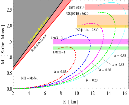
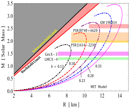
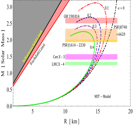
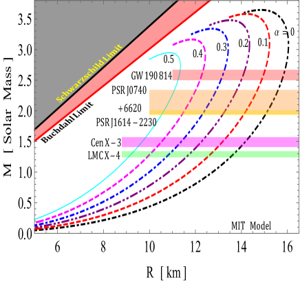
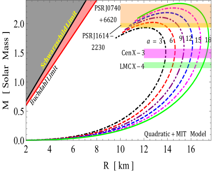
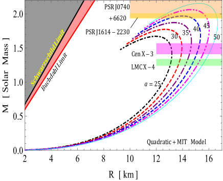
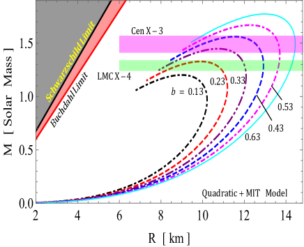
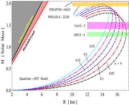
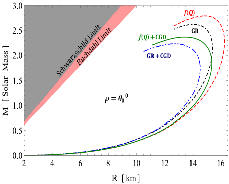
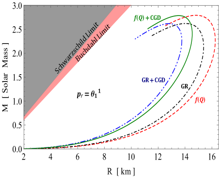
The paper is organized as follows: In Section 2, model equations for f(𝒬)𝑓𝒬f(\mathcal{Q}) gravity with extra source have been provided. In Section 3, extended gravitationally decoupled solution in f(𝒬)𝑓𝒬f(\mathcal{Q}) gravity is studied along with mimicking of the density constraint (i.e., ρ=θ00𝜌subscriptsuperscript𝜃00\rho=\theta^{0}_{0} in 3.1) and mimicking of the pressure constraint (i.e., pr=θ11subscript𝑝𝑟subscriptsuperscript𝜃11p_{r}=\theta^{1}_{1} in 3.2). In Section 4, the matching conditions for the astrophysical system in connection to the exterior spacetime has been elaborated. The physical analysis of completely deformed strange star models and astrophysical implications the problem are done in Section 5 where regular behavior of strange star models are discussed under the cases (i) for solution ρ=θ00𝜌subscriptsuperscript𝜃00\rho=\theta^{0}_{0} (in 5.1.1) and (ii) for solution pr=θ11subscript𝑝𝑟subscriptsuperscript𝜃11p_{r}=\theta^{1}_{1} (in 5.1.2) whereas we have provided the constraining upper limit of maximum mass for strange star via M-R diagrams under the cases (i) Linear EOS with constancy in bag constant, fixed decoupling parameter and varying EOS parameter (in 5.2.1), (ii) linear EOS with constancy in bag constant, fixed EOS parameter and varying decoupling constant (in 5.2.2), (iii) Quadratic EOS with fixed bag constant, fixed decoupling constant with varying quadratic EOS parameter (in 5.2.3), and (iv) Quadratic EOS with fixed bag constant, fixed quadratic EOS parameter with constant versus varying decoupling constant for mimicking of radial pressure, pr=θ11subscript𝑝𝑟subscriptsuperscript𝜃11p_{r}=\theta^{1}_{1}(in 5.2.4). We have discussed the energy exchange between the fluid distributions for T^ijsubscript^𝑇𝑖𝑗\hat{T}_{ij} and θijsubscript𝜃𝑖𝑗\theta_{ij} under the cases (i) for solution ρ=θ00𝜌subscriptsuperscript𝜃00\rho=\theta^{0}_{0} (in 6.0.1) and (ii) for solution pr=θ11subscript𝑝𝑟subscriptsuperscript𝜃11p_{r}=\theta^{1}_{1} (in 6.0.2). In Section 7 the comparative study of model’s arising in GR, GR+CGD, f(𝒬)𝑓𝒬f(\mathcal{Q}) and f(𝒬)𝑓𝒬f(\mathcal{Q})+CGD gravity have been presented while a few concluding remarks are discussed in Section 8.

2 Model equations for f(𝒬)𝑓𝒬f(\mathcal{Q}) gravity with extra source

Let us now have an exposure to the f(𝒬)𝑓𝒬f(\mathcal{Q}) gravity and hence gravitationally decoupled systems in terms of symmetric teleparallel paradigm. The first essential point is that in f(𝒬)𝑓𝒬f(\mathcal{Q}) theory the gravitational interaction is triggered by the non-metric scalar 𝒬𝒬\mathcal{Q}. Therefore, it is always possible that using a second Lagrangian θsubscript𝜃\mathcal{L}_{\theta} for a different source θijsubscript𝜃𝑖𝑗\theta_{ij}, one may express the modified action of f(𝒬)𝑓𝒬f(\mathcal{Q}) gravity for gravitationally decoupled systems in the following way:

𝒮=(12f(𝒬)+λkϱijRϱijk+λkijTijk+m)gd4x𝒮12𝑓𝒬superscriptsubscript𝜆𝑘italic-ϱ𝑖𝑗subscriptsuperscript𝑅𝑘italic-ϱ𝑖𝑗superscriptsubscript𝜆𝑘𝑖𝑗subscriptsuperscript𝑇𝑘𝑖𝑗subscript𝑚𝑔superscript𝑑4𝑥\displaystyle\mathcal{S}=\int{\left(\frac{1}{2}\,f(\mathcal{Q})+\lambda_{k}^{\varrho ij}R^{k}_{\varrho ij}+\lambda_{k}^{ij}T^{k}_{ij}+\mathcal{L}_{m}\right)\sqrt{-g}~{}d^{4}x}
+αθgd4x.𝛼subscript𝜃𝑔superscript𝑑4𝑥\displaystyle\hskip 14.22636pt+\,\alpha\int{\mathcal{L}_{\theta}}\,\sqrt{-g}~{}d^{4}x. (1)

In the above Eq. (1), msubscript𝑚\mathcal{L}_{m} is the matter Lagrangian density, g𝑔g is a determinant of the metric tensor (i.e., g=|gij|𝑔subscript𝑔𝑖𝑗g=|g_{ij}|), α𝛼\alpha represents a decoupling constant, and λkϱijsuperscriptsubscript𝜆𝑘italic-ϱ𝑖𝑗\lambda_{k}^{\varrho ij} defines the Lagrange multipliers. However, within the context of the f(𝒬)𝑓𝒬f(\mathcal{Q}) gravity, the metric tensor gijsubscript𝑔𝑖𝑗g_{ij} and the connection ΓijksubscriptsuperscriptΓ𝑘𝑖𝑗\Gamma^{k}_{\,\,\,ij} are considered individually and the necessary connection for nonmetricity term can be expressed as follows:

Qkij=kgij=igjkΓijlglkΓiklgjl.subscript𝑄𝑘𝑖𝑗subscript𝑘subscript𝑔𝑖𝑗subscript𝑖subscript𝑔𝑗𝑘subscriptsuperscriptΓ𝑙𝑖𝑗subscript𝑔𝑙𝑘subscriptsuperscriptΓ𝑙𝑖𝑘subscript𝑔𝑗𝑙Q_{kij}=\nabla_{{}_{k}}\,g_{ij}=\partial_{i}\,g_{jk}-\Gamma^{l}_{\,\,\,ij}\,g_{lk}-\Gamma^{l}_{\,\,\,ik}\,g_{jl}. (2)

where ksubscript𝑘\nabla_{k} defines the covariant derivative and ΓijksubscriptsuperscriptΓ𝑘𝑖𝑗\Gamma^{k}_{\,\,\,ij} referred to as an affine connection. The final affine connection configuration is defined as

Γijk={ijk}+Kijk+Lijk,\Gamma^{k}_{ij}=\{^{\,\,\,k}_{\,i\,\,j}\}+K^{k}_{\,\,\,ij}+L^{k}_{\,\,ij}, (3)

where {ijk}\{^{\,\,\,k}_{\,i\,\,j}\}, Kijksubscriptsuperscript𝐾𝑘𝑖𝑗K^{k}_{\,\,\,ij} and Lijksubscriptsuperscript𝐿𝑘𝑖𝑗L^{k}_{\,\,ij} define the Levi-Civita connection, contortion tensor and disformation tensor respectively, which are described as:

{ijk}=12gkl(iglj+jglilgij),\displaystyle\{^{\,\,\,k}_{\,i\,\,j}\}=\frac{1}{2}g^{kl}\left(\partial_{i}g_{lj}+\partial_{j}g_{li}-\partial_{l}g_{ij}\right),~{}~{}
Lijk=12QijkQ(ij)k,Kijk=12Tijk+T(ij)k,formulae-sequencesubscriptsuperscript𝐿𝑘𝑖𝑗12subscriptsuperscript𝑄𝑘𝑖𝑗superscriptsubscript𝑄𝑖𝑗𝑘subscriptsuperscript𝐾𝑘𝑖𝑗12subscriptsuperscript𝑇𝑘𝑖𝑗superscriptsubscript𝑇𝑖𝑗𝑘\displaystyle L^{k}_{\,\,\,ij}=\frac{1}{2}Q^{k}_{\,\,\,ij}-Q_{(i\,\,\,\,\,\,j)}^{\,\,\,\,\,\,k},~{}~{}~{}K^{k}_{\,\,\,ij}=\frac{1}{2}T^{k}_{\,\,\,ij}+T_{(i\,\,\,\,\,\,j)}^{\,\,\,\,\,\,k}, (4)

where Tijksubscriptsuperscript𝑇𝑘𝑖𝑗T^{k}_{\,\,i\,j} defines the anti-symmetric part of the affine connection, i.e., Tijk=2Γ[ij]lsubscriptsuperscript𝑇𝑘𝑖𝑗2subscriptsuperscriptΓ𝑙delimited-[]𝑖𝑗T^{k}_{\,\,\,i\,j}=2\Gamma^{l}_{\,\,\,[i\,j]}.

In terms of the nonmetricity tensor, the superpotential is defined as:

Pijk=14[Qijk+2Q(ij)k+QkgijQ~kgijδ(ikQj)].\displaystyle P^{k}_{\,\,\,\,ij}=\frac{1}{4}\left[-Q^{k}_{\,\,\,\,ij}+2Q_{(i\,j)}^{k}+Q^{k}g_{ij}-\tilde{Q}^{k}g_{ij}-\delta^{k}_{(i}Q_{j)}\right].~{}~{}~{} (5)

In particular, there are only two unique traces of the nonmetricity tensor Qkijsubscript𝑄𝑘𝑖𝑗Q_{kij} because of the symmetry of the metric tensor gijsubscript𝑔𝑖𝑗g_{ij}, which can be written as

QkQkii,Q~kQiki.formulae-sequencesubscript𝑄𝑘superscriptsubscript𝑄𝑘𝑖𝑖superscript~𝑄𝑘subscriptsuperscript𝑄𝑘𝑖𝑖\displaystyle Q_{k}\equiv Q_{k\,\,\,~{}i}^{\,\,~{}i},~{}~{}~{}~{}~{}~{}~{}~{}\;\tilde{Q}^{k}\equiv Q^{\,\,\,\,ki}_{i}. (6)

Let us define the nonmetricity scalar in the background of connection as it will be useful in the current analysis and the calculated form of the nonmetricity scalar can be given as

𝒬=14QijkQijk+12QijkQkji+14QiQi12QiQ~i.𝒬14subscript𝑄𝑖𝑗𝑘superscript𝑄𝑖𝑗𝑘12subscript𝑄𝑖𝑗𝑘superscript𝑄𝑘𝑗𝑖14subscript𝑄𝑖superscript𝑄𝑖12subscript𝑄𝑖superscript~𝑄𝑖\mathcal{Q}=-\frac{1}{4}Q_{ijk}Q^{ijk}+\frac{1}{2}Q_{ijk}Q^{kji}+\frac{1}{4}Q_{i}Q^{i}-\frac{1}{2}Q_{i}\tilde{Q}^{i}. (7)

Furthermore, we define Tijsubscript𝑇𝑖𝑗T_{ij} and θijsubscript𝜃𝑖𝑗\theta_{ij} for the current analysis as:

T^ij=2gδ(gm)δgij&θij=2gδ(gθ)δgij.formulae-sequencesubscript^𝑇𝑖𝑗2𝑔𝛿𝑔subscript𝑚𝛿superscript𝑔𝑖𝑗subscript𝜃𝑖𝑗2𝑔𝛿𝑔subscript𝜃𝛿superscript𝑔𝑖𝑗\displaystyle\hat{T}_{ij}=\frac{2}{\sqrt{-g}}\frac{\delta\left(\sqrt{-g}\,\mathcal{L}_{m}\right)}{\delta g^{ij}}\,~{}~{}~{}\&~{}\theta_{ij}=\frac{2}{\sqrt{-g}}\frac{\delta\left(\sqrt{-g}\,\mathcal{L}_{\theta}\right)}{\delta g^{ij}}.~{}~{} (8)

The modified Einstein-Hilbert action within the purview of symmetric teleparallel gravity (i.e. Eq. (1)), can produce the following gravitational field equations by variation of action with respect to the metric tensor gijsuperscript𝑔𝑖𝑗g^{ij}:

2gk(gf𝒬Pijk)+12gijf+f𝒬(PiklQjkl\displaystyle\frac{2}{\sqrt{-g}}\nabla_{k}\left(\sqrt{-g}\,f_{\mathcal{Q}}\,P^{k}_{\,\,\,\,ij}\right)+\frac{1}{2}g_{ij}f+f_{\mathcal{Q}}\big{(}P_{i\,kl}\,Q_{j}^{\,\,\,\,kl}~{}
2QkliPjkl)=Tij,\textwhereTij=(T^ij+αθij),\displaystyle-2\,Q_{kli}\,P^{kl}_{\,\,\,\,\,j}\big{)}=T_{ij},~{}~{}~{}\text{where}~{}~{}T_{ij}=\big{(}\hat{T}_{ij}+\alpha\,\theta_{ij}\big{)},~{}~{}~{}~{} (9)

where f𝒬=f𝒬subscript𝑓𝒬𝑓𝒬f_{\mathcal{Q}}=\frac{\partial f}{\partial\mathcal{Q}}, Tijsubscript𝑇𝑖𝑗T_{ij} is the stress energy-momentum tensor while θijsubscript𝜃𝑖𝑗\theta_{ij} represents the involvement of extra source term.

On the other hand, by varying the action with respect to the connection, one may obtain the following relation:

nλkjin+λkij=gf𝒬Pijk+Hk,ij\displaystyle\nabla_{n}\,\lambda_{k}^{jin}+\lambda_{k}^{ij}=\sqrt{-g}\,f_{\mathcal{Q}}P_{ij}^{k}+H_{k}{}^{ij}, (10)

where HkijH_{k}{}^{ij} represents the density related to hyper-momentum tensor and can be defined as:

Hk=ij12δLmδΓkij.\displaystyle H_{k}{}^{ij}=-\frac{1}{2}\frac{\delta L_{m}}{\delta\Gamma^{k}{}_{ij}}. (11)

Now, by using the antisymmetric property of i𝑖i and j𝑗j in the Lagrangian multiplier coefficients, the Eq. (10) gives the following relation:

ij(gf𝒬Pijk+Hijk)=0.subscript𝑖subscript𝑗𝑔subscript𝑓𝒬subscriptsuperscript𝑃𝑘𝑖𝑗subscriptsuperscript𝐻𝑘𝑖𝑗0\displaystyle\nabla_{i}\nabla_{j}\left(\sqrt{-g}\,f_{\mathcal{Q}}\,P^{k}_{\,\,\,\,ij}+H^{k}_{\,\,\,\,ij}\right)=0.~{}~{} (12)

Additionally, we can retrieve the constraint over the connection, ij(Hijk)=0\bigtriangledown_{i}\bigtriangledown_{j}(H^{k}_{\,\,\,\,ij})=0, according to the Eq. (12) as follows:

ij(gf𝒬Pijk)=0.subscript𝑖subscript𝑗𝑔subscript𝑓𝒬subscriptsuperscript𝑃𝑘𝑖𝑗0\displaystyle\nabla_{i}\nabla_{j}\left(\sqrt{-g}\,f_{\mathcal{Q}}\,P^{k}_{\,\,\,\,ij}\right)=0. (13)

Due to lacking of curvature and torsion, it can be more explicitly parameterized by a number of functions and finally, the affine connection gets the following form:

Γijk=(xkξl)ijξl.subscriptsuperscriptΓ𝑘𝑖𝑗superscript𝑥𝑘superscript𝜉𝑙subscript𝑖subscript𝑗superscript𝜉𝑙\displaystyle\Gamma^{k}_{\,\,\,ij}=\left(\frac{\partial x^{k}}{\partial\xi^{l}}\right)\partial_{i}\partial_{j}\xi^{l}. (14)

Under the current scenario, an invertible relation is ξk=ξk(xi)superscript𝜉𝑘superscript𝜉𝑘superscript𝑥𝑖\xi^{k}=\xi^{k}(x^{i}). As a consequence, there always does exist a possibility of discovering a coordinate system that eliminates the ΓijksubscriptsuperscriptΓ𝑘𝑖𝑗\Gamma^{k}_{\,\,\,ij} connection, i.e. Γijk=0subscriptsuperscriptΓ𝑘𝑖𝑗0\Gamma^{k}_{\,\,\,ij}=0. It is to note that the coincident gauge is the covariant derivative isubscript𝑖\nabla_{i} reduced to the partial one isubscript𝑖\partial_{i}. In any other coordinate system, where this affine relationship does not vanish, the metric development would be altered, resulting in a completely new theory (Dimakis et al., 2022). Therefore, we find a coincident gauge coordinate and nonmetricity by Eq. (2) which can be simplified as

Qkij=kgij.subscript𝑄𝑘𝑖𝑗subscript𝑘subscript𝑔𝑖𝑗\displaystyle Q_{kij}=\partial_{k}\,g_{ij}. (15)

One consequence of the operations stated above is that the metric makes the computation easier, as except for the standard General Relativity, here for the action diffeomorphism invariance no longer does exist. In principle, a covariant formulation of f(𝒬)𝑓𝒬f(\mathcal{Q}) gravity can be used by determining the affine connection in the absence of gravity before choosing the affine connection in Eq. (14). In this paper, we look into the gravitationally decoupled solutions for compact objects under f(𝒬)𝑓𝒬f(\mathcal{Q}) gravity.

For the current analysis, we consider the generic spherically symmetric metric, which is given as:

ds2=eΦ(r)dt2eμ(r)dr2r2(dθ2+sin2θdϕ2).𝑑superscript𝑠2superscript𝑒Φ𝑟𝑑superscript𝑡2superscript𝑒𝜇𝑟𝑑superscript𝑟2superscript𝑟2𝑑superscript𝜃2superscript2𝜃𝑑superscriptitalic-ϕ2ds^{2}=e^{\Phi(r)}dt^{2}-e^{\mu(r)}dr^{2}-r^{2}(d\theta^{2}+\sin^{2}{\theta}\,d\phi^{2}). (16)

In the present study, we consider that the spacetime is filled by the anisotropic matter distribution, then total energy-momentum tensor (Tijsubscript𝑇𝑖𝑗T_{ij}) can be described as:

Tij=ϵuiuj𝒫Kji+Πji,subscript𝑇𝑖𝑗italic-ϵsuperscript𝑢𝑖subscript𝑢𝑗𝒫subscriptsuperscript𝐾𝑖𝑗subscriptsuperscriptΠ𝑖𝑗\displaystyle T_{ij}=\epsilon\,u^{i}\,u_{j}-\mathcal{P}\,K^{i}_{j}+\Pi^{i}_{j}, (17)

where

𝒫=Pr+2P3;Πji=Π(ξiξj+13Kji);formulae-sequence𝒫subscript𝑃𝑟2subscript𝑃perpendicular-to3subscriptsuperscriptΠ𝑖𝑗Πsuperscript𝜉𝑖subscript𝜉𝑗13subscriptsuperscript𝐾𝑖𝑗\displaystyle\mathcal{P}=\frac{P_{r}+2P_{\perp}}{3};~{}~{}~{}\Pi^{i}_{j}=\Pi\big{(}\xi^{i}\xi_{j}+\frac{1}{3}K^{i}_{j}\big{)};~{}~{}
\textwithΠ=PrP;Kji=δjiuiuj,formulae-sequence\text𝑤𝑖𝑡Πsubscript𝑃𝑟subscript𝑃perpendicular-tosubscriptsuperscript𝐾𝑖𝑗subscriptsuperscript𝛿𝑖𝑗superscript𝑢𝑖subscript𝑢𝑗\displaystyle\text{with}~{}~{}\Pi=P_{r}-P_{\perp};~{}~{}~{}K^{i}_{j}=\delta^{i}_{j}-u^{i}u_{j}, (18)

and fluid’s four-velocity vector uisuperscript𝑢𝑖u^{i} and unit space like vector ξisuperscript𝜉𝑖\xi^{i} are given by {i=0,1,2,3}𝑖0123\{i=0,1,2,3\},

ui=(eΦ/2,0,0,0)\textandξi=(0,eμ/2,0,0),superscript𝑢𝑖superscript𝑒Φ2000\text𝑎𝑛𝑑superscript𝜉𝑖0superscript𝑒𝜇200\displaystyle u^{i}=(e^{-\Phi/2},~{}0,~{}0,~{}0)~{}~{}\text{and}~{}~{}\xi^{i}=(0,~{}e^{-\mu/2},~{}0,~{}0),~{}~{} (19)

such that ξiui=0superscript𝜉𝑖subscript𝑢𝑖0\xi^{i}u_{i}=0 and ξiξi=1superscript𝜉𝑖subscript𝜉𝑖1\xi^{i}\xi_{i}=-1. Moreover, ϵitalic-ϵ\epsilon denotes the total energy density while Prsubscript𝑃𝑟P_{r} and Psubscript𝑃perpendicular-toP_{\perp} represent the total radial and tangential pressure, respectively for the gravitationally decoupled system. In this regard, the components of the energy-momentum tensor for gravitationally decoupled system under the spherically symmetric line element (16) are,

T00=ϵ,T11=Pr,T22=T33=P,formulae-sequencesubscriptsuperscript𝑇00italic-ϵformulae-sequencesubscriptsuperscript𝑇11subscript𝑃𝑟subscriptsuperscript𝑇22subscriptsuperscript𝑇33subscript𝑃perpendicular-to\displaystyle T^{0}_{0}=\epsilon,~{}~{}~{}T^{1}_{1}=-P_{r},~{}~{}~{}~{}T^{2}_{2}=T^{3}_{3}=-P_{\perp}, (20)

For the metric Equation (16), we can calculate the nonmetricity scalar as follows:

𝒬=2eμ(r)[1+rΦ(r)]r2,𝒬2superscript𝑒𝜇𝑟delimited-[]1𝑟superscriptΦ𝑟superscript𝑟2\mathcal{Q}=-\frac{2e^{-\mu(r)}\left[1+r\,\Phi^{\prime}(r)\right]}{r^{2}}, (21)

where the notation denotes the derivative over the radial coordinate r𝑟r only.

In the above expression, 𝒬𝒬\mathcal{Q} is based on the zero affine connections which can be absorbed via the equations of motion (2) for the anisotropic fluid (18) as follows:

ϵ=f(𝒬)2+f𝒬(𝒬)[𝒬+1r2+eμr(Φ+μ)],italic-ϵ𝑓𝒬2subscript𝑓𝒬𝒬delimited-[]𝒬1superscript𝑟2superscript𝑒𝜇𝑟superscriptΦsuperscript𝜇\displaystyle\epsilon=-\frac{f(\mathcal{Q})}{2}+f_{\mathcal{Q}}(\mathcal{Q})\Big{[}\mathcal{Q}+\frac{1}{r^{2}}+\frac{e^{-\mu}}{r}(\Phi^{\prime}+\mu^{\prime})\Big{]}, (22)
Pr=f(𝒬)2f𝒬(𝒬)[𝒬+1r2],subscript𝑃𝑟𝑓𝒬2subscript𝑓𝒬𝒬delimited-[]𝒬1superscript𝑟2\displaystyle P_{r}=\frac{f(\mathcal{Q})}{2}-f_{\mathcal{Q}}(\mathcal{Q})\Big{[}\mathcal{Q}+\frac{1}{r^{2}}\Big{]}, (23)
P=f(𝒬)2f𝒬(𝒬)[𝒬2eμ{Φ′′2+(Φ4+12r)\displaystyle P_{\perp}=\frac{f(\mathcal{Q})}{2}-f_{\mathcal{Q}}(\mathcal{Q})\Big{[}\frac{\mathcal{Q}}{2}-e^{-\mu}\Big{\{}\frac{\Phi^{\prime\prime}}{2}+\Big{(}\frac{\Phi^{\prime}}{4}+\frac{1}{2r}\Big{)}~{}
×(Φμ)}],\displaystyle\hskip 4.26773pt\times(\Phi^{\prime}-\mu^{\prime})\Big{\}}\Big{]},~{}~{}~{}~{}~{}~{}~{}~{} (24)
0=\textcotθ2𝒬f𝒬𝒬(𝒬),0\text𝑐𝑜𝑡𝜃2superscript𝒬subscript𝑓𝒬𝒬𝒬\displaystyle 0=\frac{\text{cot}\,\theta}{2}\,\mathcal{Q}^{\prime}\,f_{\mathcal{Q}\mathcal{\mathcal{Q}}}(\mathcal{Q}), (25)

where f𝒬(𝒬)=f(𝒬)𝒬subscript𝑓𝒬𝒬𝑓𝒬𝒬f_{\mathcal{Q}}(\mathcal{Q})=\frac{\partial f(\mathcal{Q})}{\partial\mathcal{\mathcal{Q}}} and f𝒬𝒬(Q)=2f(𝒬)𝒬2subscript𝑓𝒬𝒬𝑄superscript2𝑓𝒬superscript𝒬2f_{\mathcal{Q}\mathcal{Q}}(Q)=\frac{\partial^{2}f(\mathcal{Q})}{\partial\mathcal{Q}^{2}}.

It is to be noted that the nonzero off-diagonal metric components derived from the specific gauge choice for the field equations in the context of f(T)𝑓𝑇f(T) theory put some constraints on the functional form of f(T)𝑓𝑇f(T) (Ferraro & Fiorini, 2011). As a consequence, it imposes restrictions on the functional form of f(𝒬)𝑓𝒬f(\mathcal{Q}) theory. In this connection, Wang et al. (2022) derived the possible functional forms for f(𝒬)𝑓𝒬f(\mathcal{Q}) gravity in the framework of the static and spherically symmetric spacetime by taking an anisotropic matter distribution. More specifically, they have shown that the exact Schwarzschild solution can exist only when f𝒬𝒬(𝒬)=0subscript𝑓𝒬𝒬𝒬0f_{\mathcal{Q}\mathcal{Q}}(\mathcal{Q})=0, while the solution obtained by taking nonmetricity scalar 𝒬=0superscript𝒬0\mathcal{Q}^{\prime}=0 or 𝒬=𝒬0𝒬subscript𝒬0\mathcal{Q}=\mathcal{Q}_{0}, where Q0subscript𝑄0Q_{0} is constant, shows the deviation from the exact Schwarzschild solution (The detailed analysis of above derivation is given in section 4). Therefore, in order to solve the system of field equations in f(𝒬)𝑓𝒬f(\mathcal{Q})-gravity theory for obtaining self-gravitating compact objects, we derive the functional form of f(𝒬)𝑓𝒬f(\mathcal{Q}) by taking only f𝒬𝒬subscript𝑓𝒬𝒬f_{\mathcal{Q}\mathcal{Q}} to be zero as

f𝒬𝒬(𝒬)=0f𝒬(𝒬)=β1f(𝒬)=β1𝒬+β2,subscript𝑓𝒬𝒬𝒬0subscript𝑓𝒬𝒬subscript𝛽1𝑓𝒬subscript𝛽1𝒬subscript𝛽2\displaystyle f_{\mathcal{Q}\mathcal{Q}}(\mathcal{Q})=0~{}\Rightarrow~{}f_{\mathcal{Q}}(\mathcal{Q})=\beta_{1}~{}\Rightarrow~{}f(\mathcal{Q})=\beta_{1}\,\mathcal{Q}+\beta_{2},~{}~{}~{}~{} (26)

where β1subscript𝛽1\beta_{1} and β2subscript𝛽2\beta_{2} are constants.

At this juncture, we would like to mention that the compatibility of static spherically symmetric spacetime with the coincident gauge, if one assumes the affine connection to be zero and f(𝒬)𝑓𝒬f(\mathcal{Q})-gravity theory has vacuum solutions (i.e. Tij=0subscript𝑇𝑖𝑗0T_{ij}=0), then the off-diagonal component can be given by

\textcotθ2𝒬f𝒬𝒬=0,\text𝑐𝑜𝑡𝜃2superscript𝒬subscript𝑓𝒬𝒬0\displaystyle\frac{\text{cot}\,\theta}{2}\,\mathcal{Q}^{\prime}\,f_{\mathcal{Q}\mathcal{Q}}=0, (27)

where 𝒬𝒬\mathcal{Q} has been provided by Eq. (21).

As a consequence of the above Eq. 26 it can be explored that f(𝒬)𝑓𝒬f(\mathcal{Q}) to be linear, the equations of motion automatically turn into f𝒬𝒬=0subscript𝑓𝒬𝒬0f_{\mathcal{Q}\mathcal{Q}}=0 (Zhao, 2022). This aspect is very essential as the non-linear function of 𝒬𝒬\mathcal{Q} would gives rise to inconsistent equations of motion. This implies that we need for a more generalized form of the spherically symmetric metric related to a fixed coincident gauge (Zhao, 2022). Therefore, in the present study to make the spherically symmetric coordinate system compatible one with affine connection Γijk=0subscriptsuperscriptΓ𝑘𝑖𝑗0\Gamma^{k}_{ij}=0, we have opted for the linear functional form by considering f𝒬𝒬=0subscript𝑓𝒬𝒬0f_{\mathcal{Q}\mathcal{Q}}=0 to derive the equations of motion.

Now inserting Eqs. (21) and (26) into Eqs. (22)–(24), the equations of motion can be obtained as follows:

ϵ=12r2[2β1+2eμβ1(rμ1)r2β2],italic-ϵ12superscript𝑟2delimited-[]2subscript𝛽12superscript𝑒𝜇subscript𝛽1𝑟superscript𝜇1superscript𝑟2subscript𝛽2\displaystyle\epsilon=\frac{1}{2\,r^{2}}\Big{[}2\,\beta_{1}+2\,e^{-\mu}\,\beta_{1}\left(r\,\mu^{\prime}-1\right)-r^{2}\,\beta_{2}\Big{]}, (28)
Pr=12r2[2β1+2eμβ1(rΦ+1)+r2β2],subscript𝑃𝑟12superscript𝑟2delimited-[]2subscript𝛽12superscript𝑒𝜇subscript𝛽1𝑟superscriptΦ1superscript𝑟2subscript𝛽2\displaystyle P_{r}=\frac{1}{2\,r^{2}}\Big{[}-2\,\beta_{1}+2\,e^{-\mu}\,\beta_{1}\left(r\,\Phi^{\prime}+1\right)+r^{2}\,\beta_{2}\Big{]}, (29)
P=eμ4r[2eμrβ2+β1(2+rΦ)(Φμ)\displaystyle P_{\perp}=\frac{e^{-\mu}}{4\,r}\Big{[}2\,e^{\mu}\,r\,\beta_{2}+\beta_{1}\,\left(2+r\Phi^{\prime}\,\right)\left(\Phi^{\prime}-\mu^{\prime}\right)
+2rβ1Φ′′],\displaystyle\hskip 19.91684pt+2\,r\,\beta_{1}\,\Phi^{\prime\prime}\Big{]},~{}~{}~{}~{} (30)

The vanishing of the covariant derivative of the effective energy-momentum tensor is iTji=0subscript𝑖subscriptsuperscript𝑇𝑖𝑗0\bigtriangledown_{i}T^{i}_{j}=0, provides

H2(ϵ+Pr)(Pr)+2r(PPr)=0.superscript𝐻2italic-ϵsubscript𝑃𝑟superscriptsubscript𝑃𝑟2𝑟subscript𝑃perpendicular-tosubscript𝑃𝑟0\displaystyle-\frac{H^{\prime}}{2}(\epsilon+P_{r})-(P_{r})^{\prime}+\frac{2}{r}(P_{\perp}-P_{r})=0.~{}~{}~{} (31)

It is to be noted that the above Eq. (31) is nothing but the usual Tolman-Oppenheimer-Volkoff (TOV) equation (Tolman, 1939; Oppenheimer & Volkoff, 1939), with f(𝒬)=β1𝒬+β2𝑓𝒬subscript𝛽1𝒬subscript𝛽2f(\mathcal{Q})=\beta_{1}\mathcal{Q}+\beta_{2}. Therefore, in connection to the proposed compact stellar model we would like to employ gravitational decoupling under the CGD approach to get solution to the system of Eqs. (28)–(30). For this specific purpose, the gravitational potentials Φ(r)Φ𝑟\Phi(r) and μ(r)𝜇𝑟\mu(r) are essential to modify as follows:

Φ(r)H(r)+αη(r)Φ𝑟𝐻𝑟𝛼𝜂𝑟\displaystyle\Phi(r)\longrightarrow H(r)+\alpha\,\eta(r)~{} (32)
eμ(r)W(r)+αΨ(r),superscript𝑒𝜇𝑟𝑊𝑟𝛼Ψ𝑟\displaystyle e^{-\mu(r)}\longrightarrow W(r)+\alpha\,\Psi(r),~{}~{}~{}~{} (33)

where Φ(r)Φ𝑟\Phi(r) and μ(r)𝜇𝑟\mu(r) are two arbitrary deformation functions via the decoupling constant β𝛽\beta whereas in the resultant parts η(r)𝜂𝑟\eta(r) and Ψ(r)Ψ𝑟\Psi(r) are the geometric deformation functions for the temporal and radial metric components, respectively.

In the above Eqs. (32) and (33), for α=0𝛼0\alpha=0, the standard f(𝒬)𝑓𝒬f(\mathcal{Q}) gravity theory can be easily recovered. Essentially in the present work to continue, we must consider the non-zero value for both the deformation functions, i.e., η(r)0𝜂𝑟0\eta(r)\neq 0 and Ψ(r)0Ψ𝑟0\Psi(r)\neq 0. The above transformations (32) and (33) can easily divide the decoupled system, viz. (28)–(30), into two subsystems which are as follows: (i) the first system reflects the field equation in f(𝒬)𝑓𝒬f(\mathcal{Q}) gravity under Tijsubscript𝑇𝑖𝑗T_{i\,j} and (ii) the second system represents the additional source θijsubscript𝜃𝑖𝑗\theta_{i\,j}. To include all these systems, we need to specify the form of energy-momentum tensor Tijsubscript𝑇𝑖𝑗T_{i\,j} in the following form:

T^ji=ρχiχj𝒫𝒬hji+Π^ji,subscriptsuperscript^𝑇𝑖𝑗𝜌superscript𝜒𝑖subscript𝜒𝑗subscript𝒫𝒬subscriptsuperscript𝑖𝑗subscriptsuperscript^Π𝑖𝑗\displaystyle\hat{T}^{i}_{j}=\rho\,\chi^{i}\,\chi_{j}-\mathcal{P}_{\mathcal{Q}}\,h^{i}_{j}+\hat{\Pi}^{i}_{j}~{}, (34)

where

𝒫𝒬=pr+2p3;Π^ji=Π𝒬(ζiζj+13hji);formulae-sequencesubscript𝒫𝒬subscript𝑝𝑟2subscript𝑝perpendicular-to3subscriptsuperscript^Π𝑖𝑗subscriptΠ𝒬superscript𝜁𝑖subscript𝜁𝑗13subscriptsuperscript𝑖𝑗\displaystyle\mathcal{P}_{\mathcal{Q}}=\frac{p_{r}+2p_{\perp}}{3}~{};~{}~{}~{}\hat{\Pi}^{i}_{j}=\Pi_{\mathcal{Q}}\big{(}\zeta^{i}\zeta_{j}+\frac{1}{3}h^{i}_{j}\big{)}~{};
\textwithΠ𝒬=prpt;hji=δjiχiχj,formulae-sequence\text𝑤𝑖𝑡subscriptΠ𝒬subscript𝑝𝑟subscript𝑝𝑡subscriptsuperscript𝑖𝑗subscriptsuperscript𝛿𝑖𝑗superscript𝜒𝑖subscript𝜒𝑗\displaystyle~{}~{}\text{with}~{}~{}~{}\Pi_{\mathcal{Q}}=p_{r}-p_{t}~{};~{}~{}h^{i}_{j}=\delta^{i}_{j}-\chi^{i}\chi_{j}~{}, (35)

and χisuperscript𝜒𝑖\chi^{i} (fluid’s four-velocity vector) and ζisuperscript𝜁𝑖\zeta^{i} (unit space like vector) are given by,

χi=(eH/2,0,0,0)\textandζi=(0,W,0,0),superscript𝜒𝑖superscript𝑒𝐻2000\text𝑎𝑛𝑑superscript𝜁𝑖0𝑊00\displaystyle\chi^{i}=(e^{-H/2},~{}0,~{}0,~{}0)~{}~{}\text{and}~{}~{}\zeta^{i}=(0,~{}\sqrt{W},~{}0,~{}0), (36)

such that ξiζi=0superscript𝜉𝑖subscript𝜁𝑖0\xi^{i}\zeta_{i}=0 and ζiζi=1superscript𝜁𝑖subscript𝜁𝑖1\zeta^{i}\zeta_{i}=-1. The ϵitalic-ϵ\epsilon, Prsubscript𝑃𝑟P_{r} and Psubscript𝑃perpendicular-toP_{\perp} can be written as,

ϵ=ρ+αθ00,Pr=prαθ11,P=ptαθ22,formulae-sequenceitalic-ϵ𝜌𝛼subscriptsuperscript𝜃00formulae-sequencesubscript𝑃𝑟subscript𝑝𝑟𝛼subscriptsuperscript𝜃11subscript𝑃perpendicular-tosubscript𝑝𝑡𝛼subscriptsuperscript𝜃22\displaystyle\epsilon=\rho+\alpha\,\theta^{0}_{0},~{}~{}P_{r}=p_{{}_{r}}-\alpha\,\theta^{1}_{1},~{}~{}P_{\perp}=p_{{}_{t}}-\alpha\,\theta^{2}_{2},~{}~{}~{}~{} (37)

and the corresponding total anisotropy,

Δ=PPr=Δ𝒬+Δθ,Δsubscript𝑃perpendicular-tosubscript𝑃𝑟subscriptΔ𝒬subscriptΔ𝜃\displaystyle\Delta=P_{\perp}-P_{r}=\Delta_{\mathcal{Q}}+\Delta_{\theta}, (38)

where Δ𝒬=ptpr\textandΔθ=α(θ11θ22).subscriptΔ𝒬subscript𝑝𝑡subscript𝑝𝑟\text𝑎𝑛𝑑subscriptΔ𝜃𝛼subscriptsuperscript𝜃11subscriptsuperscript𝜃22~{}\Delta_{\mathcal{Q}}=p_{{}_{t}}-p_{{}_{r}}~{}~{}\text{and}~{}~{}\Delta_{\theta}=\alpha(\theta^{1}_{1}-\theta^{2}_{2}).

One may note that in the present anisotropic compact stellar system there are two types of anisotropies, viz. Tijsubscript𝑇𝑖𝑗T_{i\,j} and θijsubscript𝜃𝑖𝑗\theta_{i\,j}. Another anisotropy ΔθsubscriptΔ𝜃\Delta_{\theta} comes in the picture due to gravitational decoupling which has a definite role in the transformation processes.

By putting Eqs. (32) and (33) in the system (28)–(30), the set of equations of motion dependent on the gravitational potentials (H(r)𝐻𝑟H(r) and W(r)𝑊𝑟W(r), or when α=0𝛼0\alpha=0), are produced:

ρ=β1(1W)r2Wβ1rβ22,𝜌subscript𝛽11𝑊superscript𝑟2superscript𝑊subscript𝛽1𝑟subscript𝛽22\displaystyle\rho=\frac{\beta_{1}(1-W)}{r^{2}}-\frac{W^{\prime}\beta_{1}}{r}-\frac{\beta_{2}}{2}, (39)
pr=β1(W1)r2+HWβ1r+β22,subscript𝑝𝑟subscript𝛽1𝑊1superscript𝑟2superscript𝐻𝑊subscript𝛽1𝑟subscript𝛽22\displaystyle p_{{}_{r}}=\frac{\beta_{1}(W-1)}{r^{2}}+\frac{H^{\prime}W\beta_{1}}{r}+\frac{\beta_{2}}{2}, (40)
pt=β1(WH+2H′′W+H2W)4+β1(W+HW)2rsubscript𝑝𝑡subscript𝛽1superscript𝑊superscript𝐻2superscript𝐻′′𝑊superscript𝐻2𝑊4subscript𝛽1superscript𝑊superscript𝐻𝑊2𝑟\displaystyle p_{{}_{t}}=\frac{\beta_{1}(W^{\prime}H^{\prime}+2H^{\prime\prime}W+H^{\prime 2}W)}{4}+\frac{\beta_{1}\,(W^{\prime}+H^{\prime}W)}{2r}
+β22,subscript𝛽22\displaystyle\hskip 14.22636pt+\frac{\beta_{2}}{2},~{}~{}~{} (41)

and according to the TOV Eq. (31),

H2(ρ+pr)(pr)+2r(ptpr)=0.superscript𝐻2𝜌subscript𝑝𝑟superscriptsubscript𝑝𝑟2𝑟subscript𝑝𝑡subscript𝑝𝑟0\displaystyle-\frac{H^{\prime}}{2}(\rho+p_{{}_{r}})-(p_{{}_{r}})^{\prime}+\frac{2}{r}(p_{{}_{t}}-p_{{}_{r}})=0.~{}~{} (42)

Consequently, the spacetime that follows can provide the corresponding solution:

ds2=eH(r)dt2+dr2W(r)+r2dθ2+r2\textsin2θdϕ2.𝑑superscript𝑠2superscript𝑒𝐻𝑟𝑑superscript𝑡2𝑑superscript𝑟2𝑊𝑟superscript𝑟2𝑑superscript𝜃2superscript𝑟2\text𝑠𝑖superscript𝑛2𝜃𝑑superscriptitalic-ϕ2ds^{2}=-e^{H(r)}dt^{2}+\frac{dr^{2}}{W(r)}+r^{2}d\theta^{2}+r^{2}\text{sin}^{2}\theta d\phi^{2}. (43)

Moreover, the system of field equations for θ𝜃\theta-sector is derived by turning on α𝛼\alpha as,

θ00=β1(Ψr2+Ψr),subscriptsuperscript𝜃00subscript𝛽1Ψsuperscript𝑟2superscriptΨ𝑟\displaystyle\theta^{0}_{0}=-\beta_{1}\Big{(}\frac{\Psi}{r^{2}}+\frac{\Psi^{\prime}}{r}\Big{)}, (44)
θ11=β1[Ψr2+(ΦΨ+Wη)r],subscriptsuperscript𝜃11subscript𝛽1delimited-[]Ψsuperscript𝑟2superscriptΦΨ𝑊superscript𝜂𝑟\displaystyle\theta^{1}_{1}=-\beta_{1}\Big{[}\frac{\Psi}{r^{2}}+\frac{(\Phi^{\prime}\Psi+W\,\eta^{\prime})}{r}\Big{]}, (45)
θ22=β1[(ΨΦ+2Φ′′Ψ+Φ2Ψ+Wη)4+(Ψ+ΦΨ)2r]subscriptsuperscript𝜃22subscript𝛽1delimited-[]superscriptΨsuperscriptΦ2superscriptΦ′′ΨsuperscriptΦ2Ψsuperscript𝑊superscript𝜂4superscriptΨsuperscriptΦΨ2𝑟\displaystyle\theta^{2}_{2}=-\beta_{1}\Big{[}\frac{(\Psi^{\prime}\Phi^{\prime}+2\Phi^{\prime\prime}\Psi+\Phi^{\prime 2}\Psi+W^{\prime}\,\eta^{\prime})}{4}+\frac{(\Psi^{\prime}+\Phi^{\prime}\Psi)}{2r}\Big{]}
β1[W4(2η′′+αη 2+2ηr+2Hη)],subscript𝛽1delimited-[]𝑊42superscript𝜂′′𝛼superscript𝜂22superscript𝜂𝑟2superscript𝐻superscript𝜂\displaystyle\hskip 14.22636pt-\beta_{1}\Big{[}\frac{W}{4}\,\big{(}2\,\eta^{\prime\prime}+\alpha\,\eta^{{\prime}\,2}+\frac{2\,\eta^{\prime}}{r}+2\,H^{\prime}\,\eta^{\prime}\big{)}\Big{]},~{}~{}~{}~{}~{}~{} (46)

and the associated conservation is

Φ2(θ00θ11)+(θ11)+2r(θ11θ22)=η2(pr+ρ).superscriptΦ2subscriptsuperscript𝜃00subscriptsuperscript𝜃11superscriptsubscriptsuperscript𝜃112𝑟subscriptsuperscript𝜃11subscriptsuperscript𝜃22superscript𝜂2subscript𝑝𝑟𝜌\displaystyle-\frac{\Phi^{\prime}}{2}(\theta^{0}_{0}-\theta^{1}_{1})+(\theta^{1}_{1})^{\prime}+\frac{2}{r}(\theta^{1}_{1}-\theta^{2}_{2})=\frac{\eta^{\prime}}{2}\,({p_{r}}+{\rho}). (47)

However, the mass function for both systems is given by

m𝒬=120rρ(x)x2𝑑x\textan𝑑mθ=120rθ00(x)x2𝑑x,subscript𝑚𝒬12subscriptsuperscript𝑟0𝜌𝑥superscript𝑥2differential-d𝑥\text𝑎𝑛differential-dsubscript𝑚𝜃12superscriptsubscript0𝑟subscriptsuperscript𝜃00𝑥superscript𝑥2differential-d𝑥\displaystyle m_{\mathcal{Q}}=\frac{1}{2}\int^{r}_{0}\rho(x)\,x^{2}dx~{}~{}\text{and}~{}~{}m_{\theta}=\frac{1}{2}\,\int_{0}^{r}\theta^{0}_{0}(x)\,x^{2}dx,~{}~{}~{} (48)

where the relevant mass functions for the sources Tijsubscript𝑇𝑖𝑗T_{ij} and θijsubscript𝜃𝑖𝑗\theta_{ij} are m𝒬(r)subscript𝑚𝒬𝑟m_{\mathcal{Q}}(r) and mθ(r)subscript𝑚𝜃𝑟m_{\theta}(r), respectively. Then, in the context of f(𝒬)𝑓𝒬f(\mathcal{Q}) gravity, the interior mass function of the minimally deformed space-time (16) may be expressed as

m~(r)=m𝒬(r)β1α2rΨ(r).~𝑚𝑟subscript𝑚𝒬𝑟subscript𝛽1𝛼2𝑟Ψ𝑟\displaystyle\tilde{m}(r)=m_{\mathcal{Q}}(r)-\frac{\beta_{1}\,\alpha}{2}\,r\,\Psi(r). (49)

Therefore, from all the previous steps towards the generation of the mass functions, the need as well as advantage of CGD-decoupling becomes very straightforward as such it can be pointed out that one can extend any known solutions associated with the action 𝒮𝒬subscript𝒮𝒬\mathcal{S}_{\mathcal{Q}} with solution {Tij,W,H}subscript𝑇𝑖𝑗𝑊𝐻\{T_{ij},W,H\} of the system (e.g. Eqs. (39)–(41)) into the domain beyond of f(𝒬)𝑓𝒬f(\mathcal{Q}) gravity theory associated with the action 𝒮𝒮\mathcal{S}. It is to be noted that in the process equation of motion are displayed in Eqs. (28)–(30) and the unconventional gravitational system of equations are Eqs. (44)–(48) to determine {θij\{\theta_{ij}, ΨΨ\Psi, η}\eta\}.

Let us now generate the θ𝜃\theta-version of any {Tij,W,H}subscript𝑇𝑖𝑗𝑊𝐻\{T_{ij},W,H\}-solution as

{Tij,H(r),W(r)}{Tij\texttot,Φ(r),μ(r)}.subscript𝑇𝑖𝑗𝐻𝑟𝑊𝑟subscriptsuperscript𝑇\text𝑡𝑜𝑡𝑖𝑗Φ𝑟𝜇𝑟\displaystyle\{T_{ij},~{}H(r),~{}W(r)\}\Longrightarrow\{T^{\text{tot}}_{ij},~{}\Phi(r),~{}\mu(r)\}. (50)

which describes a definite way to investigate the results that is beyond the symmetric teleparallel gravity.

3 Extended gravitationally decoupled solution in f(𝒬)𝑓𝒬f(\mathcal{Q}) gravity

In this Section, we will solve both systems of equations (36)–(39) and (41)–(44) related to the sources Tμνsubscript𝑇𝜇𝜈{T}_{\mu\nu} and θμνsubscript𝜃𝜇𝜈\theta_{\mu\nu}. It is mentioned that the energy-momentum tensor Tijsubscript𝑇𝑖𝑗{T}_{ij} describes an anisotropic fluid matter distribution, therefore, the θijsubscript𝜃𝑖𝑗\theta_{ij} may enhance the total anisotropy of the system which helps in preventing the gravitational collapse of the system. Furthermore, if we look at the second system, it shows clearly that the solution of the second system depends on the first system. Then it is mandatory to solve the first system initially. For solving the first system (36)–(39) in f(𝒬)𝑓𝒬f(\mathcal{Q})-gravity, we use a generalized polytropic equation of state (EOS) of the form,

prsubscript𝑝𝑟\displaystyle p_{r} =\displaystyle= aρ1+1/n+bρ+c,𝑎superscript𝜌11𝑛𝑏𝜌𝑐\displaystyle a\,\rho^{1+1/n}+b\rho+c, (51)

where a,b𝑎𝑏a,~{}b and c𝑐c are constant parameters with proper dimensions and n𝑛n denotes a polytropic index.

Let us trace back the generic history of the polytropic equation of state pr=aρ1+1nsubscript𝑝𝑟𝑎superscript𝜌11𝑛p_{r}=a\rho^{1+\frac{1}{n}} which has been extensively used to analyse the physical attributes of the compact stellar objects in the context of various requirements (Abramowicz, 1983; Cosenza et al., 1981; Herrera & Barreto, 2004; Herrera et al., 2004; Herrera & Barreto, 2013; Herrera et al., 2014, 2016; Bekenstein, 1960; Takisa & Maharaj, 2013; Azam & Mardan, 2017). In connection to cosmological scenario Chavanis (2014a) first tried to generalize the polytropic EOS in the form pr=γρ1+1n+βρsubscript𝑝𝑟𝛾superscript𝜌11𝑛𝛽𝜌p_{r}=\gamma\rho^{1+\frac{1}{n}}+\beta\rho. In the context of the late universe Chavanis (2014b) further studied the issues by considering negative indices which was immediately received attention to the study of quantum fluctuations and constant-density cosmology (Freitas & Goncalves, 2014). But, this EOS is mostly applicable for a stellar system with vanishing pressure when the density goes to zero. Therefore, for the self-bound compact objects, a further modified EOS pr=γρ1+1n+βρ+χsubscript𝑝𝑟𝛾superscript𝜌11𝑛𝛽𝜌𝜒p_{r}=\gamma\rho^{1+\frac{1}{n}}+\beta\rho+\chi was extensively considered by several investigators (Azam et al., 2015, 2016; Azam & Mardan, 2017; Naeem et al., 2021).

It is interesting to note that the polytropic EOS (51) may represent a MIT bag EOS for the specifications: a=0,b=14formulae-sequence𝑎0𝑏14a=0,~{}b=\frac{1}{4} and c=43g𝑐43subscript𝑔c=-\frac{4}{3}\mathcal{B}_{g}, where gsubscript𝑔\mathcal{B}_{g} is a bag constant. Due to highly non-linearity of the field equations, as a simple case we assume the value for the polytropic index as n=1𝑛1n=1. In this context one may note that the contribution for quadratic term (i.e. aρ2𝑎superscript𝜌2a\rho^{2}) appears in the EOS to express the neutron liquid in Bose-Einstein condensate form whereas the linear terms (i.e. bρ+c𝑏𝜌𝑐b\rho+c) come from the free quarks model of the MIT bag model, with b=1/3𝑏13b=1/3 and c=4g/3𝑐4subscript𝑔3c=-4\mathcal{B}_{g}/3.

In addition to the above studies, there are various works employing more realistic EOSs. Analytical representations of more realistic EOS based on parameters arising in nuclear physics such as the FPS EOS due to Pandharipande & Ravenhall (Pandharipande & Ravenhall, 1989), SLy EOS of Douchin & Haensel (Douchin & Haensel, 2001) and the unified EOSs BSK19, BSk20 and BSk21 (Potekhin et al., 2013), amongst others have been previously employed using numerical techniques to generate neutron star models. The quadratic EOS can be viewed as a truncation of these more realistic EOSs. The models derived using the quadratic EOS can be used as first approximation to test more complicated numerical codes. Furthermore, Haensel and Potekhin (Haensel & Potekhin, 2004) pointed out that unified EOSs (presented in the form of tables) introduce ambiguities in the calculations of various parameters in neutron star modeling. These pathologies arise in the interpolation between the tabulated points as well as the calculation of derivatives regarding thermodynamical quantities. They further highlight the point that analytical EOSs ensure that shortcomings are circumnavigated and allow for high-precision neutron star modeling.

Now, by using Eqs. (39) and (40) in Eq. (51), one can find the differential equation

4β1r2(aβ2aβ1W2aβ2W+bWb+W1)+4β1r34subscript𝛽1superscript𝑟2𝑎subscript𝛽2𝑎subscript𝛽1superscript𝑊2𝑎subscript𝛽2𝑊𝑏𝑊𝑏𝑊14subscript𝛽1superscript𝑟3\displaystyle 4\beta_{1}r^{2}\left(a\beta_{2}-a\beta_{1}W^{\prime 2}-a\beta_{2}W+bW-b+W-1\right)+4\beta_{1}r^{3}
×(aβ2W+bW+HW)+β2r4(aβ2+2b+2)8aβ12absent𝑎subscript𝛽2superscript𝑊𝑏superscript𝑊superscript𝐻𝑊subscript𝛽2superscript𝑟4𝑎subscript𝛽22𝑏28𝑎superscriptsubscript𝛽12\displaystyle\times(-a\beta_{2}W^{\prime}+bW^{\prime}+H^{\prime}W)+\beta_{2}r^{4}(-a\beta_{2}+2b+2)-8a\beta_{1}^{2}
×W(W1)r4aβ12(W1)24cr4=0.\displaystyle\times W^{\prime}(W-1)r-4a\beta_{1}^{2}(W-1)^{2}-4cr^{4}=0. (52)

The Eq.(52) leads directly to,

H(r)=G(W,W,r¯)𝑑r¯𝐻𝑟𝐺𝑊superscript𝑊¯𝑟differential-d¯𝑟H(r)=\int{G(W,W^{\prime},{\bar{r})\,{d\bar{r}}}} (53)

where

G(W,W,r)𝐺𝑊superscript𝑊𝑟\displaystyle G(W,W^{\prime},r) =\displaystyle= 14β1r3W[4β1r2(aβ2aβ1W2aβ2W\displaystyle\frac{1}{4\beta_{1}r^{3}W}\Big{[}-4\beta_{1}r^{2}\Big{(}a\beta_{2}-a\beta_{1}W^{\prime 2}-a\beta_{2}W
+bWb+W1)4β1r3(aβ2W+bW)\displaystyle+bW-b+W-1\Big{)}-4\beta_{1}r^{3}(-a\beta_{2}W^{\prime}+bW^{\prime})
β2r4(aβ2+2b+2)+8aβ12W(W1)rsubscript𝛽2superscript𝑟4𝑎subscript𝛽22𝑏28𝑎superscriptsubscript𝛽12superscript𝑊𝑊1𝑟\displaystyle-\beta_{2}r^{4}(-a\beta_{2}+2b+2)+8a\beta_{1}^{2}W^{\prime}(W-1)r
4aβ12(W1)2+4cr4].\displaystyle-4a\beta_{1}^{2}(W-1)^{2}+4cr^{4}\Big{]}.

The above differential equation (53) depends on one undermined unknown W𝑊W. Therefore, we assume a well-known ansatz for W𝑊W for the Buchdahl model to solve the above differential equation,

W(r)=1+Lr21+Nr2,𝑊𝑟1𝐿superscript𝑟21𝑁superscript𝑟2\displaystyle W(r)=\frac{1+Lr^{2}}{1+Nr^{2}}, (54)

where L𝐿L and N𝑁N are constants with dimensions \textlength2\text𝑙𝑒𝑛𝑔𝑡superscript2\text{length}^{-2} and \textlength4\text𝑙𝑒𝑛𝑔𝑡superscript4\text{length}^{-4}, respectively. Now plugging of Eq. (54) into Eq. (53) and integrate, we obtain the solution for H(r)𝐻𝑟H(r) of the form,

H(r)=18[1β1L2(LN)(log(Lr2+1){4β1L3(3aβ26aβ1\displaystyle H(r)=\frac{1}{8}\Bigg{[}\frac{1}{\beta_{1}L^{2}(L-N)}\Big{(}\log\left(Lr^{2}+1\right)\Big{\{}4\beta_{1}L^{3}(3a\beta_{2}-6a\beta_{1}
×N3b1)+L2[β2(aβ22b2)+8β1N(12aβ2+2b)\displaystyle\hskip 5.69046pt\times N-3b-1)+L^{2}[\beta_{2}(a\beta_{2}-2b-2)+8\beta_{1}N(1-2a\beta_{2}+2b)
+4aβ12N2]2LN(β2(aβ22b2)+2β1N(aβ2+b+1))\displaystyle\hskip 5.69046pt+4a\beta_{1}^{2}N^{2}]-2LN(\beta_{2}(a\beta_{2}-2b-2)+2\beta_{1}N(-a\beta_{2}+b+1))
+β2N2(aβ22b2)+36aβ12L4+4c(LN)2})+1β1Lβ1\displaystyle\hskip 5.69046pt+\beta_{2}N^{2}(a\beta_{2}-2b-2)+36a\beta_{1}^{2}L^{4}+4c(L-N)^{2}\Big{\}}\Big{)}+\frac{1}{\beta_{1}L}\beta_{1}
×[Nr2(β2(aβ22b2)+4c)]+β1NL[4log(Nr2+1)β1\displaystyle\hskip 5.69046pt\times\Big{[}Nr^{2}(\beta_{2}(a\beta_{2}-2b-2)+4c)\Big{]}+\frac{\beta_{1}}{N-L}\big{[}4\log\left(Nr^{2}+1\right)\beta_{1}
×{a(9β1L2+2β2L6β1LN+β1N22β2N)\displaystyle\hskip 5.69046pt\times\big{\{}a(9\beta_{1}L^{2}+2\beta_{2}L-6\beta_{1}LN+\beta_{1}N^{2}-2\beta_{2}N)
2b(LN)}]+16aβ1(2LN)Nr2+1+8aβ1(LN)(Nr2+1)2]+F,\displaystyle\hskip 5.69046pt-2b(L-N)\big{\}}\big{]}+\frac{16a\beta_{1}(2L-N)}{Nr^{2}+1}+\frac{8a\beta_{1}(L-N)}{\left(Nr^{2}+1\right)^{2}}\Bigg{]}+F, (55)

where F𝐹F is an arbitrary constant of integration. Using the expression for W(r)𝑊𝑟W(r) and H(r)𝐻𝑟H(r), we find the expressions for ρ𝜌\rho, prsubscript𝑝𝑟p_{r}, and ptsubscript𝑝𝑡p_{t} as,

ρ(r)=12(Nr2+1)2[N2(2β1r2β2r4)β22β1L\displaystyle\rho(r)=\frac{1}{2\left(Nr^{2}+1\right)^{2}}\Big{[}N^{2}\left(2\beta_{1}r^{2}-\beta_{2}r^{4}\right)-\beta_{2}-2\beta_{1}L
×(Nr2+3)+N(6β12β2r2)],\displaystyle\hskip 14.22636pt\times\left(Nr^{2}+3\right)+N\left(6\beta_{1}-2\beta_{2}r^{2}\right)\Big{]},~{}~{}~{}~{}~{}~{} (56)
pr(r)=14(Nr2+1)4[(β2+2β1L(Nr2+3)+N2\displaystyle p_{r}(r)=\frac{1}{4\left(Nr^{2}+1\right)^{4}}\Big{[}\Big{(}\beta_{2}+2\beta_{1}L\left(Nr^{2}+3\right)+N^{2}
×(β2r42β1r2)+N(2β2r26β1)){a(β2+2β1L\displaystyle\hskip 14.22636pt\times\left(\beta_{2}r^{4}-2\beta_{1}r^{2}\right)+N\left(2\beta_{2}r^{2}-6\beta_{1}\right)\Big{)}\Big{\{}a\Big{(}\beta_{2}+2\beta_{1}L
×(Nr2+3)+β2N2r42β1N2r26β1Nabsent𝑁superscript𝑟23subscript𝛽2superscript𝑁2superscript𝑟42subscript𝛽1superscript𝑁2superscript𝑟26subscript𝛽1𝑁\displaystyle\hskip 14.22636pt\times\left(Nr^{2}+3\right)+\beta_{2}N^{2}r^{4}-2\beta_{1}N^{2}r^{2}-6\beta_{1}N
+2β2Nr2)2b(Nr2+1)2}]+c,\displaystyle\hskip 14.22636pt+2\beta_{2}Nr^{2}\Big{)}-2b\left(Nr^{2}+1\right)^{2}\Big{\}}\Big{]}+c, (57)
pt(r)=164[f12(r)(Lr2+1)β1r2Nr2+1+8f1(r)(Lr2+1)β1Nr2+1\displaystyle p_{{}_{t}}(r)=\frac{1}{64}\Bigg{[}\frac{f_{1}^{2}(r)\left(Lr^{2}+1\right)\beta_{1}r^{2}}{Nr^{2}+1}+\frac{8f_{1}(r)\left(Lr^{2}+1\right)\beta_{1}}{Nr^{2}+1}
+32β2+1(Lr2+1)(Nr2+1)5[8(LN)(4cr2\displaystyle\hskip 17.07182pt+32\beta_{2}+\frac{1}{\left(Lr^{2}+1\right)\left(Nr^{2}+1\right)^{5}}\Big{[}8(L-N)\big{(}4cr^{2}
×(Nr2+1)4+r2β2(2b+aβ22)(Nr2+1)4absentsuperscript𝑁superscript𝑟214superscript𝑟2subscript𝛽22𝑏𝑎subscript𝛽22superscript𝑁superscript𝑟214\displaystyle\hskip 17.07182pt\times\big{(}Nr^{2}+1\big{)}^{4}+r^{2}\beta_{2}(-2b+a\beta_{2}-2)\big{(}Nr^{2}+1\big{)}^{4}
+4β1(N2(baβ2+1)r4+3N(baβ2+1)r2+L(N\displaystyle\hskip 17.07182pt+4\beta_{1}\big{(}N^{2}(b-a\beta_{2}+1)r^{4}+3N(b-a\beta_{2}+1)r^{2}+L\big{(}N
×(aβ2+1)r2b(Nr2+3)+3aβ2+1)r2+2)\displaystyle\hskip 17.07182pt\times(a\beta_{2}+1)r^{2}-b\big{(}Nr^{2}+3\big{)}+3a\beta_{2}+1\big{)}r^{2}+2\big{)}
×(Nr2+1)2+4a(LN)2r2(Nr2+3)2β12)]\displaystyle\hskip 17.07182pt\times\big{(}Nr^{2}+1\big{)}^{2}+4a(L-N)^{2}r^{2}\big{(}Nr^{2}+3\big{)}^{2}\beta_{1}^{2}\big{)}\Big{]}
+1Nr2+1(8f2(r)(Lr2+1)β1(Lr2+1)2(Nr2+1)4β1\displaystyle\hskip 17.07182pt+\frac{1}{Nr^{2}+1}\Bigg{(}\frac{8f_{2}(r)\big{(}Lr^{2}+1\big{)}\beta_{1}}{\big{(}Lr^{2}+1\big{)}^{2}\big{(}Nr^{2}+1\big{)}^{4}\beta_{1}}
+8f3(r)(Lr2+1)β1(Nr2+1)3(Lβ1r2+β1))],\displaystyle\hskip 17.07182pt+\frac{8f_{3}(r)\big{(}Lr^{2}+1\big{)}\beta_{1}}{\big{(}Nr^{2}+1\big{)}^{3}\big{(}L\beta_{1}r^{2}+\beta_{1}\big{)}}\Bigg{)}\Bigg{]}, (58)

where the used coefficients in the above expressions are mentioned in the Appendix.

In the above set of Eqs. (3)–(58), we have the complete spacetime geometry for the seed solution. However, corresponding to the θ𝜃\theta-sector, we need to find the solution of the second system of Eqs. (44)–(46). However, note that there are three independent equations with five unknowns. This situation, therefore, demands for a need of two additional information to close the θ𝜃\theta-system, e.g. ΨΨ\Psi and η(r)𝜂𝑟\eta(r). It is known that physical viability Φ(r)Φ𝑟\Phi(r) should have a monotonic increasing feature towards the boundary and so H(r)+αη(r)𝐻𝑟𝛼𝜂𝑟H(r)+\alpha\eta(r) must be an increasing function of r𝑟r. Hence for simplicity, we assume η(r)=H(r)𝜂𝑟𝐻𝑟\eta(r)=H(r), which provides eventually Φ(r)=(1+α)H(r)Φ𝑟1𝛼𝐻𝑟\Phi(r)=(1+\alpha)H(r).

Related to the system of equations (44) and (45) for the source θijsubscript𝜃𝑖𝑗\theta_{ij}, after imposing the constraint β20subscript𝛽20\beta_{2}\neq 0, we opt for the following preferences:

Ψ(r)=W(r)1+β2r26β1Ψ𝑟𝑊𝑟1subscript𝛽2superscript𝑟26subscript𝛽1\displaystyle\Psi(r)=W(r)-1+\frac{\beta_{2}r^{2}}{6\beta_{1}}~{}~{} (59)
Ψ(r)=11+rΦ(r)W(r)[1+r{H(r)+η(r)}]1+rΦ(r)Ψ𝑟11𝑟superscriptΦ𝑟𝑊𝑟delimited-[]1𝑟superscript𝐻𝑟superscript𝜂𝑟1𝑟superscriptΦ𝑟\displaystyle\Psi(r)=\frac{1}{1+r\,\Phi^{\prime}(r)}-\frac{W(r)\left[1+r\{H^{\prime}(r)+\eta^{\prime}(r)\big{\}}\right]}{1+r\,\Phi^{\prime}(r)}
β2r22β1.subscript𝛽2superscript𝑟22subscript𝛽1\displaystyle\hskip 17.07182pt-\frac{\beta_{2}r^{2}}{2\beta_{1}}.~{}~{}~{}~{}~{}~{}~{} (60)

One can note that Ψ(r)Ψ𝑟\Psi(r) is free from any singularity and also Ψ(0)=0Ψ00\Psi(0)=0. As a result, these allow us to mimic (i) θ00subscriptsuperscript𝜃00\theta^{0}_{0} with the energy density ρ𝜌\rho, i.e. ρ=θ00𝜌subscriptsuperscript𝜃00\rho=\theta^{0}_{0} from Eq. 59 and (ii) θ11subscriptsuperscript𝜃11\theta^{1}_{1} with the radial pressure prsubscript𝑝𝑟p_{r}, i.e. pr=θ11subscript𝑝𝑟subscriptsuperscript𝜃11p_{r}=\theta^{1}_{1} from Eq. (60). Several authors  (Sharif et al., 2020a, b, 2021; Maurya et al., 2020, 2021, 2022, 2023) have successfully applied this technique in modeling compact objects in GR as well as modified gravity theories and its gravitational cracking concept under gravitational decoupling (Contreras & Fuenmayor, 2021). Motivated by these works, we use the mimic approach in the present study for the system of equations (39)-(41). Therefore, we adopt the following approaches: (i) Mimicking of the density constraint (i.e. ρ=θ00𝜌subscriptsuperscript𝜃00\rho=\theta^{0}_{0}) and (ii) Mimicking of the radial pressure constraint (i.e. pr=θ11subscript𝑝𝑟subscriptsuperscript𝜃11p_{r}=\theta^{1}_{1}) [vide for details the following Ref. (Ovalle, 2017)].

3.1 Mimicking of the density constraint (i.e., ρ=θ00𝜌subscriptsuperscript𝜃00\rho=\theta^{0}_{0})

To solve the θ𝜃\theta-sector, here we mimic the seed energy density ρ𝜌\rho to θ00subscriptsuperscript𝜃00\theta^{0}_{0} from Eqs. (39) and (44), we find first order linear differential equation in Ψ(r)Ψ𝑟\Psi(r) as,

Ψ+Ψr+12β1r[2β1(1WrW)r2β2]=0.superscriptΨΨ𝑟12subscript𝛽1𝑟delimited-[]2subscript𝛽11𝑊𝑟superscript𝑊superscript𝑟2subscript𝛽20\displaystyle\Psi^{\prime}+\frac{\Psi}{r}+\frac{1}{2\beta_{1}r}\Big{[}2\beta_{1}(1-W-r\,W^{\prime})-r^{2}\,\beta_{2}\Big{]}=0. (61)

Now we obtain the expression of deformation function Ψ(r)Ψ𝑟\Psi(r) after integrating the above equation by using the known potential H(r)𝐻𝑟H(r) as

Ψ(r)=r2(β2+6β1L6β1N+β2Nr2)6β1(1+Nr2).Ψ𝑟superscript𝑟2subscript𝛽26subscript𝛽1𝐿6subscript𝛽1𝑁subscript𝛽2𝑁superscript𝑟26subscript𝛽11𝑁superscript𝑟2\displaystyle\Psi(r)=\frac{r^{2}\left(\beta_{2}+6\beta_{1}L-6\beta_{1}N+\beta_{2}Nr^{2}\right)}{6\beta_{1}\left(1+Nr^{2}\right)}. (62)

The arbitrary constant of integration has been taken to be zero to ensure the non-singular nature of Ψ(r)Ψ𝑟\Psi(r) at the center. Furthermore, we take the deformation function η(r)=H(r)𝜂𝑟𝐻𝑟\eta(r)=H(r) as mentioned above in order to find the expression for θ𝜃\theta-sector. Hence, the θ𝜃\theta-sector components are obtained as

θ00(r)=12(Nr2+1)2[N2(2β1r2β2r4)β22β1L\displaystyle\theta^{0}_{0}(r)=\frac{1}{2\left(Nr^{2}+1\right)^{2}}\Big{[}N^{2}\left(2\beta_{1}r^{2}-\beta_{2}r^{4}\right)-\beta_{2}-2\beta_{1}L
×(Nr2+3)+N(6β12β2r2)],\displaystyle\hskip 17.07182pt\times\left(Nr^{2}+3\right)+N\left(6\beta_{1}-2\beta_{2}r^{2}\right)\Big{]},~{} (63)
θ11(r)=16(1+Nr2)[β2+6β1θ11(r)((α+2)Lr2(α+1)\displaystyle\theta^{1}_{1}(r)=\frac{-1}{6(1+Nr^{2})}\Big{[}\beta_{2}+6\beta_{1}\theta_{11}(r)\big{(}(\alpha+2)Lr^{2}-(\alpha+1)
×Nr2+1)+β2(α+1)θ11(r)r2(Nr2+1)+6β1L\displaystyle\hskip 17.07182pt\times Nr^{2}+1\big{)}+\beta_{2}(\alpha+1)\theta_{11}(r)r^{2}\left(Nr^{2}+1\right)+6\beta_{1}L
6β1N+β2Nr2],\displaystyle\hskip 17.07182pt-6\beta_{1}N+\beta_{2}Nr^{2}\Big{]},~{}~{}~{} (64)
θ22(r)=124(Nr2+1)2[2θ22(r)(Nr2+1)[6β1(1+(α+2)Lr2\displaystyle\theta^{2}_{2}(r)=\frac{-1}{24\left(Nr^{2}+1\right)^{2}}\Big{[}2\theta_{22}(r)\left(Nr^{2}+1\right)\big{[}6\beta_{1}\big{(}1+(\alpha+2)Lr^{2}
(α+1)Nr2)+(α+1)β2r2(Nr2+1)]+θ23(r)],\displaystyle\hskip 11.38092pt-(\alpha+1)Nr^{2}\big{)}+(\alpha+1)\beta_{2}r^{2}\left(Nr^{2}+1\right)\big{]}+\theta_{23}(r)\Big{]}, (65)

where the explicit expressions for θ22(r)subscript𝜃22𝑟\theta_{22}(r) and θ23(r)subscript𝜃23𝑟\theta_{23}(r) are given in Appendix.

3.2 Mimicking of the pressure constraint (i.e., pr=θ11subscript𝑝𝑟subscriptsuperscript𝜃11p_{r}=\theta^{1}_{1})

In this mimic constraints approach, we are mimicking the seed radial pressure prsubscript𝑝𝑟p_{r} with the θ11(r)subscriptsuperscript𝜃11𝑟\theta^{1}_{1}(r) from Eqs. (40) and (45), we obtain the expression for deformation function Ψ(r)Ψ𝑟\Psi(r) as

Ψ(r)=1(Nr2+1)Ψ21(r)[2r2(Lr2+1){aβ222β1L[6aβ2\displaystyle\Psi(r)=-\frac{1}{\left(Nr^{2}+1\right)\Psi_{21}(r)}\Big{[}2r^{2}\big{(}Lr^{2}+1\big{)}\Big{\{}a\beta_{2}^{2}-2\beta_{1}L\big{[}-6a\beta_{2}
+N3(r6(12aβ2)+4aβ1r4)+N2(r4(310aβ2)+24a\displaystyle\hskip 5.69046pt+N^{3}\big{(}r^{6}(1-2a\beta_{2})+4a\beta_{1}r^{4}\big{)}+N^{2}\big{(}r^{4}(3-10a\beta_{2})+24a
×β1r2)+Ψ22(r)}],\displaystyle\hskip 5.69046pt\times\beta_{1}r^{2}\big{)}+\Psi_{22}(r)\Big{\}}\Big{]},~{}~{}~{}~{}~{} (66)

Finally using the same deformation function η(r)=H(r)𝜂𝑟𝐻𝑟\eta(r)=H(r), we find the θ𝜃\theta-components for this solution as

θ00(r)=2β1[4Nr2(Lr2+1)(Nr2+1)Ψ00(r)+f4(r)]3f3(r)(Nr2+1)2,subscriptsuperscript𝜃00𝑟2subscript𝛽1delimited-[]4𝑁superscript𝑟2𝐿superscript𝑟21𝑁superscript𝑟21subscriptΨ00𝑟subscript𝑓4𝑟3subscript𝑓3𝑟superscript𝑁superscript𝑟212\displaystyle\theta^{0}_{0}(r)=\frac{2\beta_{1}\big{[}4Nr^{2}\big{(}Lr^{2}+1\big{)}\big{(}Nr^{2}+1\big{)}\Psi_{00}(r)+f_{4}(r)\big{]}}{3f_{3}(r)\left(Nr^{2}+1\right)^{2}},~{}~{}~{}~{}~{} (67)
θ11(r)=14(Nr2+1)4[(β2+2β1L(Nr2+3)+N2(β2r4\displaystyle\theta_{1}^{1}(r)=\frac{1}{4\left(Nr^{2}+1\right)^{4}}\Big{[}\Big{(}\beta_{2}+2\beta_{1}L\left(Nr^{2}+3\right)+N^{2}\big{(}\beta_{2}r^{4}
2β1r2)+N(2β2r26β1)){a(β2+2β1L(Nr2+3)\displaystyle\hskip 8.5359pt-2\beta_{1}r^{2}\big{)}+N\left(2\beta_{2}r^{2}-6\beta_{1}\right)\Big{)}\Big{\{}a\Big{(}\beta_{2}+2\beta_{1}L\left(Nr^{2}+3\right)
+β2N2r42β1N2r26β1N+2β2Nr2)\displaystyle\hskip 8.5359pt+\beta_{2}N^{2}r^{4}-2\beta_{1}N^{2}r^{2}-6\beta_{1}N+2\beta_{2}Nr^{2}\Big{)}
2b(Nr2+1)2}]+c,\displaystyle\hskip 8.5359pt-2b(Nr^{2}+1)^{2}\Big{\}}\Big{]}+c, (68)

where the explicit expressions for Ψ21(r)subscriptΨ21𝑟\Psi_{21}(r) and Ψ22subscriptΨ22\Psi_{22}, and Ψ00(r)subscriptΨ00𝑟\Psi_{00}(r) are given in Appendix.

4 Exterior spacetime and matching conditions

At this juncture, let us apply the boundary condition to have the expressions for the constants as well as the physical parameters to study the features of the compact star. For this purpose, we need to match the interior spacetime smoothly with a suitable exterior vacuum solution at the pressureless bounding surface (i.e. at r=R𝑟𝑅r=R) for the functional form of f(𝒬)=β1𝒬+β2𝑓𝒬subscript𝛽1𝒬subscript𝛽2f(\mathcal{Q})=\beta_{1}\mathcal{Q}+\beta_{2}.

Following the analysis provided by Wang et al. (2022) for the off-diagonal component as appeared in Eq. (20), the solutions of f(Q)𝑓𝑄f(Q) gravity are restricted to the following two cases:

f𝒬𝒬=0f(𝒬)=β1𝒬+β2,\displaystyle f_{{\mathcal{Q}\mathcal{Q}}}=0\,~{}~{}~{}\Rightarrow~{}~{}f(\mathcal{Q})=\beta_{1}\,\mathcal{Q}+\beta_{2}, (69)
𝒬=0𝒬=𝒬0.superscript𝒬0𝒬subscript𝒬0\displaystyle\mathcal{Q}^{\prime}=0~{}~{}\Rightarrow~{}~{}\mathcal{Q}=\mathcal{Q}_{0}. (70)

where β1subscript𝛽1\beta_{1}, β2subscript𝛽2\beta_{2} and 𝒬0subscript𝒬0\mathcal{Q}_{0} constants.

One can note that this result is similar to the one in f(T)𝑓𝑇f(T) gravity theory-related work in Ref. (Boehmer et al., 2011), where they have considered the constraint case fTT=0subscript𝑓𝑇𝑇0f_{TT}=0 or T=0superscript𝑇0T^{\prime}=0 for the spherically symmetric static distributions with diagonal tetrad as background formalism. One can also note that for the cosmological constant assumed to be β2/β1subscript𝛽2subscript𝛽1\beta_{2}/\beta_{1}, the first solution Eq. (69) is equivalent to GR as it reduces to STGR. We shall discuss this point later on in a conversant way.

We have the physical ϵ=Pr=P=0italic-ϵsubscript𝑃𝑟subscript𝑃perpendicular-to0\epsilon=P_{r}=P_{\perp}=0 in the case of vacuum. Therefore, the equation of motions (21)–(23), due to Eq. (69), take the forms

Φ+μ=0,superscriptΦsuperscript𝜇0\displaystyle\Phi^{\prime}+\mu^{\prime}=0, (71)
β2β12r2=𝒬,subscript𝛽2subscript𝛽12superscript𝑟2𝒬\displaystyle\frac{\beta_{2}}{\beta_{1}}-\frac{2}{r^{2}}=\mathcal{Q}, (72)
β22+β1eμ[Φ′′2+(Φ4+12r)(Φμ)]=0.subscript𝛽22subscript𝛽1superscript𝑒𝜇delimited-[]superscriptΦ′′2superscriptΦ412𝑟superscriptΦsuperscript𝜇0\displaystyle\frac{\beta_{2}}{2}+\beta_{1}e^{-\mu}\Bigg{[}\frac{\Phi^{\prime\prime}}{2}+\Big{(}\frac{\Phi^{\prime}}{4}+\frac{1}{2r}\Big{)}(\Phi^{\prime}-\mu^{\prime})\Bigg{]}=0. (73)

Now, from Eq. (71), one can get in a straightforward way the following one

Φ(r)=μ(r)+μ0,Φ𝑟𝜇𝑟subscript𝜇0\displaystyle\Phi(r)=-\mu(r)+\mu_{0}, (74)

where μ0subscript𝜇0\mu_{0} is a constant of integration.

It is to note that, for the sake of convenience, μ0subscript𝜇0\mu_{0} can be absorbed via the rescaling of the time coordinate t𝑡t to eμ0/2superscript𝑒subscript𝜇02e^{-\mu_{0}/2}. As a result, the rr𝑟𝑟rr-component in Eq. (14) becomes the inverse of the tt𝑡𝑡tt component, so that one may obtain

Φ(r)=μ(r).Φ𝑟𝜇𝑟\displaystyle\Phi(r)=-\mu(r). (75)

In Eq. (72), we consider the term β2/β1subscript𝛽2subscript𝛽1\beta_{2}/\beta_{1} as the cosmological constant of Einstein ΛΛ\Lambda with a reversed sign due to the convention of nonmetricity of Eq. (7).

Now, from the relation (16) along with Eqs. (71) and (72), we get the expression for μ𝜇{\mu} as

eμ=(1+μ1rβ26β1r2)1,superscript𝑒𝜇superscript1subscript𝜇1𝑟subscript𝛽26subscript𝛽1superscript𝑟21\displaystyle e^{\mu}=\Big{(}1+\frac{\mu_{1}}{r}-\frac{\beta_{2}}{6\beta_{1}}r^{2}\Big{)}^{-1}, (76)

where μ1subscript𝜇1\mu_{1} is an integration constant.

In a similar way Φ(r)Φ𝑟\Phi(r) can be found from Eq. (75) and (76) as follows:

eΦ=(1+μ1rβ26β1r2).superscript𝑒Φ1subscript𝜇1𝑟subscript𝛽26subscript𝛽1superscript𝑟2\displaystyle e^{\Phi}=\Big{(}1+\frac{\mu_{1}}{r}-\frac{\beta_{2}}{6\beta_{1}}r^{2}\Big{)}. (77)

Hence the explicit line element can be provided as

ds2=(1+μ1rβ26β1r2)dt2+(1+μ1rβ26β1r2)1𝑑superscript𝑠21subscript𝜇1𝑟subscript𝛽26subscript𝛽1superscript𝑟2𝑑superscript𝑡2superscript1subscript𝜇1𝑟subscript𝛽26subscript𝛽1superscript𝑟21\displaystyle ds^{2}=-\Big{(}1+\frac{\mu_{1}}{r}-\frac{\beta_{2}}{6\beta_{1}}r^{2}\Big{)}dt^{2}+\Big{(}1+\frac{\mu_{1}}{r}-\frac{\beta_{2}}{6\beta_{1}}r^{2}\Big{)}^{-1}
dr2+r2(dθ2+\textsin2θdϕ2).𝑑superscript𝑟2superscript𝑟2𝑑superscript𝜃2\text𝑠𝑖superscript𝑛2𝜃𝑑superscriptitalic-ϕ2\displaystyle\hskip 5.69046ptdr^{2}+r^{2}(d\theta^{2}+\text{sin}^{2}\theta\,d\phi^{2}). (78)

A few interesting observations from the above metric (78) are as follows: straightforwardly it represents the Schwarzschild (anti–)de Sitter solution with (i) the cosmological constant Λ=β2/β1Λsubscript𝛽2subscript𝛽1\Lambda=\beta_{2}/\beta_{1}, (ii) the mass of the stellar object μ1=2subscript𝜇12\mu_{1}=2\mathcal{M}. This comparison and resemblance indicate that there exists the Schwarzschild (anti–)de Sitter solution only for the linear f(𝒬)𝑓𝒬f(\mathcal{Q}) gravity which is equivalent to GR.

Let us now treat the following situations: (i) solution for 𝒬=𝒬0𝒬subscript𝒬0\mathcal{Q}=\mathcal{Q}_{0} as obtained in Eq. (70), which acts as a constraint on the functional form of f(𝒬)𝑓𝒬f(\mathcal{Q}), and (ii) the nonmetricity scalar constant 𝒬0subscript𝒬0\mathcal{Q}_{0} which can be considered as equivalent to the cosmological constant ΛΛ\Lambda, as shown in Eq. (72). Hence, in the present case the non-metricity scalar 𝒬𝒬\mathcal{Q} can be expressed as

𝒬0=2eμr(Φ+1r).subscript𝒬02superscript𝑒𝜇𝑟superscriptΦ1𝑟\displaystyle\mathcal{Q}_{0}=-\frac{2e^{-\mu}}{r}\Big{(}\Phi^{\prime}+\frac{1}{r}\Big{)}. (79)

Now, under the constant non-metricity scalar (i.e. 𝒬=𝒬0𝒬subscript𝒬0\mathcal{Q}=\mathcal{Q}_{0}) and vacuum case (i.e. ϵ=Pr=P=0italic-ϵsubscript𝑃𝑟subscript𝑃perpendicular-to0\epsilon=P_{r}=P_{\perp}=0), the equation of motions (22)–(24) become

f𝒬(𝒬0)eμr(Φ+μ)=0,subscript𝑓𝒬subscript𝒬0superscript𝑒𝜇𝑟superscriptΦsuperscript𝜇0\displaystyle f_{\mathcal{Q}}(\mathcal{Q}_{0})\frac{e^{-\mu}}{r}(\Phi^{\prime}+\mu^{\prime})=0, (80)
f𝒬(𝒬0)2+f𝒬(𝒬0)(𝒬0+1r2)=0,subscript𝑓𝒬subscript𝒬02subscript𝑓𝒬subscript𝒬0subscript𝒬01superscript𝑟20\displaystyle-\frac{f_{\mathcal{Q}}(\mathcal{Q}_{0})}{2}+f_{\mathcal{Q}}(\mathcal{Q}_{0})\Big{(}\mathcal{Q}_{0}+\frac{1}{r^{2}}\Big{)}=0, (81)
f𝒬(𝒬0)[𝒬02+1r2+eμ{Φ′′2+(Φ4+12r)\displaystyle f_{\mathcal{Q}}(\mathcal{Q}_{0})\Bigg{[}\frac{\mathcal{Q}_{0}}{2}+\frac{1}{r^{2}}+e^{-\mu}\Bigg{\{}\frac{\Phi^{\prime\prime}}{2}+\Big{(}\frac{\Phi^{\prime}}{4}+\frac{1}{2r}\Big{)}
×(Φμ)}]=0.\displaystyle\hskip 99.58464pt\times(\Phi^{\prime}-\mu^{\prime})\Bigg{\}}\Bigg{]}=0.~{}~{}~{}~{}~{}~{}~{}~{}~{} (82)

The above set of equations (80) and (81) readily provide

f(𝒬0)=0,\textorf𝒬(𝒬0)=0.formulae-sequence𝑓subscript𝒬00\text𝑜𝑟subscript𝑓𝒬subscript𝒬00\displaystyle f(\mathcal{Q}_{0})=0,~{}~{}~{}\text{or}~{}~{}~{}f_{\mathcal{Q}}(\mathcal{Q}_{0})=0. (83)

These two restrictions immediately give clue that the functional form of f(𝒬)𝑓𝒬f(\mathcal{Q}) can be expressed in terms of power series expansion of f(𝒬)𝑓𝒬f(\mathcal{Q}) around 𝒬=𝒬0𝒬subscript𝒬0\mathcal{Q}=\mathcal{Q}_{0} which may be as follows:

f(𝒬)=𝒬1(𝒬𝒬0)1+𝒬2(𝒬𝒬0)2+𝒬3(𝒬𝒬0)3𝑓𝒬subscript𝒬1superscript𝒬subscript𝒬01subscript𝒬2superscript𝒬subscript𝒬02subscript𝒬3superscript𝒬subscript𝒬03\displaystyle f(\mathcal{Q})=\mathcal{Q}_{1}(\mathcal{Q}-\mathcal{Q}_{0})^{1}+\mathcal{Q}_{2}(\mathcal{Q}-\mathcal{Q}_{0})^{2}+\mathcal{Q}_{3}(\mathcal{Q}-\mathcal{Q}_{0})^{3}
+𝒬4(𝒬𝒬0)4+.subscript𝒬4superscript𝒬subscript𝒬04\displaystyle\hskip 22.76228pt+\mathcal{Q}_{4}(\mathcal{Q}-\mathcal{Q}_{0})^{4}+..........~{}~{}~{}~{} (84)

and which can be written in the general form as

f(𝒬)=n=1𝒬n(𝒬𝒬0)n,𝑓𝒬subscript𝑛1subscript𝒬𝑛superscript𝒬subscript𝒬0𝑛\displaystyle f(\mathcal{Q})=\sum_{n=1}\mathcal{Q}_{n}(\mathcal{Q}-\mathcal{Q}_{0})^{n}, (85)

𝒬1subscript𝒬1\mathcal{Q}_{1}𝒬2subscript𝒬2\mathcal{Q}_{2},  𝒬3subscript𝒬3\mathcal{Q}_{3}, ….. being the constant coefficients.

In the present situation of f(𝒬)𝑓𝒬f(\mathcal{Q}) gravity-related non-trivial solution one should keep in mind that Eq. (83) should be satisfied by the functional form of f(𝒬)𝑓𝒬f(\mathcal{Q}). This is essential to obtain new solutions which are distinctly different than GR.

Now, from Eq. (80), one may get another situation which is

Φ+μ=0.superscriptΦsuperscript𝜇0\displaystyle\Phi^{\prime}+\mu^{\prime}=0. (86)

Then, substituting Eq. (86) in Eq. (79) we get

eΦ(r)=μ1rQ06r2\textandeμ(r)=μ1rQ06r2.superscript𝑒Φ𝑟subscript𝜇1𝑟subscript𝑄06superscript𝑟2\text𝑎𝑛𝑑superscript𝑒𝜇𝑟subscript𝜇1𝑟subscript𝑄06superscript𝑟2\displaystyle e^{\Phi(r)}=\frac{\mu_{1}}{r}-\frac{Q_{0}}{6}r^{2}~{}~{}\text{and}~{}~{}e^{-\mu(r)}=\frac{\mu_{1}}{r}-\frac{Q_{0}}{6}r^{2}. (87)

Therefore, the metric (14) eventually takes the form as follows:

ds2=(μ1rQ06r2)dt2+(μ1rQ06r2)1dr2𝑑superscript𝑠2subscript𝜇1𝑟subscript𝑄06superscript𝑟2𝑑superscript𝑡2superscriptsubscript𝜇1𝑟subscript𝑄06superscript𝑟21𝑑superscript𝑟2\displaystyle ds^{2}=-\Big{(}\frac{\mu_{1}}{r}-\frac{Q_{0}}{6}r^{2}\Big{)}dt^{2}+\Big{(}\frac{\mu_{1}}{r}-\frac{Q_{0}}{6}r^{2}\Big{)}^{-1}dr^{2}
+r2dθ2+r2\textsin2θdϕ2.superscript𝑟2𝑑superscript𝜃2superscript𝑟2\text𝑠𝑖superscript𝑛2𝜃𝑑superscriptitalic-ϕ2\displaystyle~{}+r^{2}d\theta^{2}+r^{2}\text{sin}^{2}\theta\,d\phi^{2}.~{}~{}~{}~{}~{}~{} (88)

It is noticeable that the above line element is not the same as the Schwarzschild solution which implies that the exact Schwarzschild solution does not at all exist for the non-trivial functional form of f(𝒬)𝑓𝒬f(\mathcal{Q}).

By taking into account the above discussion, we opt the Schwarzschild anti-de Sitter spacetime in f(𝒬)𝑓𝒬f(\mathcal{Q}) gravity under the functional form (69) which can be provided as,

ds+2=(12rΛ3r2)dt2+dr2(12rΛ3r2)𝑑subscriptsuperscript𝑠212𝑟Λ3superscript𝑟2𝑑superscript𝑡2𝑑superscript𝑟212𝑟Λ3superscript𝑟2\displaystyle ds^{2}_{+}=-\bigg{(}1-\frac{2{\mathcal{M}}}{r}-{\Lambda\over 3}~{}r^{2}\bigg{)}\,dt^{2}+\frac{dr^{2}}{\bigg{(}1-\frac{2{\mathcal{M}}}{r}-{\Lambda\over 3}~{}r^{2}\bigg{)}}
+r2(dθ2+sin2θdϕ2),superscript𝑟2𝑑superscript𝜃2superscript2𝜃𝑑superscriptitalic-ϕ2\displaystyle+r^{2}\Big{(}d\theta^{2}+\sin^{2}\theta\,d\phi^{2}\Big{)},~{}~{}~{}~{}~{}~{} (89)

where =M^𝒬/β1subscript^𝑀𝒬subscript𝛽1\mathcal{M}=\hat{M}_{\mathcal{Q}}/\beta_{1} and Λ=β2/2β1Λsubscript𝛽22subscript𝛽1\Lambda=\beta_{2}/2\beta_{1}, where m^𝒬(R)=M^𝒬subscript^𝑚𝒬𝑅subscript^𝑀𝒬\hat{m}_{\mathcal{Q}}(R)=\hat{M}_{\mathcal{Q}}. Therefore, it is clearly observed that when β1=1subscript𝛽11\beta_{1}=1 and β2=0subscript𝛽20\beta_{2}=0, the Schwarzschild anti-de Sitter spacetime (4) reduces to the Schwarzschild exterior solution.

On the other hand, the minimally deformed interior spacetime for the region (0rR0𝑟𝑅0\leq r\leq R) is given by

ds2=eH(r)+αη(r)dt2+[W(r)+αΨ(r)]1dr2𝑑subscriptsuperscript𝑠2superscript𝑒𝐻𝑟𝛼𝜂𝑟𝑑superscript𝑡2superscriptdelimited-[]𝑊𝑟𝛼Ψ𝑟1𝑑superscript𝑟2\displaystyle ds^{2}_{-}=-e^{H(r)+\alpha\,\eta(r)}\,dt^{2}+\big{[}W(r)+\alpha\,\Psi(r)\big{]}^{-1}dr^{2}
+r2(dθ2+sin2θdϕ2).superscript𝑟2𝑑superscript𝜃2superscript2𝜃𝑑superscriptitalic-ϕ2\displaystyle+r^{2}(d\theta^{2}+\sin^{2}\theta\,d\phi^{2}).~{}~{}~{}~{}~{} (90)

As usual, here we employ the Israel-Darmois matching conditions (Israel, 1966; Darmois, 1927), i.e. to satisfy the first and second form at the interface and mathematically, this can be given as

eΦ(r)|r=R=eΦ+(r)|r=Randeλ(r)|r=R=eλ+(r)(r)|r=R,evaluated-atsuperscript𝑒superscriptΦ𝑟𝑟𝑅evaluated-atevaluated-atsuperscript𝑒superscriptΦ𝑟𝑟𝑅andsuperscript𝑒superscript𝜆𝑟𝑟𝑅evaluated-atsuperscript𝑒superscript𝜆𝑟𝑟𝑟𝑅\displaystyle e^{\Phi^{-}(r)}|_{r=R}=e^{\Phi^{+}(r)}|_{r=R}~{}\mbox{and}~{}e^{\lambda^{-}(r)}|_{r=R}=e^{\lambda^{+}(r)}(r)|_{r=R},~{}~{}~{}~{}~{} (91)
[Giεrε]ΣlimrR+(Gϵε)limrR(Gϵε)=0subscriptdelimited-[]subscript𝐺𝑖𝜀superscript𝑟𝜀Σsubscript𝑟superscript𝑅subscript𝐺italic-ϵ𝜀subscript𝑟superscript𝑅subscript𝐺italic-ϵ𝜀0\displaystyle\big{[}G_{i\,\varepsilon}\,r^{\varepsilon}\big{]}_{\Sigma}\equiv\lim_{r\rightarrow R^{+}}(G_{\epsilon\,\varepsilon})-\lim_{r\rightarrow R^{-}}(G_{\epsilon\,\varepsilon})=0~{}~{}
[Tϵε\texteffrε]Σ=[(Tϵε+αθϵε)rε]Σ=0,absentsubscriptdelimited-[]subscriptsuperscript𝑇\text𝑒𝑓𝑓italic-ϵ𝜀superscript𝑟𝜀Σsubscriptdelimited-[]subscript𝑇italic-ϵ𝜀𝛼subscript𝜃italic-ϵ𝜀superscript𝑟𝜀Σ0\displaystyle\hskip 14.22636pt\Longrightarrow~{}~{}~{}\big{[}T^{\text{eff}}_{\epsilon\,\varepsilon}\,r^{\varepsilon}\big{]}_{\Sigma}=\big{[}(T_{\epsilon\,\varepsilon}+\alpha\,\theta_{\epsilon\,\varepsilon})\,r^{\varepsilon}\big{]}_{\Sigma}=0,~{}~{}~{} (92)

The conditions (91) and (92) yields,

eH(R)+αη(R)=(12RΛ3R2)superscript𝑒𝐻𝑅𝛼𝜂𝑅12𝑅Λ3superscript𝑅2\displaystyle e^{H(R)+\alpha\eta(R)}=\bigg{(}1-\frac{2{\mathcal{M}}}{R}-{\Lambda\over 3}~{}R^{2}\bigg{)}~{}~{}
\textandW(R)+αψ(R)=(12RΛ3R2),\text𝑎𝑛𝑑𝑊𝑅𝛼𝜓𝑅12𝑅Λ3superscript𝑅2\displaystyle\text{and}~{}~{}W(R)+\alpha\,\psi(R)=\bigg{(}1-\frac{2{\mathcal{M}}}{R}-{\Lambda\over 3}~{}R^{2}\bigg{)}, (93)
Pr(R)=pr(R)+αβ1[ψΣ(1R2+HΣR)+WΣηΣR]=0.subscript𝑃𝑟𝑅subscript𝑝𝑟𝑅𝛼subscript𝛽1delimited-[]subscript𝜓Σ1superscript𝑅2subscriptsuperscript𝐻Σ𝑅subscript𝑊Σsubscriptsuperscript𝜂Σ𝑅0\displaystyle P_{r}(R)=p_{r}(R)+\alpha\,\beta_{1}\,\,\Big{[}\psi_{{}_{\Sigma}}\Big{(}\frac{1}{R^{2}}+\frac{H^{\prime}_{{}_{\Sigma}}}{R}\Big{)}+\frac{W_{{}_{\Sigma}}\,\eta^{\prime}_{{}_{\Sigma}}}{R}\Big{]}=0.~{}~{}~{}~{}~{} (94)

In order to calculate the numerical values we employ Eqs. (93) and (94) and thus determine the unknown parameters such as the constant (F𝐹F), mass (\mathcal{M}) and arbitrary constant (c𝑐c).

Refer to caption
Refer to caption
Refer to caption
Refer to caption
Refer to caption
Refer to caption
Refer to caption
Refer to caption
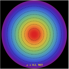
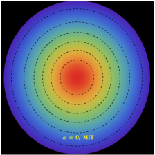
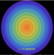
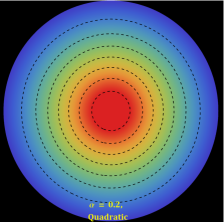
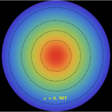
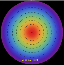
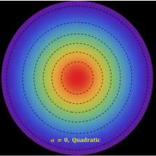
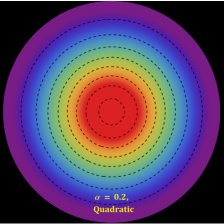
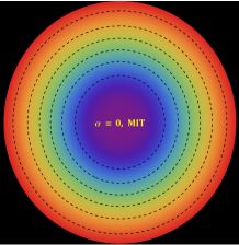
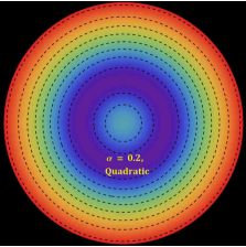
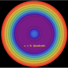
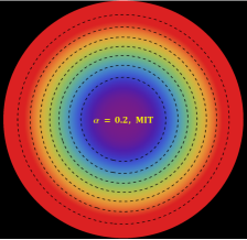
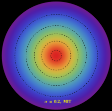
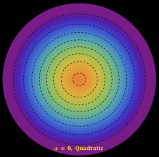
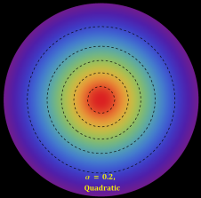
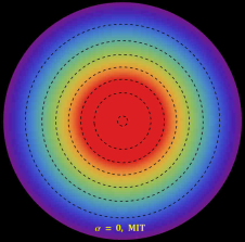
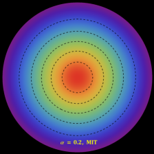
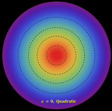
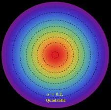
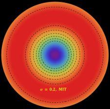
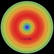
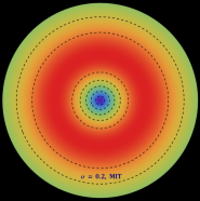
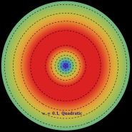
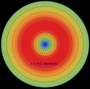
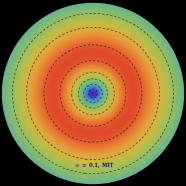
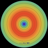
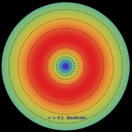
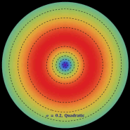
Figure 1: The distribution of energy density [ϵ(r)italic-ϵ𝑟\epsilon(r) in \textkm2]\text{km}^{-2}] versus radial distance r𝑟r from center to boundary of star for MIT Bag model by taking a=0𝑎0a=0 and g=60MeV/fm3subscript𝑔60𝑀𝑒𝑉𝑓superscript𝑚3\mathcal{B}_{g}=60\,MeV/fm^{3} (first two panels) and quadratic model by taking a=5\textkm2𝑎5\text𝑘superscript𝑚2a=5\,\text{km}^{2} and g=60MeV/fm3subscript𝑔60𝑀𝑒𝑉𝑓superscript𝑚3\mathcal{B}_{g}=60\,MeV/fm^{3} [1MeV/fm3=1.3234×106\textkm21𝑀𝑒𝑉𝑓superscript𝑚31.3234superscript106\text𝑘superscript𝑚21\,MeV/fm^{3}=1.3234\times 10^{-6}~{}\text{km}^{-2}] (right two panels) with two different values of α𝛼\alpha for solution 3.1 (ρ=θ00)\rho=\theta^{0}_{0})). We have chosen the following fixed values of constants L=0.0011/\textkm2𝐿0.0011\text𝑘superscript𝑚2L=0.0011/\text{km}^{2}, N=0.00787/\textkm2𝑁0.00787\text𝑘superscript𝑚2N=0.00787/\text{km}^{2}, radius R=12.5\textkm𝑅12.5\text𝑘𝑚R=12.5\,\text{km}, β1=1.1subscript𝛽11.1\beta_{1}=1.1, and β2=1046/\textkm2subscript𝛽2superscript1046\text𝑘superscript𝑚2\beta_{2}=10^{-46}/\text{km}^{2} to plot these curves. The color bar shows the amount of energy density [ϵ(r)italic-ϵ𝑟\epsilon(r) in \textkm2]\text{km}^{-2}] for r=0𝑟0r=0 to r=12.5\textkm𝑟12.5\text𝑘𝑚r=12.5~{}\text{km}.
Refer to caption
Refer to caption
Refer to caption
Refer to caption
Refer to caption
Refer to caption
Refer to caption
Refer to caption
Figure 2: The distribution of radial pressure [Pr(r)subscript𝑃𝑟𝑟P_{r}(r) in \textkm2]\text{km}^{-2}] versus radial distance r𝑟r from center to boundary of star for MIT Bag model by taking a=0𝑎0a=0 and g=60MeV/fm3subscript𝑔60𝑀𝑒𝑉𝑓superscript𝑚3\mathcal{B}_{g}=60\,MeV/fm^{3} (first two panels) and quadratic model by taking a=5\textkm2𝑎5\text𝑘superscript𝑚2a=5\,\text{km}^{2} and g=60MeV/fm3subscript𝑔60𝑀𝑒𝑉𝑓superscript𝑚3\mathcal{B}_{g}=60\,MeV/fm^{3} (right two panels) with two different values of α𝛼\alpha for solution 3.1 (ρ=θ00)\rho=\theta^{0}_{0})). The same values of constants are employed here as used in Fig.3. The color bar shows the amount of radial pressure [Pr(r)subscript𝑃𝑟𝑟P_{r}(r) in \textkm2]\text{km}^{-2}] for r=0𝑟0r=0 to r=12.5\textkm𝑟12.5\text𝑘𝑚r=12.5~{}\text{km}.
Refer to caption
Refer to caption
Refer to caption
Refer to caption
Refer to caption
Refer to caption
Refer to caption
Refer to caption
Figure 3: The distribution of anisotropy [Δ(r)Δ𝑟\Delta(r) in \textkm2]\text{km}^{-2}] versus radial distance r𝑟r from center to boundary of star for MIT Bag model by taking a=0𝑎0a=0 and g=60MeV/fm3subscript𝑔60𝑀𝑒𝑉𝑓superscript𝑚3\mathcal{B}_{g}=60\,MeV/fm^{3} (first two panels) and quadratic model by taking a=5\textkm2𝑎5\text𝑘superscript𝑚2a=5\,\text{km}^{2} and g=60MeV/fm3subscript𝑔60𝑀𝑒𝑉𝑓superscript𝑚3\mathcal{B}_{g}=60\,MeV/fm^{3} (right two panels) with two different values of α𝛼\alpha for solution 3.1 (ρ=θ00)\rho=\theta^{0}_{0})). The same values of constants are employed here as used in Fig.3. The color bar shows the amount of anisotropy [Δ(r)Δ𝑟\Delta(r) in \textkm2]\text{km}^{-2}] for r=0𝑟0r=0 to r=12.5\textkm𝑟12.5\text𝑘𝑚r=12.5~{}\text{km}.

5 Physical analysis of completely deformed SS models and astrophysical implications

5.1 Regular behavior of strange star (SS) models

5.1.1 For solution 3.1 (ρ=θ00𝜌subscriptsuperscript𝜃00\rho=\theta^{0}_{0})

We now turn our attention to the physical analysis of the models obtained for the ρ=θ00𝜌subscriptsuperscript𝜃00\rho=\theta^{0}_{0} sector. The energy density is plotted in Fig 1. Keep in mind that for α=0𝛼0\alpha=0 we recover the standard f(𝒬)𝑓𝒬f(\mathcal{Q}) gravity. Starting from the left of Fig. 3. the first and second plots reveal the behavior of the energy density as a function of the radial coordinate for a fluid obeying the MIT bag model EOS. We observe that the energy density is regular at all interior points of the fluid configuration, attaining a maximum at the center. It is clear that contributions from the decoupling constant, α𝛼\alpha leads to higher core densities in the linear regime as compared to the standard f(𝒬)𝑓𝒬f(\mathcal{Q}) gravity models. The third and fourth panels reveal the trend in the energy density for a fluid obeying a quadratic EOS. We note that for the quadratic EOS, contributions from α𝛼\alpha lead to a significant increase in the energy density, particularly in the central regions of the star. More ever, the closeness of the contours reveals that these higher densities lead to more compact configurations. If we compare the linear EOS to the quadratic EOS for nonzero decoupling constant, we observe that stars with quadratic EOS have higher core densities and are more compact than their linear EOS counterparts. Panels one and three reveal that in the absence of the decoupling constant (α=0)𝛼0(\alpha=0), the energy density in the linear regime dominates its quadratic counterpart. The linear model predicts high core densities but as one moves to the surface layers of the star, the densities are of similar magnitude. A comparison of panels 2 and 4 (MIT versus quadratic EOS for nonvanishing decoupling parameter) reveals the density for the quadratic model is higher than the linear model at each interior point of the bounded configuration.

We now consider the trends in the behaviour of the radial pressure (plotted in Fig. 3) throughout the interior of the compact object for the ρ=θ00𝜌subscriptsuperscript𝜃00\rho=\theta^{0}_{0} sector. A comparison of panels one and three show that the pressure in the quadratic models dominate over the linear models when the decoupling parameter vanishes. This increased pressure in the quadratic models leads to greater stability against the inwardly driven gravitational force, with this effect being enhanced in the central regions of the star. The surface pressure in the quadratic models dominates their linear counterparts thus leading to stable surface layers. It is clear from the second and fourth panels that the pressure is enhanced in the presence of the decoupling parameter. In addition, the radial pressure in the quadratic models dominates their linear counterparts at each interior point from the center through to the stellar surface with the highest pressures achieved in models with quadratic EOS and nonzero α𝛼\alpha.

Before we embark on a discussion of the trends in anisotropy in our models, we highlight some work which motivates the inclusion of pressure anisotropy in stellar configurations. In our models the radial and transverse stresses at each interior point of the compact object are unequal. Obviously, equality of the transverse component of pressure does ensure the spherical symmetry of the model (Dev & Gleiser, 2002). However, there are various reasons for consideration of the origin of anisotropy inside the compact stars (Ruderman, 1972; Sawyer, 1972; Jones, 1975; Sokolov, 1980; Kippenhahn & Weigert, 1990; Weber, 1999; Liebling & Palenzuela, 2012) and review work on the local anisotropy by Herrera & Santos (1997) may be informative in this regard. Very recently, Hererra (2020) has investigated the conditions for the (in)stability of the isotropic pressure condition in collapsing spherically symmetric, dissipative fluid distributions. Herrera demonstrated that an initially isotropic configuration upon leaving hydrostatic equilibrium evolves into an anisotropic regime.

The anisotropy parameter is displayed in Fig. 3. We observe that the anisotropy changes sign within the compact object. We recall that a positive anisotropy factor signifies a repulsive anisotropic force which is directed outwards (Hansraj et al., 2022). This helps stabilise the stellar configuration against gravity. In Fig. 3, the extreme left panel shows that the anisotropy parameter is minimum at the centre of the fluid and is negative up to a finite radius, r0subscript𝑟0r_{0}. This negative anisotropic factor is accompanied by an inwardly driven force which sums with the gravitational force, leading to an unstable interior. As one moves beyond r=r0𝑟subscript𝑟0r=r_{0}, the anisotropy factor becomes positive. The repulsive force associated with Δ>0Δ0\Delta>0 stabilises the surface layers of the star. In direct comparison, panel 3 reveals a peculiar behaviour of the anisotropy factor. It starts off negative in the central regions and remains negative up to a large radius, r1subscript𝑟1r_{1} where r1>r0subscript𝑟1subscript𝑟0r_{1}>r_{0}. It appears that the quadratic EOS model is more unstable than its linear counterpart in the central regions of the compact object. As one moves further out, the anisotropy becomes positive. The first and third panels indicate that the quadratic EOS model has a narrower band of stable surface layers as compared to the linear EOS model. Its quadratic counterpart with a vanishing decoupling parameter (third panel) shows a marked difference between the two models. In the quadratic model, we see an interesting variation in the anisotropy parameter, i.e., starting from the centre of the star, the anisotropy is negative for some central region, 0<r<r00𝑟subscript𝑟00<r<r_{0} then becomes more negative as one moves outwards towards the boundary. The anisotropy remains negative for r0<r<r1subscript𝑟0𝑟subscript𝑟1r_{0}<r<r_{1} where r1>r0subscript𝑟1subscript𝑟0r_{1}>r_{0}. Beyond r1subscript𝑟1r_{1}, the anisotropy becomes positive, rendering the surface layers stable due to the repulsive anisotropic force. The change in sign of ΔΔ\Delta within the quadratic EOS model can be attributed to phase transitions in different regions within the stellar fluid. In the second and fourth panels, we observe the effect of a nonvanishing decoupling constant in both the linear and quadratic EOS models, respectively. In the second panel, we observe that Δ<0Δ0\Delta<0 from the centre to some finite radius. Thereafter, ΔΔ\Delta remains positive up to the boundary of the star. The fourth panel shows that anisotropy is negative within the central regions of the configuration. The anisotropy factor starts off with a finite negative value from r=0𝑟0r=0 up to some radius r=r0𝑟subscript𝑟0r=r_{0}. Thereafter ΔΔ\Delta becomes more negative as one move outwards. After some radius, r1subscript𝑟1r_{1} the anisotropy factor changes sign and becomes positive. A comparison of the second and fourth panels clearly shows that the surface layers of the linear model are more stable than their quadratic counterpart. It is interesting to observe the behavior of the anisotropy in the quadratic models, particularly the change of sign of ΔΔ\Delta in different regions within the stellar fluid. The change in the nature of the anisotropic force (from attraction to repulsion) leads to an unstable core but stable surface layers. This interesting behavior in anisotropy was also observed (Maurya et al., 2023). In this work, they modeled compact objects in f(𝒬)𝑓𝒬f(\mathcal{Q}) gravity in which the stellar fluid obeyed the MIT bag model EOS.
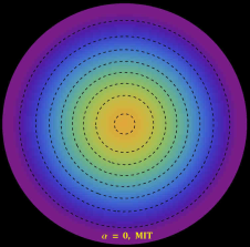
Refer to caption
Refer to caption
Refer to caption
Refer to caption
Refer to caption
Refer to caption
Refer to caption
Refer to caption
Figure 4: The distribution of energy density [ϵ(r)italic-ϵ𝑟\epsilon(r) in \textkm2]\text{km}^{-2}] versus radial distance r𝑟r from center to boundary of star for MIT Bag model by taking a=0𝑎0a=0 and g=60MeV/fm3subscript𝑔60𝑀𝑒𝑉𝑓superscript𝑚3\mathcal{B}_{g}=60\,MeV/fm^{3} (first two panels) and quadratic model by taking a=2\textkm2𝑎2\text𝑘superscript𝑚2a=2\,\text{km}^{2} and g=60MeV/fm3subscript𝑔60𝑀𝑒𝑉𝑓superscript𝑚3\mathcal{B}_{g}=60\,MeV/fm^{3} (right two panels) with two different values of α𝛼\alpha for solution  3.2(pr=θ11)p_{r}=\theta^{1}_{1})). We have chosen the following fixed values of constants L=0.0011/\textkm2𝐿0.0011\text𝑘superscript𝑚2L=0.0011/\text{km}^{2}, N=0.00787/\textkm2𝑁0.00787\text𝑘superscript𝑚2N=0.00787/\text{km}^{2}, radius R=12.5\textkm𝑅12.5\text𝑘𝑚R=12.5\,\text{km}, β1=1.1subscript𝛽11.1\beta_{1}=1.1, and β2=1046/\textkm2subscript𝛽2superscript1046\text𝑘superscript𝑚2\beta_{2}=10^{-46}/\text{km}^{2} to plot these curves. The color bar shows the amount of energy density [ϵ(r)italic-ϵ𝑟\epsilon(r) in \textkm2]\text{km}^{-2}] for r=0𝑟0r=0 to r=12.5\textkm𝑟12.5\text𝑘𝑚r=12.5~{}\text{km}.
Refer to caption
Refer to caption
Refer to caption
Refer to caption
Refer to caption
Refer to caption
Refer to caption
Refer to caption
Figure 5: The distribution of radial pressure [Pr(r)subscript𝑃𝑟𝑟P_{r}(r) in \textkm2]\text{km}^{-2}] versus radial distance r𝑟r from center to boundary of star for MIT Bag model by taking a=0𝑎0a=0 and g=60MeV/fm3subscript𝑔60𝑀𝑒𝑉𝑓superscript𝑚3\mathcal{B}_{g}=60\,MeV/fm^{3} (first two panels) and quadratic model by taking a=2\textkm2𝑎2\text𝑘superscript𝑚2a=2\,\text{km}^{2} and g=60MeV/fm3subscript𝑔60𝑀𝑒𝑉𝑓superscript𝑚3\mathcal{B}_{g}=60\,MeV/fm^{3} (right two panels) with two different values of α𝛼\alpha for solution 3.2 (pr=θ11)p_{r}=\theta^{1}_{1})). The same values of constants are employed here as used in Fig.6. The color bar shows the amount of radial pressure [Pr(r)subscript𝑃𝑟𝑟P_{r}(r) in \textkm2]\text{km}^{-2}] for r=0𝑟0r=0 to r=12.5\textkm𝑟12.5\text𝑘𝑚r=12.5~{}\text{km}.
Refer to caption
Refer to caption
Refer to caption
Refer to caption
Refer to caption
Refer to caption
Refer to caption
Refer to caption
Figure 6: The distribution of anisotropy [Δ(r)Δ𝑟\Delta(r) in \textkm2]\text{km}^{-2}] versus radial distance r𝑟r from center to boundary of star for MIT Bag model by taking a=0𝑎0a=0 and g=60MeV/fm3subscript𝑔60𝑀𝑒𝑉𝑓superscript𝑚3\mathcal{B}_{g}=60\,MeV/fm^{3} (first two panels) and quadratic model by taking a=2\textkm2𝑎2\text𝑘superscript𝑚2a=2\,\text{km}^{2} and g=60MeV/fm3subscript𝑔60𝑀𝑒𝑉𝑓superscript𝑚3\mathcal{B}_{g}=60\,MeV/fm^{3} (right two panels) with two different values of α𝛼\alpha for solution 3.2 (pr=θ11)p_{r}=\theta^{1}_{1})). The same values of constants are employed here as used in Fig.6. The color bar shows the amount of anisotropy [Δ(r)Δ𝑟\Delta(r) in \textkm2]\text{km}^{-2}] for r=0𝑟0r=0 to r=12.5\textkm𝑟12.5\text𝑘𝑚r=12.5~{}\text{km}.

5.1.2 For solution 3.2 (pr=θ11subscript𝑝𝑟subscriptsuperscript𝜃11p_{r}=\theta^{1}_{1})

In this subsection, we move our attention to the physical analysis of the models discovered for the solution pr=θ11subscript𝑝𝑟subscriptsuperscript𝜃11p_{r}=\theta^{1}_{1}. Figure 6 exhibits the energy density plot. As usual α=0𝛼0\alpha=0 leads to the standard f(𝒬)𝑓𝒬f(\mathcal{Q}) gravity. Initially, let us look at the left two panels of Fig. 6, the first and second plots show the behavior of the energy density against the radial coordinate r𝑟r for a fluid distribution following the MIT bag model EOS. It is evident that the energy density obtained here is regular at all internal points of the stellar structure and attaining a maximum at the core of the object. From the first and second panels, it is clear that the contribution of the decoupling constant (α𝛼\alpha) allows a higher core densities in the MIT bag model EOS as compared to the pure f(𝒬)𝑓𝒬f(\mathcal{Q}) gravity stellar models. Furthermore, the third and fourth panels indicate the trend in the energy density for the fluid distribution in the quadratic EOS. We notice that the contributions from α𝛼\alpha in the context of quadratic EOS gives to a substantial growth in the energy density, particularly in the central regions of the star which lead to more compact configurations. On the other hand, we also detect that stars obeying quadratic EOS have higher central densities and are more compact than their linear EOS counterparts as happened in the first solution.
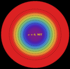
Now we move to the Fig. 6 to check the behavior of the radial pressure within the stellar object for the pr=θ11subscript𝑝𝑟subscriptsuperscript𝜃11p_{r}=\theta^{1}_{1} sector. On comparing of the panels to the first and third in absence of the gravitational decoupling, we observe that the radial pressure of models under the quadratic EOS dominates over models in a linear regime. Furthermore, this increment in the pressure for quadratic models leads to greater stability in the central regions of the star against the inwardly directed gravitational force. From the second and fourth panels, it is clear that the pressure decreases in the presence of the gravitational decoupling parameter. Apart from this, the radial pressure of the model in the context of quadratic EOS dominates their linear counterparts everywhere inside the star from the center to the surface as well as the highest pressure is achieved in models obeying quadratic EOS under vanishing α𝛼\alpha.

A scrutiny of Fig. 6 reveals that the anisotropy is regular at all interior points of each of the models displayed in the four panels. In addition, the anisotropy is positive and increases from the center of the star toward the boundary. This is in direct contrast to our models ρ=θ00𝜌subscriptsuperscript𝜃00\rho=\theta^{0}_{0} sector. A comparison of panels 1 and 3, shows the trend in anisotropy in the absence of the decoupling constant for the linear and quadratic EOS respectively. The central anisotropy is lower in the linear model compared to its quadratic counterpart. As one approaches the surface layers, we observe that anisotropy increases, with the increase more significant over a larger portion of the surface layers in the linear model. Since Δ>0Δ0\Delta>0, the repulsive anisotropic renders the surface layers more stable than the central core regions. Comparatively, the relative magnitudes of the anisotropy show that the linear model is more stable than the quadratic model for the vanishing decoupling parameter. We now turn our attention to the second and third panels of Fig. 6. In these models, the anisotropy increases from the center of the configuration toward the boundary. The increase in ΔΔ\Delta is more profound at each interior point in the linear model. This indicates that the contribution from the repulsive nature of the anisotropic force renders the linear model more stable. A peculiar observation in the behavior of the anisotropy is observed in the linear model. While the contributions from anisotropy increase steadily from the center, r0subscript𝑟0r_{0} to some finite radius r1subscript𝑟1r_{1}, we observe a decrease in ΔΔ\Delta for r1<rbsubscript𝑟1𝑟𝑏r_{1}<r\leq b. This trend is not observed in the quadratic model. If we now compare panels 1 and 2, ie., the linear models for α=0𝛼0\alpha=0 and nonvanishingα𝛼\alpha, respectively, we observe that the decoupling parameter stabilizes the central region by enhancing the anisotropy. A comparison of panels 3 and 4 clearly shows the effect of the decoupling parameter on ΔΔ\Delta in the quadratic models. We note that the contributions from α𝛼\alpha lead to enhanced anisotropy throughout the stellar configuration thus leading to greater stability of concentric matter shells centered about the origin. .

Refer to caption
Refer to caption
Figure 7: The above MR𝑀𝑅M-R curves are plotted for describing the upper limit of mass-radius relationship in a purely MIT bag model (a=0𝑎0a=0) for different b𝑏b with fixed a=0,α=0.3\textkm2formulae-sequence𝑎0𝛼0.3\text𝑘superscript𝑚2a=0,~{}\alpha=0.3\,\text{km}^{2} and g=60MeV/fm3subscript𝑔60𝑀𝑒𝑉𝑓superscript𝑚3\mathcal{B}_{g}=60\,MeV/fm^{3} for solution 3.1 (θ00=ρsubscriptsuperscript𝜃00𝜌\theta^{0}_{0}=\rho) - (left panel) and with fixed a=0,α=0.2\textkm2formulae-sequence𝑎0𝛼0.2\text𝑘superscript𝑚2a=0,~{}\alpha=0.2\,\text{km}^{2} and g=60MeV/fm3subscript𝑔60𝑀𝑒𝑉𝑓superscript𝑚3\mathcal{B}_{g}=60\,MeV/fm^{3} solution 3.2 (θ11=prsubscriptsuperscript𝜃11subscript𝑝𝑟\theta^{1}_{1}=p_{r})   (right panel), respectively.
Refer to caption
Refer to caption
Figure 8: The above MR𝑀𝑅M-R curves are plotted for describing the upper limit of mass-radius relationship in MIT-Model for different α𝛼\alpha with fixed a=0,b=1/3formulae-sequence𝑎0𝑏13a=0,~{}b=1/3 and g=60MeV/fm3subscript𝑔60𝑀𝑒𝑉𝑓superscript𝑚3\mathcal{B}_{g}=60\,MeV/fm^{3} for solution 3.1 in (θ00=ρsubscriptsuperscript𝜃00𝜌\theta^{0}_{0}=\rho) - (left panel) and solution 3.2 in (θ11=prsubscriptsuperscript𝜃11subscript𝑝𝑟\theta^{1}_{1}=p_{r})   (right panel), respectively.
Refer to caption
Refer to caption
Figure 9: The above MR𝑀𝑅M-R curves are plotted for describing the upper limit of mass-radius relationship in Quadratic+MIT bag model for different a𝑎a with fixed α=0.3\textkm2𝛼0.3\text𝑘superscript𝑚2\alpha=0.3\,\text{km}^{2}, b=1/3𝑏13b=1/3 and g=60MeV/fm3subscript𝑔60𝑀𝑒𝑉𝑓superscript𝑚3\mathcal{B}_{g}=60\,MeV/fm^{3} for solution 3.1 (θ00=ρsubscriptsuperscript𝜃00𝜌\theta^{0}_{0}=\rho) - (left panel) and α=0.2\textkm2𝛼0.2\text𝑘superscript𝑚2\alpha=0.2\,\text{km}^{2}, b=1/3𝑏13b=1/3 and g=60MeV/fm3subscript𝑔60𝑀𝑒𝑉𝑓superscript𝑚3\mathcal{B}_{g}=60\,MeV/fm^{3} solution 3.2 (θ11=prsubscriptsuperscript𝜃11subscript𝑝𝑟\theta^{1}_{1}=p_{r}) - (right panel), respectively.
Refer to caption
Refer to caption
Figure 10: The above MR𝑀𝑅M-R curve is plotted for describing the upper limit of mass-radius relationship in quadratic+MIT bag model for different b𝑏b with fixed α=0.2\textkm2𝛼0.2\text𝑘superscript𝑚2\alpha=0.2\,\text{km}^{2}, a=2\textkm2𝑎2\text𝑘superscript𝑚2a=2\,\text{km}^{2} and g=60MeV/fm3subscript𝑔60𝑀𝑒𝑉𝑓superscript𝑚3\mathcal{B}_{g}=60\,MeV/fm^{3} (left panel) while the right panel shows a quadratic+MIT bag model for different α𝛼\alpha with fixed a=2\textkm2𝑎2\text𝑘superscript𝑚2a=2\,\text{km}^{2}, b=1/3𝑏13b=1/3 and g=60MeV/fm3subscript𝑔60𝑀𝑒𝑉𝑓superscript𝑚3\mathcal{B}_{g}=60\,MeV/fm^{3} for the solution 3.2 (θ11=prsubscriptsuperscript𝜃11subscript𝑝𝑟\theta^{1}_{1}=p_{r}).

5.2 Constraining upper limit of maximum mass for SS via M-R diagrams

In this section we investigate the effect of the decoupling parameter (α𝛼\alpha), bag constant (gsubscript𝑔\mathcal{B}_{g}) and EOS parameters on the mass-radius relations of various compact objects and compare our theoretical values to observational constraints. Based on the EOS

prsubscript𝑝𝑟\displaystyle p_{r} =\displaystyle= aρ1+1/n+bρ+c,𝑎superscript𝜌11𝑛𝑏𝜌𝑐\displaystyle a\,\rho^{1+1/n}+b\rho+c, (95)

we classify the stellar fluid as

  • (1)

    a0,b0formulae-sequence𝑎0𝑏0absenta\neq 0,b\neq 0\rightarrow quadratic EOS

  • (2)

    a0,b=0formulae-sequence𝑎0𝑏0absenta\neq 0,b=0\rightarrow pure quadratic EOS

  • (3)

    a=0,b0formulae-sequence𝑎0𝑏0absenta=0,b\neq 0\rightarrow linear EOS (MIT bag model)

5.2.1 Linear EOS with constancy in bag constant, fixed decoupling parameter and varying EOS parameter

We have up to this point tested the physical viability of our solutions in describing self-gravitating stellar objects. We have shown, through tests based on regularity, causality, and stability that these solutions describe physically realizable stellar configurations. In this section, we constrain the free parameters in our solutions by using observational data of compact stars LMC X-4, Cen X-3, PSR J1614-2230, PSR J0740+6620, and the supposedly secondary component of GW190814. The robustness of our solutions allows us to predict the observed mass-radius relations of these stars. Starting off with solution A emanating from the ρ=θ00𝜌subscriptsuperscript𝜃00\rho=\theta^{0}_{0} sector, we refer to Table 3 and Fig. 7 (left panel). Here we focus on the MIT-bag models where we have fixed the Bag constant and decoupling parameter while varying the linear EOS parameter, b𝑏b. At the outset we must point out that a fixed linear EOS parameter b𝑏b, leads to the prediction of a category of stars with similar trends in mass and radii and not individual stars. From Table 3, we observe that for small values of b𝑏b, i.e., linear contributions from the energy density, do account for low-mass stars such as LMC X-4 and Cen X-3. Our model shows that by fixing the parameter b𝑏b, we can obtain masses of stars beyond 2 Msubscript𝑀direct-productM_{\odot} . For example, for b=0.38𝑏0.38b=0.38, our model predicts the existence of a class of stars befitting of the secondary component of the GW190814 event with a mass range of 2.5-2.67 Msubscript𝑀direct-productM_{\odot} and a radius of 15.74+0.400.21superscriptsubscriptabsent0.210.40{}_{-0.21}^{+0.40}. On the right panel, we see the trend in the M-R curves for the pr=θ11subscript𝑝𝑟subscriptsuperscript𝜃11p_{r}=\theta^{1}_{1} sector in the linear regime. A similar trend in the increase in the linear EOS parameter on the radii of compact stars is observed in this case. However, there is one notable difference, while the predicted radii increase as b𝑏b increases, the pr=θ11subscript𝑝𝑟subscriptsuperscript𝜃11p_{r}=\theta^{1}_{1} sector predicts smaller radii, i.e., more compact stellar models. For example, in the case of the GW190814 event, the secondary component has a radius of 14.02+0.090.08superscriptsubscriptabsent0.080.09{}_{-0.08}^{+0.09} km for the upper value of b𝑏b, which is 10%percent1010\% less than its ρ=θ00𝜌subscriptsuperscript𝜃00\rho=\theta^{0}_{0} counterpart.

5.2.2 Linear EOS with constancy in bag constant, fixed EOS parameter and varying decoupling constant

We now look at Table 3 in conjunction with Figure 8 in which we have fixed the bag constant and the EOS parameter, b𝑏b while varying α𝛼\alpha. From Table 3 and the left panel of Fig. 8, we observe that an increase in the decoupling parameter results in a decrease in radii leading to more compact configurations. A similar trend is observed in the pr=θ11subscript𝑝𝑟subscriptsuperscript𝜃11p_{r}=\theta^{1}_{1} sector. We also observe that for the chosen values of the bag constant and EOS parameter, our solutions are able to predict a wider range of radii for all compact objects under investigation. A comparison of the left and right panels reveal that the allowable radii for the compact objects under investigation is more tightly bounded for the ρ=θ00𝜌subscriptsuperscript𝜃00\rho=\theta^{0}_{0} sector. The left panel shows that low mass stars such as LMC X-4 (1.29 ±plus-or-minus\pm 0.05 Msubscript𝑀direct-productM_{\odot}) and Cen X-3 (1.49 ±plus-or-minus\pm 0.08 Msubscript𝑀direct-productM_{\odot}) exist for radii greater 10 km. For the pr=θ11subscript𝑝𝑟subscriptsuperscript𝜃11p_{r}=\theta^{1}_{1}, there is wider range of radii for low mass stars closer to 9 km. More noticeably is the prediction of the existence of higher-mass compact objects beyond 2 Msubscript𝑀direct-productM_{\odot}. For small α𝛼\alpha, there exist stars with masses closer to 3 Msubscript𝑀direct-productM_{\odot}. For the vanishing of the decoupling parameter (α=0𝛼0\alpha=0), stellar masses exceed 3 Msubscript𝑀direct-productM_{\odot}. For the right panel, we note that the maximum mass is in the order of 3.5 Msubscript𝑀direct-productM_{\odot}. In a study of Burgio et al. (Burgio et al., 2018), they questioned the existence of compact stars with small radii giving rise to the GW170817/AT2017gfo𝐺𝑊170817𝐴𝑇2017𝑔𝑓𝑜GW170817/AT2017gfo signals. In one of their proposals, the so-called ‘twin-star’ scenario they concluded that the merger involved the coalescence of a hadronic star and a quark matter star with radii in the range 10.7\textkm<R1.5<12\textkm10.7\text𝑘𝑚subscript𝑅1.512\text𝑘𝑚10.7\text{km}<R_{1.5}<12\text{km} with R1.5subscript𝑅1.5R_{1.5} (14.2815.4114.2815.4114.28-15.41 km for θ00=ρsubscriptsuperscript𝜃00𝜌\theta^{0}_{0}=\rho and 9.7014.189.7014.189.70-14.18 km for θ11=prsubscriptsuperscript𝜃11subscript𝑝𝑟\theta^{1}_{1}=p_{r}) being the radius of a 1.5 Msubscript𝑀direct-productM_{\odot} compact star. Figure 8 accounts for the existence of a myriad of observed compact objects including those falling into the ‘twin star’ category scenario with the latter being more suitable for pr=θ11subscript𝑝𝑟subscriptsuperscript𝜃11p_{r}=\theta^{1}_{1} sector.

5.2.3 Quadratic EOS with fixed bag constant, fixed decoupling constant with varying quadratic EOS parameter

Here we focus on Table 3. and Figure 9. It is clear in this scenario, both of our solutions do not predict very well the existence of compact objects beyond 2 Msubscript𝑀direct-productM_{\odot}. Even in the case of PSR J1614-2230 with a mass of 1.97±plus-or-minus\pm0.04 Msubscript𝑀direct-productM_{\odot}, which is less than the 2.0 Msubscript𝑀direct-productM_{\odot}, fails to exist. The lower mass stars have larger radii, thus indicating that these candidates have low densities compared to their linear EOS counterparts as displayed in Figure 8. In a study by (Astashenok et al., 2020), they showed that the observations of GW190814 can be accounted for within the framework of f(R)𝑓𝑅f(R) gravity and the inclusion of rotation. They utilized three frameworks, i.e., classical GR, f(R)𝑓𝑅f(R) gravity with f(R)=R+αR2𝑓𝑅𝑅𝛼superscript𝑅2f(R)=R+\alpha R^{2}, where α𝛼\alpha is quadratic curvature correction and finally f(R)=R1+ϵ𝑓𝑅superscript𝑅1italic-ϵf(R)=R^{1+\epsilon} where ϵitalic-ϵ\epsilon is a measure of a small deviation from GR. Utilizing different EOS’s, they showed that in the absence of rotation, the models of compact objects for both GR and f(R)𝑓𝑅f(R) gravity with varying α𝛼\alpha lead to masses less than 2.5 Msubscript𝑀direct-productM_{\odot} and radii between 10 and 14 km. With the inclusion of rotation, the f(R)𝑓𝑅f(R) models can easily account for masses greater than 2.5 Msubscript𝑀direct-productM_{\odot} this accounting for the observed mass of the secondary component of GW190814. For observed rotational frequencies of neutron stars, f(R)𝑓𝑅f(R) gravity predicts the existence of a 2.0 Msubscript𝑀direct-productM_{\odot} compact object. In the case of f(R)=R1+ϵ𝑓𝑅superscript𝑅1italic-ϵf(R)=R^{1+\epsilon} framework, they obtained masses in the range of 2.5- 2.67 Msubscript𝑀direct-productM_{\odot} for ϵitalic-ϵ\epsilon in the range 0.005 and 0.008. Interestingly, the radii of these compact objects in f(R)𝑓𝑅f(R) gravity with rotation can vary between 12 to 18 km. We have also obtained models of compact objects with large radii in this category of stars.

5.2.4 Quadratic EOS with fixed bag constant, fixed quadratic EOS parameter with constant versus varying decoupling constant for mimicking of radial pressure, pr=θ11subscript𝑝𝑟subscriptsuperscript𝜃11p_{r}=\theta^{1}_{1}

In this subsection, we pay particular attention to the M-R curves arising in the composite linear-quadratic EOS and the effect of the decoupling constant. Table 4. shows that these models predict the existence of low-mass stars with an increase in the decoupling constant leading to higher-mass stars with larger radii very similar to the trends obtained by (Astashenok et al., 2021) in describing rotating neutron stars in f(R)=R+αR2𝑓𝑅𝑅𝛼superscript𝑅2f(R)=R+\alpha R^{2} gravity. It is clear from Table 4 and Figure 10 that the mixed EOS model fails to predict masses which can account for the LIGO observation of approximately 2.6 Msubscript𝑀direct-productM_{\odot} of the secondary component of the binary coalescence GW190814. It appears that when the linear and quadratic EOS parameters are switched on simultaneously, the decoupling constant quenches any increase in the mass of the compact object. While these models fail to predict masses above 2.6 Msubscript𝑀direct-productM_{\odot}, the quadratic EOS predicts the existence of well-known pulsars and neutron stars to a very good approximation.

In comparing the models derived from the ρ=θ00𝜌subscriptsuperscript𝜃00\rho=\theta^{0}_{0} and pr=θ11subscript𝑝𝑟subscriptsuperscript𝜃11p_{r}=\theta^{1}_{1} sectors we compared and contrasted their predicting powers when it comes to low mass stars as well as extreme masses bordering on the mass of the lightest black hole. We have shown that the predicted stellar masses are sensitive to the decoupling constant, α𝛼\alpha, the linear EOS parameter, b𝑏b, the quadratic EOS parameter, a𝑎a, and the bag constant. By varying these constants in particular sets, our models describe a family of compact objects with varying EOS’s ranging from the simplest linear EOS (MIT bag model), through to the pure quadratic EOS and the more complex quadratic EOS. The tabulated data and plots reveal that the quadratic EOS accounts for a wide spectrum of observed compact objects in the low-mass limit and stars which qualify as the secondary component of the GW190814 event.

Table 1: The predicted radii of compact stars LMC X-4, Cen X-3, PSR J1614-2230, PSR J0740+6620, and GW190814 for MIT-bag model (see Fig.7).
Objects MM𝑀subscript𝑀direct-product\frac{M}{M_{\odot}} Predicted R𝑅R km Predicted R𝑅R km
For solution ρ=θ00𝜌subscriptsuperscript𝜃00\rho=\theta^{0}_{0} For solution pr=θ11subscript𝑝𝑟subscriptsuperscript𝜃11p_{r}=\theta^{1}_{1}
b=0.18𝑏0.18b=0.18 b=0.23𝑏0.23b=0.23 b=0.28𝑏0.28b=0.28 b=0.33𝑏0.33b=0.33 b=0.38𝑏0.38b=0.38 b=0.13𝑏0.13b=0.13 b=0.18𝑏0.18b=0.18 b=0.23𝑏0.23b=0.23 b=0.28𝑏0.28b=0.28 b=0.33𝑏0.33b=0.33
LMC X-4 (Rawls et al., 2011) 1.29 ±plus-or-minus\pm 0.05 9.390.48+0.24superscriptsubscript9.390.480.249.39_{-0.48}^{+0.24} 11.650.01+0.02superscriptsubscript11.650.010.0211.65_{-0.01}^{+0.02} 13.010.08+0.06superscriptsubscript13.010.080.0613.01_{-0.08}^{+0.06} 14.050.1+0.1superscriptsubscript14.050.10.114.05_{-0.1}^{+0.1} 14.940.10+0.12superscriptsubscript14.940.100.1214.94_{-0.10}^{+0.12} 8.230.04+0.06superscriptsubscript8.230.040.068.23_{-0.04}^{+0.06} 9.450.11+0.05superscriptsubscript9.450.110.059.45_{-0.11}^{+0.05} 10.320.09+0.11superscriptsubscript10.320.090.1110.32_{-0.09}^{+0.11} 11.050.11+0.10superscriptsubscript11.050.110.1011.05_{-0.11}^{+0.10} 11.670.13+0.13superscriptsubscript11.670.130.1311.67_{-0.13}^{+0.13}
Cen X-3 (Rawls et al., 2011) 1.49±plus-or-minus\pm0.08 - 11.630.06+0.13superscriptsubscript11.630.060.1311.63_{-0.06}^{+0.13} 13.25+0.050.08superscriptsubscriptabsent0.080.05{}_{-0.08}^{+0.05} 14.44+0.120.14superscriptsubscriptabsent0.140.12{}_{-0.14}^{+0.12} 15.43+0.140.16superscriptsubscriptabsent0.160.14{}_{-0.16}^{+0.14} 8.45+0.020.08superscriptsubscriptabsent0.080.02{}_{-0.08}^{+0.02} 9.790.06+0.09superscriptsubscript9.790.060.099.79_{-0.06}^{+0.09} 10.72+0.130.14superscriptsubscriptabsent0.140.13{}_{-0.14}^{+0.13} 11.55+0.160.19superscriptsubscriptabsent0.190.16{}_{-0.19}^{+0.16} 12.210.18+0.18superscriptsubscript12.210.180.1812.21_{-0.18}^{+0.18}
PSR J1614-2230 (Demorest et al., 2010) 1.97±plus-or-minus\pm0.04 - - 12.89+0.170.11superscriptsubscriptabsent0.110.17{}_{-0.11}^{+0.17} 14.81+0.010.01superscriptsubscriptabsent0.010.01{}_{-0.01}^{+0.01} 16.11+0.010.02superscriptsubscriptabsent0.020.01{}_{-0.02}^{+0.01} - 10.210.01+0.02superscriptsubscript10.210.010.0210.21_{-0.01}^{+0.02} 11.44+0.050.05superscriptsubscriptabsent0.050.05{}_{-0.05}^{+0.05} 12.39+0.070.04superscriptsubscriptabsent0.040.07{}_{-0.04}^{+0.07} 13.210.06+0.05superscriptsubscript13.210.060.0513.21_{-0.06}^{+0.05}
PSR J0740+6620 (Cromartie et al., 2019) 2.140.17+0.2subscriptsuperscript2.140.20.172.14^{+0.2}_{-0.17} - - - 14.68+0.130.57superscriptsubscriptabsent0.570.13{}_{-0.57}^{+0.13} 16.18+0.020.10superscriptsubscriptabsent0.100.02{}_{-0.10}^{+0.02} - 10.19+0.010.53superscriptsubscriptabsent0.530.01{}_{-0.53}^{+0.01} 11.63+0.080.21superscriptsubscriptabsent0.210.08{}_{-0.21}^{+0.08} 12.63+0.200.27superscriptsubscriptabsent0.270.20{}_{-0.27}^{+0.20} 13.470.36+0.27superscriptsubscript13.470.360.2713.47_{-0.36}^{+0.27}
GW190814 (Beniamini & Bonnerot, 2021) 2.5-2.67 - - - - 15.74+0.400.21superscriptsubscriptabsent0.210.40{}_{-0.21}^{+0.40} - - 11.64+0.130.07superscriptsubscriptabsent0.070.13{}_{-0.07}^{+0.13} 13.03+0.020.06superscriptsubscriptabsent0.060.02{}_{-0.06}^{+0.02} 14.02+0.090.08superscriptsubscriptabsent0.080.09{}_{-0.08}^{+0.09}
Table 2: The predicted radii of compact stars LMC X-4, Cen X-3, PSR J1614-2230, PSR J0740+6620, and GW190814 for MIT-bag model (see Fig.8).
Objects MM𝑀subscript𝑀direct-product\frac{M}{M_{\odot}} Predicted R𝑅R km Predicted R𝑅R km
For solution ρ=θ00𝜌subscriptsuperscript𝜃00\rho=\theta^{0}_{0} For solution pr=θ11subscript𝑝𝑟subscriptsuperscript𝜃11p_{r}=\theta^{1}_{1}
α=0.0𝛼0.0\alpha=0.0 α=0.1𝛼0.1\alpha=0.1 α=0.2𝛼0.2\alpha=0.2 α=0.3𝛼0.3\alpha=0.3 α=0.4𝛼0.4\alpha=0.4 α=0.0𝛼0.0\alpha=0.0 α=0.1𝛼0.1\alpha=0.1 α=0.2𝛼0.2\alpha=0.2 α=0.3𝛼0.3\alpha=0.3 α=0.4𝛼0.4\alpha=0.4 α=0.5𝛼0.5\alpha=0.5
LMC X-4 (Rawls et al., 2011) 1.29 ±plus-or-minus\pm 0.05 14.860.10+0.09superscriptsubscript14.860.100.0914.86_{-0.10}^{+0.09} 14.580.08+0.12superscriptsubscript14.580.080.1214.58_{-0.08}^{+0.12} 14.360.12+0.10superscriptsubscript14.360.120.1014.36_{-0.12}^{+0.10} 14.140.07+0.07superscriptsubscript14.140.070.0714.14_{-0.07}^{+0.07} 13.930.08+0.06superscriptsubscript13.930.080.0613.93_{-0.08}^{+0.06} 13.640.15+0.12superscriptsubscript13.640.150.1213.64_{-0.15}^{+0.12} 12.440.14+0.13superscriptsubscript12.440.140.1312.44_{-0.14}^{+0.13} 11.710.18+0.17superscriptsubscript11.710.180.1711.71_{-0.18}^{+0.17} 10.880.14+0.12superscriptsubscript10.880.140.1210.88_{-0.14}^{+0.12} 10.020.13+0.10superscriptsubscript10.020.130.1010.02_{-0.13}^{+0.10} 9.170.02+0.14superscriptsubscript9.170.020.149.17_{-0.02}^{+0.14}
Cen X-3 (Rawls et al., 2011) 1.49±plus-or-minus\pm0.08 15.140.14+0.11superscriptsubscript15.140.140.1115.14_{-0.14}^{+0.11} 15.100.16+0.09superscriptsubscript15.100.160.0915.10_{-0.16}^{+0.09} 14.82+0.100.11superscriptsubscriptabsent0.110.10{}_{-0.11}^{+0.10} 14.54+0.080.09superscriptsubscriptabsent0.090.08{}_{-0.09}^{+0.08} 14.26+0.080.09superscriptsubscriptabsent0.090.08{}_{-0.09}^{+0.08} 14.18+0.160.20superscriptsubscriptabsent0.200.16{}_{-0.20}^{+0.16} 13.190.18+0.18superscriptsubscript13.190.180.1813.19_{-0.18}^{+0.18} 12.28+0.150.21superscriptsubscriptabsent0.210.15{}_{-0.21}^{+0.15} 11.38+0.180.10superscriptsubscriptabsent0.100.18{}_{-0.10}^{+0.18} 10.000.19+0.18superscriptsubscript10.000.190.1810.00_{-0.19}^{+0.18} 9.670.19+0.15superscriptsubscript9.670.190.159.67_{-0.19}^{+0.15}
PSR J1614-2230 (Demorest et al., 2010) 1.97±plus-or-minus\pm0.04 16.420.02+0.03superscriptsubscript16.420.020.0316.42_{-0.02}^{+0.03} 15.900.01+0.01superscriptsubscript15.900.010.0115.90_{-0.01}^{+0.01} 15.39+0.010.01superscriptsubscriptabsent0.010.01{}_{-0.01}^{+0.01} 14.92+0.010.01superscriptsubscriptabsent0.010.01{}_{-0.01}^{+0.01} 14.40+0.040.02superscriptsubscriptabsent0.020.04{}_{-0.02}^{+0.04} 15.11+0.050.07superscriptsubscriptabsent0.070.05{}_{-0.07}^{+0.05} 14.160.04+0.07superscriptsubscript14.160.040.0714.16_{-0.04}^{+0.07} 13.23+0.070.05superscriptsubscriptabsent0.050.07{}_{-0.05}^{+0.07} 12.36+0.050.05superscriptsubscriptabsent0.050.05{}_{-0.05}^{+0.05} 11.460.03+0.05superscriptsubscript11.460.030.0511.46_{-0.03}^{+0.05} 10.580.05+0.04superscriptsubscript10.580.050.0410.58_{-0.05}^{+0.04}
PSR J0740+6620 (Cromartie et al., 2019) 2.140.17+0.2subscriptsuperscript2.140.20.172.14^{+0.2}_{-0.17} 16.790.14+0.05superscriptsubscript16.790.140.0516.79_{-0.14}^{+0.05} 16.110.04+0.01superscriptsubscript16.110.040.0116.11_{-0.04}^{+0.01} 15.48+0.070.22superscriptsubscriptabsent0.220.07{}_{-0.22}^{+0.07} 14.82+0.170.50superscriptsubscriptabsent0.500.17{}_{-0.50}^{+0.17} 13.96+0.811.31superscriptsubscriptabsent1.310.81{}_{-1.31}^{+0.81} 15.37+0.230.29superscriptsubscriptabsent0.290.23{}_{-0.29}^{+0.23} 14.43+0.270.34superscriptsubscriptabsent0.340.27{}_{-0.34}^{+0.27} 13.51+0.280.34superscriptsubscriptabsent0.340.28{}_{-0.34}^{+0.28} 13.60+0.260.35superscriptsubscriptabsent0.350.26{}_{-0.35}^{+0.26} 11.740.33+0.27superscriptsubscript11.740.330.2711.74_{-0.33}^{+0.27} 10.830.31+0.24superscriptsubscript10.830.310.2410.83_{-0.31}^{+0.24}
GW190814 (Beniamini & Bonnerot, 2021) 2.5-2.67 17.420.02+0.02superscriptsubscript17.420.020.0217.42_{-0.02}^{+0.02} 16.320.16+0.16superscriptsubscript16.320.160.1616.32_{-0.16}^{+0.16} 14.860+0.09superscriptsubscript14.8600.0914.86_{-0}^{+0.09} - - 15.84+0.050.07superscriptsubscriptabsent0.070.05{}_{-0.07}^{+0.05} 14.96+0.060.08superscriptsubscriptabsent0.080.06{}_{-0.08}^{+0.06} 14.09+0.070.10superscriptsubscriptabsent0.100.07{}_{-0.10}^{+0.07} 13.19+0.070.08superscriptsubscriptabsent0.080.07{}_{-0.08}^{+0.07} 12.280.08+0.07superscriptsubscript12.280.080.0712.28_{-0.08}^{+0.07} 11.310.08+0.03superscriptsubscript11.310.080.0311.31_{-0.08}^{+0.03}
Table 3: The predicted radii of compact stars LMC X-4, Cen X-3, PSR J1614-2230, PSR J0740+6620, and GW190814 for Fig.9.
Objects MM𝑀subscript𝑀direct-product\frac{M}{M_{\odot}} Predicted R𝑅R km Predicted R𝑅R km
for solution ρ=θ00𝜌subscriptsuperscript𝜃00\rho=\theta^{0}_{0} for solution pr=θ11subscript𝑝𝑟subscriptsuperscript𝜃11p_{r}=\theta^{1}_{1}
a=3𝑎3a=3 a=6𝑎6a=6 a=9𝑎9a=9 a=12𝑎12a=12 a=15𝑎15a=15 a=25𝑎25a=25 a=30𝑎30a=30 a=35𝑎35a=35 a=40𝑎40a=40 a=45𝑎45a=45
LMC X-4 (Rawls et al., 2011) 1.29 ±plus-or-minus\pm 0.05 13.710.06+0.04superscriptsubscript13.710.060.0413.71_{-0.06}^{+0.04} 14.440.05+0.07superscriptsubscript14.440.050.0714.44_{-0.05}^{+0.07} 15.130.07+0.07superscriptsubscript15.130.070.0715.13_{-0.07}^{+0.07} 15.780.07+0.08superscriptsubscript15.780.070.0815.78_{-0.07}^{+0.08} 17.00.10+0.08superscriptsubscript17.00.100.0817.0_{-0.10}^{+0.08} 13.110.06+0.05superscriptsubscript13.110.060.0513.11_{-0.06}^{+0.05} 13.740.08+0.09superscriptsubscript13.740.080.0913.74_{-0.08}^{+0.09} 14.310.11+0.11superscriptsubscript14.310.110.1114.31_{-0.11}^{+0.11} 14.810.12+0.10superscriptsubscript14.810.120.1014.81_{-0.12}^{+0.10} 15.250.15+0.13superscriptsubscript15.250.150.1315.25_{-0.15}^{+0.13}
Cen X-3 (Rawls et al., 2011) 1.49±plus-or-minus\pm0.08 13.840.03+0.01superscriptsubscript13.840.030.0113.84_{-0.03}^{+0.01} 14.630.04+0.02superscriptsubscript14.630.040.0214.63_{-0.04}^{+0.02} 15.36+0.030.06superscriptsubscriptabsent0.060.03{}_{-0.06}^{+0.03} 16.05+0.050.09superscriptsubscriptabsent0.090.05{}_{-0.09}^{+0.05} 16.71+0.060.12superscriptsubscriptabsent0.120.06{}_{-0.12}^{+0.06} 13.15+0.050.15superscriptsubscriptabsent0.150.05{}_{-0.15}^{+0.05} 13.950.03+0.04superscriptsubscript13.950.030.0413.95_{-0.03}^{+0.04} 14.62+0.050.10superscriptsubscriptabsent0.100.05{}_{-0.10}^{+0.05} 15.21+0.100.14superscriptsubscriptabsent0.140.10{}_{-0.14}^{+0.10} 15.720.15+0.14superscriptsubscript15.720.150.1415.72_{-0.15}^{+0.14}
PSR J1614-2230 (Demorest et al., 2010) 1.97±plus-or-minus\pm0.04 - 13.720.27+0.34superscriptsubscript13.720.270.3413.72_{-0.27}^{+0.34} 14.88+0.170.12superscriptsubscriptabsent0.120.17{}_{-0.12}^{+0.17} 15.80+0.090.11superscriptsubscriptabsent0.110.09{}_{-0.11}^{+0.09} 16.62+0.060.06superscriptsubscriptabsent0.060.06{}_{-0.06}^{+0.06} - - - 14.19+0.50superscriptsubscriptabsent00.5{}_{-0}^{+0.5} 15.75+0.130.20superscriptsubscriptabsent0.200.13{}_{-0.20}^{+0.13}
PSR J0740+6620 (Cromartie et al., 2019) 2.140.17+0.2subscriptsuperscript2.140.20.172.14^{+0.2}_{-0.17} - - - 14.99+0.910.81superscriptsubscriptabsent0.810.91{}_{-0.81}^{+0.91} 16.11+0.581.46superscriptsubscriptabsent1.460.58{}_{-1.46}^{+0.58} - - - - 15.78+0.870.45superscriptsubscriptabsent0.450.87{}_{-0.45}^{+0.87}
GW190814 (Beniamini & Bonnerot, 2021) 2.5-2.67 - - - - - - - - - -
Table 4: The predicted radii of compact stars LMC X-4, Cen X-3, PSR J1614-2230, PSR J0740+6620, and GW190814 for solution pr=θ11subscript𝑝𝑟subscriptsuperscript𝜃11p_{r}=\theta^{1}_{1} corresponding Fig.10.
Objects MM𝑀subscript𝑀direct-product\frac{M}{M_{\odot}} Predicted R𝑅R km Predicted R𝑅R km
Quadratic model+MIT bag model with different b𝑏b Quadratic model+MIT bag model with different α𝛼\alpha
b=0.23𝑏0.23b=0.23 b=0.33𝑏0.33b=0.33 b=0.43𝑏0.43b=0.43 b=0.53𝑏0.53b=0.53 b=0.63𝑏0.63b=0.63 α=0𝛼0\alpha=0 α=0.05𝛼0.05\alpha=0.05 α=0.1𝛼0.1\alpha=0.1 α=0.15𝛼0.15\alpha=0.15 α=0.20𝛼0.20\alpha=0.20
LMC X-4 (Rawls et al., 2011) 1.29 ±plus-or-minus\pm 0.05 10.670.68+0.28superscriptsubscript10.670.680.2810.67_{-0.68}^{+0.28} 12.010.02+0.06superscriptsubscript12.010.020.0612.01_{-0.02}^{+0.06} 12.920.01+0.01superscriptsubscript12.920.010.0112.92_{-0.01}^{+0.01} 13.650.06+0.05superscriptsubscript13.650.060.0513.65_{-0.06}^{+0.05} 14.260.09+0.08superscriptsubscript14.260.090.0814.26_{-0.09}^{+0.08} 17.190.04+0.01superscriptsubscript17.190.040.0117.19_{-0.04}^{+0.01} 16.660.06+0.06superscriptsubscript16.660.060.0616.66_{-0.06}^{+0.06} 16.070.09+0.08superscriptsubscript16.070.090.0816.07_{-0.09}^{+0.08} 15.430.09+0.12superscriptsubscript15.430.090.1215.43_{-0.09}^{+0.12} 14.810.14+0.12superscriptsubscript14.810.140.1214.81_{-0.14}^{+0.12}
Cen X-3 (Rawls et al., 2011) 1.49±plus-or-minus\pm0.08 - - 12.56+0.260.87superscriptsubscriptabsent0.870.26{}_{-0.87}^{+0.26} 13.65+0.060.18superscriptsubscriptabsent0.180.06{}_{-0.18}^{+0.06} 14.45+0.010.03superscriptsubscriptabsent0.030.01{}_{-0.03}^{+0.01} 17.05+0.120.17superscriptsubscriptabsent0.170.12{}_{-0.17}^{+0.12} 16.740.07+0.02superscriptsubscript16.740.070.0216.74_{-0.07}^{+0.02} 16.29+0.020.05superscriptsubscriptabsent0.050.02{}_{-0.05}^{+0.02} 15.77+0.050.10superscriptsubscriptabsent0.100.05{}_{-0.10}^{+0.05} 15.210.14+0.10superscriptsubscript15.210.140.1015.21_{-0.14}^{+0.10}
PSR J1614-2230 (Demorest et al., 2010) 1.97±plus-or-minus\pm0.04 - - - - - - - - - 14.12+0.650superscriptsubscriptabsent00.65{}_{-0}^{+0.65}
PSR J0740+6620 (Cromartie et al., 2019) 2.140.17+0.2subscriptsuperscript2.140.20.172.14^{+0.2}_{-0.17} - - - - - - - - - -
GW190814 (Beniamini & Bonnerot, 2021) 2.5-2.67 - - - - - - - - - -

6 Energy exchange between the fluid distributions for T^ijsubscript^𝑇𝑖𝑗\hat{T}_{ij} and θijsubscript𝜃𝑖𝑗\theta_{ij}

Let us now discuss about the energy exchange requirement in connection to the extended gravitational decoupling. Ovalle in his work (Ovalle, 2019) showed that both the sources T^ijsubscript^𝑇𝑖𝑗\hat{T}_{ij} and θijsubscript𝜃𝑖𝑗\theta_{ij} can be decoupled in a successful way as long as the exchange of energy is there in between them. Denoting 𝒢ijsubscript𝒢𝑖𝑗\mathcal{G}_{ij} as the equations of motion of the line element in f(Q)𝑓𝑄f(Q)-gravity, i.e. Eq. (2), can be considered as follows:

𝒢ij=2gk(gfQPijk)+12gijf+fQ(PiklQjkl\displaystyle\mathcal{G}_{ij}=\frac{2}{\sqrt{-g}}\nabla_{k}\left(\sqrt{-g}\,f_{Q}\,P^{k}_{\,\,\,\,ij}\right)+\frac{1}{2}g_{ij}f+f_{Q}\big{(}P_{i\,kl}\,Q_{j}^{\,\,\,\,kl}
2QkliPjkl)=Tij=T^ij+αθij.\displaystyle-2\,Q_{kli}\,P^{kl}_{\,\,\,\,\,j}\big{)}=T_{ij}=\hat{T}_{ij}+\alpha~{}\theta_{ij}.~{}~{}~{}~{}~{}~{}~{} (96)

The conservation equation can be found by Bianchi identity i𝒢ij=0superscript𝑖subscript𝒢𝑖𝑗0\bigtriangledown^{i}\mathcal{G}_{ij}=0, given by

H2(T11T00)+(T11)2r(T22T11)=αη2(T00T11).superscript𝐻2subscriptsuperscript𝑇11subscriptsuperscript𝑇00superscriptsubscriptsuperscript𝑇112𝑟subscriptsuperscript𝑇22subscriptsuperscript𝑇11𝛼superscript𝜂2subscriptsuperscript𝑇00subscriptsuperscript𝑇11\displaystyle\frac{H^{\prime}}{2}\,({T}^{1}_{1}-{T}^{0}_{0})+({T}^{1}_{1})^{\prime}-\frac{2}{r}\,({T}^{2}_{2}-{T}^{1}_{1})=\frac{\alpha\eta^{\prime}}{2}({T}^{0}_{0}-{T}^{1}_{1}).~{}~{}~{}~{}~{}~{} (97)

The above Eq. (97) can be provided in a more suitable form, which is

H2(T^00T^11)+(T^11)2r(T^22T^11)αη2(T^00T^11)superscript𝐻2subscriptsuperscript^𝑇00subscriptsuperscript^𝑇11superscriptsubscriptsuperscript^𝑇112𝑟subscriptsuperscript^𝑇22subscriptsuperscript^𝑇11𝛼superscript𝜂2subscriptsuperscript^𝑇00subscriptsuperscript^𝑇11\displaystyle-\frac{H^{\prime}}{2}\,(\hat{T}^{0}_{0}-\hat{T}^{1}_{1})+(\hat{T}^{1}_{1})^{\prime}-\frac{2}{r}\,(\hat{T}^{2}_{2}-\hat{T}^{1}_{1})-\frac{\alpha\eta^{\prime}}{2}(\hat{T}^{0}_{0}-\hat{T}^{1}_{1})
αΦ2([Tθ]11[Tθ]00)+α([Tθ]11)=2αr([Tθ]22[Tθ]11).𝛼superscriptΦ2subscriptsuperscriptdelimited-[]superscript𝑇𝜃11subscriptsuperscriptdelimited-[]superscript𝑇𝜃00𝛼superscriptsubscriptsuperscriptdelimited-[]superscript𝑇𝜃112𝛼𝑟subscriptsuperscriptdelimited-[]superscript𝑇𝜃22subscriptsuperscriptdelimited-[]superscript𝑇𝜃11\displaystyle\frac{\alpha\Phi^{\prime}}{2}\Big{(}[T^{\theta}]^{1}_{1}-[T^{\theta}]^{0}_{0}\Big{)}+\alpha\Big{(}[T^{\theta}]^{1}_{1}\Big{)}^{\prime}=\frac{2\alpha}{r}\,\Big{(}[T^{\theta}]^{2}_{2}-[T^{\theta}]^{1}_{1}\Big{)}.~{}~{}~{}~{}~{}~{} (98)

Now there is a notable point in the context of the TOV equation for f(𝒬)𝑓𝒬f(\mathcal{Q}) that under the linear functional form it corresponds to the static and spherically symmetric line element of general relativity. This ensures that 𝒢ij{H,W}subscriptsuperscript𝒢𝐻𝑊𝑖𝑗\mathcal{G}^{\{H,W\}}_{ij} for the metric (43) should satisfy its corresponding Bianchi identity. Again, this also suggests that the energy-momentum tensor T^ijsubscript^𝑇𝑖𝑗\hat{T}_{ij} should be conserved with the spacetime geometry {H,W}𝐻𝑊\{H,W\} of Eq. (42). Hence, one can provide

i{H,W}T^ji=0.subscriptsuperscript𝐻𝑊𝑖subscriptsuperscript^𝑇𝑖𝑗0\displaystyle\bigtriangledown^{\{H,W\}}_{i}\,\hat{T}^{i}_{j}=0. (99)

It is also instructive, in connection to Eq.(13), that

iT^ji=i{H,W}T^jiαη2(T^00T11)δν1.subscript𝑖subscriptsuperscript^𝑇𝑖𝑗subscriptsuperscript𝐻𝑊𝑖subscriptsuperscript^𝑇𝑖𝑗𝛼superscript𝜂2subscriptsuperscript^𝑇00subscriptsuperscript𝑇11subscriptsuperscript𝛿1𝜈\displaystyle\bigtriangledown_{i}\,\hat{T}^{i}_{j}=\bigtriangledown^{\{H,W\}}_{i}\,\hat{T}^{i}_{j}-\frac{\alpha\,\eta^{\prime}}{2}(\hat{T}^{0}_{0}-{T}^{1}_{1})\delta^{1}_{\nu}. (100)

As a linear combination of the Einstein field equations (40)–(42), we obtain from Eq. (99) the following explicit form:

H2(T^00T^11)+(T^11)2r(T^22T^11)=0.superscript𝐻2subscriptsuperscript^𝑇00subscriptsuperscript^𝑇11superscriptsubscriptsuperscript^𝑇112𝑟subscriptsuperscript^𝑇22subscriptsuperscript^𝑇110\displaystyle-\frac{H^{\prime}}{2}\,(\hat{T}^{0}_{0}-\hat{T}^{1}_{1})+(\hat{T}^{1}_{1})^{\prime}-\frac{2}{r}\,(\hat{T}^{2}_{2}-\hat{T}^{1}_{1})=0.~{}~{}~{}~{} (101)

This at once indicates that the source T^ijsubscript^𝑇𝑖𝑗\hat{T}_{ij} can be decoupled from the system of equations (39)–(41) in a well defined manner and eventually, based on the condition (98), one may get from Eq. (99) the following forms:

ϵT^ji=αη2(T^00T^11)δj1,subscriptitalic-ϵsubscriptsuperscript^𝑇𝑖𝑗𝛼superscript𝜂2subscriptsuperscript^𝑇00subscriptsuperscript^𝑇11subscriptsuperscript𝛿1𝑗\displaystyle\bigtriangledown_{\epsilon}\,\hat{T}^{i}_{j}=-\frac{\alpha\,\eta^{\prime}}{2}(\hat{T}^{0}_{0}-\hat{T}^{1}_{1})\delta^{1}_{j}, (102)

and

iθji=αη2(T^00T^11)δj1.subscript𝑖subscriptsuperscript𝜃𝑖𝑗𝛼superscript𝜂2subscriptsuperscript^𝑇00subscriptsuperscript^𝑇11subscriptsuperscript𝛿1𝑗\displaystyle\bigtriangledown_{i}\,\theta^{i}_{j}=\frac{\alpha\,\eta^{\prime}}{2}(\hat{T}^{0}_{0}-\hat{T}^{1}_{1})\delta^{1}_{j}. (103)

At this juncture, it is to be informed that (i) in Eqs. (39)–(41), the divergence has been calculated in connection to the deformed spacetime (16), (ii) Eq. (103) is nothing but a linear combination of “quasi-Einstein” field equations, i.e. (45)–(47) under the platform f(𝒬)𝑓𝒬f(\mathcal{Q})-gravity, and (iii) as long as there is an exchange of energy between the sources T^ijsubscript^𝑇𝑖𝑗\hat{T}_{ij} and θijsubscript𝜃𝑖𝑗\theta_{ij} decoupling can be successfully performed. Following the works (Ovalle et al., 2022; Contreras & Stuchlik, 2022), the energy exchange between the sources can be expressed as follows:

ΔE=η2(pr+ρ).Δ𝐸superscript𝜂2subscript𝑝𝑟𝜌\displaystyle\Delta E=\frac{\eta^{\prime}}{2}\big{(}p_{r}+\rho\big{)}. (104)

Therefore, prsubscript𝑝𝑟p_{r} and ρ𝜌\rho being two positive physical quantities, the above Eq. (104) can help explore the following situations: (i) if η>0superscript𝜂0\eta^{\prime}>0 then ΔE>0Δ𝐸0\Delta E>0 which implies iθji>0subscript𝑖subscriptsuperscript𝜃𝑖𝑗0\bigtriangledown_{i}\,\theta^{i}_{j}>0, i.e. the new source θijsubscript𝜃𝑖𝑗\theta_{ij} supplies energy to the environment, and (ii) if η<0superscript𝜂0\eta^{\prime}<0 then ΔE<0Δ𝐸0\Delta E<0 which implies iθji<0subscript𝑖subscriptsuperscript𝜃𝑖𝑗0\bigtriangledown_{i}\,\theta^{i}_{j}<0, i.e. the new source θijsubscript𝜃𝑖𝑗\theta_{ij} extracts energy from the environment.

It is noted that temporal deformation is the same for both solutions, therefore the expressions of energy exchange will be the same for both cases but the amount of energy exchange will be different for both cases. Now inserting the expressions for seed pressure and density along with the temporal deformation function η𝜂\eta, we find

ΔE=r8[14(Nr2+1)4{(2β1(LN)(Nr2+3)+β2\displaystyle\Delta E=\frac{r}{8}\Bigg{[}\frac{1}{4\left(Nr^{2}+1\right)^{4}}\Big{\{}\Big{(}2\beta_{1}(L-N)\left(Nr^{2}+3\right)+\beta_{2}
×(Nr2+1)2)(2aβ1(LN)(Nr2+3)+(aβ22b)\displaystyle\hskip 8.5359pt\times\left(Nr^{2}+1\right)^{2}\Big{)}\Big{(}2a\beta_{1}(L-N)\left(Nr^{2}+3\right)+(a\beta_{2}-2b)
×(Nr2+1)2)}+cβ22β1(LN)(Nr2+3)(Nr2+1)2]\displaystyle\hskip 8.5359pt\times\left(Nr^{2}+1\right)^{2}\Big{)}\Big{\}}+c-\frac{\beta_{2}}{2}-\frac{\beta_{1}(L-N)\left(Nr^{2}+3\right)}{\left(Nr^{2}+1\right)^{2}}\Bigg{]}
×[{4β1L3(3aβ26aβ1N3b1)+L2{β2(aβ22b2)\displaystyle\hskip 8.5359pt\times\Bigg{[}\Big{\{}4\beta_{1}L^{3}(3a\beta_{2}-6a\beta_{1}N-3b-1)+L^{2}\big{\{}\beta_{2}(a\beta_{2}-2b-2)
+8β1N(12aβ2+2b)+4aβ12N2}2LN[β2(aβ22b2)\displaystyle\hskip 8.5359pt+8\beta_{1}N(1-2a\beta_{2}+2b)+4a\beta_{1}^{2}N^{2}\big{\}}-2LN[\beta_{2}(a\beta_{2}-2b-2)
+2β1N(1aβ2+b)]+β2N2(aβ22b2)+36aβ12L4\displaystyle\hskip 8.5359pt+2\beta_{1}N(1-a\beta_{2}+b)]+\beta_{2}N^{2}(a\beta_{2}-2b-2)+36a\beta_{1}^{2}L^{4}
+4a3(LN)2}1β1L(LN)(Lr2+1)\displaystyle\hskip 8.5359pt+4a_{3}(L-N)^{2}\Big{\}}\frac{1}{\beta_{1}L(L-N)\left(Lr^{2}+1\right)}
+N(β2(aβ22b2)+4c)β1L+1(NL)(Nr2+1)𝑁subscript𝛽2𝑎subscript𝛽22𝑏24𝑐subscript𝛽1𝐿1𝑁𝐿𝑁superscript𝑟21\displaystyle\hskip 8.5359pt+\frac{N(\beta_{2}(a\beta_{2}-2b-2)+4c)}{\beta_{1}L}+\frac{1}{(N-L)\left(Nr^{2}+1\right)}
×[4N(a{9β1L2+2β2L6β1LN+β1N22β2N}\displaystyle\hskip 8.5359pt\times\Big{[}4N\Big{(}a\big{\{}9\beta_{1}L^{2}+2\beta_{2}L-6\beta_{1}LN+\beta_{1}N^{2}-2\beta_{2}N\big{\}}
2b(LN))]16aβ1N(2LN)(Nr2+1)216aβ1N(LN)(Nr2+1)3],\displaystyle\hskip 8.5359pt-2b(L-N)\Big{)}\Big{]}-\frac{16a\beta_{1}N(2L-N)}{\left(Nr^{2}+1\right)^{2}}-\frac{16a\beta_{1}N(L-N)}{\left(Nr^{2}+1\right)^{3}}\Bigg{]},~{}~{}~{}~{}~{}~{} (105)

6.0.1 For solution 3.1 (ρ=θ00𝜌subscriptsuperscript𝜃00\rho=\theta^{0}_{0})

In this Section, we discuss the amount of energy exchange (ΔEΔ𝐸\Delta E) between the generic fluid θijsubscript𝜃𝑖𝑗\theta_{ij} and anisotropic fluid T^ijsubscript^𝑇𝑖𝑗\hat{T}_{ij} for solution 3.1. To see this distribution, we plotted Figure 11 to show the energy exchange between the relativistic fluids via the density plots. The first left figure is plotted in the context of the pure MIT bag model by taking bag constant value g=60MeV/fm3subscript𝑔60𝑀𝑒𝑉𝑓superscript𝑚3\mathcal{B}_{g}=60~{}MeV/fm^{3} and decoupling constant α=0.1𝛼0.1\alpha=0.1. We observe that the ΔEΔ𝐸\Delta E is positive and minimum at the center while starts increasing towards the boundary and attaining its maximum value within the star rather than the boundary. The maximum value of ΔEΔ𝐸\Delta E is 0.00054\textkm30.00054\text𝑘superscript𝑚30.00054~{}\text{km}^{-3}. Now we move the second figure from the left which is plotted for the pure MIT bag model by taking g=60MeV/fm3subscript𝑔60𝑀𝑒𝑉𝑓superscript𝑚3\mathcal{B}_{g}=60~{}MeV/fm^{3} with decoupling constant α=0.2𝛼0.2\alpha=0.2. We observe that the same situation occurs as happened before but the amount of energy exchange increases which is ΔEmax0.00058\textkm3Δsubscript𝐸𝑚𝑎𝑥0.00058\text𝑘superscript𝑚3\Delta E_{max}\approx 0.00058~{}\text{km}^{-3}.

The third and fourth panels show the distribution of energy for the quadratic model with decoupling constant values α=0.1𝛼0.1\alpha=0.1 and α=0.2𝛼0.2\alpha=0.2, respectively for the same value of bag constant g=60MeV/fm3subscript𝑔60𝑀𝑒𝑉𝑓superscript𝑚3\mathcal{B}_{g}=60~{}MeV/fm^{3}. The pattern of energy change within the star for the quadratic model is similar to the MIT bag model but |ΔE|qua>|ΔE|MITsubscriptΔ𝐸𝑞𝑢𝑎subscriptΔ𝐸𝑀𝐼𝑇|\Delta E|_{qua}>|\Delta E|_{MIT}. The maximum value of ΔEΔ𝐸\Delta E is 0.00063\textkm30.00063\text𝑘superscript𝑚30.00063~{}\text{km}^{-3} and 0.00067\textkm30.00067\text𝑘superscript𝑚30.00067~{}\text{km}^{-3} at α=0.1𝛼0.1\alpha=0.1 and α=0.2𝛼0.2\alpha=0.2, respectively.

Finally, we conclude that the interaction between both fluids increases significantly when moving towards the boundary and reaches its maximum value within the star, not at the boundary in all cases for the solution 3.1 (ρ=θ00𝜌subscriptsuperscript𝜃00\rho=\theta^{0}_{0}). Also, ΔEΔ𝐸\Delta E is positive throughout in the radial direction as well as its magnitude of maximum value increases when the decoupling constant α𝛼\alpha increases. Furthermore, the generic source θijsubscript𝜃𝑖𝑗\theta_{ij} gives more energy to the environment in the presence of the quadratic EOS as compared to MIT bag model EOS.
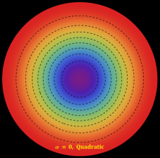
Refer to caption
Refer to caption
Refer to caption
Refer to caption
Refer to caption
Refer to caption
Refer to caption
Refer to caption
Figure 11: The flow of energyexchange𝑒𝑛𝑒𝑟𝑔𝑦𝑒𝑥𝑐𝑎𝑛𝑔𝑒energy-exchange between the fluid distributions for MIT Bag model by taking a=0𝑎0a=0 and g=60MeV/fm3subscript𝑔60𝑀𝑒𝑉𝑓superscript𝑚3\mathcal{B}_{g}=60\,MeV/fm^{3} (first two panels) and quadratic model by taking a=5\textkm2,b=1/3formulae-sequence𝑎5\text𝑘superscript𝑚2𝑏13a=5\,\text{km}^{2},~{}b=1/3 and g=60MeV/fm3subscript𝑔60𝑀𝑒𝑉𝑓superscript𝑚3\mathcal{B}_{g}=60\,MeV/fm^{3} (right two panels) with two different values of α𝛼\alpha for solution 3.1(ρ=θ00)\rho=\theta^{0}_{0})). The same values of constants are employed here as used in Fig.3.
Refer to caption
Refer to caption
Refer to caption
Refer to caption
Refer to caption
Refer to caption
Refer to caption
Refer to caption
Figure 12: The flow of energyexchange𝑒𝑛𝑒𝑟𝑔𝑦𝑒𝑥𝑐𝑎𝑛𝑔𝑒energy-exchange between the fluid distributions for MIT Bag model by taking a=0𝑎0a=0 and g=60MeV/fm3subscript𝑔60𝑀𝑒𝑉𝑓superscript𝑚3\mathcal{B}_{g}=60\,MeV/fm^{3} (first two panels) and quadratic model by taking a=2\textkm2,b=1/3formulae-sequence𝑎2\text𝑘superscript𝑚2𝑏13a=2\,\text{km}^{2},~{}b=1/3 and g=60MeV/fm3subscript𝑔60𝑀𝑒𝑉𝑓superscript𝑚3\mathcal{B}_{g}=60\,MeV/fm^{3} (right two panels) with two different values of α𝛼\alpha for solution 3.2(pr=θ11)p_{r}=\theta^{1}_{1})). The same values of constants are employed here as used in Fig.6.

6.0.2 For solution 3.2 (pr=θ11subscript𝑝𝑟subscriptsuperscript𝜃11p_{r}=\theta^{1}_{1})

This section contains the analysis of energy exchange (ΔEΔ𝐸\Delta E) distributions between the generic fluid θijsubscript𝜃𝑖𝑗\theta_{ij} and anisotropic fluid T^ijsubscript^𝑇𝑖𝑗\hat{T}_{ij} for solution 3.2. For this purpose, the density plot for Fig. 12 reveals the flow of energy between the relativistic fluids. The first two left figures are plotted in the context of the pure MIT bag model for decoupling constant α=0.1𝛼0.1\alpha=0.1 and α=0.2𝛼0.2\alpha=0.2, respectively using the bag constant value g=60MeV/fm3subscript𝑔60𝑀𝑒𝑉𝑓superscript𝑚3\mathcal{B}_{g}=60~{}MeV/fm^{3}. We observe that the ΔEΔ𝐸\Delta E is positive and minimum at the center while it starts increasing when moving towards the boundary but the maximum value of ΔEΔ𝐸\Delta E is achieved within the star, not at the boundary. On the other hand, we observe one interesting point here that no impact of the gravitational decoupling on the energy exchange fluid distributions is noticed under the mimic-to-pressures constraint approach. Therefore, the same maximum value of ΔE0.0005\textkm3Δ𝐸0.0005\text𝑘superscript𝑚3\Delta E\approx 0.0005~{}\text{km}^{-3} is observed for both values of α=0.1𝛼0.1\alpha=0.1 and 0.20.20.2. From the third and fourth panels, we show the distribution of energy for the quadratic model with decoupling constant values α=0.1𝛼0.1\alpha=0.1 and α=0.2𝛼0.2\alpha=0.2, respectively for the same value of bag constant g=60MeV/fm3subscript𝑔60𝑀𝑒𝑉𝑓superscript𝑚3\mathcal{B}_{g}=60~{}MeV/fm^{3}. We find that the behavior of energy exchange within the star for the quadratic model is similar to the MIT bag model but |ΔE|qua>|ΔE|MITsubscriptΔ𝐸𝑞𝑢𝑎subscriptΔ𝐸𝑀𝐼𝑇|\Delta E|_{qua}>|\Delta E|_{MIT} as happened in solution 3.1. The maximum value of ΔEΔ𝐸\Delta E is 0.00054\textkm30.00054\text𝑘superscript𝑚30.00054~{}\text{km}^{-3} at α=0.1𝛼0.1\alpha=0.1 and α=0.2𝛼0.2\alpha=0.2, both.

For the above solution, we finally can conclude that the interaction between both fluids also increases significantly when moving towards the boundary and reaches its maximum value within the star, not at the boundary, in all scenarios for the solution 3.2 (pr=θ11subscript𝑝𝑟subscriptsuperscript𝜃11p_{r}=\theta^{1}_{1}) as well as ΔEΔ𝐸\Delta E is positive throughout in the radial direction. Furthermore, the magnitude of the maximum value for ΔEΔ𝐸\Delta E is independent of decoupling constant α𝛼\alpha i.e. ΔEΔ𝐸\Delta E remains the same for each α𝛼\alpha. In fact here also, the generic source θijsubscript𝜃𝑖𝑗\theta_{ij} gives more energy to the environment in the presence of the quadratic EOS as compared to MIT bag model EOS.

Refer to caption
Refer to caption
Figure 13: Comparison of GR, GR+CGD, f(Q)𝑓𝑄f(Q) and f(Q)+limit-from𝑓𝑄f(Q)+CGD for both the solutions with the same value of constants employed as in Fig. 6.

7 Comparative study of model’s arising in GR, GR+CGD, f(𝒬)𝑓𝒬f(\mathcal{Q}) and f(𝒬)𝑓𝒬f(\mathcal{Q})+CGD gravity

In this section we highlight the key differences arising in general relativity (GR) and f(𝒬)𝑓𝒬f(\mathcal{Q}) gravity with and without CGD via our modeling framework. To this end, we draw the reader’s attention to Fig. 13. For the first case (ρ=θ00𝜌superscriptsubscript𝜃00\rho=\theta_{0}^{0}), we have plotted the M-R curves for pure GR  [β1=1,α=0formulae-sequencesubscript𝛽11𝛼0\beta_{1}=1,~{}\alpha=0] and pure f(𝒬)𝑓𝒬f(\mathcal{Q})  [β1=1.1,α=0formulae-sequencesubscript𝛽11.1𝛼0\beta_{1}=1.1,~{}\alpha=0] in Fig. 13 (top). We note that for the same EOS, the f(𝒬)limit-from𝑓𝒬f(\mathcal{Q})-gravity can generate higher Mmaxsubscript𝑀𝑚𝑎𝑥M_{max} than GR iff β1>1subscript𝛽11\beta_{1}>1, otherwise the reverse will happen. However, when CGD turns on i.e. α0𝛼0\alpha\neq 0, the corresponding EOS gets softer resulting in lower Mmaxsubscript𝑀𝑚𝑎𝑥M_{max} for both GR and f(𝒬)𝑓𝒬f(\mathcal{Q}) gravity. Therefore, when the ttlimit-from𝑡𝑡tt- component of the CGD-induced stress-tensor θijsuperscriptsubscript𝜃𝑖𝑗\theta_{i}^{j} mimics the density, the Mmaxsubscript𝑀𝑚𝑎𝑥M_{max} is lowered due to softening EOS. This can be ascribed to the effective density i.e. ϵ=(1+α)ρitalic-ϵ1𝛼𝜌\epsilon=(1+\alpha)\rho increasing with the CGD strength leading to a denser interior, which will eventually trigger many exotic processes such as hyperon and kaon productions. On the other hand, the second solution where θ11superscriptsubscript𝜃11\theta_{1}^{1} mimics pressure leads to the lowering of the effective pressure Pr=(1α)prsubscript𝑃𝑟1𝛼subscript𝑝𝑟P_{r}=(1-\alpha)p_{r}. In view of the EOS within the core, lower radial pressure supports lower interior density which may suppress any exotic phase transitions. This makes the EOS stiffer when the CGD strength increases leading to higher Mmaxsubscript𝑀𝑚𝑎𝑥M_{max} (see Fig. 13 bottom) and compactness parameter. Furthermore, it can also be observed that both f(𝒬)𝑓𝒬f(\mathcal{Q}) models yield roughly the same masses and radii when CGD is turned off. However, when CGD turns on the first case immediately decrease the Mmaxsubscript𝑀𝑚𝑎𝑥M_{max} and corresponding radius while the second solution yields a slightly higher maximum mass with smaller radius. In the GR limit, both solutions yield the same MR𝑀𝑅M-R curves as the seed solution is unaffected by β𝛽\beta.

8 Concluding Remarks and Astrophysical Implications

To make some concluding remarks on the present work and its outcomes, let us arrange the steps point-wise that what was our motivation and how we have carried out that in a successful way:

(i) Inspired by the recent gravitational event, i.e. GW190814 which brings to light the coalescence of a 23 Msubscript𝑀direct-productM_{\odot} black hole with a yet-to-be-determined secondary component, we try to model compact objects under the framework of f(𝒬)𝑓𝒬f(\mathcal{Q}) gravity theory along with the method of gravitational decoupling.

(ii) We assume a suitable quadratic equation of state (EOS) for the interior matter distribution of a compact star, especially a neutron/quark star, which in the appropriate limit reduces to the MIT bag model.

(iii) The concerned field equations under f(𝒬)𝑓𝒬f(\mathcal{Q}) gravity are subjected to gravitational decoupling bifurcates into the ρ=θ00𝜌subscriptsuperscript𝜃00\rho=\theta^{0}_{0} and pr=θ11subscript𝑝𝑟subscriptsuperscript𝜃11p_{r}=\theta^{1}_{1} sectors leading two distinct classes of solutions.

(iv) Both families of solutions are subjected to rigorous tests qualifying them to describe a class of compact stellar objects which include neutron stars, strange stars, and the possible progenitor of the secondary component of GW190814.

(v) Using observational data of mass-radius relations for compact objects, e.g. LMC X-4, Cen X-3, PSR J1614-2230, and PSR J0740+6620, we show that it is possible to generate stellar masses and radii beyond 2.5 Msubscript𝑀direct-productM_{\odot}.

(vi) The outcomes of the present work reveal that the quadratic EOS is versatile enough to account for a range of low-mass stars as well as typical stellar candidates describing the secondary component of GW190814.

Based on the above-mentioned steps, the obtained results have been already classified with detailed discussions in several tables and figures. Let us now put some salient features of the outcomes as follows:

1. Graphical plots for the basic physical parameters: Distribution of the energy density (Figs. 3 and 6), the radial pressure (Figs.3 and 6), and the anisotropy (Figs. 3 and 6) are exhibited for different values of the model parameters. Discussions in a length have been done already in 5.1.1 in connection to the solution 3.1 (ρ=θ00𝜌subscriptsuperscript𝜃00\rho=\theta^{0}_{0}) and in 5.1.2 in connection to the solution 3.2 (pr=θ11subscript𝑝𝑟subscriptsuperscript𝜃11p_{r}=\theta^{1}_{1}) respectively. We note that all the features are satisfactory as far as physical attributes are concerned.

2. Constraining upper limit of maximum mass via the graphical plots for M-R diagrams: For different choices of the linear EOS with constancy in bag constant, fixed decoupling parameter, and varying EOS parameter we have shown results in Tables 3-4 and figures 7-10 which are as follows.
In Table 3 and Fig. 7, we observe linear contributions from the energy density which do account for low-mass stars such as LMC X-4 and Cen X-3.
From Table 3 and Fig. 8 (left panel), we observe that an increase in the decoupling parameter results in a decrease in radii leading to more compact configurations. The left panel also shows that low mass stars such as LMC X-4 (1.29 ±plus-or-minus\pm 0.05 Msubscript𝑀direct-productM_{\odot}) and Cen X-3 (1.49 ±plus-or-minus\pm 0.08 Msubscript𝑀direct-productM_{\odot}) do exist for radii greater 10 km.

Figure 8 predicts a wide range of masses and radii applicable to observed compact objects, including the ’twin star’ scenario, the latter of which is favoured in the pr=θ11subscript𝑝𝑟subscriptsuperscript𝜃11p_{r}=\theta^{1}_{1} sector. Interestingly, the radii of these compact objects in f(R)𝑓𝑅f(R) gravity with rotation can vary between 12 to 18 km.
We ascertain from Table 4 and Fig. 10 that the quadratic EOS model fails to predict masses which can account for the LIGO observation of approximately 2.6 Msubscript𝑀direct-productM_{\odot} of the secondary component of the binary coalescence GW190814. It appears that when the linear and quadratic EOS parameters are switched on simultaneously, the decoupling constant quenches any increase in the mass of the compact object. While these models fail to predict masses above 2.6 Msubscript𝑀direct-productM_{\odot}, the quadratic EOS predicts the existence of well-known pulsars and neutron stars to a very good approximation. The tabulated data and plots reveal that the quadratic EOS which has the linear limit successfully predicts the existence of low-mass stars as well as neutron stars with masses beyond 2 Msubscript𝑀direct-productM_{\odot}.

3. Graphical plots for the energy exchange between the fluid distributions: We would now discuss The most important aspect of our findings, ie., the energy exchange arising from the extended gravitational decoupling. It is noted that temporal deformation is the same for both the solutions and hence the expressions of energy exchange will be the same for both cases but the amount of energy exchange will be different for both cases.
(i) For solution 3.1 (ρ=θ00𝜌subscriptsuperscript𝜃00\rho=\theta^{0}_{0}): In Fig. 11 we have exhibited the energy exchange between the relativistic fluids via the density plots. The first left figure is plotted in the context of the pure MIT bag model where we observe that the ΔEΔ𝐸\Delta E is positive and minimum at the center while starts increasing towards the boundary and attaining its maximum value within the star rather than the boundary. Now we move the second figure from the left which is plotted for the pure MIT bag model and one can note that the same situation occurs as happened before but the amount of energy exchange increases which is ΔEmax0.00058\textkm3Δsubscript𝐸𝑚𝑎𝑥0.00058\text𝑘superscript𝑚3\Delta E_{max}\approx 0.00058~{}\text{km}^{-3}.
The third and fourth panels show the distribution of energy for the quadratic model where the pattern of energy change within the star for the quadratic model is similar to the MIT bag model but |ΔE|qua>|ΔE|MITsubscriptΔ𝐸𝑞𝑢𝑎subscriptΔ𝐸𝑀𝐼𝑇|\Delta E|_{qua}>|\Delta E|_{MIT}. The maximum value of ΔEΔ𝐸\Delta E is 0.00063\textkm30.00063\text𝑘superscript𝑚30.00063~{}\text{km}^{-3} and 0.00067\textkm30.00067\text𝑘superscript𝑚30.00067~{}\text{km}^{-3} at α=0.1𝛼0.1\alpha=0.1 and α=0.2𝛼0.2\alpha=0.2, respectively.

Based on the above observations, one may conclude that the interaction between both fluids increases significantly when moving towards the boundary and reaches its maximum value within the star, not at the boundary in all cases for the solution 3.1 (ρ=θ00𝜌subscriptsuperscript𝜃00\rho=\theta^{0}_{0}). Also, ΔEΔ𝐸\Delta E is positive throughout in the radial direction as well as its magnitude of maximum value increases when the decoupling constant α𝛼\alpha increases. Furthermore, the generic source θijsubscript𝜃𝑖𝑗\theta_{ij} gives more energy to the environment in the presence of the quadratic EOS as compared to MIT bag model EOS.
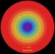
(ii) For solution 3.2 (pr=θ11subscript𝑝𝑟subscriptsuperscript𝜃11p_{r}=\theta^{1}_{1}): The density plot for Fig. 12 has been shown to observe the flow of energy exchange between the relativistic fluids. The first two left figures are plotted in the context of the pure MIT bag model where we observe that the ΔEΔ𝐸\Delta E is positive and minimum at the center while it starts increasing when moving towards the boundary but the maximum value of ΔEΔ𝐸\Delta E is achieved within the star, not at the boundary. On the other hand, we observe one interesting point here that no impact of the gravitational decoupling on the energy exchange fluid distributions is noticed under the mimic-to-pressures constraint approach. From the third and fourth panels, we show the distribution of energy for the quadratic model and find that the behavior of energy exchange within the star for the quadratic model is similar to the MIT bag model but |ΔE|qua>|ΔE|MITsubscriptΔ𝐸𝑞𝑢𝑎subscriptΔ𝐸𝑀𝐼𝑇|\Delta E|_{qua}>|\Delta E|_{MIT} as happened in solution 3.1.

Therefore, we can conclude that the interaction between both fluids also increases significantly when moving towards the boundary and reaches its maximum value within the star, not at the boundary in all the situations for the solution 3.2 (pr=θ11subscript𝑝𝑟subscriptsuperscript𝜃11p_{r}=\theta^{1}_{1}) as well as ΔEΔ𝐸\Delta E is positive throughout in the radial direction. Furthermore, the magnitude of the maximum value for ΔEΔ𝐸\Delta E is independent of decoupling constant α𝛼\alpha, i.e. ΔEΔ𝐸\Delta E remains the same for each α𝛼\alpha. In fact here also, the generic source θijsubscript𝜃𝑖𝑗\theta_{ij} gives more energy to the environment in the presence of the quadratic EOS as compared to MIT bag model EOS.

The overall findings of the models presented reveal that it is possible to put suitable constraints on the upper limit of the mass-radius relation of the secondary component of GW190814 and other self-bound strange star configurations under gravitational decoupling in f(𝒬)𝑓𝒬f(\mathcal{Q})-gravity theory which may provide the observational signature of the objects in a significant way.

Acknowledgement

The author SKM is thankful for continuous support and encouragement from the administration of the University of Nizwa to carry out the research work. G. Mustafa is very thankful to Prof. Gao Xianlong from the Department of Physics, Zhejiang Normal University, for his kind support and help during this research. Further, G. Mustafa acknowledges Grant No. ZC304022919 to support his Postdoctoral Fellowship at Zhejiang Normal University. KNS and SR are also thankful to the authorities of the Inter-University Centre for Astronomy and Astrophysics, Pune, India for providing the research facilities where SR specifically expresses thanks to ICARD of IUCAA at GLA University. The authors are also thankful to Prof. Jorge Ovalle for his help in the coding of the contour diagrams.

DATA AVAILABILITY:

No new data were generated or analyzed in support of this research.

Appendix

θ11(r)=14[1β1L(LN)(Lr2+1)(4β1L3(13aβ2\displaystyle\theta_{11}(r)=\frac{1}{4}\Bigg{[}\frac{1}{\beta_{1}L(L-N)\left(Lr^{2}+1\right)}\Big{(}-4\beta_{1}L^{3}(1-3a\beta_{2}
+6aβ1N+3b)+L2(β2(aβ22b2)8β1N(2aβ2\displaystyle\hskip 17.07182pt+6a\beta_{1}N+3b)+L^{2}\big{(}\beta_{2}(a\beta_{2}-2b-2)-8\beta_{1}N(2a\beta_{2}
2b1)+4aβ12N2)2LN(β2(aβ22b2)+2β1\displaystyle\hskip 17.07182pt-2b-1)+4a\beta_{1}^{2}N^{2}\big{)}-2LN(\beta_{2}(a\beta_{2}-2b-2)+2\beta_{1}
×N(aβ2+b+1))+β2N2(aβ22b2)+36aβ12\displaystyle\hskip 17.07182pt\times N(-a\beta_{2}+b+1))+\beta_{2}N^{2}(a\beta_{2}-2b-2)+36a\beta_{1}^{2}
×L4+4c(LN)2)+N(β2(aβ22b2)+4c)β1L\displaystyle\hskip 17.07182pt\times L^{4}+4c(L-N)^{2}\Big{)}+\frac{N(\beta_{2}(a\beta_{2}-2b-2)+4c)}{\beta_{1}L}
+4N(a(9β1L2+2β2L6β1LN+β1N22β2N))(NL)(Nr2+1)4𝑁𝑎9subscript𝛽1superscript𝐿22subscript𝛽2𝐿6subscript𝛽1𝐿𝑁subscript𝛽1superscript𝑁22subscript𝛽2𝑁𝑁𝐿𝑁superscript𝑟21\displaystyle\hskip 17.07182pt+\frac{4N\big{(}a\big{(}9\beta_{1}L^{2}+2\beta_{2}L-6\beta_{1}LN+\beta_{1}N^{2}-2\beta_{2}N\big{)}\big{)}}{(N-L)\big{(}Nr^{2}+1\big{)}}
16aβ1N(2LN)2b(Nr2+1)(Nr2+1)216aβ1N(LN)(Nr2+1)3],\displaystyle\hskip 17.07182pt-\frac{16a\beta_{1}N(2L-N)-2b(Nr^{2}+1)}{\big{(}Nr^{2}+1\big{)}^{2}}-\frac{16a\beta_{1}N(L-N)}{\big{(}Nr^{2}+1\big{)}^{3}}\Bigg{]},\,
θ22(r)=14β1(Lr2+1)2(Nr2+1)4[aβ224β1L2\displaystyle\theta_{22}(r)=-\frac{1}{4\beta_{1}\big{(}Lr^{2}+1\big{)}^{2}\big{(}Nr^{2}+1\big{)}^{4}}\Big{[}-a\beta_{2}^{2}-4\beta_{1}L^{2}
×(9aβ1+N4r10(1aβ2+b)+2N3r8(5aβ2\displaystyle\hskip 17.07182pt\times\big{(}9a\beta_{1}+N^{4}r^{10}(1-a\beta_{2}+b)+2N^{3}r^{8}(-5a\beta_{2}
+3aβ1N+5b+2)+N2r6(20aβ2+53aβ1N+20b\displaystyle\hskip 17.07182pt+3a\beta_{1}N+5b+2)+N^{2}r^{6}(-20a\beta_{2}+53a\beta_{1}N+20b
+6)+Nr4(14aβ2+101aβ1N+14b+4)+r2(3a\displaystyle\hskip 17.07182pt+6)+Nr^{4}(-14a\beta_{2}+101a\beta_{1}N+14b+4)+r^{2}(-3a
×(β2+3β1N)+3b+1))+L{4β1(Nr2+1)2[3aβ2\displaystyle\hskip 17.07182pt\times(\beta_{2}+3\beta_{1}N)+3b+1)\big{)}+L\big{\{}4\beta_{1}\big{(}Nr^{2}+1\big{)}^{2}\big{[}-3a\beta_{2}
+N3r6(1aβ2)+3N2r4(13aβ2)3Nr2(aβ21)superscript𝑁3superscript𝑟61𝑎subscript𝛽23superscript𝑁2superscript𝑟413𝑎subscript𝛽23𝑁superscript𝑟2𝑎subscript𝛽21\displaystyle\hskip 17.07182pt+N^{3}r^{6}(1-a\beta_{2})+3N^{2}r^{4}(1-3a\beta_{2})-3Nr^{2}(a\beta_{2}-1)
+b(N3r6+9N2r4+3Nr2+3)+1]+β2r2(Nr21)\displaystyle\hskip 17.07182pt+b\big{(}N^{3}r^{6}+9N^{2}r^{4}+3Nr^{2}+3\big{)}+1\big{]}+\beta_{2}r^{2}\big{(}Nr^{2}-1\big{)}
×(Nr2+1)4(aβ2+2b+2)+4aβ12N(3N4r8+25N3\displaystyle\hskip 14.22636pt\times\big{(}Nr^{2}+1\big{)}^{4}(-a\beta_{2}+2b+2)+4a\beta_{1}^{2}N\big{(}3N^{4}r^{8}+25N^{3}
×r6+31N2r445Nr2+18)}+12aβ12L3r2(N3r6\displaystyle\hskip 17.07182pt\times r^{6}+31N^{2}r^{4}-45Nr^{2}+18\big{)}\big{\}}+12a\beta_{1}^{2}L^{3}r^{2}\big{(}N^{3}r^{6}
+9N2r4+19Nr2+3)3aβ22N5r10+4aβ1β2N5r8\displaystyle\hskip 17.07182pt+9N^{2}r^{4}+19Nr^{2}+3\big{)}-3a\beta_{2}^{2}N^{5}r^{10}+4a\beta_{1}\beta_{2}N^{5}r^{8}
+4aβ12N5r613aβ22N4r8+8aβ1β2N4r6+52aβ124𝑎superscriptsubscript𝛽12superscript𝑁5superscript𝑟613𝑎superscriptsubscript𝛽22superscript𝑁4superscript𝑟88𝑎subscript𝛽1subscript𝛽2superscript𝑁4superscript𝑟652𝑎superscriptsubscript𝛽12\displaystyle\hskip 17.07182pt+4a\beta_{1}^{2}N^{5}r^{6}-13a\beta_{2}^{2}N^{4}r^{8}+8a\beta_{1}\beta_{2}N^{4}r^{6}+52a\beta_{1}^{2}
×N4r422aβ22N3r6+16aβ1β2N3r4+108aβ12N3r2absentsuperscript𝑁4superscript𝑟422𝑎superscriptsubscript𝛽22superscript𝑁3superscript𝑟616𝑎subscript𝛽1subscript𝛽2superscript𝑁3superscript𝑟4108𝑎superscriptsubscript𝛽12superscript𝑁3superscript𝑟2\displaystyle\hskip 17.07182pt\times N^{4}r^{4}-22a\beta_{2}^{2}N^{3}r^{6}+16a\beta_{1}\beta_{2}N^{3}r^{4}+108a\beta_{1}^{2}N^{3}r^{2}
36aβ12N218aβ22N2r4+24aβ1β2N2r2+12aβ1β2N36𝑎superscriptsubscript𝛽12superscript𝑁218𝑎superscriptsubscript𝛽22superscript𝑁2superscript𝑟424𝑎subscript𝛽1subscript𝛽2superscript𝑁2superscript𝑟212𝑎subscript𝛽1subscript𝛽2𝑁\displaystyle\hskip 17.07182pt-36a\beta_{1}^{2}N^{2}-18a\beta_{2}^{2}N^{2}r^{4}+24a\beta_{1}\beta_{2}N^{2}r^{2}+12a\beta_{1}\beta_{2}N
7aβ22Nr2+2bβ2+6bβ2N5r104β1bN5r8+26bβ2N47𝑎superscriptsubscript𝛽22𝑁superscript𝑟22𝑏subscript𝛽26𝑏subscript𝛽2superscript𝑁5superscript𝑟104subscript𝛽1𝑏superscript𝑁5superscript𝑟826𝑏subscript𝛽2superscript𝑁4\displaystyle\hskip 17.07182pt-7a\beta_{2}^{2}Nr^{2}+2b\beta_{2}+6b\beta_{2}N^{5}r^{10}-4\beta_{1}bN^{5}r^{8}+26b\beta_{2}N^{4}
×r88β1bN4r6+44bβ2N3r616β1bN3r4+36bβ2absentsuperscript𝑟88subscript𝛽1𝑏superscript𝑁4superscript𝑟644𝑏subscript𝛽2superscript𝑁3superscript𝑟616subscript𝛽1𝑏superscript𝑁3superscript𝑟436𝑏subscript𝛽2\displaystyle\hskip 17.07182pt\times r^{8}-8\beta_{1}bN^{4}r^{6}+44b\beta_{2}N^{3}r^{6}-16\beta_{1}bN^{3}r^{4}+36b\beta_{2}
×N2r424β1bN2r212β1bN+14bβ2Nr2+2β24cabsentsuperscript𝑁2superscript𝑟424subscript𝛽1𝑏superscript𝑁2superscript𝑟212subscript𝛽1𝑏𝑁14𝑏subscript𝛽2𝑁superscript𝑟22subscript𝛽24𝑐\displaystyle\hskip 17.07182pt\times N^{2}r^{4}-24\beta_{1}bN^{2}r^{2}-12\beta_{1}bN+14b\beta_{2}Nr^{2}+2\beta_{2}-4c
×(Nr2+1)4(Lr2(Nr21)+3Nr2+1)+6β2N5r10absentsuperscript𝑁superscript𝑟214𝐿superscript𝑟2𝑁superscript𝑟213𝑁superscript𝑟216subscript𝛽2superscript𝑁5superscript𝑟10\displaystyle\hskip 17.07182pt\times\big{(}Nr^{2}+1\big{)}^{4}\big{(}Lr^{2}\big{(}Nr^{2}-1\big{)}+3Nr^{2}+1\big{)}+6\beta_{2}N^{5}r^{10}
4β1N5r8+26β2N4r816β1N4r6+44β2N3r624β14subscript𝛽1superscript𝑁5superscript𝑟826subscript𝛽2superscript𝑁4superscript𝑟816subscript𝛽1superscript𝑁4superscript𝑟644subscript𝛽2superscript𝑁3superscript𝑟624subscript𝛽1\displaystyle\hskip 17.07182pt-4\beta_{1}N^{5}r^{8}+26\beta_{2}N^{4}r^{8}-16\beta_{1}N^{4}r^{6}+44\beta_{2}N^{3}r^{6}-24\beta_{1}
×N3r4+36β2N2r416β1N2r24β1N+14β2Nr2].\displaystyle\hskip 17.07182pt\times N^{3}r^{4}+36\beta_{2}N^{2}r^{4}-16\beta_{1}N^{2}r^{2}-4\beta_{1}N+14\beta_{2}Nr^{2}\Big{]}.
θ23(r)=θ112(r)r2(Nr2+1)[6β1{kLr2+k+(α2+2α+3)\displaystyle\theta_{23}(r)=\theta^{2}_{11}(r)r^{2}\left(Nr^{2}+1\right)\big{[}6\beta_{1}\big{\{}kLr^{2}+k+\big{(}\alpha^{2}+2\alpha+3\big{)}
×Lr2α2Nr22αNr2Nr2+2}+(α+1)2β2r2\displaystyle\hskip 17.07182pt\times Lr^{2}-\alpha^{2}Nr^{2}-2\alpha Nr^{2}-Nr^{2}+2\big{\}}+(\alpha+1)^{2}\beta_{2}r^{2}
×(Nr2+1)]+4θ11(r)(3β1((α+2)Lr2(Nr2+2)\displaystyle\hskip 17.07182pt\times\left(Nr^{2}+1\right)\big{]}+4\theta_{11}(r)\big{(}3\beta_{1}\big{(}(\alpha+2)Lr^{2}\left(Nr^{2}+2\right)
(α+1)N2r42(α+1)Nr2+1)+(α+1)β2\displaystyle\hskip 17.07182pt-(\alpha+1)-N^{2}r^{4}-2(\alpha+1)Nr^{2}+1\big{)}+(\alpha+1)\beta_{2}
×(Nr3+r)2)+4(β2+6β1L+β2N2r46β1N\displaystyle\hskip 17.07182pt\times\left(Nr^{3}+r\right)^{2}\big{)}+4\big{(}\beta_{2}+6\beta_{1}L+\beta_{2}N^{2}r^{4}-6\beta_{1}N
+2β2Nr2),\displaystyle\hskip 17.07182pt+2\beta_{2}Nr^{2}\big{)},
Ψ21(r)=4β1(Nr2+1)2[Nr2(α3αaβ2+αLr2(aβ21)\displaystyle\Psi_{21}(r)=4\beta_{1}\big{(}Nr^{2}+1\big{)}^{2}\big{[}Nr^{2}\big{(}\alpha-3\alpha a\beta_{2}+\alpha Lr^{2}(a\beta_{2}-1)
+aβ2(Lr23)+2)+3αaβ2Lr2+3aβ2Lr2(α+1)N2r4\displaystyle\hskip 8.5359pt+a\beta_{2}\big{(}Lr^{2}-3\big{)}+2\big{)}+3\alpha a\beta_{2}Lr^{2}+3a\beta_{2}Lr^{2}-(\alpha+1)N^{2}r^{4}
×(aβ21)(α+1)br2(LN)(Nr2+3)αLr2+1]\displaystyle\hskip 8.5359pt\times(a\beta_{2}-1)-(\alpha+1)br^{2}(L-N)\big{(}Nr^{2}+3\big{)}-\alpha Lr^{2}+1\big{]}
+(α+1)β2r2(Nr2+1)4(aβ22b2)+4(α+1)aβ12r2𝛼1subscript𝛽2superscript𝑟2superscript𝑁superscript𝑟214𝑎subscript𝛽22𝑏24𝛼1𝑎superscriptsubscript𝛽12superscript𝑟2\displaystyle\hskip 8.5359pt+(\alpha+1)\beta_{2}r^{2}\big{(}Nr^{2}+1\big{)}^{4}(a\beta_{2}-2b-2)+4(\alpha+1)a\beta_{1}^{2}r^{2}
×(LN)2(Nr2+3)2+4(α+1)cr2(Nr2+1)4,absentsuperscript𝐿𝑁2superscript𝑁superscript𝑟2324𝛼1𝑐superscript𝑟2superscript𝑁superscript𝑟214\displaystyle\hskip 8.5359pt\times(L-N)^{2}\big{(}Nr^{2}+3\big{)}^{2}+4(\alpha+1)cr^{2}\big{(}Nr^{2}+1\big{)}^{4},
Ψ22(r)=+N(36aβ1+r2(314aβ2))+2b(Nr2+1)2(Nr2\displaystyle\Psi_{22}(r)=+N\big{(}36a\beta_{1}+r^{2}(3-14a\beta_{2})\big{)}+2b\big{(}Nr^{2}+1\big{)}^{2}\big{(}Nr^{2}
+3)+1]+4aβ12L2(Nr2+3)2+aβ22N4r84aβ1β2N4r6\displaystyle\hskip 5.69046pt+3\big{)}+1\big{]}+4a\beta_{1}^{2}L^{2}\big{(}Nr^{2}+3\big{)}^{2}+a\beta_{2}^{2}N^{4}r^{8}-4a\beta_{1}\beta_{2}N^{4}r^{6}
+4aβ12N4r4+4aβ22N3r620aβ1β2N3r4+24aβ12N3r24𝑎superscriptsubscript𝛽12superscript𝑁4superscript𝑟44𝑎superscriptsubscript𝛽22superscript𝑁3superscript𝑟620𝑎subscript𝛽1subscript𝛽2superscript𝑁3superscript𝑟424𝑎superscriptsubscript𝛽12superscript𝑁3superscript𝑟2\displaystyle\hskip 5.69046pt+4a\beta_{1}^{2}N^{4}r^{4}\ +4a\beta_{2}^{2}N^{3}r^{6}-20a\beta_{1}\beta_{2}N^{3}r^{4}+24a\beta_{1}^{2}N^{3}r^{2}
+36aβ12N2+6aβ22N2r428aβ1β2N2r212aβ1β2N36𝑎superscriptsubscript𝛽12superscript𝑁26𝑎superscriptsubscript𝛽22superscript𝑁2superscript𝑟428𝑎subscript𝛽1subscript𝛽2superscript𝑁2superscript𝑟212𝑎subscript𝛽1subscript𝛽2𝑁\displaystyle\hskip 5.69046pt+36a\beta_{1}^{2}N^{2}+6a\beta_{2}^{2}N^{2}r^{4}-28a\beta_{1}\beta_{2}N^{2}r^{2}-12a\beta_{1}\beta_{2}N
+4aβ22Nr22bβ22bβ2N4r8+4β1bN4r68bβ2N3r64𝑎superscriptsubscript𝛽22𝑁superscript𝑟22𝑏subscript𝛽22𝑏subscript𝛽2superscript𝑁4superscript𝑟84subscript𝛽1𝑏superscript𝑁4superscript𝑟68𝑏subscript𝛽2superscript𝑁3superscript𝑟6\displaystyle\hskip 5.69046pt+4a\beta_{2}^{2}Nr^{2}-2b\beta_{2}-2b\beta_{2}N^{4}r^{8}+4\beta_{1}bN^{4}r^{6}-8b\beta_{2}N^{3}r^{6}
+20β1bN3r412bβ2N2r4+28β1bN2r2+12β1bN8bβ220subscript𝛽1𝑏superscript𝑁3superscript𝑟412𝑏subscript𝛽2superscript𝑁2superscript𝑟428subscript𝛽1𝑏superscript𝑁2superscript𝑟212subscript𝛽1𝑏𝑁8𝑏subscript𝛽2\displaystyle\hskip 5.69046pt+20\beta_{1}bN^{3}r^{4}-12b\beta_{2}N^{2}r^{4}+28\beta_{1}bN^{2}r^{2}+12\beta_{1}bN-8b\beta_{2}
×Nr2β2+4c(Nr2+1)4β2N3r6(1+4Nr2)+2β1N4r6absent𝑁superscript𝑟2subscript𝛽24𝑐superscript𝑁superscript𝑟214subscript𝛽2superscript𝑁3superscript𝑟614𝑁superscript𝑟22subscript𝛽1superscript𝑁4superscript𝑟6\displaystyle\hskip 5.69046pt\times Nr^{2}-\beta_{2}+4c\big{(}Nr^{2}+1\big{)}^{4}-\beta_{2}N^{3}r^{6}(1+4Nr^{2})+2\beta_{1}N^{4}r^{6}
+6β1N3r46β2N2r4+6β1N2r2+2β1N4β2Nr2,6subscript𝛽1superscript𝑁3superscript𝑟46subscript𝛽2superscript𝑁2superscript𝑟46subscript𝛽1superscript𝑁2superscript𝑟22subscript𝛽1𝑁4subscript𝛽2𝑁superscript𝑟2\displaystyle\hskip 5.69046pt+6\beta_{1}N^{3}r^{4}-6\beta_{2}N^{2}r^{4}+6\beta_{1}N^{2}r^{2}+2\beta_{1}N-4\beta_{2}Nr^{2},
Ψ00(r)=[2aβ22β1L(N2(r4(36aβ2)+8aβ1r2)14aβ2\displaystyle\Psi_{00}(r)=\big{[}2a\beta_{2}^{2}-\beta_{1}L\big{(}N^{2}\big{(}r^{4}(3-6a\beta_{2})+8a\beta_{1}r^{2}\big{)}-14a\beta_{2}
+N(24aβ1+r2(620aβ2))+2b(3N2r4+10Nr2+7)𝑁24𝑎subscript𝛽1superscript𝑟2620𝑎subscript𝛽22𝑏3superscript𝑁2superscript𝑟410𝑁superscript𝑟27\displaystyle\hskip 8.5359pt+N\big{(}24a\beta_{1}+r^{2}(6-20a\beta_{2})\big{)}+2b\big{(}3N^{2}r^{4}+10Nr^{2}+7\big{)}
+3)+4aβ12L2(Nr2+3)+2aN3(β22r63β1β2r4+2β12r2)\displaystyle\hskip 8.5359pt+3\big{)}+4a\beta_{1}^{2}L^{2}\big{(}Nr^{2}+3\big{)}+2aN^{3}(\beta_{2}^{2}r^{6}-3\beta_{1}\beta_{2}r^{4}+2\beta_{1}^{2}r^{2})
+12aβ12N2+6aβ22N2r420aβ1β2N2r214aβ1β2N12𝑎superscriptsubscript𝛽12superscript𝑁26𝑎superscriptsubscript𝛽22superscript𝑁2superscript𝑟420𝑎subscript𝛽1subscript𝛽2superscript𝑁2superscript𝑟214𝑎subscript𝛽1subscript𝛽2𝑁\displaystyle\hskip 8.5359pt+12a\beta_{1}^{2}N^{2}+6a\beta_{2}^{2}N^{2}r^{4}-20a\beta_{1}\beta_{2}N^{2}r^{2}-14a\beta_{1}\beta_{2}N
+6aβ22Nr24bβ24bβ2N3r6+6β1bN3r412bβ2N2r46𝑎superscriptsubscript𝛽22𝑁superscript𝑟24𝑏subscript𝛽24𝑏subscript𝛽2superscript𝑁3superscript𝑟66subscript𝛽1𝑏superscript𝑁3superscript𝑟412𝑏subscript𝛽2superscript𝑁2superscript𝑟4\displaystyle\hskip 8.5359pt+6a\beta_{2}^{2}Nr^{2}-4b\beta_{2}-4b\beta_{2}N^{3}r^{6}+6\beta_{1}bN^{3}r^{4}-12b\beta_{2}N^{2}r^{4}
+20β1bN2r2+14β1bN12bβ2Nr22β2+8c(Nr2+1)320subscript𝛽1𝑏superscript𝑁2superscript𝑟214subscript𝛽1𝑏𝑁12𝑏subscript𝛽2𝑁superscript𝑟22subscript𝛽28𝑐superscript𝑁superscript𝑟213\displaystyle\hskip 8.5359pt+20\beta_{1}bN^{2}r^{2}+14\beta_{1}bN-12b\beta_{2}Nr^{2}-2\beta_{2}+8c\big{(}Nr^{2}+1\big{)}^{3}
2β2N3r6+3β1N3r46β2N2r4+6β1N2r2+3β1N6β22subscript𝛽2superscript𝑁3superscript𝑟63subscript𝛽1superscript𝑁3superscript𝑟46subscript𝛽2superscript𝑁2superscript𝑟46subscript𝛽1superscript𝑁2superscript𝑟23subscript𝛽1𝑁6subscript𝛽2\displaystyle\hskip 8.5359pt-2\beta_{2}N^{3}r^{6}+3\beta_{1}N^{3}r^{4}-6\beta_{2}N^{2}r^{4}+6\beta_{1}N^{2}r^{2}+3\beta_{1}N-6\beta_{2}
×Nr2][4β1(Nr2+1)2(Nr2(α3αaβ2+αLr2(aβ21)\displaystyle\hskip 8.5359pt\times Nr^{2}\big{]}\big{[}4\beta_{1}\big{(}Nr^{2}+1\big{)}^{2}\big{(}Nr^{2}\big{(}\alpha-3\alpha a\beta_{2}+\alpha Lr^{2}(a\beta_{2}-1)
+aβ2(Lr23)+2)+3αaβ2Lr2+3aβ2Lr2(α+1)Nr4\displaystyle\hskip 8.5359pt+a\beta_{2}\big{(}Lr^{2}-3\big{)}+2\big{)}+3\alpha a\beta_{2}Lr^{2}+3a\beta_{2}Lr^{2}-(\alpha+1)Nr^{4}
×(aβ21)(α+1)br2(LN)(Nr2+3)αLr2+1)\displaystyle\hskip 8.5359pt\times(a\beta_{2}-1)-(\alpha+1)br^{2}(L-N)\big{(}Nr^{2}+3\big{)}-\alpha Lr^{2}+1\big{)}
+(α+1)β2r2(Nr2+1)4(aβ22b2)+4(α+1)aβ12r2𝛼1subscript𝛽2superscript𝑟2superscript𝑁superscript𝑟214𝑎subscript𝛽22𝑏24𝛼1𝑎superscriptsubscript𝛽12superscript𝑟2\displaystyle\hskip 8.5359pt+(\alpha+1)\beta_{2}r^{2}\big{(}Nr^{2}+1\big{)}^{4}(a\beta_{2}-2b-2)+4(\alpha+1)a\beta_{1}^{2}r^{2}
×(LN)2(Nr2+3)2+4(α+1)cr2(Nr2+1)4]\displaystyle\hskip 8.5359pt\times(L-N)^{2}\big{(}Nr^{2}+3\big{)}^{2}+4(\alpha+1)cr^{2}\big{(}Nr^{2}+1\big{)}^{4}\big{]}
f1(r)=1(Nr2+1)3(β1+β1Lr2)[aβ224β1L(3aβ2+N3\displaystyle f_{1}(r)=\frac{1}{\left(Nr^{2}+1\right)^{3}\left(\beta_{1}+\beta_{1}Lr^{2}\right)}\Big{[}a\beta_{2}^{2}-4\beta_{1}L\big{(}-3a\beta_{2}+N^{3}
×(r6(1aβ2)+2aβ1r4)+N2(r4(35aβ2)+12aβ1r2)absentsuperscript𝑟61𝑎subscript𝛽22𝑎subscript𝛽1superscript𝑟4superscript𝑁2superscript𝑟435𝑎subscript𝛽212𝑎subscript𝛽1superscript𝑟2\displaystyle\hskip 5.69046pt\times\big{(}r^{6}(1-a\beta_{2})+2a\beta_{1}r^{4}\big{)}+N^{2}\big{(}r^{4}(3-5a\beta_{2})+12a\beta_{1}r^{2}\big{)}
+N(18aβ1+r2(37aβ2))+b(Nr2+1)2(Nr2+3)+1)\displaystyle\hskip 5.69046pt+N\big{(}18a\beta_{1}+r^{2}(3-7a\beta_{2})\big{)}+b\big{(}Nr^{2}+1\big{)}^{2}\big{(}Nr^{2}+3\big{)}+1\big{)}
+4aβ12L2(Nr2+3)2+aβ22N4r84aβ1β2N4r6+4aβ12N4r44𝑎superscriptsubscript𝛽12superscript𝐿2superscript𝑁superscript𝑟232𝑎superscriptsubscript𝛽22superscript𝑁4superscript𝑟84𝑎subscript𝛽1subscript𝛽2superscript𝑁4superscript𝑟64𝑎superscriptsubscript𝛽12superscript𝑁4superscript𝑟4\displaystyle\hskip 5.69046pt+4a\beta_{1}^{2}L^{2}\big{(}Nr^{2}+3\big{)}^{2}+a\beta_{2}^{2}N^{4}r^{8}-4a\beta_{1}\beta_{2}N^{4}r^{6}+4a\beta_{1}^{2}N^{4}r^{4}
+4aβ22N3r620aβ1β2N3r4+24aβ12N3r2+36aβ12N24𝑎superscriptsubscript𝛽22superscript𝑁3superscript𝑟620𝑎subscript𝛽1subscript𝛽2superscript𝑁3superscript𝑟424𝑎superscriptsubscript𝛽12superscript𝑁3superscript𝑟236𝑎superscriptsubscript𝛽12superscript𝑁2\displaystyle\hskip 5.69046pt+4a\beta_{2}^{2}N^{3}r^{6}-20a\beta_{1}\beta_{2}N^{3}r^{4}+24a\beta_{1}^{2}N^{3}r^{2}+36a\beta_{1}^{2}N^{2}
+6aβ22N2r428aβ1β2N2r212aβ1β2N+4aβ22Nr22bβ26𝑎superscriptsubscript𝛽22superscript𝑁2superscript𝑟428𝑎subscript𝛽1subscript𝛽2superscript𝑁2superscript𝑟212𝑎subscript𝛽1subscript𝛽2𝑁4𝑎superscriptsubscript𝛽22𝑁superscript𝑟22𝑏subscript𝛽2\displaystyle\hskip 5.69046pt+6a\beta_{2}^{2}N^{2}r^{4}-28a\beta_{1}\beta_{2}N^{2}r^{2}-12a\beta_{1}\beta_{2}N+4a\beta_{2}^{2}Nr^{2}-2b\beta_{2}
2bβ2N4r8+4β1bN4r68bβ2N3r6+20β1bN3r412bβ22𝑏subscript𝛽2superscript𝑁4superscript𝑟84subscript𝛽1𝑏superscript𝑁4superscript𝑟68𝑏subscript𝛽2superscript𝑁3superscript𝑟620subscript𝛽1𝑏superscript𝑁3superscript𝑟412𝑏subscript𝛽2\displaystyle\hskip 5.69046pt-2b\beta_{2}N^{4}r^{8}+4\beta_{1}bN^{4}r^{6}-8b\beta_{2}N^{3}r^{6}+20\beta_{1}bN^{3}r^{4}-12b\beta_{2}
×N2r4+28β1bN2r2+12β1bN8bβ2Nr22β2+4babsentsuperscript𝑁2superscript𝑟428subscript𝛽1𝑏superscript𝑁2superscript𝑟212subscript𝛽1𝑏𝑁8𝑏subscript𝛽2𝑁superscript𝑟22subscript𝛽24𝑏\displaystyle\hskip 5.69046pt\times N^{2}r^{4}+28\beta_{1}bN^{2}r^{2}+12\beta_{1}bN-8b\beta_{2}Nr^{2}-2\beta_{2}+4b
×(Nr2+1)42β2N4r8+4β1N4r68β2N3r6+12β1N3r4absentsuperscript𝑁superscript𝑟2142subscript𝛽2superscript𝑁4superscript𝑟84subscript𝛽1superscript𝑁4superscript𝑟68subscript𝛽2superscript𝑁3superscript𝑟612subscript𝛽1superscript𝑁3superscript𝑟4\displaystyle\hskip 5.69046pt\times\big{(}Nr^{2}+1\big{)}^{4}-2\beta_{2}N^{4}r^{8}+4\beta_{1}N^{4}r^{6}-8\beta_{2}N^{3}r^{6}+12\beta_{1}N^{3}r^{4}
12β2N2r4+12β1N2r212subscript𝛽2superscript𝑁2superscript𝑟412subscript𝛽1superscript𝑁2superscript𝑟2\displaystyle\hskip 5.69046pt-12\beta_{2}N^{2}r^{4}+12\beta_{1}N^{2}r^{2}
+4β1N8β2Nr2],\displaystyle\hskip 5.69046pt+4\beta_{1}N-8\beta_{2}Nr^{2}\Big{]},
f2(r)=2[{(NL)(aN4β22r82bN4β2r82N4β2r8+4aN3\displaystyle f_{2}(r)=2\Big{[}\Big{\{}(N-L)\Big{(}aN^{4}\beta_{2}^{2}r^{8}-2bN^{4}\beta_{2}r^{8}-2N^{4}\beta_{2}r^{8}+4aN^{3}
×β22r68bN3β2r68N3β2r64aN4β12r4+6aN2β22r4absentsuperscriptsubscript𝛽22superscript𝑟68𝑏superscript𝑁3subscript𝛽2superscript𝑟68superscript𝑁3subscript𝛽2superscript𝑟64𝑎superscript𝑁4superscriptsubscript𝛽12superscript𝑟46𝑎superscript𝑁2superscriptsubscript𝛽22superscript𝑟4\displaystyle\hskip 5.69046pt\times\beta_{2}^{2}r^{6}-8bN^{3}\beta_{2}r^{6}-8N^{3}\beta_{2}r^{6}-4aN^{4}\beta_{1}^{2}r^{4}+6aN^{2}\beta_{2}^{2}r^{4}
8bN3β1r412bN2β2r412N2β2r4+8aN3β1β2r440a8𝑏superscript𝑁3subscript𝛽1superscript𝑟412𝑏superscript𝑁2subscript𝛽2superscript𝑟412superscript𝑁2subscript𝛽2superscript𝑟48𝑎superscript𝑁3subscript𝛽1subscript𝛽2superscript𝑟440𝑎\displaystyle\hskip 5.69046pt-8bN^{3}\beta_{1}r^{4}-12bN^{2}\beta_{2}r^{4}-12N^{2}\beta_{2}r^{4}+8aN^{3}\beta_{1}\beta_{2}r^{4}-40a
×N3β12r2+4aNβ22r216bN2β1r28bNβ2r28Nβ2r2absentsuperscript𝑁3superscriptsubscript𝛽12superscript𝑟24𝑎𝑁superscriptsubscript𝛽22superscript𝑟216𝑏superscript𝑁2subscript𝛽1superscript𝑟28𝑏𝑁subscript𝛽2superscript𝑟28𝑁subscript𝛽2superscript𝑟2\displaystyle\hskip 5.69046pt\times N^{3}\beta_{1}^{2}r^{2}+4aN\beta_{2}^{2}r^{2}-16bN^{2}\beta_{1}r^{2}-8bN\beta_{2}r^{2}-8N\beta_{2}r^{2}
+16aN2β1β2r2+4b(Nr2+1)484aN2β12+4aL2(2N3r6\displaystyle\hskip 5.69046pt+16aN^{2}\beta_{1}\beta_{2}r^{2}+4b\big{(}Nr^{2}+1\big{)}^{4}-84aN^{2}\beta_{1}^{2}+4aL^{2}\big{(}2N^{3}r^{6}
+17N2r4+36Nr2+9)β12+aβ228bNβ12bβ2+8aNβ1\displaystyle\hskip 5.69046pt+17N^{2}r^{4}+36Nr^{2}+9\big{)}\beta_{1}^{2}+a\beta_{2}^{2}-8bN\beta_{1}-2b\beta_{2}+8aN\beta_{1}
×β22β24Lβ1[((1aβ2)r8+2aβ1r6)N4+4r4\displaystyle\hskip 5.69046pt\times\beta_{2}-2\beta_{2}-4L\beta_{1}\big{[}\big{(}(1-a\beta_{2})r^{8}+2a\beta_{1}r^{6}\big{)}N^{4}+4r^{4}
×((12aβ2)r2+4aβ1)N3+((616aβ2)r4+26aβ1r2)N2absent12𝑎subscript𝛽2superscript𝑟24𝑎subscript𝛽1superscript𝑁3616𝑎subscript𝛽2superscript𝑟426𝑎subscript𝛽1superscript𝑟2superscript𝑁2\displaystyle\hskip 5.69046pt\times\big{(}(1-2a\beta_{2})r^{2}+4a\beta_{1}\big{)}N^{3}+\big{(}(6-16a\beta_{2})r^{4}+26a\beta_{1}r^{2}\big{)}N^{2}
4((3aβ21)r2+3aβ1)N+b(Nr2+1)2(N2r4+6Nr2\displaystyle\hskip 5.69046pt-4\big{(}(3a\beta_{2}-1)r^{2}+3a\beta_{1}\big{)}N+b\big{(}Nr^{2}+1\big{)}^{2}\big{(}N^{2}r^{4}+6Nr^{2}
+3)3aβ2+1])}]r2,\displaystyle\hskip 5.69046pt+3\big{)}-3a\beta_{2}+1\big{]}\Big{)}\Big{\}}\Big{]}r^{2},
f3(r)=aN4β22r82bN4β2r82N4β2r8+4aN3β22r6subscript𝑓3𝑟𝑎superscript𝑁4superscriptsubscript𝛽22superscript𝑟82𝑏superscript𝑁4subscript𝛽2superscript𝑟82superscript𝑁4subscript𝛽2superscript𝑟84𝑎superscript𝑁3superscriptsubscript𝛽22superscript𝑟6\displaystyle f_{3}(r)=aN^{4}\beta_{2}^{2}r^{8}-2bN^{4}\beta_{2}r^{8}-2N^{4}\beta_{2}r^{8}+4aN^{3}\beta_{2}^{2}r^{6}
+4bN4β1r6+4N4β1r68bN3β2r68N3β2r64aN4β14𝑏superscript𝑁4subscript𝛽1superscript𝑟64superscript𝑁4subscript𝛽1superscript𝑟68𝑏superscript𝑁3subscript𝛽2superscript𝑟68superscript𝑁3subscript𝛽2superscript𝑟64𝑎superscript𝑁4subscript𝛽1\displaystyle\hskip 5.69046pt+4bN^{4}\beta_{1}r^{6}+4N^{4}\beta_{1}r^{6}-8bN^{3}\beta_{2}r^{6}-8N^{3}\beta_{2}r^{6}-4aN^{4}\beta_{1}
×β2r6+4aN4β12r4+6aN2β22r4+20bN3β1r4+12N3β1r4absentsubscript𝛽2superscript𝑟64𝑎superscript𝑁4superscriptsubscript𝛽12superscript𝑟46𝑎superscript𝑁2superscriptsubscript𝛽22superscript𝑟420𝑏superscript𝑁3subscript𝛽1superscript𝑟412superscript𝑁3subscript𝛽1superscript𝑟4\displaystyle\hskip 5.69046pt\times\beta_{2}r^{6}+4aN^{4}\beta_{1}^{2}r^{4}+6aN^{2}\beta_{2}^{2}r^{4}+20bN^{3}\beta_{1}r^{4}+12N^{3}\beta_{1}r^{4}
12bN2β2r412N2β2r420aN3β1β2r4+24aN3β12r212𝑏superscript𝑁2subscript𝛽2superscript𝑟412superscript𝑁2subscript𝛽2superscript𝑟420𝑎superscript𝑁3subscript𝛽1subscript𝛽2superscript𝑟424𝑎superscript𝑁3superscriptsubscript𝛽12superscript𝑟2\displaystyle\hskip 5.69046pt-12bN^{2}\beta_{2}r^{4}-12N^{2}\beta_{2}r^{4}-20aN^{3}\beta_{1}\beta_{2}r^{4}+24aN^{3}\beta_{1}^{2}r^{2}
+4aNβ22r2+28bN2β1r2+12N2β1r28bNβ2r28Nβ2r24𝑎𝑁superscriptsubscript𝛽22superscript𝑟228𝑏superscript𝑁2subscript𝛽1superscript𝑟212superscript𝑁2subscript𝛽1superscript𝑟28𝑏𝑁subscript𝛽2superscript𝑟28𝑁subscript𝛽2superscript𝑟2\displaystyle\hskip 5.69046pt+4aN\beta_{2}^{2}r^{2}+28bN^{2}\beta_{1}r^{2}+12N^{2}\beta_{1}r^{2}-8bN\beta_{2}r^{2}-8N\beta_{2}r^{2}
28aN2β1β2r2+4b(Nr2+1)4+36aN2β12+4aL228𝑎superscript𝑁2subscript𝛽1subscript𝛽2superscript𝑟24𝑏superscript𝑁superscript𝑟21436𝑎superscript𝑁2superscriptsubscript𝛽124𝑎superscript𝐿2\displaystyle\hskip 5.69046pt-28aN^{2}\beta_{1}\beta_{2}r^{2}+4b\big{(}Nr^{2}+1\big{)}^{4}+36aN^{2}\beta_{1}^{2}+4aL^{2}
×(Nr2+3)2β12+aβ22+12bNβ1+4Nβ12bβ212aNβ1β2absentsuperscript𝑁superscript𝑟232superscriptsubscript𝛽12𝑎superscriptsubscript𝛽2212𝑏𝑁subscript𝛽14𝑁subscript𝛽12𝑏subscript𝛽212𝑎𝑁subscript𝛽1subscript𝛽2\displaystyle\hskip 5.69046pt\times\big{(}Nr^{2}+3\big{)}^{2}\beta_{1}^{2}+a\beta_{2}^{2}+12bN\beta_{1}+4N\beta_{1}-2b\beta_{2}-12aN\beta_{1}\beta_{2}
2β24Lβ1[{(1aβ2)r6+2aβ1r4}N3+[(35aβ2)r4\displaystyle\hskip 5.69046pt-2\beta_{2}-4L\beta_{1}\big{[}\big{\{}(1-a\beta_{2})r^{6}+2a\beta_{1}r^{4}\big{\}}N^{3}+\big{[}(3-5a\beta_{2})r^{4}
+12aβ1r2]N2+((37aβ2)r2+18aβ1)N+b(Nr2+1)2\displaystyle\hskip 5.69046pt+12a\beta_{1}r^{2}\big{]}N^{2}+\big{(}(3-7a\beta_{2})r^{2}+18a\beta_{1}\big{)}N+b\big{(}Nr^{2}+1\big{)}^{2}
×(Nr2+3)3aβ2+1],\displaystyle\hskip 5.69046pt\times\big{(}Nr^{2}+3\big{)}-3a\beta_{2}+1\big{]},
f4(r)=2N(Lr2+1)[4cr2(α+1)(Nr2+1)4+r2(α+1)β2\displaystyle f_{4}(r)=-2N\big{(}Lr^{2}+1\big{)}\big{[}4cr^{2}(\alpha+1)(Nr^{2}+1)^{4}+r^{2}(\alpha+1)\beta_{2}
×(aβ22b2)(Nr2+1)4+4β1(N2(α+1)(1aβ21)r4\displaystyle\hskip 5.69046pt\times(a\beta_{2}-2b-2)(Nr^{2}+1)^{4}+4\beta_{1}\big{(}N^{2}(\alpha+1)(1-a\beta_{2}-1)r^{4}
Lαr2b(LN)(Nr2+3)(α+1)r2+3aLβ2r2+3aLαβ2r2𝐿𝛼superscript𝑟2𝑏𝐿𝑁𝑁superscript𝑟23𝛼1superscript𝑟23𝑎𝐿subscript𝛽2superscript𝑟23𝑎𝐿𝛼subscript𝛽2superscript𝑟2\displaystyle\hskip 4.26773pt-L\alpha r^{2}-b(L-N)(Nr^{2}+3)(\alpha+1)r^{2}+3aL\beta_{2}r^{2}+3aL\alpha\beta_{2}r^{2}
+N[Lα(aβ21)r2+α+a(Lr23)β23aαβ2+2]r2+1)\displaystyle\hskip 5.69046pt+N[L\alpha(a\beta_{2}-1)r^{2}+\alpha+a(Lr^{2}-3)\beta_{2}-3a\alpha\beta_{2}+2]r^{2}+1\big{)}
×(Nr2+1)2+4a(LN)2r2(Nr2+3)2(α+1)β12]f5(r)\displaystyle\hskip 5.69046pt\times(Nr^{2}+1)^{2}+4a(L-N)^{2}r^{2}(Nr^{2}+3)^{2}(\alpha+1)\beta_{1}^{2}\big{]}f_{5}(r)
+2L(Nr2+1)[4cr2(α+1)(Nr2+1)4+r2(α+1)β2(2b\displaystyle\hskip 5.69046pt+2L(Nr^{2}+1)\big{[}4cr^{2}(\alpha+1)(Nr^{2}+1)^{4}+r^{2}(\alpha+1)\beta_{2}(-2b
+aβ22)(Nr2+1)4+4β1(N2(α+1)(aβ21)r4\displaystyle\hskip 5.69046pt+a\beta_{2}-2)(Nr^{2}+1)^{4}+4\beta_{1}\big{(}-N^{2}(\alpha+1)(a\beta_{2}-1)r^{4}
Lαr2b(LN)(Nr2+3)(α+1)r2+3aLβ2r2+3aLα𝐿𝛼superscript𝑟2𝑏𝐿𝑁𝑁superscript𝑟23𝛼1superscript𝑟23𝑎𝐿subscript𝛽2superscript𝑟23𝑎𝐿𝛼\displaystyle\hskip 5.69046pt-L\alpha r^{2}-b(L-N)(Nr^{2}+3)(\alpha+1)r^{2}+3aL\beta_{2}r^{2}+3aL\alpha
×β2r2+N[Lα(aβ21)r2+α+a(Lr23)β23aαβ2+2]absentsubscript𝛽2superscript𝑟2𝑁delimited-[]𝐿𝛼𝑎subscript𝛽21superscript𝑟2𝛼𝑎𝐿superscript𝑟23subscript𝛽23𝑎𝛼subscript𝛽22\displaystyle\hskip 5.69046pt\times\beta_{2}r^{2}+N[L\alpha(a\beta_{2}-1)r^{2}+\alpha+a(Lr^{2}-3)\beta_{2}-3a\alpha\beta_{2}+2]
×r2+1)(Nr2+1)2+4a(LN)2r2(Nr2+3)2(α+1)β12]\displaystyle\hskip 5.69046pt\times r^{2}+1\big{)}(Nr^{2}+1)^{2}+4a(L-N)^{2}r^{2}(Nr^{2}+3)^{2}(\alpha+1)\beta_{1}^{2}\big{]}
×f6(r)+f44(r),absentsubscript𝑓6𝑟subscript𝑓44𝑟\displaystyle\hskip 5.69046pt\times f_{6}(r)+f_{44}(r),
f4(r)=2(Lr2+1)(Nr2+1)[aN4β22r82bN4β2r8N4\displaystyle f_{4}(r)=-2\big{(}Lr^{2}+1\big{)}\big{(}Nr^{2}+1\big{)}\big{[}aN^{4}\beta_{2}^{2}r^{8}-2bN^{4}\beta_{2}r^{8}-N^{4}
×β2r8+4aN3β22r6+4bN4β1r6+2N4β1r68bN3β2r6absentsubscript𝛽2superscript𝑟84𝑎superscript𝑁3superscriptsubscript𝛽22superscript𝑟64𝑏superscript𝑁4subscript𝛽1superscript𝑟62superscript𝑁4subscript𝛽1superscript𝑟68𝑏superscript𝑁3subscript𝛽2superscript𝑟6\displaystyle\hskip 5.69046pt\times\beta_{2}r^{8}+4aN^{3}\beta_{2}^{2}r^{6}+4bN^{4}\beta_{1}r^{6}+2N^{4}\beta_{1}r^{6}-8bN^{3}\beta_{2}r^{6}
4N3β2r64aN4β1β2r6+4aN4β12r4+6aN2β22r4+20b4superscript𝑁3subscript𝛽2superscript𝑟64𝑎superscript𝑁4subscript𝛽1subscript𝛽2superscript𝑟64𝑎superscript𝑁4superscriptsubscript𝛽12superscript𝑟46𝑎superscript𝑁2superscriptsubscript𝛽22superscript𝑟420𝑏\displaystyle\hskip 5.69046pt-4N^{3}\beta_{2}r^{6}-4aN^{4}\beta_{1}\beta_{2}r^{6}+4aN^{4}\beta_{1}^{2}r^{4}+6aN^{2}\beta_{2}^{2}r^{4}+20b
×N3β1r4+6N3β1r412bN2β2r46N2β2r420aN3absentsuperscript𝑁3subscript𝛽1superscript𝑟46superscript𝑁3subscript𝛽1superscript𝑟412𝑏superscript𝑁2subscript𝛽2superscript𝑟46superscript𝑁2subscript𝛽2superscript𝑟420𝑎superscript𝑁3\displaystyle\hskip 5.69046pt\times N^{3}\beta_{1}r^{4}+6N^{3}\beta_{1}r^{4}-12bN^{2}\beta_{2}r^{4}-6N^{2}\beta_{2}r^{4}-20aN^{3}
×β1β2r4+24aN3β12r2+4aNβ22r2+28bN2β1r2+6N2β1r2absentsubscript𝛽1subscript𝛽2superscript𝑟424𝑎superscript𝑁3superscriptsubscript𝛽12superscript𝑟24𝑎𝑁superscriptsubscript𝛽22superscript𝑟228𝑏superscript𝑁2subscript𝛽1superscript𝑟26superscript𝑁2subscript𝛽1superscript𝑟2\displaystyle\hskip 5.69046pt\times\beta_{1}\beta_{2}r^{4}+24aN^{3}\beta_{1}^{2}r^{2}+4aN\beta_{2}^{2}r^{2}+28bN^{2}\beta_{1}r^{2}+6N^{2}\beta_{1}r^{2}
8bNβ2r24Nβ2r228aN2β1β2r2+4c(Nr2+1)4+36a8𝑏𝑁subscript𝛽2superscript𝑟24𝑁subscript𝛽2superscript𝑟228𝑎superscript𝑁2subscript𝛽1subscript𝛽2superscript𝑟24𝑐superscript𝑁superscript𝑟21436𝑎\displaystyle\hskip 5.69046pt-8bN\beta_{2}r^{2}-4N\beta_{2}r^{2}-28aN^{2}\beta_{1}\beta_{2}r^{2}+4c(Nr^{2}+1)^{4}+36a
×N2β12+4aL2(Nr2+3)2β12+aβ22+12bNβ1+2Nβ12bβ2absentsuperscript𝑁2superscriptsubscript𝛽124𝑎superscript𝐿2superscript𝑁superscript𝑟232superscriptsubscript𝛽12𝑎superscriptsubscript𝛽2212𝑏𝑁subscript𝛽12𝑁subscript𝛽12𝑏subscript𝛽2\displaystyle\hskip 5.69046pt\times N^{2}\beta_{1}^{2}+4aL^{2}(Nr^{2}+3)^{2}\beta_{1}^{2}+a\beta_{2}^{2}+12bN\beta_{1}+2N\beta_{1}-2b\beta_{2}
12aNβ1β2β22Lβ1({(12aβ2)r6+4aβ1r4}N3\displaystyle\hskip 5.69046pt-12aN\beta_{1}\beta_{2}-\beta_{2}-2L\beta_{1}\big{(}\{(1-2a\beta_{2})r^{6}+4a\beta_{1}r^{4}\}N^{3}
+[(310aβ2)r4+24aβ1r2]N2+((314aβ2)r2+36aβ1)Ndelimited-[]310𝑎subscript𝛽2superscript𝑟424𝑎subscript𝛽1superscript𝑟2superscript𝑁2314𝑎subscript𝛽2superscript𝑟236𝑎subscript𝛽1𝑁\displaystyle\hskip 5.69046pt+[(3-10a\beta_{2})r^{4}+24a\beta_{1}r^{2}]N^{2}+\big{(}(3-14a\beta_{2})r^{2}+36a\beta_{1}\big{)}N
+2b(Nr2+1)2(Nr2+3)6aβ2+1)]f7(r)+3(Lr2+1)\displaystyle\hskip 5.69046pt+2b(Nr^{2}+1)^{2}(Nr^{2}+3)-6a\beta_{2}+1\big{)}\big{]}f_{7}(r)+3\big{(}Lr^{2}+1\big{)}
×(Nr2+1)[4cr2(α+1)(Nr2+1)4+r2(α+1)β2(2b\displaystyle\hskip 5.69046pt\times\big{(}Nr^{2}+1\big{)}\Big{[}4cr^{2}(\alpha+1)\big{(}Nr^{2}+1\big{)}^{4}+r^{2}(\alpha+1)\beta_{2}(-2b
+aβ22)(Nr2+1)4+4β1(N2(α+1)(1aβ2)r4Lαr2\displaystyle\hskip 5.69046pt+a\beta_{2}-2)\big{(}Nr^{2}+1\big{)}^{4}+4\beta_{1}\big{(}N^{2}(\alpha+1)(1-a\beta_{2})r^{4}-L\alpha r^{2}
b(LN)(Nr2+3)(α+1)r2+3aLβ2r2+3aLαβ2r2+N𝑏𝐿𝑁𝑁superscript𝑟23𝛼1superscript𝑟23𝑎𝐿subscript𝛽2superscript𝑟23𝑎𝐿𝛼subscript𝛽2superscript𝑟2𝑁\displaystyle\hskip 5.69046pt-b(L-N)\big{(}Nr^{2}+3\big{)}(\alpha+1)r^{2}+3aL\beta_{2}r^{2}+3aL\alpha\beta_{2}r^{2}+N
×(Lα(aβ21)r2+α+a(Lr23)β23aαβ2+2)r2+1)\displaystyle\hskip 5.69046pt\times\big{(}L\alpha(a\beta_{2}-1)r^{2}+\alpha+a\big{(}Lr^{2}-3\big{)}\beta_{2}-3a\alpha\beta_{2}+2\big{)}r^{2}+1\big{)}
×(Nr2+1)2+4a(LN)2r2(Nr2+3)2(α+1)β12]f8(r)\displaystyle\hskip 5.69046pt\times\big{(}Nr^{2}+1\big{)}^{2}+4a(L-N)^{2}r^{2}\big{(}Nr^{2}+3\big{)}^{2}(\alpha+1)\beta_{1}^{2}\Big{]}f_{8}(r)
f5(r)=[aN4β22r82bN4β2r8N4β2r8+4aN3β22r6\displaystyle f_{5}(r)=\Big{[}aN^{4}\beta_{2}^{2}r^{8}-2bN^{4}\beta_{2}r^{8}-N^{4}\beta_{2}r^{8}+4aN^{3}\beta_{2}^{2}r^{6}
+4bN4β1r6+2N4β1r68bN3β2r64N3β2r64𝑏superscript𝑁4subscript𝛽1superscript𝑟62superscript𝑁4subscript𝛽1superscript𝑟68𝑏superscript𝑁3subscript𝛽2superscript𝑟64superscript𝑁3subscript𝛽2superscript𝑟6\displaystyle\hskip 5.69046pt+4bN^{4}\beta_{1}r^{6}+2N^{4}\beta_{1}r^{6}-8bN^{3}\beta_{2}r^{6}-4N^{3}\beta_{2}r^{6}
4aN4β1β2r6+4aN4β12r4+6aN2β22r4+20bN3β1r44𝑎superscript𝑁4subscript𝛽1subscript𝛽2superscript𝑟64𝑎superscript𝑁4superscriptsubscript𝛽12superscript𝑟46𝑎superscript𝑁2superscriptsubscript𝛽22superscript𝑟420𝑏superscript𝑁3subscript𝛽1superscript𝑟4\displaystyle\hskip 5.69046pt-4aN^{4}\beta_{1}\beta_{2}r^{6}+4aN^{4}\beta_{1}^{2}r^{4}+6aN^{2}\beta_{2}^{2}r^{4}+20bN^{3}\beta_{1}r^{4}
+6N3β1r412bN2β2r46N2β2r420aN3β1β2r46superscript𝑁3subscript𝛽1superscript𝑟412𝑏superscript𝑁2subscript𝛽2superscript𝑟46superscript𝑁2subscript𝛽2superscript𝑟420𝑎superscript𝑁3subscript𝛽1subscript𝛽2superscript𝑟4\displaystyle\hskip 5.69046pt+6N^{3}\beta_{1}r^{4}-12bN^{2}\beta_{2}r^{4}-6N^{2}\beta_{2}r^{4}-20aN^{3}\beta_{1}\beta_{2}r^{4}
+24aN3β12r2+4aNβ22r2+28bN2β1r2+6N2β1r28bN24𝑎superscript𝑁3superscriptsubscript𝛽12superscript𝑟24𝑎𝑁superscriptsubscript𝛽22superscript𝑟228𝑏superscript𝑁2subscript𝛽1superscript𝑟26superscript𝑁2subscript𝛽1superscript𝑟28𝑏𝑁\displaystyle\hskip 5.69046pt+24aN^{3}\beta_{1}^{2}r^{2}+4aN\beta_{2}^{2}r^{2}+28bN^{2}\beta_{1}r^{2}+6N^{2}\beta_{1}r^{2}-8bN
×β2r24Nβ2r228aN2β1β2r2+4c(Nr2+1)4+36aN2absentsubscript𝛽2superscript𝑟24𝑁subscript𝛽2superscript𝑟228𝑎superscript𝑁2subscript𝛽1subscript𝛽2superscript𝑟24𝑐superscript𝑁superscript𝑟21436𝑎superscript𝑁2\displaystyle\hskip 5.69046pt\times\beta_{2}r^{2}-4N\beta_{2}r^{2}-28aN^{2}\beta_{1}\beta_{2}r^{2}+4c\big{(}Nr^{2}+1\big{)}^{4}+36aN^{2}
×β12+4aL2(Nr2+3)2β12+aβ22+12bNβ1+2Nβ12bβ2absentsuperscriptsubscript𝛽124𝑎superscript𝐿2superscript𝑁superscript𝑟232superscriptsubscript𝛽12𝑎superscriptsubscript𝛽2212𝑏𝑁subscript𝛽12𝑁subscript𝛽12𝑏subscript𝛽2\displaystyle\hskip 5.69046pt\times\beta_{1}^{2}+4aL^{2}\big{(}Nr^{2}+3\big{)}^{2}\beta_{1}^{2}+a\beta_{2}^{2}+12bN\beta_{1}+2N\beta_{1}-2b\beta_{2}
12aNβ1β2β22Lβ1(((12aβ2)r6+4aβ1r4)N3\displaystyle\hskip 5.69046pt-12aN\beta_{1}\beta_{2}-\beta_{2}-2L\beta_{1}\big{(}\big{(}(1-2a\beta_{2})r^{6}+4a\beta_{1}r^{4}\big{)}N^{3}
+((310aβ2)r4+24aβ1r2)N2+((314aβ2)r2+36aβ1)310𝑎subscript𝛽2superscript𝑟424𝑎subscript𝛽1superscript𝑟2superscript𝑁2314𝑎subscript𝛽2superscript𝑟236𝑎subscript𝛽1\displaystyle\hskip 5.69046pt+\big{(}(3-10a\beta_{2})r^{4}+24a\beta_{1}r^{2}\big{)}N^{2}+\big{(}(3-14a\beta_{2})r^{2}+36a\beta_{1}\big{)}
×N+2b(Nr2+1)2(Nr2+3)6aβ2+1)]r2,\displaystyle\hskip 5.69046pt\times N+2b\big{(}Nr^{2}+1\big{)}^{2}\big{(}Nr^{2}+3\big{)}-6a\beta_{2}+1\big{)}\Big{]}r^{2},
f6(r)=[aN4β22r82bN4β2r8N4β2r8+4aN3β22r6+4bN4\displaystyle f_{6}(r)=\Big{[}aN^{4}\beta_{2}^{2}r^{8}-2bN^{4}\beta_{2}r^{8}-N^{4}\beta_{2}r^{8}+4aN^{3}\beta_{2}^{2}r^{6}+4bN^{4}
×β1r6+2N4β1r68bN3β2r64N3β2r64aN4β1β2r6absentsubscript𝛽1superscript𝑟62superscript𝑁4subscript𝛽1superscript𝑟68𝑏superscript𝑁3subscript𝛽2superscript𝑟64superscript𝑁3subscript𝛽2superscript𝑟64𝑎superscript𝑁4subscript𝛽1subscript𝛽2superscript𝑟6\displaystyle\hskip 5.69046pt\times\beta_{1}r^{6}+2N^{4}\beta_{1}r^{6}-8bN^{3}\beta_{2}r^{6}-4N^{3}\beta_{2}r^{6}-4aN^{4}\beta_{1}\beta_{2}r^{6}
+4aN4β12r4+6aN2β22r4+20bN3β1r4+6N3β1r412bN24𝑎superscript𝑁4superscriptsubscript𝛽12superscript𝑟46𝑎superscript𝑁2superscriptsubscript𝛽22superscript𝑟420𝑏superscript𝑁3subscript𝛽1superscript𝑟46superscript𝑁3subscript𝛽1superscript𝑟412𝑏superscript𝑁2\displaystyle\hskip 5.69046pt+4aN^{4}\beta_{1}^{2}r^{4}+6aN^{2}\beta_{2}^{2}r^{4}+20bN^{3}\beta_{1}r^{4}+6N^{3}\beta_{1}r^{4}-12bN^{2}
×β2r46N2β2r420aN3β1β2r4+24aN3β12r2+4aNβ22r2absentsubscript𝛽2superscript𝑟46superscript𝑁2subscript𝛽2superscript𝑟420𝑎superscript𝑁3subscript𝛽1subscript𝛽2superscript𝑟424𝑎superscript𝑁3superscriptsubscript𝛽12superscript𝑟24𝑎𝑁superscriptsubscript𝛽22superscript𝑟2\displaystyle\hskip 5.69046pt\times\beta_{2}r^{4}-6N^{2}\beta_{2}r^{4}-20aN^{3}\beta_{1}\beta_{2}r^{4}+24aN^{3}\beta_{1}^{2}r^{2}+4aN\beta_{2}^{2}r^{2}
+28bN2β1r2+6N2β1r28bNβ2r24Nβ2r228aN2β128𝑏superscript𝑁2subscript𝛽1superscript𝑟26superscript𝑁2subscript𝛽1superscript𝑟28𝑏𝑁subscript𝛽2superscript𝑟24𝑁subscript𝛽2superscript𝑟228𝑎superscript𝑁2subscript𝛽1\displaystyle\hskip 5.69046pt+28bN^{2}\beta_{1}r^{2}+6N^{2}\beta_{1}r^{2}-8bN\beta_{2}r^{2}-4N\beta_{2}r^{2}-28aN^{2}\beta_{1}
×β2r2+4c(Nr2+1)4+36aN2β12+4aL2(Nr2+3)2β12absentsubscript𝛽2superscript𝑟24𝑐superscript𝑁superscript𝑟21436𝑎superscript𝑁2superscriptsubscript𝛽124𝑎superscript𝐿2superscript𝑁superscript𝑟232superscriptsubscript𝛽12\displaystyle\hskip 5.69046pt\times\beta_{2}r^{2}+4c\big{(}Nr^{2}+1\big{)}^{4}+36aN^{2}\beta_{1}^{2}+4aL^{2}\big{(}Nr^{2}+3\big{)}^{2}\beta_{1}^{2}
+aβ22+12bNβ1+2Nβ12bβ212aNβ1β2β22Lβ1𝑎superscriptsubscript𝛽2212𝑏𝑁subscript𝛽12𝑁subscript𝛽12𝑏subscript𝛽212𝑎𝑁subscript𝛽1subscript𝛽2subscript𝛽22𝐿subscript𝛽1\displaystyle\hskip 5.69046pt+a\beta_{2}^{2}+12bN\beta_{1}+2N\beta_{1}-2b\beta_{2}-12aN\beta_{1}\beta_{2}-\beta_{2}-2L\beta_{1}
×(((12aβ2)r6+4aβ1r4)N3+((310aβ2)r4+24aβ1r2)\displaystyle\hskip 5.69046pt\times\big{(}\big{(}(1-2a\beta_{2})r^{6}+4a\beta_{1}r^{4}\big{)}N^{3}+\big{(}(3-10a\beta_{2})r^{4}+24a\beta_{1}r^{2}\big{)}
×N2+((314aβ2)r2+36aβ1)N+2b(Nr2+1)2(Nr2+3)absentsuperscript𝑁2314𝑎subscript𝛽2superscript𝑟236𝑎subscript𝛽1𝑁2𝑏superscript𝑁superscript𝑟212𝑁superscript𝑟23\displaystyle\hskip 5.69046pt\times N^{2}+\big{(}(3-14a\beta_{2})r^{2}+36a\beta_{1}\big{)}N+2b\big{(}Nr^{2}+1\big{)}^{2}\big{(}Nr^{2}+3\big{)}
6aβ2+1)]r2,\displaystyle\hskip 5.69046pt-6a\beta_{2}+1\big{)}\Big{]}r^{2},
f7(r)=[4cr(α+1)(Nr2+1)4+r(α+1)β2(2b+aβ22)\displaystyle f_{7}(r)=\Big{[}4cr(\alpha+1)\big{(}Nr^{2}+1\big{)}^{4}+r(\alpha+1)\beta_{2}(-2b+a\beta_{2}-2)
×(Nr2+1)4+4rβ1(2N2(α+1)(aβ21)r2b(LN)\displaystyle\hskip 5.69046pt\times\big{(}Nr^{2}+1\big{)}^{4}+4r\beta_{1}\big{(}-2N^{2}(\alpha+1)(a\beta_{2}-1)r^{2}-b(L-N)
×(2Nr2+3)(α+1)+N(2Lα(aβ21)r2+α+a(2Lr23)\displaystyle\hskip 5.69046pt\times\big{(}2Nr^{2}+3\big{)}(\alpha+1)+N\big{(}2L\alpha(a\beta_{2}-1)r^{2}+\alpha+a\big{(}2Lr^{2}-3\big{)}
×β23aαβ2+2)+L(3aβ2+α(3aβ21)))(Nr2+1)2\displaystyle\hskip 5.69046pt\times\beta_{2}-3a\alpha\beta_{2}+2\big{)}+L(3a\beta_{2}+\alpha(3a\beta_{2}-1))\big{)}\big{(}Nr^{2}+1\big{)}^{2}
+8Nrβ1(N2(α+1)(aβ21)r4Lαr2b(LN)\displaystyle\hskip 5.69046pt+8Nr\beta_{1}\big{(}-N^{2}(\alpha+1)(a\beta_{2}-1)r^{4}-L\alpha r^{2}-b(L-N)
×(Nr2+3)(α+1)r2+3aLβ2r2+3aLαβ2r2+N(Lα(aβ2\displaystyle\hskip 5.69046pt\times\big{(}Nr^{2}+3\big{)}(\alpha+1)r^{2}+3aL\beta_{2}r^{2}+3aL\alpha\beta_{2}r^{2}+N\big{(}L\alpha(a\beta_{2}
1)r2+α+a(Lr23)β23aαβ2+2)r2+1)(Nr2+1)\displaystyle\hskip 5.69046pt-1)r^{2}+\alpha+a\big{(}Lr^{2}-3\big{)}\beta_{2}-3a\alpha\beta_{2}+2\big{)}r^{2}+1\big{)}\big{(}Nr^{2}+1\big{)}
+4a(LN)2r(Nr2+3)2(α+1)β12+8a(LN)2Nr34𝑎superscript𝐿𝑁2𝑟superscript𝑁superscript𝑟232𝛼1superscriptsubscript𝛽128𝑎superscript𝐿𝑁2𝑁superscript𝑟3\displaystyle\hskip 5.69046pt+4a(L-N)^{2}r\big{(}Nr^{2}+3\big{)}^{2}(\alpha+1)\beta_{1}^{2}+8a(L-N)^{2}Nr^{3}
×(Nr2+3)(α+1)β12+16cN(Nr3+r)3(α+1)+4Nabsent𝑁superscript𝑟23𝛼1superscriptsubscript𝛽1216𝑐𝑁superscript𝑁superscript𝑟3𝑟3𝛼14𝑁\displaystyle\hskip 5.69046pt\times\big{(}Nr^{2}+3\big{)}(\alpha+1)\beta_{1}^{2}+16cN\big{(}Nr^{3}+r\big{)}^{3}(\alpha+1)+4N
×(Nr3+r)3(α+1)β2(2b+aβ22)]r,\displaystyle\hskip 5.69046pt\times\big{(}Nr^{3}+r\big{)}^{3}(\alpha+1)\beta_{2}(-2b+a\beta_{2}-2)\Big{]}r,
f8(r)=[aN4β22r82bN4β2r8N4β2r8+4aN3β22r6+4bN4\displaystyle f_{8}(r)=\Big{[}aN^{4}\beta_{2}^{2}r^{8}-2bN^{4}\beta_{2}r^{8}-N^{4}\beta_{2}r^{8}+4aN^{3}\beta_{2}^{2}r^{6}+4bN^{4}
×β1r6+2N4β1r68bN3β2r64N3β2r64aN4β1β2r6absentsubscript𝛽1superscript𝑟62superscript𝑁4subscript𝛽1superscript𝑟68𝑏superscript𝑁3subscript𝛽2superscript𝑟64superscript𝑁3subscript𝛽2superscript𝑟64𝑎superscript𝑁4subscript𝛽1subscript𝛽2superscript𝑟6\displaystyle\hskip 5.69046pt\times\beta_{1}r^{6}+2N^{4}\beta_{1}r^{6}-8bN^{3}\beta_{2}r^{6}-4N^{3}\beta_{2}r^{6}-4aN^{4}\beta_{1}\beta_{2}r^{6}
+4aN4β12r4+6aN2β22r4+20bN3β1r4+6N3β1r412bN24𝑎superscript𝑁4superscriptsubscript𝛽12superscript𝑟46𝑎superscript𝑁2superscriptsubscript𝛽22superscript𝑟420𝑏superscript𝑁3subscript𝛽1superscript𝑟46superscript𝑁3subscript𝛽1superscript𝑟412𝑏superscript𝑁2\displaystyle\hskip 5.69046pt+4aN^{4}\beta_{1}^{2}r^{4}+6aN^{2}\beta_{2}^{2}r^{4}+20bN^{3}\beta_{1}r^{4}+6N^{3}\beta_{1}r^{4}-12bN^{2}
×β2r46N2β2r420aN3β1β2r4+24aN3β12r2+4aNβ22r2absentsubscript𝛽2superscript𝑟46superscript𝑁2subscript𝛽2superscript𝑟420𝑎superscript𝑁3subscript𝛽1subscript𝛽2superscript𝑟424𝑎superscript𝑁3superscriptsubscript𝛽12superscript𝑟24𝑎𝑁superscriptsubscript𝛽22superscript𝑟2\displaystyle\hskip 5.69046pt\times\beta_{2}r^{4}-6N^{2}\beta_{2}r^{4}-20aN^{3}\beta_{1}\beta_{2}r^{4}+24aN^{3}\beta_{1}^{2}r^{2}+4aN\beta_{2}^{2}r^{2}
+28bN2β1r2+6N2β1r28bNβ2r24Nβ2r228aN2β1β2r228𝑏superscript𝑁2subscript𝛽1superscript𝑟26superscript𝑁2subscript𝛽1superscript𝑟28𝑏𝑁subscript𝛽2superscript𝑟24𝑁subscript𝛽2superscript𝑟228𝑎superscript𝑁2subscript𝛽1subscript𝛽2superscript𝑟2\displaystyle\hskip 5.69046pt+28bN^{2}\beta_{1}r^{2}+6N^{2}\beta_{1}r^{2}-8bN\beta_{2}r^{2}-4N\beta_{2}r^{2}-28aN^{2}\beta_{1}\beta_{2}r^{2}
+4c(Nr2+1)4+36aN2β12+4aL2(Nr2+3)2β12+aβ224𝑐superscript𝑁superscript𝑟21436𝑎superscript𝑁2superscriptsubscript𝛽124𝑎superscript𝐿2superscript𝑁superscript𝑟232superscriptsubscript𝛽12𝑎superscriptsubscript𝛽22\displaystyle\hskip 5.69046pt+4c\big{(}Nr^{2}+1\big{)}^{4}+36aN^{2}\beta_{1}^{2}+4aL^{2}\big{(}Nr^{2}+3\big{)}^{2}\beta_{1}^{2}+a\beta_{2}^{2}
+12bNβ1+2Nβ12bβ212aNβ1β2β22Lβ112𝑏𝑁subscript𝛽12𝑁subscript𝛽12𝑏subscript𝛽212𝑎𝑁subscript𝛽1subscript𝛽2subscript𝛽22𝐿subscript𝛽1\displaystyle\hskip 5.69046pt+12bN\beta_{1}+2N\beta_{1}-2b\beta_{2}-12aN\beta_{1}\beta_{2}-\beta_{2}-2L\beta_{1}
×{((12aβ2)r6+4aβ1r4)N3+((310aβ2)×r4+24a\displaystyle\hskip 5.69046pt\times\big{\{}\big{(}(1-2a\beta_{2})r^{6}+4a\beta_{1}r^{4}\big{)}N^{3}+\big{(}(3-10a\beta_{2})\times r^{4}+24a
×β1r2)N2+((314aβ2)r2+36aβ1)N+2b(Nr2+1)2\displaystyle\hskip 5.69046pt\times\beta_{1}r^{2}\big{)}N^{2}+\big{(}(3-14a\beta_{2})r^{2}+36a\beta_{1}\big{)}N+2b\big{(}Nr^{2}+1\big{)}^{2}
×(Nr2+3)6aβ2+1}].\displaystyle\hskip 5.69046pt\times\big{(}Nr^{2}+3\big{)}-6a\beta_{2}+1\big{\}}\Big{]}.

References

  • Abott et al. (2016) Abbott B. P. et. al, 2016, PhRvL, 116, 6
  • Abott et al. (2017) Abbott B. P. et. al, 2017, ApJL., 848:L12
  • Abott et al. (2020) Abbott R., et al., 2020a, arXiv e-prints, p. arXiv:2006.12611
  • Abramowicz (1983) Abramowicz M.A., 1983, Acta Astron. 33, 313
  • Astashenok et al. (2020) Astashenok A. V., Capozziello, S., Odintsov, S. D. & Oikonomou, V. K., 2020, Phys. Lett. B, 811, 135910
  • Astashenok et al. (2021) Astashenok A. V., Capozziello, S., Odintsov, S. D. & Oikonomou, V. K., 2021, Phys. Lett. B, 816, 136222
  • Azam & Mardan (2017) Azam M., Mardan S.A., 2017, Eur. Phys. J. C, 77, 113
  • Azam & Mardan (2017) Azam M., Mardan S.A., 2017, JCAP, 01, 040
  • Azam et al. (2016) Azam M., Gigot G., Witté I., Schatz B., 2016, Eur. Phys. J. C, 76, 315
  • Azam et al. (2015) Azam M., Mardan S.A., Rehman M.A., 2015, Astrophys. Space Sci., 359, 14
  • Bekenstein (1960) Bekenstein J.D., 1960, Phys. Rev. D, 4, 2185
  • Boehmer et al. (2011) Böhmer, C. G., Mussa, A. & Tamanini, N., 2011, Classical Quant. Grav. 28, 245020
  • Capano et al. (2020) Capano C.D. et al., 2020, Nat. Astron., 2020, 4, 625
  • Cosenza et al. (1981) Cosenza M., Herrera L., Esculpi M., Witten L., 1981, J. Math. Phys., 22, 118
  • Chavanis (2014a) Chavanis P.H., 2014, Eur. Phys. J. Plus, 129, 38
  • Chavanis (2014b) Chavanis P.H., 2014, Eur. Phys. J. Plus, 129, 222
  • Contreras & Stuchlik (2022) Contreras E., Stuchlik Z., 2022 Eur. Phys. J. C 82, 365
  • Contreras & Fuenmayor (2021) Contreras E., Fuenmayor E., 2021, Phys. Rev. D 103, 124065
  • Cromartie et al. (2019) Cromartie H. T., Fonseca E., Ransom S. M., et al., 2020, Nat. Astron. 4, 72
  • Darmois (1927) Darmois G. J., 1927, Memorial des Sciences Mathematiques, 25, 1
  • Demorest et al. (2010) Demorest P., Pennucci T., Ransom S. et al., 2010, Nature, 467, 1081
  • Dimakis et al. (2022) Dimakis, N., Paliathanasis, A., Roumeliotis, M. , & Christodoulakis, T., 2021, Phys. Rev. D 106, 043509
  • Douchin & Haensel (2001) Douchin, F. and Haensel, P., 2001, A & A, 380, 151
  • Fattoyev et al. (2020) Fattoyev F. J., Horowitz C. J., Piekarewicz J. and Reed, B., 2020, Phys. Rev. C, 102, 065805
  • Ferreira et al. (2022) Ferreira J., Barreiro T., Mimoso J., Nunes N. J., 2022, Phys. Rev. D, 105, 123531
  • Ferraro & Fiorini (2011) Ferraro, R., Fiorini, F., 2011, Phys. Rev. D 84, 083518
  • Freitas & Goncalves (2014) Freitas R. C., Goncalves S. V. B., 2014, Eur. Phys. J. C, 74, 3217
  • Dev & Gleiser (2002) Dev K., Gleiser M, 2002, Gen. Relativ. Gravit., 34, 1793
  • Godzieba et al. (2022) Godzieba D. A., Radice D., Bernuzzi S., 2021, ApJ, 908:122
  • Haensel & Potekhin (2004) Haensel, P. and Potekhin, A. Y., 2004, A & A, 498, 191
  • Hansraj et al. (2022) Hansraj S., Govender M., Moodly L., Singh Ksh. Newton, 2022, Phys. Rev. D, 105, 044030
  • Herrera & Barreto (2004) Herrera L., Barreto W., 2004, Gen. Relativ. Gravit., 36, 127
  • Herrera & Barreto (2013) Herrera L., Barreto W., 2013, Phys. Rev. D, 88, 084022
  • Herrera & Santos (1997) Herrera L., Santos N. O., 1997, Phys. Rept., 286, 53
  • Herrera et al. (2004) Herrera L. et al., 2004, Phys. Rev. D, 69, 084026
  • Herrera et al. (2014) Herrera L., Di Prisco A., Barreto W., Ospino J., 2014, Gen. Relativ. Gravit., 46, 1827
  • Herrera et al. (2016) Herrera L., Fuenmayor E., Leon P., 2016, Phys. Rev.D, 93, 024247
  • Hererra (2020) Herrera L., 2020, Phys. Rev. D 101, 104024
  • Israel (1966) Israel W., 1966, Nuo. Cim. B, 44, 1
  • Jones (1975) Jones P. B., 1975, Astrophys. Space Sci., 33, 215
  • Liebling & Palenzuela (2012) Liebling S. L., Palenzuela C., 2012, Living Rev. Rel., 15, 6
  • Lu et al. (2021) Lu W., Beniamini P., Bonnerot C., 2021, MNRAS, 500, 1817
  • Beniamini & Bonnerot (2021) Lu W., Beniamini P., Bonnerot C., 2021, MNRAS, 500, 1817
  • Mandal et al. (2022) Mandal S., Mustafa G., Hassan Z., Sahoo P. K., 2022, PDU, 35, 100934
  • Maurya et al. (2020) Maurya, S. K., Errehymy A., Singh K. N., Tello-Ortiz F., Daoud M., 2020, Phys. Dark Univ. 30, 100640
  • Maurya et al. (2021) Maurya S. K., Pradhan A., Tello-Ortiz F., Banerjee A., Nag R., 2021, Eur. Phys. J. C, 81, 848
  • Maurya et al. (2022) Maurya S. K., Singh K. N., Govender M., Hansraj S., 2022, Astrophys. J. 925, 208
  • Maurya et al. (2023) Maurya S. K., Singh K. N., Govender M., Ray S., 2023, MNRAS, 519, 4303
  • Maurya et al. (2022) Maurya S. K., Singh K. N., Lohakare S. V., Mishra B., 2022, Forts. der Phys. 70, 2200061
  • Mohanty et al. (2023) Mohanty, S. R., Ghosh, S., Routaray, P., Das, H. C. and Kumar, B., arXiv preprint arXiv:2305.15724
  • Naeem et al. (2021) Naeem R., Azam M., Abbas G., Nazar H., 2021, New Astron., 89, 101651
  • Oppenheimer & Volkoff (1939) Oppenheimer J., Volkoff G.M., 1939, Phys. Rev. 55, 374
  • Ovalle (2017) Ovalle J., 2017, Phys. Rev. D, 95, 104019
  • Ovalle (2019) Ovalle J., 2019, Phys. Lett. B, 788, 213
  • Ovalle et al. (2022) Ovalle J., Contreras E., Stuchlik Z., 2022 Eur. Phys. J. C 82, 211
  • Pandharipande & Ravenhall (1989) Pandharipande, V. R. and Ravenhall, D. G. 1989, Hot Nuclear Matter in Nuclear Matter and Heavy Ion Collisions, NATO ADS Ser., B205, ed. Soyeur, M., Flocard, H., Tamain, B. and Porneuf, M. (Dordrecht: Reidel), 103
  • Potekhin et al. (2013) Potekhin, A. Y., Fantina, A. F., Chamel, N., Pearson, J. M. and Goriely, S., 2013, A & A, 560 A48
  • Kippenhahn & Weigert (1990) Kippenhahn R., Weigert A., Stellar Structure and Evolution (Springer-Verlag, Berlin, 1990)
  • Radice et al. (2018) Radice D., Perego A., Zappa F., Bernuzzi S. 2018, ApJL, 852, L29
  • Burgio et al. (2018) Burgio, G. F., et al., 2018, ApJ, 860, 139
  • Rawls et al. (2011) Rawls M. L., Orosz J. A., McClintock J. E., Torres M. A. P., Bailyn C. D., Buxton M. M., 2011, ApJ, 730, 25
  • Ruderman (1972) Ruderman M. A., 1972, Annu. Rev. Astron. Astrophys., 10, 427
  • Ruiz et al. (2018) Ruiz M., Shapiro S. L., Tsokaros A. 2018, PhRvD, 97, 021501
  • Sharif et al. (2020a) Sharif M., Majid A., 2020a, Astrophys Space Sci., 365, 42
  • Sharif et al. (2020b) Sharif M., S. Saba S., 2020b, Int. J. Mod. Phys. D, 29, 2050041
  • Sharif et al. (2021) Sharif M., Aslam M., 2021, Eur. Phys. J. C, 81, 641
  • Sawyer (1972) Sawyer R. F., 1972, Phys. Rev. Lett., 29, 382
  • Sokolov (1980) Sokolov A. I., 1980, JETP, 79, 1137
  • Takisa & Maharaj (2013) Takisa P.M., Maharaj S.D., 2013, Astrophys. Space Sci., 45, 1951
  • Tangphati et al. (2022) Tangphati T, Karar I, Pradhan A., Banerjee A, 2022, Eur. Phys. J., 82, 57
  • Tangphati et al. (2021) Tangphati T., Pradhan A., Errehym A., Banerjee A., 2021, Phys. Lett. B., 819, 136423
  • Tews et al. (2021) Tews I, Pang P. T. H., Dietrich T., Coughlin M. W., Antier S., Bulla M., Heinzel J., Issa, L., 2021, ApJ, 908, L1
  • Tolman (1939) Tolman R. C., 1939, Phys., Rev. 55, 364
  • Wang et al. (2022) Wang W., Chen,H., Katsuragawa T., 2022, Phys. Rev. D, 105, 024060
  • Weber (1999) Weber F., Pulsars as Astrophysical Observatories for Nuclear and Particle Physics (IOP Publishing, Bristol, 1999)
  • Zhao (2022) Zhao D., 2022, Eur. Phys. J. C, 82, 303