General Optimal Step-size and Initializations for ADMM: A Proximal Operator View

Abstract

In this work, we solve a 48-year open problem by presenting the first general optimal step-size choice for Alternating Direction Method of Multipliers (ADMM). For a convex problem: $\text{min.}\,f(\bm{x})+g(\bm{z}),\,\text{s.t.}\,\bm{Ax}+\bm{Bz}=\bm{c}$, given an arbitrary initialization $\bm{\zeta}^{0}=\bm{Ax}^{0}+\bm{\lambda}^{0}$, an optimal ADMM step-size $\gamma^{\star}$ is given by the unique positive real root of the following degree-4 polynomial:

$$\alpha^{4}\|\bm{Ax}^{\star}\|^{2}-\alpha^{3}\langle\bm{Ax}^{\star},\bm{\zeta}^{0}\rangle+\alpha\langle\bm{\lambda}^{\star},\bm{\zeta}^{0}\rangle-\|\bm{\lambda}^{\star}\|^{2}=0,$$

with $\gamma^{\star}=\alpha^{2},\,\alpha\in\mathbb{R}_{++}$, which admits a closed-form solution. Particularly, set $\bm{\zeta}^{0}=\bm{0}$, and we obtain $\gamma^{\star}=||\bm{\lambda}^{\star}||/||\bm{Ax}^{\star}||$. By $\bm{\lambda}$, we denote the Lagrange multiplier associated with the equality constraint, and by $\cdot^{\star}$ the optimal solution.

For initialization, we show that there exist infinitely many optimal choices. Particularly, ADMM will converge in exactly one iteration if the step-size and initialization are chosen jointly optimal. Our results are based on a fixed-point characterization of ADMM via the proximal operator, and an associated worst-case convergence rate bound is optimized. The tricky part is that the ADMM fixed-point established in the literature is in fact implicitly scaled and cannot be directly used. This is related to the proximal operator definition. We will introduce a new symmetric definition that naturally avoids this issue and produces an unscaled fixed-point.

Keywords:  Optimal step-size, Optimal initializations, Closed-form choices, Convergence rate, One-iteration convergence, Real-time processing, Proximal operator, Monotone operator, Fixed-point iterations, Lagrange dual, Alternating direction method of multipliers (ADMM), Douglas-Rachford splitting (DRS)

1 Introduction

An ongoing trend referred to as ‘Big Data’ is drawing an increasing amount of attention from both industry and academia. How to efficiently handle the explosion of data is of central importance. In the review paper by Stephen Boyd et al. [1], the Alternating Direction Method of Multipliers (ADMM) is recommended: ‘It is well suited to distributed convex optimization, and in particular to large-scale problems arising in statistics, machine learning, and related areas.’ The ADMM algorithm was introduced by Glowinski and Marrocco [2] in 1975, and Gabay and Mercier [3] in 1976, with roots in the 1950s. The algorithm was studied throughout the 1980s, and by the mid-1990s, most of the theoretical results were established [1]. A highlight is that the ADMM step-size choice is extremely robust, in the sense that it will converge with any positive step-size. This is in contrast to many gradient-based methods, of which the choice is limited to a certain region. On the other hand, the enlarged ADMM step-size parameter space also increases the burden of tuning. In our experiments, we observe that the underlying best step-size choice can take any positive value, from extremely small to arbitrarily large, related to problem structures and data size. Particularly, the best step-size choice does not generally translate to alternative formulations or data sets. That said, for different problems or simply when the data size changes, it is likely that the step-size needs retune to maintain a good performance. It is therefore of great interest to know — what is the optimal step-size choice? This is a centrally important issue since, like many other first-order algorithms, the ADMM convergence rate has a significant dependence on the step-size selection. Solving this issue is an important guarantee for ADMM to have a reliable scalable performance across various data sets and problems.

Unfortunately, the optimal step-size selection is one of the very few issues that have not been addressed in the last 48 years. As pointed out in a recent paper by Stephen Boyd et al. [4, sec. 1.2, First-order methods] ‘Despite some recent theoretical results [5, 6], it remains unclear how to select those parameters to optimize the algorithm convergence rate.’ Indeed, there have been many attempts, but this issue has not actually been solved, which we will discuss separately in the next section. In this paper, we claim that this 48-year open problem is completely solved, in the sense that: (i) all our results are in a general sense without any strong assumption imposed; (ii) all choices are in closed-forms, and hence no additional computation burden; (iii) the step-size theoretical result is ready to use in practice via a successive estimation technique without additional assumption.

When solving the optimal step-size issue, our theory reveals that there exists another factor that controls the ADMM convergence rate — the initialization. At first glance, its optimal choice may appear trivial, simply the optimal solution of the problem. However, this is, in fact, only one of the infinitely many optimal choices. This new view would ease the estimation difficulty that will be clear later. In the literature, a good initialization is often referred to as a ‘warm start’ and there exist several empirical successes for certain types of application. A typical success is regarding the type of problem that sequentially applying ADMM. The reason for the repeat application of ADMM can be due to decisions needing updating as the scenario changes dynamically. In this case, one can directly adopt the solution from the previous ADMM as an initialization for the next one, see e.g. [7]. Another class of problems is clustering and dictionary learning. Typically, there is an outer and an inner loop. One can directly use the output of the previous inner loop as a warm start for the next one, see e.g. [8]. There is also effort on applying machine learning to learn a near-optimal initialization, see e.g. [9] on a power flow problem.

We point out that the empirical successes of ADMM warm start can be significantly improved in a general sense. Our theory reveals that ADMM will converge in exactly one iteration when the step-size and initialization are chosen jointly optimal. For these empirical successes, given their initialization choice, one can determine the corresponding optimal step-size by employing our proposed degree-4 polynomial. Depending on the quality of initialization, the ADMM performance can go up to one-iteration convergence. This should enable real-time processing for many applications such as the aforementioned decision-making in [7].

As mentioned in (iii) above, our optimal step-size choice is ready for practical use, via a successive estimation technique, in a manner similar to [10, 11]. This is a general approach without additional assumptions and is guaranteed to converge. In all our simulations, it exhibits a similar performance as the theoretical one. The only drawback we realize is that it is an adaptive choice (in contrast to the fixed theoretical one). For some special applications, certain matrix factorizations are no longer pre-computable, see a discussion in [1, Sec. 4.2.3]. Without pre-computation, the runtime of each ADMM iteration will increase, while the iteration number complexity does not change. Since ADMM typically converges in tens of iterations, the impact of this drawback is limited.

We note that the success of warm start can be roughly stated as: using the solution of a similar problem as initialization. A natural question is that — can we make a good guess based on the problem itself? This is a practical concern since we do not always have a similar problem available. This is possible by incorporating problem structure knowledge. For example, in matrix completion [12], certain elements are always fixed. This knowledge can be reflected in the initialization. Another example is problems with data constraint $\bm{Ax}=\bm{b}$. Solution $\bm{x}^{\star}$ can therefore be estimated via pseudo inverse. Let us note that ADMM initialization consists of both a primal and a dual part. The above guesses are only estimations of the primal part. A good estimation of both primal and dual solutions appears to be a substantial challenge in general. This is not too surprising, since in which case, one-iteration convergence would be attained. We do not expect such an extremely powerful situation can arrive easily.

Achieving a good guess using only primal or dual information is possible. Our theory shows that there are infinitely many optimal initializations, and a special case only requires either the primal or dual part by setting step-size $\gamma\rightarrow\infty$ or $1/\gamma\rightarrow\infty$, respectively. In this case, ADMM converges in one iteration in an asymptotic sense. Clearly, the estimation difficulty in this case is reduced. This approach can lead to near one-iteration convergence in practical use. Suppose $\bm{Ax}^{\star}$ (resp. $\bm{\lambda}^{\star}$) can be well approximated. The corresponding optimal step-size can then be obtained by solving a degree-4 polynomial. If the obtained step-size $\gamma$ (resp. $1/\gamma$) is sufficiently large, near one-iteration convergence is attained.

ADMM has been proved equivalent to some other popular algorithms, our results are therefore transferable. The most well-known equivalent algorithm is perhaps the Douglas-Rachford splitting (DRS) [13] from numerical analysis. It is widely recognized that ADMM iterates are equivalent to applying DRS to its dual problem, see e.g. [14, 15]. Recently, Daniel O’Connor and Lieven Vandenberghe [16] show that the Primal-Dual Hybrid Gradient (PDHG) method [17, 18, 19] is also equivalent to ADMM. Apart from being equivalent, there are many closely related algorithms such as Spingarn’s method of partial inverses, Dykstra’s alternating projections method, Bregman iterative algorithms for $l_{1}$ problems in signal processing, see more details from the review paper [1].

Another contribution of this work is introducing a new definition for the proximal operator [20]. It can be viewed as a symmetric version of the classical one, in the sense that it is defined on an operator right-multiplication compared to the classical left-multiplication. It is equivalent to the classical one via a translation rule. The key advantage is that there is no implicit scaling on the input. This seemingly inconsequential difference turns out to bring important benefits. First, a well-known quantity called Moreau decomposition will be simplified. Second, while general ADMM iterates cannot be directly expressed in classical proximal operator (a resolvent form is often used), they can be easily expressed in terms of the new definition. Last and most importantly, it provides an unscaled ADMM fixed-point. We find that the available fixed-points from the literature are different regarding the primal and dual ADMM problems. We show that this leads to a contradiction. On the other hand, the new proximal operator produces an unscaled fixed-point, which remains the same in both primal and dual views.

1.1 Connection to the literature

In the literature, the optimal step-size issue is typically considered via the basic definition of convergence rate from numerical analysis. For ADMM fixed-point sequence $\{\bm{\zeta}^{k}\}$ that converges to a fixed point $\bm{\zeta}^{\star}$, the following quantity is commonly studied:

$$\|\bm{\zeta}^{k+1}-\bm{\zeta}^{\star}\|^{2}\leq\delta\|\bm{\zeta}^{k}-\bm{\zeta}^{\star}\|^{2}.$$ (1.1)

In [6], the authors give the optimal step-size $\gamma$ that minimizes the factor $\delta$, expressed in terms of strong convexity and smoothness factors. However, we note that the expression of $\bm{\zeta}$ is in fact related to $\gamma$. Therefore, minimizing factor $\delta$ alone does not imply the upper bound being minimized, except when the obtained optimal choice happens to be unit length, i.e., $\gamma^{\star}=1$. The convergence rate is hence not optimized in general.

Although the general ADMM optimal step-size choice remains an open problem, there exist results for some special settings. The key to their success relies on all ADMM iterates admitting explicit closed-form expressions, which allows analytical tractability of convergence. For decentralized consensus problems, [21] first establishes a linear convergence rate similar to the above (1.1), except $\bm{\zeta}$ is explicitly defined such that no step-size is involved. Then, an explicit expression is given for $\delta$ involving strong convexity and Lipschitz constants. For Quadratic Problems, [22] determines the optimal step-size via a variant method, by minimizing the following convergence factor:

$$\delta_{2}\overset{\mathclap{\text{def}}}{=}\underset{\{k|\bm{\zeta}^{k+1}\neq\bm{\zeta}^{k}\}}{\sup}\,\frac{\|\bm{\zeta}^{k+1}-\bm{\zeta}^{\star}\|}{\|\bm{\zeta}^{k}-\bm{\zeta}^{\star}\|}.$$ (1.2)

In their settings, the optimal step-size choice does not require strong convexity and Lipschitz constants.

In this work, we consider a related but different quantity adopted from a review paper by Ernest K. Ryu and Wotao Yin [23, Theorem 1], given by

$$\|\bm{\zeta}^{k+1}-\bm{\zeta}^{k}\|^{2}\leq\frac{\theta}{(k+1)(1-\theta)}\text{dist}^{2}\,\,(\bm{\zeta}^{0},\text{Fix}\,\,\mathcal{T}),$$ (1.3)

where $\theta$ is a relaxation factor and $k$ denotes the iteration number. This is a worst-case convergence rate bound. The left-hand side quantity is referred to as the fixed-point residue and is monotonically non-increasing with $k$. Our step-size choice is optimal in the sense that this rate bound is minimized in a Euclidean norm distance sense.

1.2 Advantages

Geometrically speaking, the ADMM convergence rate can be viewed through its fixed-point sequence trajectory. As pointed out in the paper by Clarice Poon and Jingwei Liang [24], the ADMM trajectory is not the same for all iterations. It can be a spiral or a straight line, depending on the objective function, step-size choice, and the stage of convergence (beginning or near the end). In view of quantity (1.1), the trajectory view suggests that the underlying optimal factor $\delta^{\star}$ that attains equality is not always the same. Therefore, treating it as a constant over all iterations is a relatively loose upper bound in general. The obtained step-size hence may not be close to the underlying best choice. Moreover, this approach typically requires strong convexity and smoothness factors, which, to our knowledge, are not convenient to compute. At last, the impact of initialization appears not well reflected in this approach. It may be viewed as a characterization of local behaviour. Work on ADMM local convergence can be found in Jingwei Liang et al. [25, 26].

In this work, we optimize on a worst-case convergence rate bound. In view of (1.3), no strong assumption is imposed, and the initialization plays a central role. The only concern could be both sides of this quantity are related to step-size. To be concrete, we further rewrite the bound into

$$\|\bm{Ax}^{k+3}-\bm{Ax}^{k+2}\|^{2}\leq\|\bm{\zeta}^{k+1}-\bm{\zeta}^{k}\|^{2}\leq\frac{\theta}{(k+1)(1-\theta)}\text{dist}^{2}\,\,(\bm{\zeta}^{0},\text{Fix}\,\,\mathcal{T}),$$ (1.4)

where variable $\bm{x}$ is independent of step-size $\gamma$. We see that minimizing the distance upper bound necessarily improves the convergence rate of sequence $\{\bm{x}^{k}\}$. Moreover, equalities are attained whenever ADMM converges, i.e., the bounds are tight. We therefore expect the obtained optimal step-size to be close to the underlying best choice. Numerical results do support this vision.

1.3 Parameter selection details

In view of (1.4), we prove that there exist infinitely many choices of pair $(\bm{\zeta}^{0},\gamma)$ such that the upper bound equals 0, resulting in ADMM converging in exactly one iteration. Specifically, the optimal initialization $\bm{\zeta}^{0}$ can be any element of the set $\{\beta\bm{Ax}^{\star}+\bm{\lambda}^{\star}/\beta\}_{\beta\in\mathbb{R}_{++}}$, and the associated optimal step-size is given by $\gamma^{\star}=\beta^{2}$.

Let us note that only part of the optimal point information is needed in our results. The partial information may be a priori knowledge. Therefore, the estimation technique is not always necessary to enable practical use. Depending on the goal, the amount of knowledge required is different. To achieve one-iteration convergence, one way requires knowing any element of the set $\{\beta\bm{Ax}^{\star}+\bm{\lambda}^{\star}/\beta\}_{\beta\in\mathbb{R}_{++}}$. This involves a scaled sum, which is weaker than requiring the optimal solution itself. To find the optimal step-size choice alone, only knowledge of $\|\bm{\lambda}^{\star}\|,\|\bm{Ax}^{\star}\|,\langle\bm{Ax}^{\star},\bm{\zeta}^{0}\rangle,\langle\bm{\lambda}^{\star},\bm{\zeta}^{0}\rangle$ are needed. For zero initialization, the requirement is further reduced to Euclidean norm knowledge only.

1.4 Highlight

This paper solves a 48-year open problem on the ADMM optimal step-size issue, pointed out by Stephen Boyd et al. [4, sec. 1.2, First-order methods]. The answer to this question is as follows.

Proposition 1.1.

Given an arbitrary initialization $\bm{\zeta}^{0}=\bm{Ax}^{0}+\bm{\lambda}^{0}$, the optimal ADMM step-size $\gamma^{\star}=\alpha^{2}$ is found via the unique positive real root $\alpha\in\mathbb{R}_{++}$ of the following degree-4 polynomial:

$$\alpha^{4}\|\bm{Ax}^{\star}\|^{2}-\alpha^{3}\langle\bm{Ax}^{\star},\bm{\zeta}^{0}\rangle+\alpha\langle\bm{\lambda}^{\star},\bm{\zeta}^{0}\rangle-\|\bm{\lambda}^{\star}\|^{2}=0.$$ (1.5)

Given zero initialization, the optimal step-size choice admits the simplest form, as $||\bm{\lambda}^{\star}||/||\bm{Ax}^{\star}||$.

1.5 ADMM iterates

ADMM solves the following abstract problem:

$$\underset{\bm{x},\bm{z}}{\text{minimize}}\,\,f(\bm{x})+g(\bm{z})\quad\text{subject\,to}\,\,\bm{Ax}+\bm{Bz}=\bm{c},$$ (1.6)

with variables $\bm{x}\in\mathbb{R}^{n}$, $\bm{z}\in\mathbb{R}^{m}$, where $\bm{A}\in\mathbb{R}^{p\times n}$, $\bm{B}\in\mathbb{R}^{p\times m}$, $\bm{c}\in\mathbb{R}^{p}$. We assume functions $f,g$ are closed, convex and proper (CCP) and matrices $\bm{A}$, $\bm{B}$ have full column rank. To solve this problem, ADMM first forms the augmented Lagrangian

$$\mathcal{L}_{\gamma}(\bm{x},\bm{z},\bm{\lambda})\,\overset{\mathclap{\text{def}}}{=}\,f(\bm{x})+g(\bm{z})+\frac{\gamma}{2}\|\bm{Ax}+\bm{Bz}-\bm{c}+\bm{\lambda}/\gamma\|^{2},\quad\gamma>0,$$ (1.7)

where $\gamma\in\mathbb{R}_{++}$ denotes a positive step-size. Then, standard ADMM iterates are given by

$$\bm{x}^{k+1}=\,\, \underset{\bm{x}}{\text{argmin}}\,\,\mathcal{L}_{\gamma}(\bm{x},\bm{z}^{k},\bm{\lambda}^{k})$$

$$\bm{z}^{k+1}=\,\, \underset{\bm{z}}{\text{argmin}}\,\,\mathcal{L}_{\gamma}(\bm{x}^{k+1},\bm{z},\bm{\lambda}^{k})$$

$$\bm{\lambda}^{k+1}=\,\, \bm{\lambda}^{k}+\gamma(\bm{Ax}^{k+1}+\bm{Bz}^{k+1}-\bm{c}).$$ (1.8)

1.6 Notations

The uppercase bold, lowercase bold, and not bold letters are used for matrices, vectors, and scalars, respectively. The uppercase calligraphic letters are used to denote operators. We use $\mathbb{H}$ to denote a real Hilbert space with inner product $\langle\cdot,\cdot\rangle$ and norm $\|\cdot\|$ equipped. An operator $\mathcal{T}$ on a Hilbert space is a point-to-set mapping $\mathcal{T}:\mathbb{H}\rightarrow 2^{\mathbb{H}}$. We denote by $\mathfrak{B}(\mathbb{X},\mathbb{Y})$ the space of bounded linear operators from $\mathbb{X}$ to $\mathbb{Y}$, with domain $\mathbb{H}$.

1.7 Organization

This paper is organized as follows: First, we introduce a new definition of the proximal operator. It is useful in the sense that (i) the Moreau decomposition would be simplified, see Section 2.2.1; (ii) General ADMM iterates can be directly expressed in terms of it, see Section 2.3; (iii) An input scaling issue would be naturally avoided, see Section 4.3.1. Next, we adopt ADMM convergence characterizations from the literature, see Section 3. Then, we present the formulation for optimizing the ADMM convergence rate bound, see Section 4.1. We demonstrate that a contradiction happens when employing the available fixed-point expressions from the literature, see Section 4.2. This phenomenon is explained and solved in Section 4.3. The optimal step-size results are given in Section 4.4. The optimal initialization issue is investigated in Section 4.5. How to use these results in practice is discussed in Section 4.6. For the rest of the paper, we evaluate the performance of our proposed optimal choices in an iteration number complexity sense. The applications and associated data settings are adopted from the review paper by Stephen Boyd et al. [1].

2 New Proximal Operator

Here, we introduce a new definition of the proximal operator. It can be viewed as a symmetric definition of the classical one, in the sense that an operator right-multiplication is used instead of the classical left-multiplication. They are related via a translation rule. The highlight of the new definition is no implicit scaling on the input.

Definition 2.1.

Given a CCP function $f$ and a scalar parameter $\gamma>0$, the classical proximal operator is defined as

$$\textbf{Prox}_{\gamma f}(\bm{v})\overset{\mathclap{\text{def}}}{=}\underset{\bm{z}}{\text{argmin}}\,\,\gamma f(\bm{z})+\frac{1}{2}\|\bm{z}-\bm{v}\|^{2}=\underset{\bm{z}}{\text{argmin}}\,\,f(\bm{z})+\frac{1}{2\gamma}\|\bm{z}-\bm{v}\|^{2},$$ (2.1)

where $\|\cdot\|$ denotes the Euclidean norm.

Proposition 2.1.

Given a CCP function $f$ and a scalar parameter $\rho\neq 0$, a new proximal operator definition is given by

$$\textbf{Prox}_{f\rho}(\bm{v})\overset{\mathclap{\text{def}}}{=}\underset{\bm{z}}{\text{argmin}}\,\,f(\rho\bm{z})+\frac{1}{2}\|\bm{z}-\bm{v}\|^{2}=\frac{1}{\rho}\,\underset{\bm{z}}{\text{argmin}}\,\,f(\bm{z})+\frac{1}{2}\|\frac{\bm{z}}{\rho}-\bm{v}\|^{2}.$$ (2.2)

Proof.

The second equality above is not obvious. To show it, let ${z}^{\star}=\text{argmin}\,f(\rho\bm{z})+\frac{1}{2}\|\bm{z}-\cdot\|^{2}$. Define variable substitution $\tilde{z}\overset{\mathclap{\text{def}}}{=}\rho\bm{z}$. Then, $\tilde{z}^{\star}=\rho\bm{z}^{\star}$ is the minimizer to $f(\tilde{z})+\frac{1}{2}\|\tilde{z}/\rho-\cdot\|^{2}$, which concludes the proof. ∎

Lemma 2.1 (translation rule).

The two proximal operator definitions above are related through

$$\textbf{Prox}_{f\rho}(\bm{v})=\frac{1}{\rho}\textbf{Prox}_{\rho^{2}f}(\rho{\bm{v}}),\quad\textbf{Prox}_{\gamma f}(\bm{v})=\sqrt{\gamma}\textbf{Prox}_{f\sqrt{\gamma}}(\frac{\bm{v}}{\sqrt{\gamma}}).$$ (2.3)

Proof.

For the first relation, $\frac{1}{\rho}\textbf{Prox}_{\rho^{2}f}(\rho{\bm{v}})=\frac{1}{\rho}\underset{\bm{z}}{\text{argmin}}\,f(\bm{z})+\frac{1}{2\rho^{2}}\|\bm{z}-\rho\bm{v}\|^{2}=\textbf{Prox}_{f\rho}(\bm{v})$. For the second one, $\sqrt{\gamma}\textbf{Prox}_{f\sqrt{\gamma}}(\frac{\bm{v}}{\sqrt{\gamma}})=\sqrt{\gamma}\,\frac{1}{\sqrt{\gamma}}\underset{\bm{z}}{\text{argmin}}f(\bm{z})+\frac{1}{2}\|\frac{\bm{z}}{\sqrt{\gamma}}-\frac{\bm{v}}{\sqrt{\gamma}}\|^{2}=\textbf{Prox}_{\gamma f}(\bm{v})$. The proof is now concluded. ∎

Remarks 2.1 (symmetric definitions).

From an operator theory view, the new definition uses a right-multiplication $f\rho(x)\overset{\mathclap{\text{def}}}{=}\{y\,|\,y=f(\rho\,x)\}$ and the classical one uses a left-multiplication $\gamma f(x)\overset{\mathclap{\text{def}}}{=}\{\gamma y\,|\,y=f(x)\}$. In this sense, one may view them as a pair of symmetric definitions.

Remarks 2.2 (scaling issue).

The classical proximal operator can be rewritten into $\text{argmin}\,f(\bm{z})+\frac{1}{2}\|(\bm{z}-\bm{v})/\sqrt{\gamma}\|^{2}$. Meanwhile, the new definition is given by $1/\rho\,\,{\text{argmin}}\,f(\bm{z})+\frac{1}{2}\|{\bm{z}}/{\rho}-\bm{v}\|^{2}$. Comparing these two definitions, the classical one scales the input into $\bm{v}/\sqrt{\gamma}$, while the new definition does not scale.

2.1 Generalization

For generality, we consider the proximal operator parameter to be a linear operator. To start, we first generalize the classical proximal operator.

Definition 2.2.

Given a CCP function $f$ and a positive definite operator $\mathcal{M}\succ 0$, the classical proximal operator is defined as

$$\textbf{Prox}_{\mathcal{M}f}(\bm{v})\overset{\mathclap{\text{def}}}{=}{\text{argmin}}\,\,f(\bm{z})+\frac{1}{2}\|\bm{z}-\bm{v}\|^{2}_{\mathcal{M}^{-1}},$$ (2.4)

where $\|\cdot\|_{\mathcal{A}}$ is a norm induced by the inner product $\langle\cdot\,,\mathcal{A}\,\cdot\rangle$ with $\mathcal{A}\succ 0$.

Proposition 2.2.

Given a CCP function $f$ and a bijective bounded linear operator $\mathcal{S}$, a new proximal operator can be defined as

$$\textbf{Prox}_{f\mathcal{S}}(\bm{v})\overset{\mathclap{\text{def}}}{=}\underset{\bm{z}}{\text{argmin}}\,\,f(\mathcal{S}\bm{z})+\frac{1}{2}\|\bm{z}-\bm{v}\|^{2}=\mathcal{S}^{-1}\underset{\bm{z}}{\text{argmin}}\,\,f(\bm{z})+\frac{1}{2}\|\mathcal{S}^{-1}\bm{z}-\bm{v}\|^{2}.$$ (2.5)

Lemma 2.2 (translation rule).

Given an operator $\mathcal{M}\succ 0$, due to the positive definiteness, there always exists a decomposition $\mathcal{M}\overset{\mathclap{\text{def}}}{=}\mathcal{S}\mathcal{S}^{*}$, where $\mathcal{S}^{*}$ denotes the adjoint operator. The above two generalized definitions are related through

$$\textbf{Prox}_{f\mathcal{S}}(\bm{v})=\mathcal{S}^{-1}\textbf{Prox}_{\mathcal{M}f}(\mathcal{S}\bm{v}),\quad\textbf{Prox}_{\mathcal{M}f}(\bm{v})=\mathcal{S}\textbf{Prox}_{f\mathcal{S}}(\mathcal{S}^{-1}\bm{v}).$$ (2.6)

Proof.

For the first one: $\mathcal{S}^{-1}\textbf{Prox}_{\mathcal{M}f}(\mathcal{S}\bm{v})=\mathcal{S}^{-1}\underset{\bm{z}}{\text{argmin}}\,\,f(\bm{z})+\frac{1}{2}\|\mathcal{S}^{-1}\bm{z}-\mathcal{S}^{-1}\mathcal{S}\bm{v}\|^{2}=\textbf{Prox}_{f\mathcal{S}}(\bm{v})$. For the second one: $\mathcal{S}\textbf{Prox}_{f\mathcal{S}}(\mathcal{S}^{-1}\bm{v})=\mathcal{S}\mathcal{S}^{-1}\,\underset{\bm{z}}{\text{argmin}}\,\,f(\bm{z})+\frac{1}{2}\|\mathcal{S}^{-1}\bm{z}-\mathcal{S}^{-1}\bm{v}\|^{2}=\textbf{Prox}_{\mathcal{M}f}(\bm{v})$. The proof is now concluded. ∎

2.2 Key properties

In view of the translation rule, the new and classical proximal operators only differ by parameter scaling. This implies that they should share the same properties. Following the intuition, we present a proof to an important property related to ADMM convergence.

Proposition 2.3.

$\textbf{Prox}_{f\rho}$ and its generalization $\textbf{Prox}_{f\mathcal{S}}$ defined in (2.1) and (2.5), respectively, are firmly nonexpansive and single-valued.

Proof.

To start, we need some lemmas.

Lemma 2.3.

[27, Proposition 6.19] Let $C$ be a convex subset of $\mathbb{H}$, let $\mathbb{K}$ be a real Hilbert space, and let $D$ be a convex subset of $\mathbb{K}$. Suppose $D\bigcap\text{int}\,\,\mathcal{L}(C)\neq\emptyset$ or $\mathcal{L}(C)\bigcap\text{int}\,\,D\neq\emptyset$. Then, $0\in\text{sri}\,(D-\mathcal{L}(C))$.

Lemma 2.4.

[27, Corollary 16.53] Let $f$ be a CCP function and $\mathcal{L}\in\mathfrak{B}(\mathbb{H},\mathbb{K})$. Suppose $0\in\text{sri}\,(\text{dom}(f)-\text{ran}(\mathcal{L}))$. Then,

$$\partial(f\circ\mathcal{L})=\mathcal{L}^{*}\circ\partial f\circ\mathcal{L}.$$

Lemma 2.5.

[27, Proposition 23.25] Let $\mathbb{K}$ be a real Hilbert space, suppose $\mathcal{L}\in\mathfrak{B}(\mathbb{H},\mathbb{K})$ is such that $\mathcal{L}\mathcal{L}^{*}$ is invertible, let $\mathcal{A}:\mathbb{K}\rightarrow 2^{\mathbb{K}}$ be maximal monotone, and set $\mathcal{B}=\mathcal{L}^{*}\mathcal{A}\mathcal{L}$. Then, $\mathcal{B}:\mathbb{H}\rightarrow 2^{\mathbb{H}}$ is maximal monotone.

Below, we consider $\textbf{Prox}_{f\mathcal{S}}$, which includes the scalar parameter case. In view of Lemma 2.3, due to $\text{ran}(\mathcal{S})\bigcap\text{int}\,\,\text{dom}(f)\neq\emptyset$, we have $0\in\text{sri}\,(\text{dom}(f)-\text{ran}(\mathcal{L}))$. Then, by Lemma 2.4, we have $\partial(f\circ\mathcal{S})=\mathcal{S}^{*}\circ\partial f\circ\mathcal{S}$. By Lemma 2.5, the operator $\partial(f\circ\mathcal{S})$ is maximal monotone.

Now, invoke the definition of $\textbf{Prox}_{f\mathcal{S}}$, which yields

$$\textbf{Prox}_{f\mathcal{S}}(\bm{v})=\underset{\bm{z}}{\text{argmin}}\,\,f(\mathcal{S}\bm{z})+\frac{1}{2}\|\bm{z}-\bm{v}\|^{2}\Longleftrightarrow \,\bm{v}-\bm{z}\in\partial(f\circ\mathcal{S})\,\bm{z}$$

$$\Longleftrightarrow \,\bm{z}\in(\mathcal{I}+\partial(f\circ\mathcal{S}))^{-1}\,\bm{v},$$ (2.7)

Following from above, operator $\partial(f\mathcal{S})$ is maximal monotone. Then, the last line is in fact single-valued. Furthermore, due to the maximal monotone property, $\textbf{Prox}_{f\mathcal{S}}=(\mathcal{I}+\partial(f\circ\mathcal{S}))^{-1}$ is firmly nonexpansive owing to [27]. The proof is therefore concluded. ∎

2.2.1 Simplified Moreau decomposition

Moreau decomposition always holds and is the main relationship between proximal operators and duality [20]. Also, it is a powerful nonlinear hilbertian analysis tool that has been used in various areas of optimization and applied mathematics [28].

Moreau decomposition with parameter $\gamma\in\mathbb{R}_{++}$ and $\mathcal{M}\succ 0$ are given by

$$\bm{v}=\textbf{Prox}_{\gamma f}(\bm{v})+\gamma\textbf{Prox}_{\frac{1}{\gamma}f^{*}}(\frac{1}{\gamma}\bm{v}),\quad\bm{v}=\textbf{Prox}_{\mathcal{M}f}(\bm{v})+\mathcal{M}\textbf{Prox}_{\mathcal{M}^{-1}f^{*}}(\mathcal{M}^{-1}\bm{v}).$$ (2.8)

where $f^{*}(\cdot)\overset{\mathclap{\text{def}}}{=}\sup\,\langle\bm{z},\cdot\rangle-f(\bm{z})$ is the convex conjugate of $f$.

Proposition 2.4.

Moreau decomposition can be written in terms of the new proximal operator as

$$\bm{v}=\textbf{Prox}_{f\rho}(\bm{v})+\textbf{Prox}_{f^{*}\frac{1}{\rho}}(\bm{v}),\qquad\bm{v}=\,\textbf{Prox}_{f\mathcal{S}}(\bm{v})+\textbf{Prox}_{f^{*}{\mathcal{S}^{*}}^{-1}}(\bm{v}).$$ (2.9)

Proof.

To start, we need one lemma.

Lemma 2.6.

[27, Proposition 13.23] Let $f:\mathbb{H}\rightarrow\,]-\infty,+\infty]$. Let $\mathcal{L}\in\mathfrak{B}(\mathbb{H},\mathbb{H})$ be bijective. Then $(f\circ\mathcal{L})^{*}=f^{*}\circ{\mathcal{L}^{*}}^{-1}.$

Below, we prove the operator parameter case, which includes the scalar case. First, recall the basic Moreau decomposition

$$\bm{v}=\,\textbf{Prox}_{f}(\bm{v})+\textbf{Prox}_{f^{*}}(\bm{v})$$ (2.10)

By definition, parameter $\mathcal{S}$ is a bijective bounded linear operator. Substitute $f$ above with $f\circ\mathcal{S}$, we arrive at

$$\bm{v}=\,\textbf{Prox}_{f\mathcal{S}}(\bm{v})+\textbf{Prox}_{(f\mathcal{S})^{*}}(\bm{v})=\,\textbf{Prox}_{f\mathcal{S}}(\bm{v})+\textbf{Prox}_{f^{*}{\mathcal{S}^{*}}^{-1}}(\bm{v}),$$ (2.11)

where the second equality is by invoking Lemma 2.6. The proof is now concluded. ∎

Remarks 2.3 (simplification and reserved symmetry).

Comparing (2.9) and (2.8), the new expression is simpler. Moreover, let us note that in the basic Moreau decomposition (2.10), there exists symmetry between the two terms. Such a symmetry is lost in (2.8), while kept in the new expression (2.9). In this sense, we argue that (2.9) is a more natural extension.

2.3 Alternative ADMM iterates

For the general problem:

$$\underset{\bm{x},\bm{z}}{\text{minimize}}\,\,f(\bm{x})+g(\bm{z})\quad\text{subject\,to}\,\,\bm{Ax}+\bm{Bz}=\bm{c},$$ (2.12)

The augmented Lagrangian can be written as

$$\mathcal{L}_{\rho}(\bm{x},\bm{z},\bm{\lambda})\,\overset{\mathclap{\text{def}}}{=}\,f(\bm{x})+g(\bm{z})+\frac{1}{2}\|\rho(\bm{Ax}+\bm{Bz}-\bm{c})+\bm{\lambda}/\rho\|^{2},\quad\rho\neq 0,$$ (2.13)

where $\rho$ is a non-zero step-size. Comparing it to the classical one (1.7), they are obviously equivalent, and step-size $\rho$ is related to the classical step-size via $\gamma=\rho^{2}$.

2.3.1 A new proximal operator view

ADMM iterates aim to find the saddle point of the above Lagrangian, and can be written in terms of the new proximal operator as

$$\bm{x}^{k+1}=\,\, (\rho\bm{A})^{-1}\circ\textbf{Prox}_{f(\rho\bm{A})^{-1}}\left(\rho\bm{c}-\rho\bm{Bz}^{k}-\bm{\lambda}^{k}/\rho\right)$$

$$\bm{z}^{k+1}=\,\, (\rho\bm{B})^{-1}\circ\textbf{Prox}_{g(\rho\bm{B})^{-1}}\left(\rho\bm{c}-\rho\bm{Ax}^{k+1}-\bm{\lambda}^{k}/\rho\right)$$

$$\bm{\lambda}^{k+1}=\,\, \bm{\lambda}^{k}+\rho^{2}(\bm{Ax}^{k+1}+\bm{Bz}^{k+1}-\bm{c}).$$ (2.14)

The above iterates can be simplified. Define the following variable substitutions:

$$\widetilde{\bm{x}}^{k}\overset{\mathclap{\text{def}}}{=}\rho\bm{A}\bm{x}^{k},\qquad\widetilde{\bm{z}}^{k}\overset{\mathclap{\text{def}}}{=}\rho\bm{B}\bm{z}^{k},\qquad\widetilde{\bm{\lambda}}^{k}\overset{\mathclap{\text{def}}}{=}\frac{1}{\rho}\bm{\lambda}^{k}.$$ (2.15)

We refer to the following ADMM iterates as the scaled form:

$$\widetilde{\bm{x}}^{k+1}=\,\, \textbf{Prox}_{f(\rho\bm{A})^{-1}}\left(\rho\bm{c}-\widetilde{\bm{z}}^{k}-\widetilde{\bm{\lambda}}^{k}\right)$$

$$\widetilde{\bm{z}}^{k+1}=\,\, \textbf{Prox}_{g(\rho\bm{B})^{-1}}\left(\rho\bm{c}-\widetilde{\bm{x}}^{k+1}-\widetilde{\bm{\lambda}}^{k}\right)$$

$$\widetilde{\bm{\lambda}}^{k+1}=\,\, \widetilde{\bm{\lambda}}^{k}+\widetilde{\bm{x}}^{k+1}+\widetilde{\bm{z}}^{k+1}-\rho\bm{c}.$$ (2.16)

Remarks 2.4 (advantage).

While in (2.3.1) the ADMM iterates are written directly in terms of the new proximal operator, similar expressions are not directly available for the classical proximal operator. By ‘directly available’ we mean no additional tools other than the basic definition of the proximal operator are used.

3 Fixed-point convergence

In this section, we begin with studying the convergence of ADMM from a fixed-point view. The series of convergence properties are well-established in the literature, see e.g., [23, 24]. Here, we include some results from the review paper by Ernest K. Ryu and Wotao Yin [23] because it is simple and self-contained.

3.1 Convergence via DRS

ADMM is well-known equivalent to Douglas–Rachford splitting (DRS) method. That is, we can establish convergence using the fixed-point technique developed in DRS. First, recall the convex problem to solve is

$$\underset{\bm{x},\bm{z}}{\text{minimize}}\,\,f(\bm{x})+g(\bm{z})\quad\text{subject\,to}\,\,\bm{Ax}+\bm{Bz}=\bm{c},$$ (3.1)

which can be rewritten into an unconstrained form using the infimal postcomposition technique [23, sec. 3.1]

$$\underset{\bm{y}}{\text{minimize}}\,\,\underbrace{(\bm{A}\rhd f)\,(\bm{y})}_{=\,\,\tilde{f}(\bm{y})}+\underbrace{(\bm{B}\rhd g)\,(\bm{c-y})}_{=\,\,\tilde{g}(\bm{y})},$$ (3.2)

where $(\bm{A}\rhd f)\,(\bm{y})\overset{\mathclap{\text{def}}}{=}\underset{\bm{x}\in\{\bm{x}\,|\,\bm{Ax}=y\}}{\inf}\,f(\bm{x})$. The above can be solved using the following DRS iterates, in terms of the classical proximal operator, see [23, sec. 3.1]:

$$\bm{y}^{k+1/2}= \,\,\textbf{Prox}_{\frac{1}{\gamma}\tilde{g}}(\bm{\zeta}^{k}),$$

$$\bm{y}^{k+1}= \,\,\textbf{Prox}_{\frac{1}{\gamma}\tilde{f}}(2\bm{y}^{k+1/2}-\bm{\zeta}^{k}),$$

$$\bm{\zeta}^{k+1}= \,\,\bm{\zeta}^{k}+\bm{y}^{k+1}-\bm{y}^{k+1/2},$$ (3.3)

where the following variable substitutions are used: $\bm{y}^{k+1/2}\overset{\mathclap{\text{def}}}{=}\bm{c}-\bm{Bz}^{k+1}$, $\bm{y}^{k+1}\overset{\mathclap{\text{def}}}{=}\bm{Ax}^{k+2}$, and $\bm{\zeta}^{k}\overset{\mathclap{\text{def}}}{=}\bm{Ax}^{k+1}+\bm{\lambda}^{k}/\gamma$. The above 3-point iterations can be further written into a fixed-point iteration:

$$\bm{\zeta}^{k+1}=\mathcal{F}_{1}{\bm{\zeta}^{k}},$$ (3.4)

with $\mathcal{F}_{1}\overset{\mathclap{\text{def}}}{=}\frac{1}{2}\mathcal{I}+\frac{1}{2}(2\textbf{Prox}_{\frac{1}{\gamma}\tilde{f}}-\mathcal{I})\circ(2\textbf{Prox}_{\frac{1}{\gamma}\tilde{g}}-\mathcal{I})$, which is a firmly nonexpansive operator and hence the sequence $\{\bm{\zeta}^{k}\}$ converges to a fixed-point (if it exists).

3.2 Convergence via dualization

In the literature, the convergence is more often established via the dual problem. For consistency, we remain employing results from the review paper by Ernest K. Ryu and Wotao Yin [23]. Similar results can also be found in a paper by Clarice Poon and Jingwei Liang [24].

The dual problem of (3.1) is given by

$$\underset{\bm{\lambda}}{\text{minimize}}\,\,\underbrace{f^{*}\,(-\bm{A}^{T}\bm{\lambda})}_{=\,\,\widetilde{f}(\bm{\lambda})}+\underbrace{g^{*}\,(-\bm{B}^{T}\bm{\lambda})+\bm{c}^{T}\bm{\lambda}}_{=\,\,\widetilde{g}(\bm{\lambda})},$$ (3.5)

where $f^{*}(\cdot)\overset{\mathclap{\text{def}}}{=}\sup\,\langle\bm{z},\cdot\rangle-f(\bm{z})$ is the convex conjugate of $f$. The DRS iterates in terms of the classical proximal operator are given by, see [23, sec. 3.2]

$$\bm{\mu}^{k+1/2}= \,\,\textbf{Prox}_{{\gamma}\widetilde{g}}(\bm{\psi}^{k}),$$

$$\bm{\mu}^{k+1}= \,\,\textbf{Prox}_{{\gamma}\widetilde{f}}(2\bm{\mu}^{k+1/2}-\bm{\psi}^{k}),$$

$$\bm{\psi}^{k+1}= \,\,\bm{\psi}^{k}+\bm{\mu}^{k+1}-\bm{\mu}^{k+1/2},$$ (3.6)

which can be rewritten into the following fixed-point iteration:

$$\bm{\psi}^{k+1}=\mathcal{F}_{2}{\bm{\psi}^{k}},$$ (3.7)

with $\bm{\psi}^{k}=\gamma\bm{Ax}^{k+1}+\bm{\lambda}^{k}$, where $\mathcal{F}_{2}\overset{\mathclap{\text{def}}}{=}\frac{1}{2}\mathcal{I}+\frac{1}{2}(2\textbf{Prox}_{{\gamma}\widetilde{f}}-\mathcal{I})\circ(2\textbf{Prox}_{{\gamma}\widetilde{g}}-\mathcal{I})$, which is a firmly nonexpansive operator and hence the sequence $\{\bm{\psi}^{k}\}$ converges to a fixed-point (if it exists).

3.3 Convergence rate

Since ADMM can be written into a fixed-point iteration, its convergence rate property can be characterized using result from below.

Lemma 3.1.

[23, Theorem 1] Assume $\mathcal{T}:\mathbb{R}^{n}\rightarrow\mathbb{R}^{n}$ is $\theta$-averaged with $\theta\in(0,1)$ and $\text{Fix}\,\,\mathcal{T}\neq\emptyset$. Then, $\bm{\zeta}^{k+1}=\mathcal{T}{\bm{\zeta}^{k}}$ with any starting point $\bm{\zeta}^{0}\in\mathbb{R}^{n}$ converges to one fixed-point, i.e.,

$$\bm{\zeta}^{k}\rightarrow\bm{\zeta}^{\star}$$ (3.8)

for some $\bm{\zeta}^{\star}\in\text{Fix}\,\,\mathcal{T}$. The quantities $\text{dist}\,\,(\bm{\zeta}^{k},\text{Fix}\,\,\mathcal{T})$, $\|\bm{\zeta}^{k+1}-\bm{\zeta}^{k}\|$, and $\|\bm{\zeta}^{k}-\bm{\zeta}^{\star}\|$ for any $\bm{\zeta}^{\star}\in\text{Fix}\,\,\mathcal{T}$ are monotonically non-increasing with $k$. Finally, we have

$$\text{dist}\,\,(\bm{\zeta}^{k},\text{Fix}\,\,\mathcal{T})\rightarrow 0$$ (3.9)

and

$$\|\bm{\zeta}^{k+1}-\bm{\zeta}^{k}\|^{2}\leq\frac{\theta}{(k+1)(1-\theta)}\text{dist}^{2}\,\,(\bm{\zeta}^{0},\text{Fix}\,\,\mathcal{T}).$$ (3.10)

The above gives a non-ergodic worst-case convergence rate without any strong assumption. Additionally, as pointed out by [23], operator $\mathcal{T}$ and the $\theta$-averaged operator $(1-\theta)\mathcal{I}+\theta\mathcal{T}$ share the same set of fixed-points. Our results from the next section therefore apply to both standard ADMM and its $\theta$-averaged relaxation version.

4 Optimal choices

In this section, we aim to optimize the convergence rate bound from the previous section. First, we present the formulation and argue that optimizing it will necessarily improve the ADMM iterates converging speed. Then, we show that the established ADMM fixed-points in the literature cannot be directly used. They are implicitly scaled. We will derive the unscaled fixed-point using our proposed new proximal operator. The optimal step-size and initialization choices are then obtained by substituting the unscaled fixed-point to the rate bound.

4.1 Optimization problem

Here, we minimize the upper bound (3.10). Let us note that factor ${\theta}/{(k+1)(1-\theta)}$ is independent of step-size $\gamma$, and therefore only the term $\text{dist}^{2}\,\,(\bm{\zeta}^{0},\text{Fix}\,\,\mathcal{T})$ is relevant. We arrive at

$$\underset{\gamma>0}{\text{minimize}}\,\,\text{dist}^{2}\,\,(\bm{\zeta}^{0},\text{Fix}\,\,\mathcal{F})$$ (4.1)

To interpret this optimization problem, we will first look at itself. It can be viewed as finding a sequence $\{\bm{\zeta}^{k}\}$ such that its starting point $\bm{\zeta}^{0}$ is the closest to its ending point $\bm{\zeta}^{\star}\in\text{Fix}\,\,\mathcal{F}$. If we find such a sequence, then from the left-hand side of the rate bound (3.10) $\|\bm{\zeta}^{k+1}-\bm{\zeta}^{k}\|$, we see that such a sequence can arrive the same error threshold with less iteration number. This is useful due to the error is monotonically non-increasing, following Lemma 3.1.

Readers may have concerns about quantity $\|\bm{\zeta}^{k+1}-\bm{\zeta}^{k}\|$ since it is also related to step-size $\gamma$, which we optimize on. For concreteness, we would then consider rewriting the left-hand side of the bound (3.10) using a term independent of the step-size. We first establish independence.

Lemma 4.1 (independence).

The saddle point $(\bm{x}^{\star},\bm{z}^{\star},\bm{\lambda}^{\star})$ of the following augmented Lagrangian is independent of step-size $\gamma$.

$$\mathcal{L}_{\gamma}(\bm{x},\bm{z},\bm{\lambda})\,\overset{\mathclap{\text{def}}}{=}\,f(\bm{x})+g(\bm{z})+\frac{\gamma}{2}\|\bm{Ax}+\bm{Bz}-\bm{c}+\bm{\lambda}/\gamma\|^{2},\quad\gamma>0.$$ (4.2)

Proof.

Step-size $\gamma$ only appears in the augmented term, which vanishes when the saddle point is obtained. The proof is therefore concluded. ∎

Lemma 4.2.

In view of iterates (3.1), one has

$$\|\bm{Ax}^{k+3}-\bm{Ax}^{k+2}\|^{2}\leq\|\bm{\zeta}^{k+1}-\bm{\zeta}^{k}\|^{2}$$ (4.3)

Proof.

In view of iterates (3.1) and recall substitution $\bm{y}^{k+1}\overset{\mathclap{\text{def}}}{=}\bm{Ax}^{k+2}$, we arrive at

$$\|\bm{Ax}^{k+3}-\bm{Ax}^{k+2}\|^{2}=\|\bm{y}^{k+2}-\bm{y}^{k+1}\|^{2}=\|\textbf{Prox}_{\frac{1}{\gamma}\tilde{f}}\circ(2\textbf{Prox}_{\frac{1}{\gamma}\tilde{g}}-\mathcal{I})(\bm{\zeta}^{k+1}-\bm{\zeta}^{k})\|^{2}\leq\|\bm{\zeta}^{k+1}-\bm{\zeta}^{k}\|^{2},$$ (4.4)

where the last inequality is due to the operator is non-expansive. The proof is therefore concluded. ∎

It follows that optimizing the upper bound in (3.10) implies faster convergence of sequence $\{\bm{x}^{k}\}$, which is not related to step-size $\gamma$ by Lemma 4.1.

4.2 Contradiction

Recall the fixed-point iterate definitions from (3.4) (primal view) and (3.7) (dual view):

$$\bm{\zeta}^{\star}\overset{\mathclap{\text{def}}}{=}\bm{Ax}^{\star}+\bm{\lambda}^{\star}/\gamma,\qquad\bm{\psi}^{\star}=\gamma\bm{Ax}^{\star}+\bm{\lambda}^{\star}.$$ (4.5)

Substituting the first one to (4.1) gives

$$\underset{\gamma>0}{\text{minimize}}\,\,\|\bm{Ax}^{\star}+\bm{\lambda}^{\star}/\gamma-(\bm{Ax}^{0}+\bm{\lambda}^{0})\|^{2}.$$ (4.6)

For ease of demonstration, consider zero initialization, and we arrive at

$$\underset{\gamma>0}{\text{minimize}}\,\,\|\bm{Ax}^{\star}+\bm{\lambda}^{\star}/\gamma\|^{2}=\underset{\gamma>0}{\text{minimize}}\,\,\frac{1}{\gamma^{2}}\|\bm{\lambda}^{\star}\|^{2}+\frac{2}{\gamma}\langle\bm{Ax}^{\star},\bm{\lambda}^{\star}\rangle+\|\bm{Ax}^{\star}\|^{2}.$$ (4.7)

Ignore the constraint $\gamma>0$ for now, we obtain the following solution:

$$\gamma^{\dagger}_{1}=-\frac{\|\bm{\lambda}^{\star}\|^{2}}{\langle\bm{Ax}^{\star},\bm{\lambda}^{\star}\rangle}.$$ (4.8)

Substituting the second one to (4.1) gives

$$\underset{\gamma>0}{\text{minimize}}\,\,\|\gamma\bm{Ax}^{\star}+\bm{\lambda}^{\star}-(\bm{Ax}^{0}+\bm{\lambda}^{0})\|^{2}.$$ (4.9)

For ease of demonstration, consider zero initialization, and we arrive at

$$\underset{\gamma>0}{\text{minimize}}\,\,\|\gamma\bm{Ax}^{\star}+\bm{\lambda}^{\star}\|^{2}=\underset{\gamma>0}{\text{minimize}}\,\,\|\bm{\lambda}^{\star}\|^{2}+2{\gamma}\langle\bm{Ax}^{\star},\bm{\lambda}^{\star}\rangle+\gamma^{2}\|\bm{Ax}^{\star}\|^{2}.$$ (4.10)

Ignore the constraint $\gamma>0$ for now, we obtain the following solution:

$$\gamma^{\dagger}_{2}=-\frac{\langle\bm{Ax}^{\star},\bm{\lambda}^{\star}\rangle}{\|\bm{Ax}^{\star}\|^{2}}.$$ (4.11)

In view of (4.8) and (4.11), $\gamma^{\dagger}_{1}$ and $\gamma^{\dagger}_{2}$ are not positive whenever $-\langle\bm{Ax}^{\star},\bm{\lambda}^{\star}\rangle\leq 0$. Also, $\gamma^{\dagger}_{1}$ and $\gamma^{\dagger}_{2}$ are not equal in general, which implies a contradiction.

4.3 Implicit scaling

In the previous section, we observe that the ADMM fixed-points derived from primal and dual problems are not the same, and differ by factor $\gamma$, recall (4.5). We argue that this contradiction arises because of an implicit scaling on the ADMM fixed-point.

First, we explain where the factor difference $\gamma$ comes from. It is due to the convex conjugate transformation.

Lemma 4.3.

[27, Proposition 13.23] Let $f:\mathbb{H}\rightarrow\,]-\infty,+\infty]$. Then, for $\alpha\in\mathbb{R}_{++}$,

$$(\alpha f)^{*}=\alpha f^{*}(\cdot/\alpha).$$ (4.12)

It follows that

$$\textbf{Prox}_{(\frac{1}{\gamma}f)^{*}}(\bm{v})=\textbf{Prox}_{\frac{1}{\gamma}f^{*}\gamma}(\bm{v})=\frac{1}{\gamma}\textbf{Prox}_{\gamma f^{*}}(\gamma\bm{v}),$$ (4.13)

where the last equality can be obtained using the translation rule in Lemma 2.1. We see that the input is scaled, from $\bm{v}$ to $\gamma\bm{v}$. Recall the two fixed-point characterizations (3.4) and (3.7), the above transformation then explains that the factor $\gamma$ difference arises due to employing convex conjugate functions.

4.3.1 Unscaled fixed-point

Recall from (4.5) that the ADMM fixed-point derived from primal and dual problems are given by

$$\bm{\zeta}^{\star}\overset{\mathclap{\text{def}}}{=}\bm{Ax}^{\star}+\bm{\lambda}^{\star}/\gamma,\qquad\bm{\psi}^{\star}=\gamma\bm{Ax}^{\star}+\bm{\lambda}^{\star}.$$ (4.14)

Here, we claim that they are implicitly scaled, and the unscaled ADMM fixed-point should be

$$\tilde{\bm{\zeta}}^{\star}=\tilde{\bm{\psi}}^{\star}=\sqrt{\gamma}\bm{Ax}^{\star}+\bm{\lambda}^{\star}/\sqrt{\gamma}.$$ (4.15)

It can be obtained using the new proximal operator as below.

In view of the primal convergence (3.4), invoking the translation rule in Lemma 2.1 gives

$$\textbf{Prox}_{\frac{1}{\gamma}f}(\bm{v})=\frac{1}{\sqrt{\gamma}}\textbf{Prox}_{f\frac{1}{\sqrt{\gamma}}}(\sqrt{\gamma}{\bm{v}}).$$ (4.16)

It follows that

$$\tilde{\bm{\zeta}}^{k+1}=\tilde{\mathcal{F}}_{1}{\tilde{\bm{\zeta}}^{k}},$$ (4.17)

with $\tilde{\bm{\zeta}}^{k}\overset{\mathclap{\text{def}}}{=}\sqrt{\gamma}\bm{Ax}^{k+1}+\bm{\lambda}^{k}/\sqrt{\gamma}$, where $\tilde{\mathcal{F}}_{1}\overset{\mathclap{\text{def}}}{=}\frac{1}{2}\mathcal{I}+\frac{1}{2}(2\textbf{Prox}_{\tilde{f}\frac{1}{\sqrt{\gamma}}}-\mathcal{I})\circ(2\textbf{Prox}_{\tilde{g}\frac{1}{\sqrt{\gamma}}}-\mathcal{I})$, and where $\tilde{f}(\bm{y})\overset{\mathclap{\text{def}}}{=}(\bm{A}\rhd f)\,(\bm{y})$, $\tilde{g}(\bm{y})\overset{\mathclap{\text{def}}}{=}(\bm{B}\rhd g)\,(\bm{c-y})$.

In view of the dual convergence (3.7), invoking the translation rule in Lemma 2.1 gives

$$\textbf{Prox}_{\gamma f}(\bm{v})=\sqrt{\gamma}\textbf{Prox}_{f\sqrt{\gamma}}(\frac{\bm{v}}{\sqrt{\gamma}}).$$ (4.18)

It follows that

$$\tilde{\bm{\psi}}^{k+1}=\tilde{\mathcal{F}}_{2}{\tilde{\bm{\psi}}^{k}},$$ (4.19)

with $\tilde{\bm{\psi}}^{k}\overset{\mathclap{\text{def}}}{=}\sqrt{\gamma}\bm{Ax}^{k+1}+\bm{\lambda}^{k}/\sqrt{\gamma}$, where $\tilde{\mathcal{F}}_{2}\overset{\mathclap{\text{def}}}{=}\frac{1}{2}\mathcal{I}+\frac{1}{2}(2\textbf{Prox}_{\widetilde{f}\sqrt{\gamma}}-\mathcal{I})\circ(2\textbf{Prox}_{\widetilde{g}{\sqrt{\gamma}}}-\mathcal{I})$, and where $\widetilde{f}(\bm{\lambda})\overset{\mathclap{\text{def}}}{=}f^{*}\,(-\bm{A}^{T}\bm{\lambda})$, $\widetilde{g}(\bm{\lambda})\overset{\mathclap{\text{def}}}{=}g^{*}\,(-\bm{B}^{T}\bm{\lambda})+\bm{c}^{T}\bm{\lambda}$.

Clearly, using the new proximal operator, the ADMM fixed-point derived from primal and dual problems are the same, as $\tilde{\bm{\zeta}}^{k}=\tilde{\bm{\psi}}^{k}=\sqrt{\gamma}\bm{Ax}^{k+1}+\bm{\lambda}^{k}/\sqrt{\gamma}$.

4.3.2 Origin of the scaling

Here, we aim to explain where the implicit scaling comes from. We argue that it originates from the classical proximal operator definition. To see this, recall the definition from (2.1)

$$\textbf{Prox}_{\frac{1}{\gamma}f}(\bm{v})=\underset{\bm{z}}{\text{argmin}}\,\,f(\bm{z})+\frac{1}{2}\|\sqrt{\gamma}\bm{z}-\sqrt{\gamma}\bm{v}\|^{2},\quad\gamma>0,$$ (4.20)

which implies that there exists an implicit scaling factor operating on the input $\bm{v}$.

On the other hand, the new proximal operator does not contain this issue. Recall its definition from (2.2):

$$\textbf{Prox}_{f\frac{1}{\rho}}(\bm{v})=\rho\,\underset{\bm{z}}{\text{argmin}}\,\,f(\bm{z})+\frac{1}{2}\|\rho\bm{z}-\bm{v}\|^{2},\quad\rho\neq 0.$$ (4.21)

Clearly, there is no scaling on $\bm{v}$ for this new definition.

Moreover, the convex conjugate transformation does not affect the new definition. Recall from Lemma 2.6, one has

$$\textbf{Prox}_{(f\frac{1}{\sqrt{\gamma}})^{*}}(\bm{v})=\textbf{Prox}_{f^{*}\sqrt{\gamma}}(\bm{v}).$$ (4.22)

This explains why $\tilde{\bm{\zeta}}^{\star}=\tilde{\bm{\psi}}^{\star}$.

4.4 Optimal step-size choice

Following from the previous section, substituting the unscaled fixed-point to the convergence rate optimization problem (4.1) gives

$$\underset{\gamma>0}{\text{minimize}}\quad\|\sqrt{\gamma}\bm{Ax}^{\star}+\bm{\lambda}^{\star}/\sqrt{\gamma}-(\bm{Ax}^{0}+\bm{\lambda}^{0})\|^{2},$$ (4.23)

By Lemma 3.1, one can choose any initialization with convergence guaranteed.

4.4.1 Zero initialization

First, consider zero initialization, i.e., $\bm{Ax}^{0}+\bm{\lambda}^{0}=0$. The optimal solution follows instantly as

$$\gamma^{\star}=\frac{\|\bm{\lambda}^{\star}\|}{\|\bm{Ax}^{\star}\|}.$$ (4.24)

As long as $\|\bm{\lambda}^{\star}\|\neq 0$, $\gamma^{\star}$ is always positive. Clearly, $\|\bm{\lambda}^{\star}\|=0$ if and only if $\bm{\lambda}^{\star}$ is a zero vector. By complementary slackness, in this case, the ADMM constraint cannot be equality, which is a contradiction (recall the equality constraint in (3.1)). Therefore, $\gamma^{\star}$ is always positive. Additionally, we would discuss when $\|\bm{Ax}^{\star}\|=0$. In this case, since we assume $\bm{A}$ has full column-rank, then $\bm{x}^{\star}$ has to be a zero vector. That said, we already know the problem solution. Therefore, finding a good step-size to improve ADMM efficiency is completely meaningless. This is trivial and we would ignore it.

4.4.2 Arbitrary initialization

Now, we consider a more general result with an arbitrary initialization. Expand $\gamma$-related terms in (4.23)

$$\underset{\gamma>0}{\text{minimize}}\quad\gamma\|\bm{Ax}^{\star}\|^{2}+\frac{1}{\gamma}\|\bm{\lambda}^{\star}\|^{2}-2\sqrt{\gamma}\langle\bm{Ax}^{\star},\bm{Ax}^{0}+\bm{\lambda}^{0}\rangle-\frac{2}{\sqrt{\gamma}}\langle\bm{\lambda}^{\star},\bm{Ax}^{0}+\bm{\lambda}^{0}\rangle.$$ (4.25)

By a variable substitution $\alpha\overset{\mathclap{\text{def}}}{=}\sqrt{\gamma}$, we arrive at

$$\underset{\alpha>0}{\text{minimize}}\quad\alpha^{2}\|\bm{Ax}^{\star}\|^{2}+\frac{1}{\alpha^{2}}\|\bm{\lambda}^{\star}\|^{2}-2\alpha\langle\bm{Ax}^{\star},\bm{Ax}^{0}+\bm{\lambda}^{0}\rangle-\frac{2}{\alpha}\langle\bm{\lambda}^{\star},\bm{Ax}^{0}+\bm{\lambda}^{0}\rangle.$$ (4.26)

Taking derivative, we obtain the optimality condition as

$$2\alpha\|\bm{Ax}^{\star}\|^{2}-\frac{2}{\alpha^{3}}\|\bm{\lambda}^{\star}\|^{2}-2\langle\bm{Ax}^{\star},\bm{Ax}^{0}+\bm{\lambda}^{0}\rangle+\frac{2}{\alpha^{2}}\langle\bm{\lambda}^{\star},\bm{Ax}^{0}+\bm{\lambda}^{0}\rangle=0,\quad\alpha>0.$$ (4.27)

This leads to the following result:

Proposition 4.1.

Problem (4.23) admits a unique optimal solution $\gamma^{\star}$, determined by the unique positive real root of the following quartic polynomial:

$$\alpha^{4}\|\bm{Ax}^{\star}\|^{2}-\alpha^{3}\langle\bm{Ax}^{\star},\bm{Ax}^{0}+\bm{\lambda}^{0}\rangle+\alpha\langle\bm{\lambda}^{\star},\bm{Ax}^{0}+\bm{\lambda}^{0}\rangle-\|\bm{\lambda}^{\star}\|^{2}=0.$$ (4.28)

Proof.

The polynomial expression follows directly from the optimality condition (4.27). To see the uniqueness, recall the optimization problem in (4.23). The objective is a Euclidean norm square function, and the domain is the positive orthant. That said, we are minimizing a strictly convex function, its minimizer is therefore unique, see [29]. The proof is now concluded. ∎

Luckily, degree-4 is the highest degree polynomial that admits a closed-form solution, first proved in the Abel–Ruffini theorem in 1824. Lodovico Ferrari is considered the first one to find the solution to a degree-4 polynomial in 1540. This is an ancient result that is widely known, except the closed-form formula often appears messy. The simplest and correct one we find is in [30]. Particularly, due to the quadratic coefficient being zero in our case, we made some further simplifications.

For light of notations, the quartic polynomial in (4.28) can be abstractly cast as

$$a\alpha^{4}+b\alpha^{3}+d\alpha+e=0.$$ (4.29)

For non-zero real coefficients $abde\neq 0$, the above polynomial admits the following four roots:

$$\alpha=\begin{cases}\frac{1}{2}(-\frac{b}{2a}-{u_{4}}-\sqrt{u_{5}-u_{6}}),\\ \frac{1}{2}(-\frac{b}{2a}-{u_{4}}+\sqrt{u_{5}-u_{6}}),\\ \frac{1}{2}(-\frac{b}{2a}+{u_{4}}-\sqrt{u_{5}+u_{6}}),\\ \frac{1}{2}(-\frac{b}{2a}+{u_{4}}+\sqrt{u_{5}+u_{6}}),\end{cases}$$ (4.30)

where

$$u_{4}=\sqrt{\frac{b^{2}}{4a^{2}}+u_{3}},\quad u_{5}=\frac{b^{2}}{2a^{2}}-u_{3},\quad u_{6}=-\frac{\frac{b^{3}}{a^{3}}+\frac{8d}{a}}{4u_{4}},$$ (4.31)

and where

$$u_{1}=\frac{\sqrt{27}}{2}(ad^{2}+b^{2}e),\quad u_{2}=u_{1}+\sqrt{(bd-4ae)^{3}+u_{1}^{2}},\quad u_{3}=\frac{1}{\sqrt{3}a}(\sqrt[3]{u_{2}}-\frac{bd-4ae}{\sqrt[3]{u_{2}}}).$$ (4.32)

Following Proposition 4.1, the positive real root is unique and is hence easy to select. Additionally, it is worth mentioning that there exists 3 roots for $\sqrt[3]{u_{2}}$ when calculating $u_{3}$, and one can choose any one of it, the final result will be the same.

4.5 Optimal initializations

By Lemma 3.1, ADMM converges with any initialization. A natural question is — what is the optimal initialization? The answer is simply any fixed-point from set $\text{Fix}\,\,\mathcal{T}=\{\sqrt{\gamma}\bm{Ax}^{\star}+\bm{\lambda}^{\star}/\sqrt{\gamma}\}_{\gamma\in\mathbb{R}_{++}}$. Clearly, $\gamma$ can take any positive value, and there are infinitely many choices.

4.5.1 One-iteration convergence

Recall that given an arbitrary initialization, we can find its optimal step-size via a degree-4 polynomial. Below, we show that if pair $(\bm{\zeta}^{0},\gamma)$ is chosen jointly optimal, then ADMM converges in exactly one iteration, and there are infinitely such pairs.

Proposition 4.2 (one-iteration convergence).

For ADMM solving (3.1), given any $\beta\in\mathbb{R}_{++}$, the optimal initialization and the corresponding optimal step-size are given by $\bm{\zeta}^{0}=\beta\bm{Ax}^{\star}+\bm{\lambda}^{\star}/\beta$ and $\gamma^{\star}=\beta^{2}$, respectively. Employing them, ADMM converges in exactly one iteration.

Proof.

Substituting initialization $\bm{\zeta}^{0}=\beta\bm{Ax}^{\star}+\bm{\lambda}^{\star}/\beta$ to the quartic polynomial (4.28) gives

$$\,\,\alpha^{4}\|\bm{Ax}^{\star}\|^{2}-\alpha^{3}\langle\bm{Ax}^{\star},\beta\bm{Ax}^{\star}+\bm{\lambda}^{\star}/\beta\rangle+\alpha\langle\bm{\lambda}^{\star},\beta\bm{Ax}^{\star}+\bm{\lambda}^{\star}/\beta\rangle-\|\bm{\lambda}^{\star}\|^{2}=0$$

$$\Longleftrightarrow \,\,\alpha^{3}(\alpha-\beta)\|\bm{Ax}^{\star}\|^{2}-\frac{\alpha}{\beta}(\alpha^{2}-\beta^{2})\langle\bm{Ax}^{\star},\bm{\lambda}^{\star}\rangle+\frac{\alpha-\beta}{\beta}\|\bm{\lambda}^{\star}\|^{2}=0$$

$$\Longleftrightarrow \,\,(\alpha-\beta)\left(\alpha^{3}\|\bm{Ax}^{\star}\|^{2}-\frac{\alpha}{\beta}(\alpha+\beta)\langle\bm{Ax}^{\star},\bm{\lambda}^{\star}\rangle+\frac{1}{\beta}\|\bm{\lambda}^{\star}\|^{2}\right)=0$$ (4.33)

The last line shows that $\alpha=\beta\in\mathbb{R}_{++}$ is a root. By Proposition 4.1, the positive real root is unique. Therefore, $\gamma^{\star}=\alpha^{2}=\beta^{2}$. It follows that $\text{dist}\,(\bm{\zeta}^{0},\text{Fix}\,\,\mathcal{T})=0$. Recall bound from (3.10), we have relation $\bm{\zeta}^{k+1}-\bm{\zeta}^{k}=0$ holds for all $k=0,1,\dots$. Hence, we have $\bm{\zeta}^{1}-\bm{\zeta}^{0}=0$, which says that ADMM converges in exactly one iteration. The proof is therefore concluded. ∎

4.5.2 Asymptotic choice

Following Proposition 4.2, the ADMM one-iteration convergence is guaranteed through the pair of choice $(\bm{\zeta}^{0},\gamma^{\star})=(\beta\bm{Ax}^{\star}+\bm{\lambda}^{\star}/\beta,\,\beta^{2})$ for any $\beta\in\mathbb{R}_{++}$. If we control the value of $\beta$, then only one of the optimal point information, $\bm{Ax}^{\star}$ or $\bm{\lambda}^{\star}$ is required.

Proposition 4.3 (asymptotically one-iteration convergence).

Let $(\bm{\zeta}^{0},\gamma^{\star})=(\beta\bm{Ax}^{\star},\,\beta^{2})$ with $\beta\rightarrow\infty$ or $(\bm{\zeta}^{0},\gamma^{\star})=(\frac{1}{\beta}\bm{\lambda}^{\star},\,\beta^{2})$ with $\frac{1}{\beta}\rightarrow\infty$. Then, ADMM for solving (3.1) converges in one iteration.

Proof.

Following Proposition 4.2, all we need to show is that for this specific choice of $\beta$, the initialization $\bm{\zeta}^{0}$ is a fixed-point. This follows instantly from

$$\underset{\beta\rightarrow\infty}{\lim}\,\beta\bm{Ax}^{\star}\in\text{Fix}\,\,\mathcal{F},\qquad\underset{\frac{1}{\beta}\rightarrow\infty}{\lim}\,\frac{1}{\beta}\bm{\lambda}^{\star}\in\text{Fix}\,\,\mathcal{F},\qquad\beta>0,$$ (4.34)

which concludes the proof. ∎

4.6 General practical use

In previous sections, we establish a series of theoretical results, where part of optimal point information is needed. Such information is not a priori knowledge in general. This motivates us to perform estimation to enable their practical use.

4.6.1 Step-size successive estimation

Although we do not know the optimal point information $(\bm{x}^{\star},\bm{\lambda}^{\star})$ in advance, we have a sequence of iterates converging to it, i.e.,

$$(\bm{x}^{k},\bm{\lambda}^{k})\rightarrow(\bm{x}^{\star},\bm{\lambda}^{\star}),$$ (4.35)

where $k$ denotes the iteration number. The above sequence is guaranteed to converge due to ADMM convergence, see Section 3. Since $(\bm{x}^{k},\bm{\lambda}^{k})$ is available information at every $k-$iteration. Then, if we successively substitute it to the polynomial in Proposition 4.1, we obtain a sequence of step-size choices $\{\gamma^{k}\},\,\,k=1,2,\dots$, and we set $\gamma^{0}=1$. In this case, we have

$$\gamma^{k}\rightarrow\gamma^{\star}.$$ (4.36)

It is guaranteed to converge due to the sequence convergence in (4.35). This is a generic estimation approach that does not require any a priori knowledge of the problem structure. On the other hand, if we know partly about some problem structure, it is possible to make an educated guess on the initialization, as discussed next

4.6.2 Structure-based initialization

Given an optimization problem, there is almost always some structure information, either explicit or hidden. Clearly, the more we exploit, the better the estimation quality. Here, we briefly discuss the feasibility of incorporating some basic information.

First, many problems come with a data constraint $\bar{\bm{A}}x=\bm{b}$. The optimal solution in this case satisfies

$$\bar{\bm{A}}\bm{x}^{\star}=\bm{b}+\bm{\epsilon},$$ (4.37)

where $\epsilon$ denotes an error term. Following Proposition 4.3, ADMM admits one-iteration convergence by choosing $(\bm{\zeta}^{0},\gamma^{\star})=(\beta\bm{A}\bar{\bm{A}}^{\dagger}(\bm{b}+\bm{\epsilon}),\,\beta^{2})$ with $\beta\rightarrow\infty$, where $\cdot^{\dagger}$ denotes pseudo inverse. However, we do not know $\bm{\epsilon}$ beforehand, we may therefore use an approximated choice $(\bm{\zeta}^{0},\gamma^{\star})=(\beta\bm{A}\bar{\bm{A}}^{\dagger}(\bm{b}),\,\beta^{2})$, with $\beta$ determined by solving the degree-4 polynomial. It outperforms the popular zero initialization when

$$\text{dist}^{2}\,(\bm{\zeta}^{0},\text{Fix}\,\,\mathcal{F})<\text{dist}^{2}\,(0,\text{Fix}\,\,\mathcal{F}).$$ (4.38)

Another example is a box constraint $\bm{a}\leq\bm{x}\leq\bm{b}$. In this case, we may consider initialization as the mean $(\bm{a}+\bm{b})/2$. Also, for $l_{1}$ norm regularized problems, we know that some elements of the solution will be zeros. In this case, zero initialization should be good enough.

Above we only make a guess on the primal part $\bm{Ax}^{\star}$ of a fixed-point. It comes with the cost that $\beta$ needs to be sufficiently large. This restriction is removed when we also make a guess on the dual part. This is possible. For example, if the problem to solve consists of a non-negative constraint, i.e., an indicator function on the non-negative orthant. Then, the optimal dual $\bm{\lambda}^{\star}$ is expected to be sparse, and can be set as a zero vector.

We see that a good initialization highly depends on the exact problem one is solving, our discussion here is therefore only on a basic and abstract level. We only expect powerful results after structures are sufficiently exploited.

5 Applications

In this section, we adopt a wide range of applications from the review paper by Stephen Boyd et al. [1]. We will briefly present the optimization problems and their ADMM formulations. We recommend interested readers to [1] for more details on these problems. Below, specific optimal step-size choices under zero initializations are given. For any non-zero initialization, the optimal choice is given by Proposition 4.1, with a closed-form solution in (4.30). The estimated step-size choice is from Section 4.6.1.

5.1 Linear and Quadratic Programming

Here, we consider linear programming (LP) and quadratic programming (QP) as in [1, Sec. 5.2]. The standard QP is given by

$$\text{minimize}\,\,\frac{1}{2}\bm{x}^{T}\bm{P}\bm{x}+\bm{q}^{T}\bm{x}\quad\text{subject to}\,\,\bm{Ax=b},\,\,\bm{x}\geq 0,$$ (5.1)

with variable $\bm{x}\in\mathbb{R}^{n},\bm{A}\in\mathbb{R}^{m\times n}$ and $\bm{P}\in\mathbb{S}^{n}_{+}$. When $\bm{P}=0$, QP reduces to LP. They can be formulated in ADMM form as

$$\text{minimize}\,\,f(\bm{x})+g(\bm{z})\quad\text{subject to}\,\,\bm{x}=\bm{z}.$$ (5.2)

where $f(\bm{x})\overset{\mathclap{\text{def}}}{=}\frac{1}{2}\bm{x}^{T}\bm{P}\bm{x}+\bm{q}^{T}\bm{x},\,\text{dom}\,f=\{\bm{x}\,|\,\bm{Ax=b}\}$, and $g$ is the indicator function of the non-negative orthant $\mathbb{R}_{+}^{N}$. For zero initialization, the optimal step-size $\gamma^{\star}$ and its successive estimation sequence $\{\gamma_{est}^{k}\}$ can be specified through

$$\gamma^{\star}={\|\bm{\lambda}^{\star}\|}/{\|\bm{x}^{\star}\|},\qquad\gamma^{k}_{est}={\|\bm{\lambda}^{k}\|}/{\|\bm{x}^{k}\|},$$ (5.3)

with $k$ denotes ADMM iteration number and $\gamma^{0}_{est}=1$, where $\bm{\lambda}$ is the Lagrange multiplier associated with constraint $\bm{x=z}$.

5.2 LAD and Huber fitting

Here, we consider least absolute deviations (LAD) as in [1, Sec. 6.1], and huber fitting (HF) as in [1, Sec. 6.1.1]. They can be abstractly formulated as

$$\text{minimize}\,\,g(\bm{z})\quad\text{subject to}\,\,\bm{Ax-b}=\bm{z},$$ (5.4)

For LAD: $g(\bm{z})\overset{\mathclap{\text{def}}}{=}\|\bm{z}\|_{1}$; for Huber fitting: $g(\bm{z})\overset{\mathclap{\text{def}}}{=}\begin{cases}a^{2}/2&|a|\leq 1,\\ |a|-1/2&|a|>1.\end{cases}$   Under zero initialization, the optimal step-size $\gamma^{\star}$ and its successive estimation sequence $\{\gamma_{est}^{k}\}$ can be specified through

$$\gamma^{\star}={\|\bm{\lambda}^{\star}\|}/{\|\bm{Ax}^{\star}\|},\qquad\gamma^{k}_{est}={\|\bm{\lambda}^{k}\|}/{\|\bm{Ax}^{k}\|},$$ (5.5)

with $k$ denotes ADMM iteration number and $\gamma^{0}_{est}=1$, where $\bm{\lambda}$ is the Lagrange multiplier associated with constraint $\bm{Ax-b}=\bm{z}$.

5.3 Basis Pursuit and Lasso

Here, we consider basis pursuit (BP) as in [1, Sec. 6.2], and Lasso as in [1, Sec. 6.4]. They can be abstractly formulated as

$$\text{minimize}\,\,f(\bm{x})+\alpha\|\bm{z}\|_{1}\quad\text{subject to}\,\,\bm{x}=\bm{z}.$$ (5.6)

For BP: $f$ is an indicator function of the set $\{\bm{x}\in\mathbb{R}^{N}\,|\,\bm{Ax=b}\}$. For Lasso $f\overset{\mathclap{\text{def}}}{=}\frac{1}{2}\|\bm{Ax-b}\|^{2}$. Under zero initialization, the optimal step-size $\gamma^{\star}$ and its successive estimation sequence $\{\gamma_{est}^{k}\}$ can be specified through

$$\gamma^{\star}={\|\bm{\lambda}^{\star}\|}/{\|\bm{x}^{\star}\|},\qquad\gamma^{k}_{est}={\|\bm{\lambda}^{k}\|}/{\|\bm{x}^{k}\|},$$ (5.7)

with $k$ denotes ADMM iteration number and $\gamma^{0}_{est}=1$, where $\bm{\lambda}$ is the Lagrange multiplier associated with constraint $\bm{x=z}$.

5.4 Total variation

Here, we consider the total variation (TV) problem as in [1, Sec. 6.4.1].

$$\text{minimize}\,\,\frac{1}{2}\|\bm{x-b}\|^{2}+\alpha\|\bm{z}\|_{1}\quad\text{subject to}\,\,\bm{Fx}=\bm{z},\quad\text{where}\,\bm{F}_{ij}=\begin{cases}1&j=i+1,\\ -1&j=i,\\ 0&\text{otherwise}.\end{cases}$$ (5.8)

Under zero initialization, the optimal step-size $\gamma^{\star}$ and its successive estimation sequence $\{\gamma_{est}^{k}\}$ can be specified through

$$\gamma^{\star}={\|\bm{\lambda}^{\star}\|}/{\|\bm{Fx}^{\star}\|},\qquad\gamma^{k}_{est}={\|\bm{\lambda}^{k}\|}/{\|\bm{Fx}^{k}\|},$$ (5.9)

with $k$ denotes ADMM iteration number and $\gamma^{0}_{est}=1$, where $\bm{\lambda}$ is the Lagrange multiplier associated with constraint $\bm{Fx=z}$.

5.5 Sparse inverse covariance selection

Here, we consider sparse inverse covariance selection (SICS) as in [1, Sec. 6.5]. It can be written into the following ADMM form:

$$\text{minimize}\,\,\text{trace}(\bm{SX})-\text{logdet}(\bm{X})+\|\bm{Z}\|_{1}\quad\text{subject to}\,\,\bm{X}=\bm{Z},$$ (5.10)

with positive semidefinite variable $\bm{X}\in\mathbb{S}^{N}_{+}$, where $\|\cdot\|_{1}$ is element-wisely defined. Under zero initialization, the optimal step-size $\gamma^{\star}$ and its successive estimation sequence $\{\gamma_{est}^{k}\}$ can be specified as

$$\gamma^{\star}={\|\bm{\Lambda}^{\star}\|}/{\|\bm{X}^{\star}\|},\qquad\gamma^{k}_{est}={\|\bm{\Lambda}^{k}\|}/{\|\bm{X}^{k}\|},$$ (5.11)

with $k$ denotes ADMM iteration number and $\gamma^{0}_{est}=1$, where $\bm{\Lambda}$ is the Lagrange multiplier associated with constraint $\bm{X=Z}$.

5.6 Distributed model fitting

Here, we consider sparse logistic regression (SLR) as in [1, Sec. 8.2.2], and support vector machine (SVM) as in [1, Sec. 8.2.3]. They can be abstractly formulated as

$$\text{minimize}\,\,\sum_{i=1}^{N}l_{i}(\bm{A_{i}x_{i}-b_{i}})+r(\bm{z})\quad\text{subject to}\,\,\bm{x}_{i}=\bm{z},\quad i=1,\dots,N,$$ (5.12)

where block partitions are defined via $\bm{A}=[\bm{A}_{1},\cdots,\bm{A}_{N}]^{T}$, $\bm{b}=[\bm{b}_{1},\cdots,\bm{b}_{N}]^{T}$. For SLR: $l$ is a logistic loss function $l(\mu_{i})\overset{\mathclap{\text{def}}}{=}log(1+exp(-\mu_{i}))$ and $r$ is a $l_{1}$ norm regularization function. For SVM: $l$ is a hinge loss function $l(\mu_{i})\overset{\mathclap{\text{def}}}{=}(1-\mu_{i})_{+}$ and $r$ is a $l_{2}$ norm regularization function. Under zero initialization, the optimal step-size $\gamma^{\star}$ and its successive estimation sequence $\{\gamma_{est}^{k}\}$ can be specified through

$$\gamma^{\star}={\|\bm{\lambda}^{\star}\|}/{\|\bm{x}^{\star}\|},\qquad\gamma^{k}_{est}={\|\bm{\lambda}^{k}\|}/{\|\bm{x}^{k}\|},$$ (5.13)

with $k$ denotes ADMM iteration number and $\gamma^{0}_{est}=1$, where $\bm{\lambda}$ is the Lagrange multiplier associated with constraint $\bm{x}_{i}=\bm{z}$.

6 Numerical results

Here, we evaluate the practical performance of ADMM using our proposed step-size and initialization choices. Our data settings follow exactly the same as the standard setup from the review paper by Stephen Boyd et al. [1], with open-sourced code from their website. The convergence property is evaluated in an iteration number complexity sense. All results can be reproduced by setting MATLAB random number generator to $randn(^{\prime}state^{\prime},0);rand(^{\prime}state^{\prime},0)$. We would refer to the underlying best choice as the ‘Limit’.

6.1 Linear and Quadratic Programming

Following the standard setup from [1], we test the following LP:

$$\text{minimize}\,\,\bm{c}^{T}\bm{x}\quad\text{subject to}\,\,\bm{Ax=b},\,\,\bm{x}\geq 0,$$ (6.1)

with variable $\bm{x},\bm{b},\bm{c}\in\mathbb{R}^{500},\bm{A}\in\mathbb{R}^{400\times 500}$. $\bm{c}$ is generated from a uniform distribution on interval $[0.5,1.5]$. The elements of $\bm{x},\bm{A}$ are generated from a normal distribution $\mathcal{N}(0,1)$ and then set to be positive by taking the absolute value. $\bm{b}$ is set to equal to $\bm{A}\bm{x}$.

Following the standard setup from [1], we test the following QP:

$$\text{minimize}\,\,\frac{1}{2}\bm{x}^{T}\bm{P}\bm{x}+\bm{q}^{T}\bm{x}+r\quad\text{subject to}\,\,\bm{a}\leq\bm{x}\leq\bm{b},$$ (6.2)

with variable $r\in\mathbb{R},\bm{x},\bm{q}\in\mathbb{R}^{100},\bm{P}\in\mathbb{S}^{100}_{++}$. The elements of $\bm{P}$ are first generated from a uniform distribution on interval $[0,1]$. Then, its eigenvalues are increased by a uniformly distributed random number from $[0,1]$. All other data is generated from $\mathcal{N}(0,1)$.

6.1.1 Zero initialization

Here, we consider zero initialization, with step-size choice specified in (5.3).

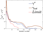
(a) LP: Convergence rate.

(b) LP: Limit search.

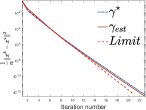
(c) QP: Convergence rate.

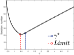
(d) QP: Limit search.

Figure 1: Linear and Quadratic Programming (zero initialization)

6.1.2 Structure-based initialization

Here, we would test the structure-based initialization discussed in Section 4.6.2. For LP, the initialization is set to $\bm{\zeta}^{0}=\bm{A}^{T}(\bm{AA}^{T})^{-1}\bm{b}$. For QP, the initialization is set to $\bm{\zeta}^{0}=(\bm{a}+\bm{b})/2$. The optimal step-size choice $\gamma^{\star}$ is obtained by solving the degree-4 polynomial, with closed-form expression in (4.30).

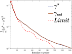
(a) LP: Convergence rate.

(b) LP: Limit search.

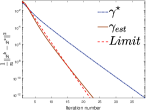
(c) QP: Convergence rate.

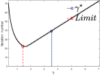
(d) QP: Limit search.

Figure 2: Linear and Quadratic Programming (structure-based initialization)

Remarks 6.1 (performance comparison).

For LP, the structure-based initialization outperforms the zero initialization setting. Recall that the ADMM fixed-point for LP is any point from $\{\beta\bm{x}^{\star}+\bm{\lambda}^{\star}/\beta\}_{\beta\in\mathbb{R}_{++}}$. Here, we initialize the primal part $\bm{x}^{\star}$ via a pseudo-inverse, which is relatively good. Meanwhile, we set the dual part $\bm{\lambda}^{\star}$ as a zero vector, which is also relatively good. The good performance is hence not surprising. On the other hand, for QP, the mean initialization $(\bm{a}+\bm{b})/2$ is relatively good for $\bm{x}^{\star}$, but setting $\bm{\lambda}^{\star}$ as a zero vector is a bad estimation. Its performance is therefore worse than zero initialization.

6.2 LAD and Huber fitting

Following the standard setup from [1], we test the following LAD problem :

$$\text{minimize}\,\,\|\bm{Ax}-\bm{b}\|_{1}$$ (6.3)

with variable $\bm{x},\bm{b}\in\mathbb{R}^{100},\bm{A}\in\mathbb{R}^{1000\times 100}$. The elements of $\bm{A}$ and $\bm{x}$ are generated from a normal distribution $\mathcal{N}(0,1)$ and $\mathcal{N}(0,10)$, respectively. $\bm{b}$ is set to equal to $\bm{A}\bm{x}$, and a randomly selected 20 elements of it are added with a random Gaussian noise $\mathcal{N}(0,100)$.

Following the standard setup from [1], we test the following Huber fitting problem:

$$\text{minimize}\,\,g(\bm{Ax}-\bm{b})$$ (6.4)

with variable $\bm{x}\in\mathbb{R}^{200},\bm{b}\in\mathbb{R}^{5000},\bm{A}\in\mathbb{R}^{5000\times 200}$, where function $g$ is defined in (5.4). The elements of $\bm{A},\bm{x}$ are generated from a normal distribution $\mathcal{N}(0,1)$. The columns of $\bm{A}$ are normalized. $\bm{b}$ is set to equal to $\bm{A}\bm{x}+\bm{\epsilon}_{1}+\bm{\epsilon}_{2}$, where $\bm{\epsilon}_{1}$ is an additive Gaussian noise from $\mathcal{N}(0,0.1)$; $\bm{\epsilon}_{2}$ is a sparse uniformly distributed noise from $[0,1]$ with density $0.04$.

As aforementioned in Section 4.6.2, for $l_{1}$ norm regularized problems, zero initialization should be generally good. We therefore limit our discussion to zero initialization here. The step-size choice is specified in (5.5).

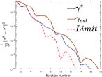
(a) LAD: Convergence rate.

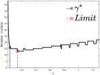
(b) LAD: Limit search.

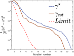
(c) HF: Convergence rate.

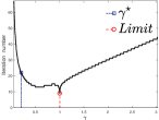
(d) HF: Limit search.

Figure 3: LAD and Huber fitting (zero initialization)

Remarks 6.2 (performance).

From Figure 3, we observe that the optimal step-size choice is close to the Limit. The estimated step-size choice has similar performance compared to the theoretical result.

6.3 Basis Pursuit and Lasso

Following the standard setup from [1], we test the following BP problem:

$$\text{minimize}\,\,\|\bm{x}\|_{1}\quad\text{subject to}\,\,\bm{Ax}=\bm{b},$$ (6.5)

with variable $\bm{x}\in\mathbb{R}^{30},\bm{b}\in\mathbb{R}^{10},\bm{A}\in\mathbb{R}^{10\times 30}$. The elements of $\bm{A},\bm{x}$ are generated from a normal distribution $\mathcal{N}(0,1)$. $\bm{x}$ is assumed sparse, with density factor $0.1$. $\bm{b}$ is set to equal to $\bm{A}\bm{x}$.

Following the standard setup from [1], we test the following Lasso problem:

$$\text{minimize}\,\,\|\bm{Ax}-\bm{b}\|^{2}+\alpha\|\bm{x}\|_{1}$$ (6.6)

with variable $\bm{x}\in\mathbb{R}^{5000},\bm{b}\in\mathbb{R}^{1500},\bm{A}\in\mathbb{R}^{1500\times 5000}$. The elements of $\bm{A},\bm{x}$ are generated from a normal distribution $\mathcal{N}(0,1)$. $\bm{x}$ is assumed sparse, with density factor $0.02$. The columns of $\bm{A}$ are normalized. $\bm{b}$ is set to equal to $\bm{A}\bm{x}+\bm{\epsilon}$, where $\bm{\epsilon}$ is an additive Gaussian noise from $\mathcal{N}(0,\sqrt{0.001})$. Regularization parameter $\alpha$ is set to $0.1\|\bm{A}^{T}\bm{b}\|_{\infty}$.

As aforementioned in Section 4.6.2, for $l_{1}$ norm regularized problems, zero initialization should be generally good. We therefore limit our discussion to zero initialization here. The step-size choice is specified in (5.7).

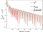
(a) BP: Convergence rate.

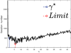
(b) BP: Limit search.

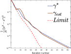
(c) Lasso:Convergence rate.

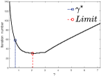
(d) Lasso: Limit search.

Figure 4: Basis Pursuit and Lasso (zero initialization)

Remarks 6.3 (performance).

From Figure 4, we observe that the optimal step-size choice is relatively close to the Limit. The estimated step-size choice has similar performance as the theoretical result.

6.4 TV and SICS

Following the standard setup from [1], we test the following TV problem:

$$\text{minimize}\,\,\text{minimize}\,\,\frac{1}{2}\|\bm{x-b}\|^{2}+\alpha\sum_{i}|x_{i+1}-x_{i}|$$ (6.7)

with variable $\bm{x},\bm{b}\in\mathbb{R}^{100},\bm{A}\in\mathbb{R}^{10\times 30}$. $\bm{x}$ is first set to be a ones vector and then randomly scaled on randomly selected entries. $\bm{b}$ is set to equal to $\bm{x}+\bm{\epsilon}$, where $\bm{\epsilon}$ is an additive Gaussian noise from $\mathcal{N}(0,1)$. Regularization parameter $\alpha$ is set to 5.

Following the standard setup from [1], we test the following SICS problem:

$$\text{minimize}\,\,\text{trace}(\bm{SX})-\text{logdet}(\bm{X})+\|\bm{X}\|_{1}$$ (6.8)

with variable $\bm{X,S}\in\mathbb{S}^{100}$. $\bm{S}$ is the covariance matrix of a random Gaussian matrix $\bm{D}\in\mathbb{R}^{1000\times 100}$ of mean 0.

As aforementioned in Section 4.6.2, for $l_{1}$ norm regularized problems, zero initialization should be generally good. We therefore limit our discussion to zero initialization here. The step-size choices are specified in (5.9) and (5.11).

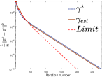
(a) TV: Convergence rate.

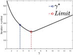
(b) TV: Limit search.

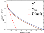
(c) SICS: Convergence rate.

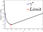
(d) SICS: Limit search.

Figure 5: TV and SICS (zero initialization)

Remarks 6.4 (performance).

From Figure 5, we observe that the optimal step-size choice is relatively close to the Limit. The estimated step-size choice has almost identical performance as the theoretical result.

6.5 SLR and Support vector machine

Following the standard setup from [1], we test the following SLR problem:

$$\text{minimize}\,\,\frac{1}{m}\sum_{i=1}^{m}log(1+exp(-{b_{i}}\langle\bm{a_{i}},\bm{w}\rangle+{v}))+\mu\|\bm{w}\|_{1}$$ (6.9)

with variable $\bm{x}\overset{\mathclap{\text{def}}}{=}[v,\bm{w}]^{T}\in\mathbb{R}^{51}$, $v\in\mathbb{R},\bm{w}\in\mathbb{R}^{50}$, $m=200$, $\mu=0.0094$. The elements of $v,\bm{w}$ are randomly generated from normal distribution $\mathcal{N}(0,1)$. $\bm{w}$ is set to be sparse with density factor $0.1$. $\bm{b}\in\mathbb{R}^{m}$ denotes a vector of labels corrupted by additive Gaussian noise from $\mathcal{N}(0,\sqrt{0.1})$. We refer the interested readers to [1] for the detailed process of generating such labels.

Following the standard setup from [1], we test the following Support vector machine (SVM) problem:

$$\underset{\bm{w},b}{\text{minimize}}\,\,\frac{1}{2}\|\bm{w}\|_{2}^{2}+\sum_{i=1}^{N}(\bm{A}_{i}[\bm{w}_{i},b_{i}]^{T}+\bm{1})_{+}$$ (6.10)

where $N=100$. We refer the interested readers to [1] and their open-sourced code for the detailed process of generating the positive and negative examples, and a worst-case partitioning. The complicated details is omitted here as our setting is kept exactly the same as theirs.

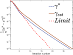
(a) SLR: Convergence rate.

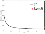
(b) SLR: Limit search.

(c) SVM: Convergence rate.

(d) SVM: Limit search.

Figure 6: SLR and SVM (zero initialization)

Remarks 6.5 (performance).

From Figure 6, we observe that the optimal step-size choice is close to the Limit. The estimated step-size choice has a similar performance as the theoretical result.

Remarks 6.6 (SLR infeasible step-size).

For the SLR problem, the open-source code from [1] employs a Newton-type gradient method to solve the x-update sub-problem in ADMM. The step-size is therefore no longer arbitrary. From Figure 6(b), we see that the largest feasible step-size is exactly the best choice, and any choice larger than it will cause the algorithm not converging.

7 Conclusion

In this work, we propose a general optimal step-size choice for ADMM given any initialization. The technique is based on optimizing a convergence rate bound, and only basic assumptions are imposed. Quite remarkably, the choice always admits a unique closed-form expression, and therefore easy to use. Numerical results show that such a choice is close to the underlying best choice (found by exhaustive search). Our technique also reveals the optimal initialization choices. Particularly, if one chooses initialization and step-size jointly optimal, then ADMM converges in exactly one iteration.

References

- [1] Stephen Boyd, Neal Parikh, Eric Chu, Borja Peleato, Jonathan Eckstein, et al. Distributed optimization and statistical learning via the alternating direction method of multipliers. Foundations and Trends® in Machine learning, 3(1):1–122, 2011.
- [2] Roland Glowinski and Americo Marroco. Sur l’approximation, par éléments finis d’ordre un, et la résolution, par pénalisation-dualité d’une classe de problèmes de dirichlet non linéaires. Revue française d’automatique, informatique, recherche opérationnelle. Analyse numérique, 9(R2):41–76, 1975.
- [3] Daniel Gabay and Bertrand Mercier. A dual algorithm for the solution of nonlinear variational problems via finite element approximation. Computers & mathematics with applications, 2(1):17–40, 1976.
- [4] Bartolomeo Stellato, Goran Banjac, Paul Goulart, Alberto Bemporad, and Stephen Boyd. Osqp: An operator splitting solver for quadratic programs. Mathematical Programming Computation, 12(4):637–672, 2020.
- [5] Goran Banjac and Paul J Goulart. Tight global linear convergence rate bounds for operator splitting methods. IEEE Transactions on Automatic Control, 63(12):4126–4139, 2018.
- [6] Pontus Giselsson and Stephen Boyd. Linear convergence and metric selection for douglas-rachford splitting and admm. IEEE Transactions on Automatic Control, 62(2):532–544, 2016.
- [7] Yuxiao Chen, Mario Santillo, Mrdjan Jankovic, and Aaron D Ames. Online decentralized decision making with inequality constraints: an admm approach. IEEE Control Systems Letters, 5(6):2156–2161, 2020.
- [8] Jianbo Ye and Jia Li. Scaling up discrete distribution clustering using admm. In 2014 IEEE International Conference on Image Processing (ICIP), pages 5267–5271. IEEE, 2014.
- [9] Terrence WK Mak, Minas Chatzos, Mathieu Tanneau, and Pascal Van Hentenryck. Learning regionally decentralized ac optimal power flows with admm. IEEE Transactions on Smart Grid, 2023.
- [10] Elsa Rizk, Stefan Vlaski, and Ali H. Sayed. Federated learning under importance sampling. IEEE Transactions on Signal Processing, 70:5381–5396, 2022.
- [11] Kun Yuan, Bicheng Ying, Stefan Vlaski, and Ali H. Sayed. Stochastic gradient descent with finite samples sizes. In 2016 IEEE 26th International Workshop on Machine Learning for Signal Processing (MLSP), pages 1–6, 2016.
- [12] Emmanuel J Candès and Terence Tao. The power of convex relaxation: Near-optimal matrix completion. IEEE Transactions on Information Theory, 56(5):2053–2080, 2010.
- [13] Jim Douglas and Henry H Rachford. On the numerical solution of heat conduction problems in two and three space variables. Transactions of the American mathematical Society, 82(2):421–439, 1956.
- [14] Jonathan Eckstein and Dimitri P Bertsekas. On the Douglas—Rachford splitting method and the proximal point algorithm for maximal monotone operators. Mathematical Programming, 55(1):293–318, 1992.
- [15] Michel Fortin and Roland Glowinski. Augmented Lagrangian methods: applications to the numerical solution of boundary-value problems. Elsevier, 2000.
- [16] Daniel O’Connor and Lieven Vandenberghe. On the equivalence of the primal-dual hybrid gradient method and Douglas–Rachford splitting. Mathematical Programming, 179(1):85–108, 2020.
- [17] Antonin Chambolle and Thomas Pock. A first-order primal-dual algorithm for convex problems with applications to imaging. Journal of mathematical imaging and vision, 40(1):120–145, 2011.
- [18] Ernie Esser, Xiaoqun Zhang, and Tony F Chan. A general framework for a class of first order primal-dual algorithms for convex optimization in imaging science. SIAM Journal on Imaging Sciences, 3(4):1015–1046, 2010.
- [19] Thomas Pock, Daniel Cremers, Horst Bischof, and Antonin Chambolle. An algorithm for minimizing the Mumford-Shah functional. In 2009 IEEE 12th International Conference on Computer Vision, pages 1133–1140. IEEE, 2009.
- [20] Neal Parikh and Stephen Boyd. Proximal algorithms. Foundations and Trends in optimization, 1(3):127–239, 2014.
- [21] Wei Shi, Qing Ling, Kun Yuan, Gang Wu, and Wotao Yin. On the linear convergence of the admm in decentralized consensus optimization. IEEE Transactions on Signal Processing, 62(7):1750–1761, 2014.
- [22] Euhanna Ghadimi, André Teixeira, Iman Shames, and Mikael Johansson. Optimal parameter selection for the alternating direction method of multipliers (ADMM): quadratic problems. IEEE Transactions on Automatic Control, 60(3):644–658, 2014.
- [23] Ernest K Ryu and Wotao Yin. Large-scale convex optimization: algorithms & analyses via monotone operators. Cambridge University Press, 2022.
- [24] Clarice Poon and Jingwei Liang. Trajectory of alternating direction method of multipliers and adaptive acceleration. Advances in Neural Information Processing Systems, 32, 2019.
- [25] Jingwei Liang, Jalal Fadili, and Gabriel Peyré. Local convergence properties of douglas–rachford and alternating direction method of multipliers. Journal of Optimization Theory and Applications, 172:874–913, 2017.
- [26] Jingwei Liang, Jalal Fadili, and Gabriel Peyré. Activity identification and local linear convergence of forward–backward-type methods. SIAM Journal on Optimization, 27(1):408–437, 2017.
- [27] Heinz H Bauschke and Patrick L Combettes. Convex Analysis and Monotone Operator Theory in Hilbert Spaces. Springer, 2017.
- [28] Patrick L Combettes and Noli N Reyes. Moreau’s decomposition in banach spaces. Mathematical Programming, 139(1):103–114, 2013.
- [29] Stephen P Boyd and Lieven Vandenberghe. Convex optimization. Cambridge university press, 2004.
- [30] Isaac (https://math.stackexchange.com/users/72/isaac). Is there a general formula for solving quartic (degree ) equations? Mathematics Stack Exchange. URL:https://math.stackexchange.com/q/786 (version: 2021-12-04).