Pre-training on Synthetic Driving Data for Trajectory Prediction

Abstract

Accumulating substantial volumes of real-world driving data proves pivotal in the realm of trajectory forecasting for autonomous driving. Given the heavy reliance of current trajectory forecasting models on data-driven methodologies, we aim to tackle the challenge of learning general trajectory forecasting representations under limited data availability. We propose to augment both HD maps and trajectories and apply pre-training strategies on top of them. Specifically, we take advantage of graph representations of HD-map and apply vector transformations to reshape the maps, to easily enrich the limited number of scenes. Additionally, we employ a rule-based model to generate trajectories based on augmented scenes; thus enlarging the trajectories beyond the collected real ones. To foster the learning of general representations within this augmented dataset, we comprehensively explore the different pre-training strategies, including extending the concept of a Masked AutoEncoder (MAE) for trajectory forecasting. Extensive experiments demonstrate the effectiveness of our data expansion and pre-training strategies, which outperform the baseline prediction model by large margins, e.g. 5.04%, 3.84% and 8.30% in terms of $MR_{6}$, $minADE_{6}$ and $minFDE_{6}$.

I Introduction

Trajectory forecasting is an important task for safely navigating autonomous vehicles in crowded traffic scenarios. The state-of-the-art trajectory forecasting models are empowered by data-driven supervised learning approaches, whose performance heavily relies on the scale of motion data available for training [1, 2, 3]. However, driving data is expensive and time-consuming to collect and annotate, which hinders cost-efficient scaling of training data as in Natural Language Processing (NLP) and Computer Vision (CV). Data-collection vehicles with sophisticated sensors need to run on public roads to collect traffic data. For instance, the Argoverse V1.1 dataset [4] and the Waymo Motion Dataset [1] consist of 324K and 103K driving scenes, which add up to a total of 320 and 574 hours of driving data, respectively. Notably, a substantially larger amount of raw data needs to be collected in order to filter out the given amount of high-quality training data. In addition to data collection, a significant amount of human labor is required to annotate the raw data into a cohesive dataset—traffic participants need to be annotated; and HD maps need to be aligned and integrated with the traffic data.

TABLE I: Effortless Driving Data Generation.

Dataset	Driving Hours	Scenes
Argoverse v1.1	320	324k
Synthetic Dataset	+0	+370k

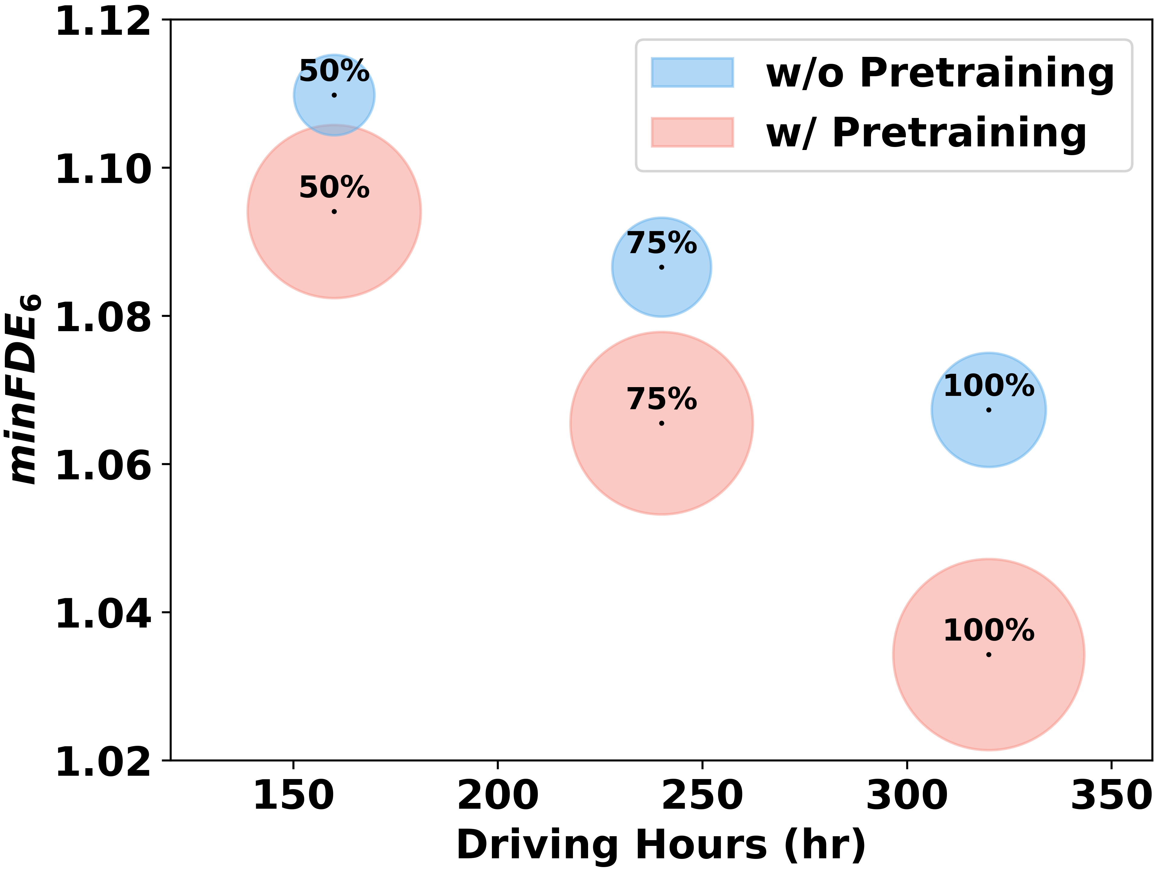
Figure 1: Our data synthesis and self-supervised pre-training pipeline enhances prediction performance without extra real-world driving data. The area of each circle is proportional to the number of driving scenes used, including the synthetic and real ones. The numbers in the circles indicate the percentages of real-world driving data from the Argoverse dataset used for fine-tuning. (A lower $minFDE_{6}$ is preferable.)

In this work, we sought to synthetic data as a solution to break through the data bottleneck in trajectory forecasting. We propose to automatically generate synthetic driving data to complement real-world data, enhancing the overall data diversity and utility. Compared to collecting and processing real-world data, which involve huge labor, generating synthetic data is effortless—as shown in Tab. I, our proposed data generation method only takes 20 computational hours to generate a comparable number of scenes to the real-world dataset. Yet, as shown in Fig. 1, the synthetic data can improve the prediction accuracy and data efficiency when paired with our proposed training pipeline.

Concretely, our proposed data generation consists of two parts: 1) map augmentation; and 2) trajectory generation. For map augmentation, we adopt the vector-transformation method proposed in [5] to convert the linear lanes found in real-world maps into curved lanes within a defined range of sharpness and angle, as shown in Fig. 2 (upper-left). The augmented curved roads are introduced to diversify the map data—curved lanes occur at significantly low frequency in real-world data. Subsequently, we navigate a simulated vehicle on both real-world and augmented maps with a rule-based planner [6] to generate trajectory data. The rule-based planner leverages prior knowledge to facilitate the realism of the generated trajectories.

Despite our efforts to improve the realism of the generated data, there still exists considerable discrepancy between the synthetic and real-world data. One crucial question is how to efficiently utilize the synthetic data to foster prediction performance while minimizing the impact of the domain gap. To answer this question, we conducted an extensive study on different training algorithms to use the synthetic data. In particular, we compare three different paradigms: augmenting the real-world prediction dataset [7, 8, 9], supervised pre-training [10, 11, 12], and self-supervised pre-training [13, 14, 15, 16, 17, 18, 19, 20, 21, 22]. As for directly augmenting the prediction dataset, we disregard the domain gap and mix the synthetic and real data to train the prediction model directly. In our supervised pre-training paradigm, we first pre-train the model for the supervised trajectory prediction task on the synthetic dataset, and then fine-tune the model on the real dataset. While the pre-training and fine-tuning tasks are both supervised prediction tasks, the two-stage scheme is introduced to mitigate the bias due to the domain gap. Further, in self-supervised pre-training, we substitute the supervised pre-training task with self-supervised masked reconstruction tasks [17] tailored to trajectory forecasting, i.e., map reconstruction, trajectory reconstruction, or a combination of both. The goal is to train a generalizable scene representation on the synthetic data that oversees detailed domain-specific information and can benefit cross-domain fine-tuning. Extensive experiments conducted on the Argoverse dataset with denseTNT backbone demonstrate that self-supervised pre-training outperforms the other two ways. With our synthetic data generation and self-supervised pre-training pipeline, the fine-tuned model outperforms the baseline model by a large margin—5.04%, 3.84%, and 8.30% in terms of $MR_{6}$, $minADE_{6}$ and $minFDE_{6}$. Detailed ablation studies are then conducted to shed light on the influence of some subtle factors on prediction performance, such as information leak and map augmentation.

Our contributions are summarized as follows:

• We propose to leverage synthetic map and trajectory data to address the data scarcity issue in trajectory forecasting with minimal cost. In particular, we introduce a novel data generation scheme that consists of geometric-based map augmentation and rule-based trajectory generation.

• We conducted extensive experiments to pinpoint the best training scheme to utilize the synthetic data. Our results show that self-supervised pre-training is the most effective one among the three tested paradigms: augmenting the training dataset, supervised pre-training, and self-supervised pre-training.

• With our synthetic data generation and self-supervised pre-training pipeline, the fine-tuned model outperforms the baseline model by a large margin—5.04%, 3.84%, and 8.30% in terms of $MR_{6}$, $minADE_{6}$ and $minFDE_{6}$.

II Related Works

II-A Data Augmentation in Trajectory Prediction

Data scarcity is a bottleneck for exploring the model’s capacity for better performance [3]. To address this issue, numerous data augmentation techniques, such as the application of image transformations [15, 23, 24] and utilization of synthetic data [25, 26, 27, 24], are introduced in the CV community to augment or replicate seldom-seen real-world scenes. While these methods expand the dataset, they also introduce a domain gap between the real-world distribution and their augmented counterparts. In the trajectory prediction problem, the unique properties of trajectory and map data necessitate a specific design for data augmentation or generation that is both reasonable and cost-effective. In [28]’s approach, a simple augmentation technique is applied to the vehicle’s velocity properties to mimic unpredictable driver behaviors in anticipation of future trajectories based on past history. Additionally, [5] proposes the use of map augmentation techniques to alter the topological semantics of map information as adversarial attacks on current trajectory prediction models. While these methods expand the dataset size, their additional trajectories are simple geometric transformations of existing lane elements or trajectories, without careful consideration of the feasibility and realism of the transformed trajectories. In our work, we enhance the map data to supplement limited features, like curves and turns, and employ a rule-based simulation to mimic reasonable traffic behaviors for trajectory generation.

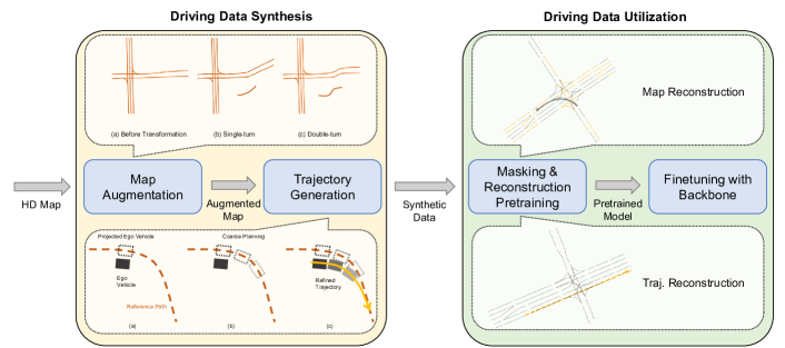
Figure 2: Pipeline of driving data synthesis and utilization. We augment the map and generate trajectory on it to acquire synthetic motion data, which are then used for pre-training via masking and reconstruction. The pre-trained model is used to initialize the backbone model during fine-tuning.

II-B Pre-training in Trajectory Prediction

Pre-training is effective for the data shortage problem in trajectory prediction. In [3], contrastive learning was used to cluster similar map patches and establish associations between map patches and the trajectory, thereby fully utilizing the existing map data. In [29], four pre-training tasks were initiated, including randomly masking and recovering parts of the features, to enhance the encoding. Concurrently to our work, [30, 31] used MAE to pre-train the encoder. However, these methods did not introduce any new data. Another work [28] generated a pseudo trajectory that strictly follows the lanes for pre-training. However, this strict compliance hinders the realism of the pseudo trajectories. In contrast, our work aims to generate realistic synthetic trajectories to mitigate the domain gap between the synthetic and real data.

While limited efforts on pre-training exist in the trajectory forecasting literature, some auxiliary tasks have been introduced to regularize trajectory prediction models during training. [32] introduced a feature-masking task to encourage feature interactions, which inspired us to use methods in CV [17] and NLP [18] to stimulate feature interactions in the learned scene representation. Taking cues from these works, we investigated masked reconstruction as a self-supervised pre-training method to utilize the synthetic data.

III Methods

III-A Synthetic Map and Trajectory Data Generation

III-A1 Map Data Augmentation

Considering the lack of curve trajectory in the real-world training dataset, we add the map augmentation module to our data synthesis pipeline. Inspired by the conditional adversarial scene generation process proposed in [5], we design transformation functions that alter the original map topology, as shown in Fig. 2 (upper-left). Given that each scene is composed of a set of scene points, we define the transformation on each scene point $(s_{x},s_{y})$ in the following form:

$$\overline{s}=(s_{x},s_{y}+f(s_{x}-b))$$ (1)

where $\overline{s}$ is the transformed point, $f$ is the single-variable transformation function, and $b$ is a parameter that determines the region of applying the transformation, i.e., we only modify the scene points whose x-coordinates surpass $b$. We further adopt the following two transformation functions for our map augmentation process.

Single-turn introduces a single turning on the roadway. The transformation function for single-turn is defined as:

$$f_{\mathrm{single-turn}}(s_{x})=\begin{cases}0,&s_{x}<0,\\ q_{\alpha}(s_{x}),&0\leq s_{x}\leq s_{t}\\ (s_{x}-s_{t})q_{\alpha}^{\prime}(s_{t})+q_{\alpha}(s_{t}),&s_{t}<s_{x}\\ \end{cases}$$ (2)

where $s_{t}$ represents the length of the turn and $q_{\alpha}$ is an auxiliary function defined by

$$q_{\alpha}(s_{x})=\frac{\alpha_{1}}{s_{t}^{\alpha_{2}}}s_{x}^{\alpha_{2}}$$ (3)

where $\alpha_{1},\alpha_{2}$ are the parameters to control the turn’s sharpness and angle. Note the $q_{\alpha}^{\prime}$ is simply the derivative of $q_{\alpha}$. Our formulation of $f_{\mathrm{single-turn}}(s_{x})$ is continuously differentiable and thus makes a smooth augmented single-turn curve.

Double-turn introduces two consecutive smooth single-turns in opposite directions to the road. The transformation function for double-turn is based on the that of single-turn:

$$f_{\mathrm{double-turn}}(s_{x})=f_{\mathrm{single-turn}}(s_{x})-f_{\mathrm{single-turn}}(s_{x}-\beta)$$ (4)

where $\beta$ is the distance between two turns. In practice, we randomly select single-turn or double-turn augmented lanes and randomly assign values in a specific range to ensure a reasonable extent of transformation, as shown in Tab. II.

III-A2 Trajectory Data Generation

To generate labeled trajectory data on both real-world and augmented maps, we implement a trajectory data generator to synthesize pseudo-expert trajectories in single-car scenarios, as illustrated in Fig. 2 (bottom-left). Following the motion data generation pipeline proposed in [6], we began by projecting its position onto the nearest reference path obtained from the training dataset in order to determine the optimal trajectory for the ego vehicle. Subsequently, we utilize the A^∗ planning method on this reference path to generate a preliminary, coarse trajectory. Specifically, we define a node $n_{i}$ in the search space by a tuple $(s_{i},v_{i},t_{i})$, which respectively represents the ego vehicle’s coordinate, velocity, and time on the reference path. A transition from $n_{i}$ to $n_{i+1}$ defines the $n_{i+1}$ by:

$$(s_{i+1},v_{i+1},t_{i+1})=(s_{i}+v_{i}\delta t+\frac{1}{2}a\delta t^{2},v_{i}+a\delta t,t_{i}+\delta t)$$ (5)

where $a$ denotes the acceleration and $\delta t$ denotes the minimum time interval for coarse planning. The cost function of the transition is given as:

$$\mathcal{C}(n_{i},a,n_{i+1})=w_{1}a^{2}+w_{2}\kappa(s_{i+1})v_{i+1}^{2}+w_{3}(v_{i+1}-v_{d})^{2}$$ (6)

where $w_{1},w_{2},w_{3}$ are weights for each term, $\kappa(s_{i+1})$ denotes curvature of reference path at $s_{i+1}$, and $v_{d}$ denotes desired driving velocity set in prior. The planning process concludes when the time associated with the searched node surpasses the end time $t_{g}$, resulting in the conversion of the resultant path into a coarse trajectory $s_{c}(t)$ within the global frame. The hyperparameters adopted for the synthetic trajectory generation pipeline are listed in Tab. II. Finally, we introduce an additional refinement procedure to map the initial state of the final pseudo-expert trajectory to the current state of the ego car. Concretely, we solve the following optimization problem to acquire the refined trajectory $s_{r}(t)$:

$$\footnotesize\min_{s_{r}} \sum^{t_{g}}_{T=\delta\hat{t}}\omega_{1}a_{r}(T)^{2}+\omega_{2}j_{r}(T)^{2}+\sum^{t_{g}}_{T=k\delta\hat{t}}\omega_{3}(s_{r}(T)-s_{c}(T))^{2}$$

s.t. $$\quad v_{r}(T_{0})=v_{0}\quad\text{and}\quad s_{r}(T_{0})=s_{0}$$ (7)

where $\omega_{1},\omega_{2},\omega_{3}$ are weights for each term, $a_{r},j_{r}$ are refined acceleration and jerk, $\delta\hat{t}$ is the fine-grained time step such that $k\delta\hat{t}=\delta t$. $v_{0},s_{0}$ corresponds to the ego car’s initial velocity and position.

TABLE II: Parameter selection for data synthesis.

Traj. Param.	Value	Map Param.	Value
$a$	$\in[-2,1]$	$s_{x}$	10
$w_{1}$	5	$\alpha_{1}$	$\in[1,10]$
$w_{2}$	5	$\alpha_{2}$	20
$w_{3}$	1	$s_{t}$	10
$v_{d}$	$\in[6,15]$	$\beta$	20

III-B Utilization of Synthetic Data

To make maximum use of synthetic data while avoiding the influence of domain gaps, we comprehensively study several candidate approaches to identify the best strategy. The first approach is to directly combine the synthetic and real data for training, i.e. treating them identically. While this method is fairly straightforward, it also introduces bias into the model due to the domain gap between the synthetic and real data. Another method is supervised pre-training: we first pre-train the model for the supervised trajectory prediction task on the synthetic dataset, and then fine-tune the model on the real dataset. While the pre-training and fine-tuning tasks are both supervised prediction tasks, the two-stage scheme is introduced to mitigate the bias caused by the domain gap. To further mitigate the influence of the domain gap, finally, we investigate the self-supervised pre-training method which is elaborated in the following subsection.

III-C Self-supervised Pre-training Framework

We adapt MAE [17] into a self-supervised pre-training framework for trajectory forecasting. The goal is to learn a generalizable scene representation that can well capture the interactions between lanes and the ones between lanes and trajectories from the synthetic data. During the pre-training stage, a specific percentage of trajectories or map lanes are masked, challenging the model to reconstruct the masked segments. The masked objects are replaced with mask tokens, which are learned and shared parameters that signal the existence of a masked object to be reconstructed [17]. Positional encoding is added to provide the subordinate and sequential information. Though specific information is removed in mask tokens, they still provide the model with where the masked information is. Such information leak will lead the model to find a shortcut to interpolate missing information instead of to reconstruct them by context understanding [33]. To prevent this, only the unmasked elements are processed through the backbone’s encoder. Thereafter, the masked tokens, in combination with the encoded unmasked parts, are fed into a shallow transformer decoder to reconstruct the masked parts. Upon completion of the pre-training phase, the backbone model is initialized using the encoder parameters of the pre-trained model, and then fine-tuned on real-world data for the prediction task. This approach enables the model to acquire general semantics during the pre-training stage while discarding extraneous details.

III-D Masking Strategy

We propose and compare different design options for masking and reconstruction during the pre-training stage:

III-D1 Map Reconstruction

Map reconstruction is proposed to foster the encoder to capture the lane features and their interactions. The masking policies and reconstruction procedures are illustrated in Fig. 2 (upper-right). We randomly choose 50% lanes as masking lanes, replacing everything but the coordinate information for their first points with mask tokens. These masked objects, together with the encoded features of the unmasked objects, are then fed into the decoder. Utilizing lane-wise interactions, the feature of the masked lanes would be recovered. Point-wise L1 loss is employed across all our experiments. The loss function of map reconstruction $l_{map}$ is defined as the difference between the reconstructed lane and the ground-truth one.

III-D2 Trajectory Reconstruction

Trajectory reconstruction is introduced to improve the model’s understanding of the trajectory features and the interactions between the trajectory and map elements, as shown in Fig. 2 (bottom-right). Since the synthetic scene only consists of one agent, only a single trajectory is masked in each scene. We retain its starting point in the masked object as in map reconstruction. To prevent modal collapse, the decoder is allowed to produce six potential trajectories. We select the one with the minimum loss to define the loss function $l_{traj}$. Additionally, to ensure that all modes are activated, we add the weighted reconstruction errors of the remaining modes to the loss function as regularization. A weight of 0.05 is used in our experiments.

III-D3 Combination of Map and Trajectory Reconstructions

We integrate both map and trajectory reconstruction tasks by randomly selecting a percentage of scenes within a mini-batch to conduct either of the reconstructions. This selection is achieved by generating a random number prior to masking each scene. As a result, the same scene could undergo different reconstruction tasks across various epochs. The overall loss function is computed as the average of the individual scene-specific losses previously described.

IV Experiments

IV-A Experiment Setup

Synthetic Dataset. The pre-training dataset is generated in accordance with the methods outlined in Sec. III-A. The Map is sourced from the HD maps and APIs in the Argoverse v1.1 Motion Forecasting Dataset [4]. We generate trajectories on both the original map and the augmented map. The resultant generated dataset contains 370k scenes, where 205k are generated on the original map and 165k are generated on the augmented map. Each generated scene contains the vehicle’s position spanning 5 seconds, following the format of the Argoverse v1.1 Motion Forecasting Dataset. As visualized in Fig. 4, the generated data align well with a vast spectrum of velocities present in the real-world data distribution.

Argoverse v1.1 Motion Forecasting Dataset. The Argoverse v1.1 Motion Forecasting Dataset [4] is a renowned dataset frequently employed in vehicle motion prediction studies. It consists of 324k scenes, each spanning 5 seconds and sampled at 10 Hz. In every scene, the initial 2 seconds serve as the history, while the subsequent 3 seconds are designated for prediction. Additionally, the dataset also includes HD maps collected from Pittsburgh and Miami, covering all the scenes in the dataset. There are 205k and 39k scenes in the training and validation sets, respectively, in which the validation set is used for evaluating our model.

Evaluation Metrics. Following Argoverse’s benchmark, we use miss rate ($MR_{6}$), minimum final displacement error ($minFDE_{6}$), and minimum average displacement error ($minADE_{6}$) as the evaluation metrics. The subscripts mean that the minima are computed over six predicted trajectories.

Implementation Details. In our experiments, we adopt DenseTNT [34] as the prediction backbone. DenseTNT uses Vectornet [32] as its encoder which adopts a vectorized scene representation, i.e., the lanes and trajectories are represented as vectors, which makes the masking process straightforward. The pre-training is conducted on a Nvidia A6000 GPU with a batch size of 256. The learning rate is $10^{-5}$ for trajectory reconstruction and $10^{-3}$ for map reconstruction. For mixed map and trajectory reconstructions, we use a learning rate of $10^{-4}$. Except for the GPU, all other fine-tuning settings are the same as in DenseTNT [34]. During evaluation, we choose the 100ms optimization for $minFDE_{6}$.

IV-B Comparison of Different Training Methods

TABLE III: Method Comparison for Using Synthetic Data.

Method	Pretrain Task	$MR_{6}$(%) ($\downarrow$)	$minFDE_{6}$ ($\downarrow$)	$minADE_{6}$ ($\downarrow$)
Baseline	/	9.73	1.0673	0.8052
Dataset Augmentation	/	9.45	1.0567	0.7432
Supervised whole PT	Prediction	9.34	1.0371	0.7551
Supervised encoder PT	Prediction	9.20	1.0369	0.7639
Self-supervised PT	Reconstruction	9.24	1.0263	0.7384

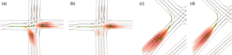
Figure 3: Performance comparison without or with pre-training. The green line and star indicate the true trajectory and its last point, while orange ones are the predicted ones. The orange background shows the possibility of each point being the predicted last point of the trajectory. (a) and (b) show the prediction results without or with trajectory pre-training. (c) and (d) illustrate the performance without or with map pre-training.

We compare the performances of multiple methods described in Sec. III-B. The results are shown in Tab. III. While directly augmenting the training dataset can slightly improve the prediction accuracy, it does not perform as well as pre-training approaches. The result is consistent with our motivation behind adopting pre-training methods. For supervised pre-training methods, we compared two alternative fine-tuning strategies: initializing the entire model with the pre-trained model or only initializing the encoder with the pre-trained one. We found that the decoder does not benefit from loading the parameters from the pre-trained model. Our hypothesis is that the domain-specific nuances learned by the decoder during supervised pre-training might not generalize well to real-world scenarios. It implies that the synthetic data is most suitable for improving representation learning rather than directly improving the entire backbone model for trajectory prediction. To this end, self-supervised pre-training should be the most efficient way to utilize the synthetic data, as the training tasks are deliberately designed for learning generalizable scene representation, which is supported by the experimental results—The self-supervised pre-trained model achieves the best prediction accuracy after fine-tuning.

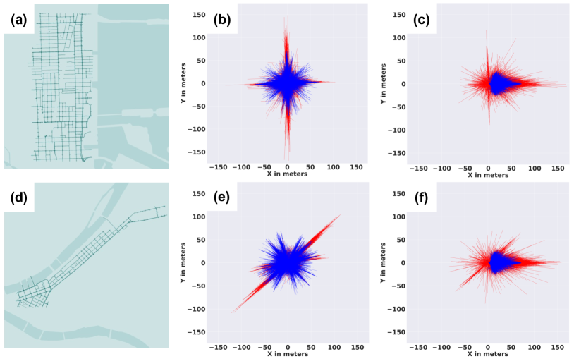
Figure 4: Data distribution comparison between synthetic dataset (blue) and the real-world dataset (red) in terms of the speed and direction properties. (a) represents the map representation for MIA city. (b) represents the trajectory distribution of scenes in (a), showing a pattern of divergence in velocity properties. (c) represents the trajectory distribution of scenes in (b) rotated to the same initial direction, demonstrating a pattern of divergence in direction properties. (d)(e)(f) are the counterparts of (a)(b)(c) in PIT city.

IV-C Comparison of Self-Supervised Pre-training Tasks

TABLE IV: Performance of Self-Supervised Pre-Training.

Method	$MR_{6}$(%) ($\downarrow$)	$minFDE_{6}$ ($\downarrow$)	$minADE_{6}$ ($\downarrow$)
Baseline	9.73	1.0673	0.8052
Map Reconstruction	9.20 (-5.45%)	1.0343 (-3.09%)	0.7571 (-5.97%)
Trajectory Reconstruction	9.24 (-5.04%)	1.0263 (-3.84%)	0.7384 (-8.30%)
Combined Reconstruction	9.27 (-4.73%)	1.0349 (-3.04%)	0.7284 (-9.54%)

We present the experimental results of different self-supervised pre-training tasks in Tab. IV. The results show that all of the self-supervised pre-training tasks can substantially improve the prediction accuracy compared with the baseline. Specifically, with map reconstruction, an $MR_{6}$ of 9.20% is observed, which is 5.04% lower than the baseline. Trajectory reconstruction pre-training helps improve the $minFDE_{6}$ by 3.84% compared to the baseline. Combining them together, when we allocate 70% scenes in a batch to map reconstruction and 30% scenes to trajectory reconstruction, we achieve a $minADE_{6}$ of 0.7284, marking an improvement of 9.54% against the baseline.

To elucidate the impact of our synthetic data and the pre-training, we provide qualitative examples in Fig. 3. Fig. 3 (a) and (b) contrast prediction outcomes without and with trajectory reconstruction pre-training. We observe that the model without pre-training predicts potential right-turn trajectories. However, since the target vehicle is not in the right-turn lane, its intention to go straight should be able to be identified, if the spatial relation between the historical trajectory and the lanes is captured by the encoder. In contrast, trajectory pre-training strengthens the model’s confidence in discerning the go-straight intention. Sub-figures (c) and (d) compare the prediction outcomes of the models without and with map reconstruction pre-training. In these sub-figures, the right-turn lane eventually merges with the 2^nd lane from the right. We observe that with map pre-training, the model is able to more accurately predict that the vehicle will not merge into the 1st lane from the right. This result aligns with expectations—map reconstruction enhances the model’s understanding of lane connectivity, thereby improving prediction accuracy.

V Discussion

In this section, we elaborate on some detailed design choices we made. In Sec. V-A, we validate the necessity of map augmentation. In Sec. V-B, we analyze the synthetic data distribution to further validate the necessity of self-supervised pre-training. In Sec. V-C, we look into the information leak problem and validate our pre-training model architecture choice, which avoids information leak and effectively improve fine-tuned performance.

V-A Benefits of Map Augmentation

TABLE V: Contributions of map augmentation.

Pretrain Dataset	$MR_{6}$(%)	$minFDE_{6}$	$minADE_{6}$
Baseline	9.73	1.0673	0.8052
Original Map	9.40	1.0517	0.7694
Original+Augmented Map	9.20	1.0343	0.7571

We assess the performance of models pre-trained with and without scenes generated on the augmented maps. As map augmentation influences the distribution of map elements more significantly, map reconstruction is selected as the pre-training task here for evaluation. The model trained on data with augmented maps significantly outperforms the other, as shown in Tab. V, underscoring the value of map augmentation in improving prediction models.

V-B Properties of Synthetic Data

Fig. 4 illustrates the disparity between the synthetic data and real-world data distributions concerning velocity and direction. While our synthetic dataset encompasses a broader spectrum of velocity than the real-world data, it is important to note the presence of outliers representing extreme velocity cases within the real-world data. Additionally, the real-world dataset encompasses a multitude of scenarios with pronounced turning angles, such as U-turns, which pose challenges in terms of accurate generation within the synthetic dataset. The discrepancy in data distributions validates that self-supervised pre-training is necessary to mitigate the impact of distributional shifts.

V-C Information Leak in Self-supervised Pre-training

TABLE VI: Influence of Information Leak.

Pretrain Method	$MR_{6}$(%)	$minFDE_{6}$	$minADE_{6}$
Baseline	9.73	1.0673	0.8052
No Info Leak Traj PT	9.24	1.0263	0.7384
W/ Info Leak Traj PT	9.45	1.0520	0.7581
No Info Leak Map PT	9.20	1.0343	0.7571
W/ Info Leak Map PT	9.84	1.0735	0.7614

In our work, we adopt a method similar to MAE [17], where the mask tokens are not passed to the encoder. While this eliminates the information leak from mask tokens, the encoder also loses the first point coordinates attached to masked objects. We, therefore, compare the prediction results both with or without information leak. In both scenarios, we ensure that the mask tokens pass through an equal number of transformer layers (i.e. one in our case) to exchange information. As shown in Tab. VI, we observe that the configuration without information leakage significantly outperforms its counterpart, affirming that the risk of information leakage outweighs the drawback of losing some positional data.

VI Conclusion

To expand and diversify the scant motion data for trajectory prediction, we efficiently generate vehicle trajectory using both the original map and its augmented variant in this study. We evaluate strategies for optimizing data utilization and find out that self-supervised pre-training is the most effective strategy. With our synthetic data generation and self-supervised pre-training pipeline, the fine-tuned prediction model outperforms the baseline by a large margin. Our research offers a comprehensive pipeline for data generation and utilization, providing a promising direction to alleviate the data scarcity problem in trajectory forecasting.

References

- [1] S. Ettinger, S. Cheng, B. Caine, C. Liu, H. Zhao, S. Pradhan, Y. Chai, B. Sapp, C. R. Qi, Y. Zhou, Z. Yang, A. Chouard, P. Sun, J. Ngiam, V. Vasudevan, A. McCauley, J. Shlens, and D. Anguelov, “Large scale interactive motion forecasting for autonomous driving: The waymo open motion dataset,” in Proceedings of the IEEE/CVF International Conference on Computer Vision (ICCV), October 2021, pp. 9710–9719.
- [2] F. Yu, H. Chen, X. Wang, W. Xian, Y. Chen, F. Liu, V. Madhavan, and T. Darrell, “Bdd100k: A diverse driving dataset for heterogeneous multitask learning,” in Proceedings of the IEEE/CVF conference on computer vision and pattern recognition, 2020, pp. 2636–2645.
- [3] C. Xu, T. Li, C. Tang, L. Sun, K. Keutzer, M. Tomizuka, A. Fathi, and W. Zhan, “Pretram: Self-supervised pre-training via connecting trajectory and map,” in Computer Vision – ECCV 2022, S. Avidan, G. Brostow, M. Cissé, G. M. Farinella, and T. Hassner, Eds. Cham: Springer Nature Switzerland, 2022, pp. 34–50.
- [4] M.-F. Chang, J. Lambert, P. Sangkloy, J. Singh, S. Bak, A. Hartnett, D. Wang, P. Carr, S. Lucey, D. Ramanan, et al., “Argoverse: 3d tracking and forecasting with rich maps,” in Proceedings of the IEEE/CVF Conference on Computer Vision and Pattern Recognition, 2019, pp. 8748–8757.
- [5] M. Bahari, S. Saadatnejad, A. Rahimi, M. Shaverdikondori, A.-H. Shahidzadeh, S.-M. Moosavi-Dezfooli, and A. Alahi, “Vehicle trajectory prediction works, but not everywhere,” in Proceedings of the IEEE/CVF Conference on Computer Vision and Pattern Recognition (CVPR), 2022.
- [6] Z.-H. Yin, C. Li, L. Sun, M. Tomizuka, and W. Zhan, “Iterative imitation policy improvement for interactive autonomous driving,” ArXiv, vol. abs/2109.01288, 2021.
- [7] Z. Zhong, L. Zheng, G. Kang, S. Li, and Y. Yang, “Random erasing data augmentation,” in Proceedings of the AAAI conference on artificial intelligence, vol. 34, no. 07, 2020, pp. 13 001–13 008.
- [8] K. Ryu, S. Hwang, and J. Park, “Instant domain augmentation for lidar semantic segmentation,” in Proceedings of the IEEE/CVF Conference on Computer Vision and Pattern Recognition (CVPR), June 2023, pp. 9350–9360.
- [9] S. Kim, S. Lee, D. Hwang, J. Lee, S. J. Hwang, and H. J. Kim, “Point cloud augmentation with weighted local transformations,” in Proceedings of the IEEE/CVF International Conference on Computer Vision (ICCV), October 2021, pp. 548–557.
- [10] K. He, R. Girshick, and P. Dollar, “Rethinking imagenet pre-training,” in Proceedings of the IEEE/CVF International Conference on Computer Vision (ICCV), October 2019.
- [11] D. Mahajan, R. Girshick, V. Ramanathan, K. He, M. Paluri, Y. Li, A. Bharambe, and L. van der Maaten, “Exploring the limits of weakly supervised pretraining,” in Proceedings of the European Conference on Computer Vision (ECCV), September 2018.
- [12] Y. Wei, Y. Zhang, J. Huang, and Q. Yang, “Transfer learning via learning to transfer,” in Proceedings of the 35th International Conference on Machine Learning, ser. Proceedings of Machine Learning Research, J. Dy and A. Krause, Eds., vol. 80. PMLR, 10–15 Jul 2018, pp. 5085–5094.
- [13] P. Vincent, H. Larochelle, I. Lajoie, Y. Bengio, P.-A. Manzagol, and L. Bottou, “Stacked denoising autoencoders: Learning useful representations in a deep network with a local denoising criterion.” Journal of machine learning research, vol. 11, no. 12, 2010.
- [14] M. Assran, Q. Duval, I. Misra, P. Bojanowski, P. Vincent, M. Rabbat, Y. LeCun, and N. Ballas, “Self-supervised learning from images with a joint-embedding predictive architecture,” in Proceedings of the IEEE/CVF Conference on Computer Vision and Pattern Recognition (CVPR), June 2023, pp. 15 619–15 629.
- [15] T. Chen, S. Kornblith, M. Norouzi, and G. Hinton, “A simple framework for contrastive learning of visual representations,” in International conference on machine learning. PMLR, 2020, pp. 1597–1607.
- [16] K. He, H. Fan, Y. Wu, S. Xie, and R. Girshick, “Momentum contrast for unsupervised visual representation learning,” in Proceedings of the IEEE/CVF conference on computer vision and pattern recognition, 2020, pp. 9729–9738.
- [17] K. He, X. Chen, S. Xie, Y. Li, P. Dollár, and R. Girshick, “Masked autoencoders are scalable vision learners,” in Proceedings of the IEEE/CVF Conference on Computer Vision and Pattern Recognition (CVPR), June 2022, pp. 16 000–16 009.
- [18] J. Devlin, M.-W. Chang, K. Lee, and K. Toutanova, “Bert: Pre-training of deep bidirectional transformers for language understanding,” in Proceedings of naacL-HLT, vol. 1, 2019, p. 2.
- [19] Y. Yao, Q. Chen, A. Zhang, W. Ji, Z. Liu, T.-S. Chua, and M. Sun, “PEVL: Position-enhanced pre-training and prompt tuning for vision-language models,” in Proceedings of the 2022 Conference on Empirical Methods in Natural Language Processing. Abu Dhabi, United Arab Emirates: Association for Computational Linguistics, Dec. 2022, pp. 11 104–11 117.
- [20] T. Chen, S. Saxena, L. Li, D. J. Fleet, and G. Hinton, “Pix2seq: A language modeling framework for object detection,” in International Conference on Learning Representations 2022, 2022.
- [21] A. Radford, J. W. Kim, C. Hallacy, A. Ramesh, G. Goh, S. Agarwal, G. Sastry, A. Askell, P. Mishkin, J. Clark, G. Krueger, and I. Sutskever, “Learning transferable visual models from natural language supervision,” in Proceedings of the 38th International Conference on Machine Learning, ser. Proceedings of Machine Learning Research, M. Meila and T. Zhang, Eds., vol. 139. PMLR, 18–24 Jul 2021, pp. 8748–8763.
- [22] Y. Zhang, K. Gong, K. Zhang, H. Li, Y. Qiao, W. Ouyang, and X. Yue, “Meta-transformer: A unified framework for multimodal learning,” arXiv preprint arXiv:2307.10802, 2023.
- [23] J. Wang, L. Perez, et al., “The effectiveness of data augmentation in image classification using deep learning,” Convolutional Neural Networks Vis. Recognit, vol. 11, no. 2017, pp. 1–8, 2017.
- [24] Y. Xiang, T. Schmidt, V. Narayanan, and D. Fox, “Posecnn: A convolutional neural network for 6d object pose estimation in cluttered scenes,” in Robotics: Science and Systems (RSS), 2018.
- [25] H. Yisheng, W. Yao, F. Haoqiang, C. Qifeng, and S. Jian, “Fs6d: Few-shot 6d pose estimation of novel objects,” CVPR, 2022.
- [26] G. Ghiasi, Y. Cui, A. Srinivas, R. Qian, T.-Y. Lin, E. D. Cubuk, Q. V. Le, and B. Zoph, “Simple copy-paste is a strong data augmentation method for instance segmentation,” in 2021 IEEE/CVF Conference on Computer Vision and Pattern Recognition (CVPR), 2021, pp. 2917–2927.
- [27] W. Feng, S. Z. Zhao, C. Pan, A. Chang, Y. Chen, Z. Wang, and A. Y. Yang, “Digital twin tracking dataset (dttd): A new rgb+depth 3d dataset for longer-range object tracking applications,” in Proceedings of the IEEE/CVF Conference on Computer Vision and Pattern Recognition (CVPR) Workshops, June 2023, pp. 3288–3297.
- [28] C. Azevedo, T. Gilles, S. Sabatini, and D. Tsishkou, “Exploiting map information for self-supervised learning in motion forecasting,” arXiv preprint arXiv:2210.04672, 2022.
- [29] P. Bhattacharyya, C. Huang, and K. Czarnecki, “Ssl-lanes: Self-supervised learning for motion forecasting in autonomous driving,” in Proceedings of The 6th Conference on Robot Learning, ser. Proceedings of Machine Learning Research, K. Liu, D. Kulic, and J. Ichnowski, Eds., vol. 205. PMLR, 14–18 Dec 2023, pp. 1793–1805.
- [30] H. Chen, J. Wang, K. Shao, F. Liu, J. Hao, C. Guan, G. Chen, and P.-A. Heng, “Traj-mae: Masked autoencoders for trajectory prediction,” arXiv preprint arXiv:2303.06697, 2023.
- [31] J. Cheng, X. Mei, and M. Liu, “Forecast-mae: Self-supervised pre-training for motion forecasting with masked autoencoders,” arXiv preprint arXiv:2308.09882, 2023.
- [32] J. Gao, C. Sun, H. Zhao, Y. Shen, D. Anguelov, C. Li, and C. Schmid, “Vectornet: Encoding hd maps and agent dynamics from vectorized representation,” in Proceedings of the IEEE/CVF Conference on Computer Vision and Pattern Recognition, 2020, pp. 11 525–11 533.
- [33] P. Gao, T. Ma, H. Li, Z. Lin, J. Dai, and Y. Qiao, “Mcmae: Masked convolution meets masked autoencoders,” in Advances in Neural Information Processing Systems, S. Koyejo, S. Mohamed, A. Agarwal, D. Belgrave, K. Cho, and A. Oh, Eds., vol. 35. Curran Associates, Inc., 2022, pp. 35 632–35 644.
- [34] J. Gu, C. Sun, and H. Zhao, “Densetnt: End-to-end trajectory prediction from dense goal sets,” in Proceedings of the IEEE/CVF International Conference on Computer Vision, 2021, pp. 15 303–15 312.