Mixed Graph Signal Analysis of Joint Image Denoising / Interpolation

Abstract

A noise-corrupted image often requires interpolation. Given a linear denoiser and a linear interpolator, when should the operations be independently executed in separate steps, and when should they be combined and jointly optimized? We study joint denoising / interpolation of images from a mixed graph filtering perspective: we model denoising using an undirected graph, and interpolation using a directed graph. We first prove that, under mild conditions, a linear denoiser is a solution graph filter to a maximum a posteriori (MAP) problem regularized using an undirected graph smoothness prior, while a linear interpolator is a solution to a MAP problem regularized using a directed graph smoothness prior. Next, we study two variants of the joint interpolation / denoising problem: a graph-based denoiser followed by an interpolator has an optimal separable solution, while an interpolator followed by a denoiser has an optimal non-separable solution. Experiments show that our joint denoising / interpolation method outperformed separate approaches noticeably.

Index Terms—  Image denoising, image interpolation, graph signal processing

1 Introduction

Acquired sensor images are typically noise-corrupted, and a subsequent interpolation task is often required for processing and/or display purposes. For example, images captured on a Bayer-patterned grid require demosaicing [1, 2], and a perspective image may need rectification into a different viewpoint [3]. However, image denoisers and interpolators are often designed and optimized as individual components [4, 5, 6]. This leads to a natural question: should these denoisers and interpolators be independently executed in separate steps, or should they be combined and jointly optimized?

We study the joint image denoising / interpolation problem from a mixed graph filtering perspective, leveraging recent progress in the graph signal processing (GSP) field [7, 8]. Our work makes two contributions. First, we prove that, under mild conditions, a linear denoiser is also an optimal graph filter to a maximum a poseriori (MAP) denoising problem regularized using an undirected graph smoothness prior [10] (Theorem 1), while a linear interpolator is also an optimal graph filter to a MAP interpolation problem regularized using a directed graph smoothness prior [11] (Theorem 2). These two basic theorems establish one-to-one mappings from conventional linear image filters [12] to MAP-optimized graph filters for appropriately defined graphs.

Considering both denoising and interpolation simultaneously thus naturally leads to a mixed graph model with both directed and undirected edges—a formalism that provides a mathematical framework for joint optimization and explains under which scenarios a joint denoising / interpolation approach would be necessary. Our second contribution is to study two variants of the joint problem: i) an undirected-graph-based denoiser followed by a directed-graph-based interpolator has an optimal separable solution (Corollary 1), and ii) a directed-graph-based interpolator followed by an undirected-graph-based denoiser has an optimal non-separable solution (Corollary 2). In the latter case, we show that the solution comprises analytically derived denoising and interpolation operators that are easily computable functions of the input interpolator / denoiser. Experiments show that using these computed operators for joint denoising / interpolation of test images can outperform separate approaches noticeably.

2 Preliminaries

2.1 GSP Definitions

We first define basic definitions in GSP [7]. A graph $\mathcal{G}=(\mathcal{V},\mathcal{E})$ consists of a node set $\mathcal{V}$ of size $N$ and an edge set $\mathcal{E}$ specified by $(i,j,w_{i,j})$, where $i,j\in\mathcal{V}$ and $w_{i,j}\in\mathbb{R}$ is a scalar weight of an edge $(i,j)\in{\mathcal{E}}$ reflecting the (dis)similarity between samples at nodes $i$ and $j$. We define an adjacency matrix ${\mathbf{A}}\in\mathbb{R}^{N\times N}$, where $A_{i,j}=w_{i,j}$ if $(i,j)\in{\mathcal{E}}$, and $A_{i,j}=0$ otherwise. We consider both undirected and directed graphs. An undirected graph ${\mathcal{G}}$ means $A_{i,j}=A_{j,i},\forall i,j\in{\mathcal{V}}$, and ${\mathbf{A}}$ is symmetric.

For undirected graphs, we define a diagonal degree matrix $\mathbf{D}\in\mathbb{R}^{N\times N}$, where $D_{i,i}=\sum_{j}A_{i,j}$. Given $\mathbf{A}$ and $\mathbf{D}$, we define a combinatorial graph Laplacian matrix as $\mathbf{L}\triangleq\mathbf{D}-\mathbf{A}$. If there exist self-loops, i.e., $w_{i,i}\neq 0,\exists i$, then the generalized graph Laplacian matrix ${\mathbf{L}}_{g}\triangleq{\mathbf{D}}-{\mathbf{A}}+\text{diag}({\mathbf{A}})$ is typically used instead.

2.2 Graph Smoothness Priors

There exist several graph smoothness priors in the GSP literature; each assumes signal ${\mathbf{x}}$ is smooth w.r.t. the underlying graph ${\mathcal{G}}$ but is expressed in slightly different mathematical terms. The most common is the graph Laplacian regularizer (GLR) [10]:

$${\mathbf{x}}^{\top}{\mathbf{L}}{\mathbf{x}}=\sum_{(i,j)\in{\mathcal{E}}}w_{i,j}(x_{i}-x_{j})^{2},$$ (1)

where ${\mathbf{L}}$ is the combinatorial graph Laplacian for graph ${\mathcal{G}}$. If edge weights are non-negative, i.e., $w_{i,j}\geq 0,\;\forall(i,j)\in{\mathcal{E}}$, then ${\mathbf{L}}$ is provably positive semi-definite (PSD) and ${\mathbf{x}}^{\top}{\mathbf{L}}{\mathbf{x}}\geq 0,\forall{\mathbf{x}}\in\mathbb{R}^{N}$ [8]. GLR can be similarly defined using generalized Laplacian ${\mathbf{L}}_{g}$ instead of ${\mathbf{L}}$. A small GLR means a connected node-pair $(i,j)$ with large edge weight $w_{i,j}$ should have similar values $x_{i}$ and $x_{j}$.

Another common graph smoothness prior is the graph shift variation (GSV) [11]. First, define row-stochastic adjacency matrix as ${\mathbf{A}}_{r}\triangleq{\mathbf{D}}^{-1}{\mathbf{A}}$. We then write GSV as

$$\|{\mathbf{x}}-{\mathbf{A}}_{r}{\mathbf{x}}\|^{2}_{2} =\|({\mathbf{I}}-{\mathbf{A}}_{r}){\mathbf{x}}\|^{2}_{2}=\|{\mathbf{L}}_{r}{\mathbf{x}}\|^{2}_{2},$$ (2)

where ${\mathbf{L}}_{r}\triangleq{\mathbf{D}}^{-1}{\mathbf{L}}$ is the random walk graph Laplacian. GSV (2) can be interpreted as the $\ell_{2}$-norm difference between signal ${\mathbf{x}}$ and its shifted version ${\mathbf{A}}_{r}{\mathbf{x}}$, where the row-stochastic adjacency matrix ${\mathbf{A}}_{r}$ is the shift operator. GSV can be rewritten as ${\mathbf{x}}^{\top}{\mathbf{L}}_{r}^{\top}{\mathbf{L}}_{r}{\mathbf{x}}$, which was called left eigenvectors of the random walk graph Laplacian (LERaG) in [13]. In contrast to GLR (1), one important characteristic of GSV (2) is that it is well defined even if the graph ${\mathcal{G}}$ is directed.

3 Linear Denoisers and Interpolators

3.1 Denoiser: Undirected Graph MAP Problem

We first establish a theorem to relate a linear denoiser ${\boldsymbol{\Psi}}\in\mathbb{R}^{N\times N}$ to a MAP optimization problem regularized by an undirected graph. Consider a linear denoising operation written as

$${\mathbf{x}}={\boldsymbol{\Psi}}{\mathbf{y}},$$ (3)

where ${\mathbf{x}},{\mathbf{y}}\in\mathbb{R}^{N}$ are the output and input of the denoiser, respectively. Consider next the following standard MAP optimization problem for denoising input ${\mathbf{y}}$, using GLR (1) [10] as the signal prior:

$$\min_{\mathbf{x}}\|{\mathbf{y}}-{\mathbf{x}}\|^{2}_{2}+\mu{\mathbf{x}}^{\top}{\mathbf{L}}{\mathbf{x}},$$ (4)

where $\mu>0$ is a weight parameter. Assuming graph Laplacian ${\mathbf{L}}$ is PSD, (4) is an unconstrained and convex quadratic programming (QP) problem with solution

$${\mathbf{x}}^{*}=\left({\mathbf{I}}_{N}+\mu{\mathbf{L}}\right)^{-1}{\mathbf{y}},$$ (5)

where ${\mathbf{I}}_{N}$ is an $N\times N$ identity matrix. Note that coefficient matrix ${\mathbf{I}}_{N}+\mu{\mathbf{L}}$ is provably positive definite (PD) and thus invertible.

We now connect denoiser ${\boldsymbol{\Psi}}$ (3) and the MAP problem (4):

Theorem 1.

Denoiser ${\boldsymbol{\Psi}}$ (3) is the solution filter for the MAP problem (4) if ${\mathbf{L}}=\mu^{-1}({\boldsymbol{\Psi}}^{-1}-{\mathbf{I}}_{N})$, assuming matrix ${\boldsymbol{\Psi}}$ is non-expansive, symmetric, and PD.

Proof.

Symmetry means ${\boldsymbol{\Psi}}$ has real eigenvalues. Non-expansiveness and PDness mean ${\boldsymbol{\Psi}}$ is invertible with positive eigenvalues $0<\lambda_{k}\leq 1,\forall k$. Thus, ${\boldsymbol{\Psi}}^{-1}$ exists and has positive eigenvalues $\{\lambda_{k}^{-1}\}$. Condition $\lambda_{k}\leq 1,\forall k$ means that $1\leq\lambda_{k}^{-1},\forall k$. Thus, the eigenvalues of ${\boldsymbol{\Psi}}^{-1}-{\mathbf{I}}_{N}$ are $\lambda_{k}^{-1}-1\geq 0,\forall k$. This implies ${\mathbf{L}}=\mu^{-1}({\boldsymbol{\Psi}}^{-1}-{\mathbf{I}}_{N})$ is PSD, and thus quadratic objective (4) is convex. Taking derivative w.r.t. ${\mathbf{x}}$ and setting it to zero, optimization (4) has (5) as solution. Inserting ${\mathbf{L}}=\mu^{-1}({\boldsymbol{\Psi}}^{-1}-{\mathbf{I}}_{N})$ into (5), we get ${\mathbf{x}}^{*}={\boldsymbol{\Psi}}{\mathbf{y}}$, and thus ${\boldsymbol{\Psi}}$ is the resulting solution filter. ∎

Remarks: In the general case, PSD matrix ${\mathbf{L}}_{g}=\mu^{-1}({\boldsymbol{\Psi}}^{-1}-{\mathbf{I}}_{N})$ corresponding to non-expansive, symmetric and PD ${\boldsymbol{\Psi}}$ is a generalized graph Laplacian to a graph with positive / negative edges and self-loops. Nonetheless, Theorem 1 states that, under “mild” condition, a graph filter—solution to MAP problem (4) regularized by an undirected graph—is equally expressive as a linear denoiser ${\boldsymbol{\Psi}}$.

One benefit of Theorem 1 is interpretability: any linear denoiser ${\boldsymbol{\Psi}}$ satisfying the aforementioned requirements can now be interpreted as a graph filter corresponding to an undirected graph ${\mathcal{G}}^{u}$, specified by ${\mathbf{L}}=\mu^{-1}({\boldsymbol{\Psi}}^{-1}-{\mathbf{I}}_{N})$, given that ${\mathbf{L}}$ is symmetric. In fact, bilateral filter (BF) [14] has been shown to be a graph filter in [15], but Theorem 1 provides a more general statement.

3.2 Interpolator: Directed Graph MAP Problem

We next investigate a linear interpolator ${\boldsymbol{\Theta}}\in\mathbb{R}^{N\times M}$ that interpolates $N$ new pixels from $M$ original pixels ${\mathbf{y}}\in\mathbb{R}^{M}$:

$${\mathbf{x}}=\left[\begin{array}[]{c}{\mathbf{I}}_{M}\\ {\boldsymbol{\Theta}}\end{array}\right]{\mathbf{y}},$$ (8)

where ${\mathbf{x}}=[{\mathbf{y}}^{\top}~{}~{}\tilde{{\mathbf{x}}}^{\top}]^{\top}\in\mathbb{R}^{M+N}$ is the length-$(M+N)$ target signal that retains the original $M$ pixels.

We define a MAP optimization objective for interpolation, similar to previous (4) for denoising. Denote by ${\mathbf{H}}=[{\mathbf{I}}_{M}~{}~{}{\mathbf{0}}_{M,N}]$ a $M\times(M+N)$ sampling matrix that selects $M$ original pixels from signal ${\mathbf{x}}$, where ${\mathbf{0}}_{M,N}$ is a $M\times N$ matrix of zeros. Denote by ${\mathbf{A}}$ an asymmetric adjacency matrix specifying directional edges in a directed graph ${\mathcal{G}}^{d}$ for signal ${\mathbf{x}}$. Specifically, ${\mathbf{A}}$ describes edges only from the $M$ original pixels to $N$ new pixels, i.e.,

$${\mathbf{A}}=\left[\begin{array}[]{cc}{\mathbf{0}}_{M,M}&{\mathbf{A}}_{M,N}\\ {\mathbf{0}}_{N,M}&{\mathbf{0}}_{N,N}\end{array}\right].$$ (11)

We now write a MAP optimization objective using GSV (2) as the signal prior:

$$\min_{{\mathbf{x}}}\|{\mathbf{y}}-{\mathbf{H}}{\mathbf{x}}\|^{2}_{2}+\gamma\|{\mathbf{H}}({\mathbf{x}}-{\mathbf{A}}{\mathbf{x}})\|^{2}_{2},$$ (12)

where $\gamma>0$ is a weight parameter. GSV $\|{\mathbf{H}}({\mathbf{x}}-{\mathbf{A}}{\mathbf{x}})\|^{2}_{2}$ states that a smooth graph signal ${\mathbf{x}}$ should be similar to its shifted version ${\mathbf{A}}{\mathbf{x}}$, but we evaluate only the $M$ original pixels in the objective. Note that (12) is convex for any definition of ${\mathbf{A}}$.

We state formally a theorem to connect interpolator in (8) and the MAP problem (12).

Theorem 2.

The interpolator $[{\mathbf{I}}_{M};{\boldsymbol{\Theta}}]$ (8) is the solution filter to the MAP problem (12) if $M=N$, ${\boldsymbol{\Theta}}$ is invertible, and ${\mathbf{A}}_{M,N}={\boldsymbol{\Theta}}^{-1}$.

Proof.

we rewrite ${\mathbf{H}}({\mathbf{x}}-{\mathbf{A}}{\mathbf{x}})={\mathbf{H}}({\mathbf{I}}-{\mathbf{A}}){\mathbf{x}}$. Given (12) is convex for any ${\mathbf{A}}$, we take the derivative w.r.t. ${\mathbf{x}}$ and set it to $0$, resulting in

$$\left({\mathbf{H}}^{\top}{\mathbf{H}}+\gamma({\mathbf{I}}-{\mathbf{A}})^{\top}{\mathbf{H}}^{\top}{\mathbf{H}}({\mathbf{I}}-{\mathbf{A}})\right){\mathbf{x}}={\mathbf{H}}^{\top}{\mathbf{y}}.$$ (13)

Given the definitions of ${\mathbf{H}}$ and ${\mathbf{A}}$, we can rewrite (13) as

$$\underbrace{\left[\begin{array}[]{cc}(1+\gamma){\mathbf{I}}_{M}&-\gamma{\mathbf{A}}_{M,N}\\ -\gamma{\mathbf{A}}_{N,M}&\gamma{\mathbf{A}}^{2}_{N,N}\end{array}\right]}_{{\mathbf{C}}}{\mathbf{x}}={\mathbf{H}}^{\top}{\mathbf{y}},$$ (16)

where ${\mathbf{A}}^{2}_{N,N}={\mathbf{A}}_{N,M}{\mathbf{A}}_{M,N}$.

Using a matrix inversion formula [16],

$$\left[\begin{array}[]{cc}\dot{{\mathbf{A}}}&\dot{{\mathbf{B}}}\\ \dot{{\mathbf{C}}}&\dot{{\mathbf{D}}}\end{array}\right]^{-1} =\left[\begin{array}[]{cc}\dot{{\mathbf{P}}}&-\dot{{\mathbf{P}}}\dot{{\mathbf{B}}}\dot{{\mathbf{D}}}^{-1}\\ -\dot{{\mathbf{D}}}^{-1}\dot{{\mathbf{C}}}\dot{{\mathbf{P}}}&\dot{{\mathbf{D}}}^{-1}+\dot{{\mathbf{D}}}^{-1}\dot{{\mathbf{C}}}\dot{{\mathbf{P}}}\dot{{\mathbf{B}}}\dot{{\mathbf{D}}}^{-1}\end{array}\right]$$ (21)

where $\dot{{\mathbf{P}}}=(\dot{{\mathbf{A}}}-\dot{{\mathbf{B}}}\dot{{\mathbf{D}}}^{-1}\dot{{\mathbf{C}}})^{-1}$, we first compute $\dot{{\mathbf{P}}}$ for coefficient matrix ${\mathbf{C}}$ in (16) as

$$\dot{{\mathbf{P}}} =\left((1+\gamma){\mathbf{I}}_{M}-(-\gamma{\mathbf{A}}_{M,N})(\gamma{\mathbf{A}}_{N,N}^{2})^{-1}(-\gamma{\mathbf{A}}_{N,M})\right)^{-1}$$

$$=\left((1+\gamma){\mathbf{I}}_{M}-\gamma{\mathbf{A}}_{M,N}({\mathbf{A}}_{N,M}{\mathbf{A}}_{M,N})^{-1}{\mathbf{A}}_{N,M}\right)^{-1}$$

$$\stackrel{{\scriptstyle(a)}}{{=}}\left((1+\gamma){\mathbf{I}}_{M}-\gamma{\mathbf{A}}_{M,N}{\mathbf{A}}_{M,N}^{-1}{\mathbf{A}}_{N,M}^{-1}{\mathbf{A}}_{N,M}\right)^{-1}$$

$$=\left((1+\gamma){\mathbf{I}}_{M}-\gamma{\mathbf{I}}_{M}\right)^{-1}={\mathbf{I}}_{M},$$ (22)

where in $(a)$ we apply the assumptions that $N=M$ and ${\mathbf{A}}_{N,M}={\mathbf{A}}_{M,N}={\boldsymbol{\Theta}}^{-1}$ and thus invertible.

We can now write ${\mathbf{x}}$ from (16) as

$${\mathbf{x}} ={\mathbf{C}}^{-1}{\mathbf{H}}^{\top}{\mathbf{y}}=\left[\begin{array}[]{c}{\mathbf{I}}_{M}\\ -(\gamma{\mathbf{A}}_{N,N}^{2})^{-1}(-\gamma{\mathbf{A}}_{N,M}){\mathbf{I}}_{M}\end{array}\right]{\mathbf{y}}$$ (25)

$$=\left[\begin{array}[]{c}{\mathbf{I}}_{M}\\ {\mathbf{A}}_{M,N}^{-1}{\mathbf{A}}_{N,M}^{-1}{\mathbf{A}}_{N,M}\end{array}\right]{\mathbf{y}}=\left[\begin{array}[]{c}{\mathbf{I}}_{M}\\ {\mathbf{A}}^{-1}_{M,N}\end{array}\right]{\mathbf{y}}.$$ (30)

Given ${\mathbf{A}}_{M,N}^{-1}={\boldsymbol{\Theta}}$ by assumption, we conclude that

$${\mathbf{x}}=\left[\begin{array}[]{c}{\mathbf{I}}_{M}\\ {\boldsymbol{\Theta}}\end{array}\right]{\mathbf{y}}.$$ (33)

Hence, $[{\mathbf{I}}_{M};{\boldsymbol{\Theta}}]$ is the solution filter to (12). ∎

Remarks: Theorem 2 states that, under “mild” condition, a graph filter—solution to MAP problem (12) regularized by a directed graph—is equally expressive as a general linear interpolator ${\boldsymbol{\Theta}}$. The requirements for Theorem 2 mean that the $M$ interpolated pixels are linearly independent.

Intuitively, using bidirectional edges $(i,j)$ in an undirected graph for denoising makes sense; the uncertainty in observed noisy pixels $i$ and $j$ means that their reconstructions depend on each other. In contrast, using directional edge $[i,j]$ in a directed graph for interpolation is reasonable; original pixel $i$ should influence interpolated pixel $j$ but not vice versa.

4 Joint Denoising / Interpolation

Having developed Theorem 1 and Theorem 2 to relate linear denoiser ${\boldsymbol{\Psi}}$ and linear interpolator ${\boldsymbol{\Theta}}$ to graph-regularized MAP problems (4) and (12) respectively, we study different joint denoising / interpolation formulations in this section.

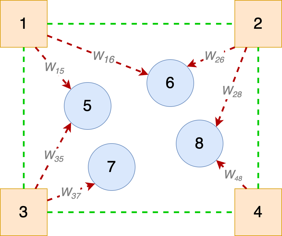
(a)

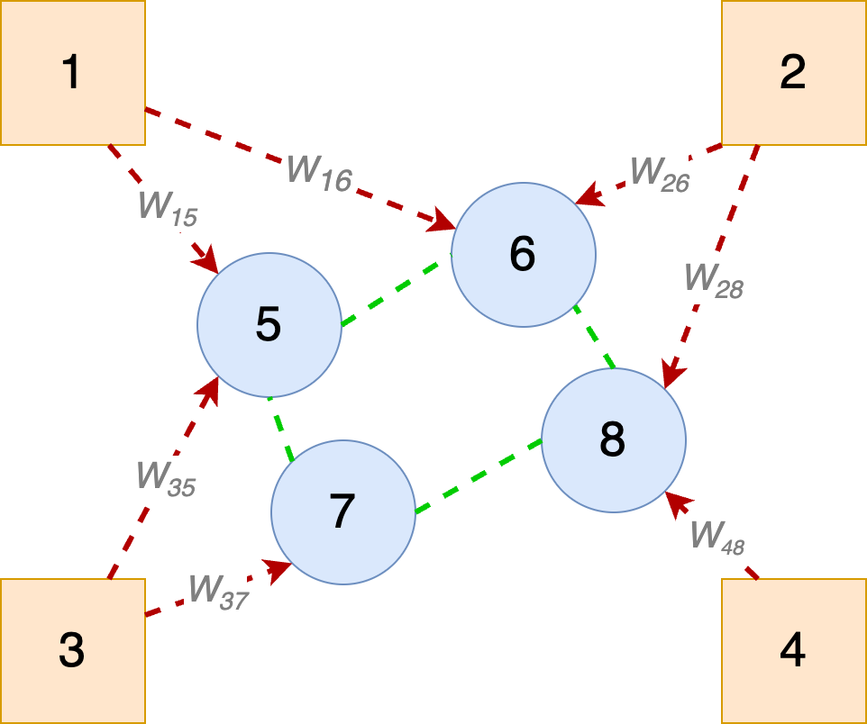
(b)

Fig. 1: Illustrations of mixed graphs for joint interpolation / denoising. Pixels 5,6,7,8 are interpolated using pixels 1,2,3,4. Directed edges for interpolation are shown as red dashed arrows, while undirected edges for denoising are shown as green dashed lines. (a) corresponds to corollary 1 where input pixels are denoised before interpolation. (b) corresponds to corollary 2 where interpolated pixels are denoised after interpolation.

4.1 Joint Formulation with Separable Solution

Denote by ${\mathbf{A}}\in\mathbb{R}^{(M+N)\times(M+N)}$ in the form (11) an adjacency matrix of a directed graph ${\mathcal{G}}^{d}$ connecting $M$ original pixels to $N$ new pixels, corresponding to an interpolator ${\boldsymbol{\Theta}}$. Further, denote by ${\mathbf{L}}\in\mathbb{R}^{M\times M}$ a graph Laplacian matrix for an undirected graph ${\mathcal{G}}^{u}$ inter-connecting the $M$ noisy original pixels, corresponding to a denoiser ${\boldsymbol{\Psi}}$. One direct formulation for joint denoising / interpolation is to simply combine terms in MAP objectives (4) and (12) as

$$\min_{{\mathbf{x}}}\|{\mathbf{y}}-{\mathbf{H}}{\mathbf{x}}\|^{2}_{2}+\gamma\|{\mathbf{H}}({\mathbf{x}}-{\mathbf{A}}{\mathbf{x}})\|^{2}_{2}+\mu({\mathbf{H}}{\mathbf{x}})^{\top}{\mathbf{L}}({\mathbf{H}}{\mathbf{x}}).$$ (34)

In words, (34) states that sought signal ${\mathbf{x}}$ should be smooth w.r.t. two graphs ${\mathcal{G}}^{d}$ and ${\mathcal{G}}^{u}$: i) ${\mathbf{x}}$ should be similar to its shifted version ${\mathbf{A}}{\mathbf{x}}$ where ${\mathbf{A}}$ is an adjacency matrix for a directed graph ${\mathcal{G}}^{d}$, and ii) original pixels ${\mathbf{H}}{\mathbf{x}}$ should be smooth w.r.t. to an undirected graph ${\mathcal{G}}^{u}$ defined by ${\mathbf{L}}$. We show that the optimal solution to the posed MAP problem (34) takes a particular form.

Corollary 1.

(34) has a separable solution.

Proof.

Optimization (34) is an unconstrained convex QP problem. Taking the derivative w.r.t. ${\mathbf{x}}$ and setting it to $0$, we get

$$\left({\mathbf{H}}^{\top}{\mathbf{H}}+\gamma\left(({\mathbf{I}}-{\mathbf{A}})^{\top}{\mathbf{H}}^{\top}{\mathbf{H}}({\mathbf{I}}-{\mathbf{A}})\right)+\mu{\mathbf{H}}^{\top}{\mathbf{L}}{\mathbf{H}}\right){\mathbf{x}}^{*}={\mathbf{H}}^{\top}{\mathbf{y}}.$$ (35)

Denote by ${\mathbf{C}}$ the coefficient matrix on the left-hand side. Given ${\mathbf{H}}=[{\mathbf{I}}_{M}~{}{\mathbf{0}}_{M,N}]$, ${\mathbf{H}}^{\top}{\mathbf{L}}{\mathbf{H}}$ has nonzero term ${\mathbf{L}}$ only in the upper-left sub-matrix. Given (16), ${\mathbf{C}}$ differs only in the upper-left block, i.e.,

$${\mathbf{C}}=\left[\begin{array}[]{cc}(\gamma+1){\mathbf{I}}_{M}+\mu{\mathbf{L}}&-\gamma{\mathbf{A}}_{M,N}\\ -\gamma{\mathbf{A}}_{N,M}&\gamma{\mathbf{A}}^{2}_{N,N}\end{array}\right].$$ (38)

Using the matrix inverse formula (21), we can first write block $\dot{{\mathbf{P}}}=(\dot{{\mathbf{A}}}-\dot{{\mathbf{B}}}\dot{{\mathbf{D}}}^{-1}\dot{{\mathbf{C}}})^{-1}$ as:

$$\dot{{\mathbf{P}}} =\left((\gamma+1){\mathbf{I}}_{M}+\mu{\mathbf{L}}-(-\gamma{\mathbf{A}}_{M,N})(\gamma{\mathbf{A}}_{N,N}^{2})^{-1}(-\gamma{\mathbf{A}}_{N,M})\right)^{-1}$$

$$=\left((\gamma+1){\mathbf{I}}_{M}+\mu{\mathbf{L}}-\gamma{\mathbf{I}}_{M}\right)^{-1}=({\mathbf{I}}_{M}+\mu{\mathbf{L}})^{-1}.$$ (39)

Thus, the solution ${\mathbf{x}}^{*}$ for optimization (35) is

$${\mathbf{x}}^{*} ={\mathbf{C}}^{-1}{\mathbf{H}}^{\top}{\mathbf{y}}$$

$$=\left[\begin{array}[]{c}({\mathbf{I}}_{M}+\mu{\mathbf{L}})^{-1}\\ -(\gamma{\mathbf{A}}_{N,N}^{2})^{-1}(-\gamma{\mathbf{A}}_{N,M})({\mathbf{I}}_{M}+\mu{\mathbf{L}})^{-1}\end{array}\right]$$ (42)

$$=\left[\begin{array}[]{c}({\mathbf{I}}_{M}+\mu{\mathbf{L}})^{-1}\\ {\mathbf{A}}_{M,N}^{-1}({\mathbf{I}}_{M}+\mu{\mathbf{L}})^{-1}\end{array}\right]=\left[\begin{array}[]{c}{\boldsymbol{\Psi}}\\ {\boldsymbol{\Theta}}\,{\boldsymbol{\Psi}}\end{array}\right]{\mathbf{y}},$$ (47)

where ${\boldsymbol{\Psi}}=\left({\mathbf{I}}_{M}+\mu{\mathbf{L}}\right)^{-1}$ is the denoiser, and ${\boldsymbol{\Theta}}={\mathbf{A}}_{M,N}^{-1}$ is the interpolator. We see that solution (47) to optimization (34) is entirely separable: input ${\mathbf{y}}$ first undergoes denoising via original denoiser ${\boldsymbol{\Psi}}$, then subsequently interpolation via original interpolator ${\boldsymbol{\Theta}}$. ∎

4.2 Joint Formulation with Non-separable Solution

Next, we consider a scenario where we introduce a GLR smoothness prior [10] for the $N$ interpolated pixels instead of a smoothness prior for the $M$ original pixels in (34), resulting in

$$\min_{{\mathbf{x}}} \|{\mathbf{y}}-{\mathbf{H}}{\mathbf{x}}\|^{2}_{2}+\gamma\|{\mathbf{H}}({\mathbf{x}}-{\mathbf{A}}{\mathbf{x}})\|^{2}_{2}+\kappa({\mathbf{G}}{\mathbf{x}})^{\top}\bar{{\mathbf{L}}}({\mathbf{G}}{\mathbf{x}}),$$ (48)

where ${\mathbf{G}}=[{\mathbf{0}}_{N,M}\;{\mathbf{I}}_{N}]$ selects only the $N$ new pixels from signal ${\mathbf{x}}$, and $\bar{{\mathbf{L}}}\in\mathbb{R}^{N\times N}$ denotes a graph Laplacian matrix for an undirected graph $\bar{{\mathcal{G}}}^{u}$ connecting the interpolated pixels.

Corollary 2.

(48) has a non-separable solution.

Proof.

(48) is convex, quadratic and differentiable. The optimal solution ${\mathbf{x}}^{*}$ can be computed via a system of linear equations,

$$\left({\mathbf{H}}^{\top}{\mathbf{H}}+\gamma\left(({\mathbf{I}}-{\mathbf{A}})^{\top}{\mathbf{H}}^{\top}{\mathbf{H}}({\mathbf{I}}-{\mathbf{A}})\right)+{\mathcal{L}}\right){\mathbf{x}}^{*}={\mathbf{H}}^{\top}{\mathbf{y}},$$ (49)

where ${\mathcal{L}}=\kappa{\mathbf{G}}^{\top}\bar{{\mathbf{L}}}{\mathbf{G}}$ and is block-diagonal, i.e.,

$${\mathcal{L}}=\left[\begin{array}[]{cc}{\mathbf{0}}_{M}&{\mathbf{0}}_{M,N}\\ {\mathbf{0}}_{N,M}&\kappa\bar{{\mathbf{L}}}\end{array}\right].$$ (52)

A similar derivation shows that coefficient matrix ${\mathbf{C}}$ changes from (38) to

$${\mathbf{C}}=\left[\begin{array}[]{cc}(\gamma+1){\mathbf{I}}_{M}&-\gamma{\mathbf{A}}_{M,N}\\ -\gamma{\mathbf{A}}_{N,M}&\gamma{\mathbf{A}}^{2}_{N,N}+\kappa\bar{{\mathbf{L}}}\end{array}\right].$$ (55)

Using again the matrix inverse formula (21), we first write block $\dot{{\mathbf{P}}}=(\dot{{\mathbf{A}}}-\dot{{\mathbf{B}}}\dot{{\mathbf{D}}}^{-1}\dot{{\mathbf{C}}})^{-1}$ as

$$\dot{{\mathbf{P}}} =\left((\gamma+1){\mathbf{I}}_{M}-(-\gamma{\mathbf{A}}_{M,N})(\gamma{\mathbf{A}}_{N,N}^{2}+\kappa\bar{{\mathbf{L}}})^{-1}(-\gamma{\mathbf{A}}_{N,M})\right)^{-1}$$

$$=\left((\gamma+1){\mathbf{I}}_{M}-\gamma^{2}{\mathbf{A}}_{M,N}(\gamma{\mathbf{A}}_{N,N}^{2}+\kappa\bar{{\mathbf{L}}})^{-1}{\mathbf{A}}_{N,M}\right)^{-1}.$$ (56)

The solution for ${\mathbf{x}}^{*}$ in (49) is

$${\mathbf{x}}^{*} ={\mathbf{C}}^{-1}{\mathbf{H}}^{\top}{\mathbf{y}}=\left[\begin{array}[]{c}\dot{{\mathbf{P}}}\\ -(\gamma{\mathbf{A}}_{N,N}^{2}+\kappa\bar{{\mathbf{L}}})^{-1}(-\gamma{\mathbf{A}}_{N,M})\dot{{\mathbf{P}}}\end{array}\right]$$ (59)

$$=\left[\begin{array}[]{c}\dot{{\mathbf{P}}}\\ \gamma(\gamma{\mathbf{A}}_{N,N}^{2}+\kappa\bar{{\mathbf{L}}})^{-1}{\mathbf{A}}_{N,M}\dot{{\mathbf{P}}}\end{array}\right]=\left[\begin{array}[]{c}{\boldsymbol{\Psi}}^{*}\\ {\boldsymbol{\Theta}}^{*}\,{\boldsymbol{\Psi}}^{*}\end{array}\right]{\mathbf{y}},$$ (64)

where ${\boldsymbol{\Psi}}^{*}=\dot{{\mathbf{P}}}$ is a derived denoiser for original pixels, and ${\boldsymbol{\Theta}}^{*}=\gamma(\gamma{\mathbf{A}}_{N,N}^{2}+\kappa\bar{{\mathbf{L}}})^{-1}{\mathbf{A}}_{N,M}$ is an augmented interpolator. Since ${\boldsymbol{\Theta}}^{*}{\boldsymbol{\Psi}}^{*}\neq\bar{{\boldsymbol{\Psi}}}{\boldsymbol{\Theta}}$, the solution to (48) is not separable. ∎

Remarks: ${\boldsymbol{\Psi}}^{*}$ is a denoiser because it denoises $M$ original pixels. ${\boldsymbol{\Theta}}^{*}$ is an interpolator because it operates on the $M$ denoised original pixels and outputs $N$ interpolated pixels. ${\boldsymbol{\Psi}}^{*}$ and ${\boldsymbol{\Theta}}^{*}$ are analytically derived denoising and interpolation operators that are computable functions of original directed graph adjacency matrix ${\mathbf{A}}$ for interpolation and undirected graph Laplacian $\bar{{\mathbf{L}}}$ for denoising. We show next that using the derived operators for joint interpolation / denoising can result in performance better than separate schemes.

5 Experiments

5.1 Experimental setup

Experiments were conducted to test our derived operators in (64) for joint denoising / interpolation (denoted by joint) compared to original sequential operations (denoted by sequential) in the non-separable case. For denoisers, we employed Gaussian filter [12], bilateral filter (BF) [14] and nonlocal means (NLM) [17, 18]. For interpolators, we used linear operators for image rotation and warping using Homography transform. The output images were evaluated using signal-to-noise ratio (PSNR). Popular $512\times 512$ grayscale images, Lena and peppers, were used for rotation and warping, respectively. The experiments were run in Matlab R2022a. Gaussian noise of different variances were added to the images.

The joint denoising / interpolation operation was performed on $10\times 10$ output patches. The size and location of the input patch from which the output patch is generated depend on the interpolation operation and the output location. To ensure that the number of input pixels is equal to the output pixels (i.e., $M=N$), we interpolated dummy pixels by adding rows to ${\boldsymbol{\Theta}}$. It is also important to ensure that ${\boldsymbol{\Theta}}$ is full rank (thus invertible) when adding new rows.

To ensure denoiser ${\boldsymbol{\Psi}}$ is non-expansive, symmetric and PD according to Theorem 1, we ran the Sinkhorn-Knopp procedure [19] for an input linear denoiser with non-negative entries and independent rows, so that matrix ${\boldsymbol{\Psi}}$ was double stochastic, and thus its eigenvalues satisfied $|\lambda_{i}|\leq 1,\forall i$. Note that for a chosen interpolation operation, ${\boldsymbol{\Theta}}$ changed from patch to patch, and so the denoiser needed to adapt to the input and output dimensions when using the Gaussian filter. For BF, and NLM, the denoiser itself changed from patch to patch. To solve (49) in each iteration, pcg function in MATLAB implementing a version of conjugate gradient [20] was used.

Image rotation was performed at 20 degrees anti-clockwise, and for image warping a homography matrix of [1, 0.2, 0; 0.1, 1, 0; 0, 0, 1] was used. For the experiments with Gaussian filter and BF, the hyperparameters were selected as $\mu=0.3$, $\gamma=0.5$, $\kappa=0.3$. For Gaussian denoiser, a variance of $0.3$ was used, and for BF, variance of $0.3$ was used for both spatial and range kernels. For experiments with NLM, $\gamma=0.6$, $\kappa=0.2$, while $\mu$ was kept the same. The patch size for NLM was $3\times 3$ and the search window size was $9\times 9$.

5.2 Experimental Results

Fig. 2 show that joint performed better than sequential in general. While the performance of both schemes degraded as noise variance increased, the performance of sequential degraded faster than joint. In the experiment with image rotation and Bilateral denoiser, we observe a maximum PSNR gain of $1.35$dB, and when NLM was used, the maximum gain was $0.77$dB. Note that we have reported results for NLM over a larger range of noise variance, because NLM generally produced high-quality output, and thus the PSNR difference between joint and sequential is small at low noise levels. For image warping, the maximum gains were $1.05$dB and $1.14$dB for bilateral and Gaussian denoisers, respectively.

Fig. 2: Plots comparing the performance of joint vs sequential over a range of noise variance using 4 combinations of interpolators and denoisers. (a) Image rotation + Bilateral denoiser. (b) Image rotation + Non-Local Means denoiser. (c) Image warping + Bilateral denoiser. (d) Image warping + Gaussian denoiser.

6 Conclusion

We presented two theorems, under mild conditions, connecting any linear denoiser / interpolator to optimal graph filter regularized using an undirected / directed graph. The theorems demonstrate the generality of graph filters and provide graph interpretations for common linear denoisers / interpolators. Using the two theorems, we examine scenarios of joint denoising / interpolation where the optimal solution can be separable or non-separable. In the later case, analytically derived denoiser / interpolator can be computed as functions of original denoiser and interpolator. We demonstrate that using these computed operators resulted in noticeable performance gain over seperate schemes in a range of joint denoising / interpolation settings.

References

- [1] Henrique S Malvar, Li-wei He, and Ross Cutler, “High-quality linear interpolation for demosaicing of bayer-patterned color images,” in IEEE International Conference on Acoustics, Speech, and Signal Processing. IEEE, 2004, vol. 3, pp. iii–485.
- [2] Daniele Menon and Giancarlo Calvagno, “Color image demosaicking: An overview,” Signal Processing: Image Communication, vol. 26, no. 8-9, pp. 518–533, 2011.
- [3] Zhucun Xue, Nan Xue, Gui-Song Xia, and Weiming Shen, “Learning to calibrate straight lines for fisheye image rectification,” in Proceedings of the IEEE/CVF Conference on Computer Vision and Pattern Recognition, 2019, pp. 1643–1651.
- [4] Kai Zhang, Wangmeng Zuo, Yunjin Chen, Deyu Meng, and Lei Zhang, “Beyond a Gaussian denoiser: Residual learning of deep CNN for image denoising,” IEEE Transactions on Image Processing, vol. 26, no. 7, pp. 3142–3155, 2017.
- [5] Wenzhu Xing and Karen Egiazarian, “End-to-end learning for joint image demosaicing, denoising and super-resolution,” in Proceedings of the IEEE/CVF Conference on Computer Vision and Pattern Recognition, 2021, pp. 3507–3516.
- [6] Filippos Kokkinos and Stamatios Lefkimmiatis, “Iterative joint image demosaicking and denoising using a residual denoising network,” IEEE Transactions on Image Processing, vol. 28, no. 8, pp. 4177–4188, 2019.
- [7] A. Ortega, P. Frossard, J. Kovacević, J. M. F. Moura, and P. Vandergheynst, “Graph signal processing: Overview, challenges, and applications,” in Proceedings of the IEEE, May 2018, vol. 106, no.5, pp. 808–828.
- [8] G. Cheung, E. Magli, Y. Tanaka, and M. Ng, “Graph spectral image processing,” in Proceedings of the IEEE, May 2018, vol. 106, no.5, pp. 907–930.
- [9] Stanley H. Chan, “Performance analysis of plug-and-play ADMM: A graph signal processing perspective,” IEEE Transactions on Computational Imaging, vol. 5, no. 2, pp. 274–286, 2019.
- [10] J. Pang and G. Cheung, “Graph Laplacian regularization for inverse imaging: Analysis in the continuous domain,” in IEEE Transactions on Image Processing, April 2017, vol. 26, no.4, pp. 1770–1785.
- [11] Y. Romano, M. Elad, and P. Milanfar, “The little engine that could: Regularization by denoising (red),” in SIAM Journal on Imaging Sciences, 2017, vol. 10, no.4, pp. 1804–1844.
- [12] P. Milanfar, “A tour of modern image filtering,” in IEEE Signal Processing Magazine, January 2013, vol. 30, no.1, pp. 106–128.
- [13] Xianming Liu, Gene Cheung, Xiaolin Wu, and Debin Zhao, “Random walk graph Laplacian-based smoothness prior for soft decoding of JPEG images,” IEEE Transactions on Image Processing, vol. 26, no. 2, pp. 509–524, 2017.
- [14] C. Tomasi and R. Manduchi, “Bilateral filtering for gray and color images,” in Proceedings of the IEEE International Conference on Computer Vision, Bombay, India, 1998.
- [15] Akshay Gadde, Sunil K Narang, and Antonio Ortega, “Bilateral filter: Graph spectral interpretation and extensions,” in IEEE International Conference on Image Processing, 2013, pp. 1222–1226.
- [16] Dennis S Bernstein, Matrix mathematics: theory, facts, and formulas, Princeton University Press, 2009.
- [17] Antoni Buades, Bartomeu Coll, and Jean-Michel Morel, “Non-local means denoising,” Image Processing On Line, vol. 1, pp. 208–212, 2011.
- [18] A. Buades, B. Coll, and J. Morel, “A non-local algorithm for image denoising,” in IEEE International Conference on Computer Vision and Pattern Recognition, San Diego, CA, June 2005.
- [19] Philip A Knight, “The sinkhorn–knopp algorithm: convergence and applications,” SIAM Journal on Matrix Analysis and Applications, vol. 30, no. 1, pp. 261–275, 2008.
- [20] Martin Fodslette Moller, “A scaled conjugate gradient algorithm for fast supervised learning,” Neural Networks, vol. 6, no. 4, pp. 525–533, 1993.