Machine-Learning Enhanced Photometric Analysis of the Extremely Bright GRB 210822A

Abstract

We present analytical and numerical models of the bright long GRB 210822A at $z=1.736$. The intrinsic extreme brightness exhibited in the optical, which is very similar to other bright GRBs (e.g., GRBs 080319B, 130427A, 160625A 190114C, and 221009A), makes GRB 210822A an ideal case for studying the evolution of this particular kind of GRB. We use optical data from the RATIR instrument starting at $T+315.9$ s, with publicly available optical data from other ground-based observatories, as well as Swift/UVOT, and X-ray data from the Swift/XRT instrument. The temporal profiles and spectral properties during the late stages align consistently with the conventional forward shock model, complemented by a reverse shock element that dominates optical emissions during the initial phases ($T<300$ s). Furthermore, we observe a break at $T=80000$ s that we interpreted as evidence of a jet break, which constrains the opening angle to be about $\theta_{\mathrm{j}}=(3-5)$ degrees. Finally, we apply a machine-learning technique to model the multi-wavelength light curve of GRB 210822A using the afterglowpy library. We estimate the angle of sight $\theta_{obs}=(6.4\pm 0.1)\times 10^{-1}$ degrees, the energy $E_{0}=(7.9\pm 1.6)\times 10^{53}$ ergs, the electron index $p=2.54\pm 0.10$, the thermal energy fraction in electrons $\epsilon_{\mathrm{e}}=(4.63\pm 0.91)\times 10^{-5}$ and in the magnetic field $\epsilon_{\mathrm{B}}=(8.66\pm 1.01)\times 10^{-6}$, the efficiency $\chi=0.89\pm 0.01$, and the density of the surrounding medium $n_{\mathrm{0}}=0.85\pm 0.01~{}cm^{-3}$.

1 Introduction

Gamma-ray bursts (GRBs) are the brightest events in the universe (Kumar & Zhang, 2015). It is possible to associate the duration of the event with the progenitors using the parameter $T_{90}$. Currently, two types of GRBs are known (Kouveliotou et al., 1993). Short GRBs (SGRBs), which are thought to be produced by the merger of two compact objects, typically have $T_{90}\lesssim 2$ s and a harder spectrum (Lee & Ramirez-Ruiz, 2007; Berger, 2014), whereas long GRBs (LGRBs) typically have a $T_{90}\gtrsim 2$ s and a softer spectrum, and are associated with the death of a massive star (Kouveliotou et al., 1993; Woosley, 1993; MacFadyen & Woosley, 1999; Hjorth et al., 2003; Oates, 2023). Nevertheless, in recent years, events with the characteristics of both populations have been reported (see e.g. GRB 200826A (Ahumada et al., 2021; Zhang et al., 2021), GRB 211211A (Rastinejad et al., 2022; Troja et al., 2022), GRB 210704A (Becerra et al., 2023a) and GRB 230307A (Levan et al., 2023; Yang et al., 2023)).

The fireball model (Mészáros & Rees, 1997; Granot & Sari, 2002; Kumar & Zhang, 2015) is the most successful theory for interpreting the electromagnetic radiation of GRBs. The model explains the observed prompt (gamma-ray) emission by internal shocks in the jet driven by a central engine (Sari & Piran, 1997) and the late emission or afterglow by the existence of an external shock between the outflow and the circumburst medium (e.g., Sari et al., 1998; Granot & Sari, 2002). The radiation process that dominates the afterglow is synchrotron emission, produced by relativistic electrons that are continuously accelerated by an ongoing shock interacting with the surrounding medium. This blast wave produces a forward shock that propagates into the surrounding medium and a reverse shock that propagates inward through the relativistic shell (Sari et al., 1998; Sari & Piran, 1999).

For later times, a similar evolution of the X-ray and optical emission would be expected for a GRB (Kumar & Zhang, 2015; Zhang et al., 2006). Nevertheless, there are numerous features that appear in optical that are not seen simultaneously in X-rays, such as the reverse shock component and early rebrightening (see e.g. Li et al., 2012; Becerra et al., 2023b). These features can suggest different characteristics, such as: the GRB origin being different, they are in a different spectral segment (Granot & Sari, 2002), are produced by different components, or are produced in a more complex environment (see e.g. Gao & Mészáros, 2015).

Bright GRBs permit follow-up for a longer period of time (see e.g. O’Connor et al., 2023; Becerra et al., 2023a, 2019a), leading to a better understanding of their progenitors and circumburst environments. Given that only about 40% of these phenomena have a well-determined distance (Evans et al., 2007, 2009), the study of particularly bright GRBs with known distances is extremely valuable because they allow us to explore in more detail the morphology and structure of the jet (see e.g. Gill et al., 2019).

Here, we present photometric observations of the long GRB 210822A in the optical, UV, and X-rays during the afterglow phase and compare them with the detailed predictions of the fireball model.

Our paper is organised as follows. In Section 2, we present observations with Swift, RATIR, Katzman Automatic Imaging Telescope (KAIT), the Nordic Optical Telescope (NOT), and other ground-based telescopes. In Section 3 we present our analysis. We discuss the nature of the GRB 210822A and its interpretation within the context of the current fireball model, and we conduct a comparative analysis of our photometry with other events and deduce the physical parameters that could describe this explosion in Section 4. Finally, we provide a summary of our results in Section 5.

2 Observations

2.1 High-energy

The Swift/BAT instrument triggered on GRB 210822A at $T=$ 2021 August 22 09:18:18 UTC (Page et al., 2021). The Swift/BAT on-board location was 20:17:50.7 +05:15:54.9 J2000, with an uncertainty of 3.0 arcmin (radius, 90% containment, including systematic uncertainty). The Swift/BAT mask-weighted light curve showed a multi-peaked structure that started and peaked at the time of trigger ($T$). The main pulse structure ended at about $T+20$ s, followed by a long tail that lasted until about $T+400$  s. The duration of GRB 210822A (15-350 keV) was $T_{90}=185.8\pm 46.6$ seconds, making it a long GRB, with an estimated fluence of 2.0$\pm$0.04$\times 10^{-6}$ erg cm^-2 in the 15–150 keV band (Lien et al., 2021). We investigate the similarities of GRB 210822A with previous Swift/BAT events (Evans et al., 2007, 2009), in order to identify other similar phenomena using a machine learning approach. The method and results are presented in Section 4.2.1.

The Konus-Wind instrument reported observations starting at about $T-1$ s and with a total duration of about 12 s. According to Frederiks et al. (2021), the burst had a fluence of $1.20\pm 0.11\times~{}10^{-4}$ erg cm^-2 and a 64 ms peak flux, measured from $T+0.320$ s, of $3.25\pm 0.28\times~{}10^{-5}$ erg cm^-1 (both in the 20 keV to 10 MeV energy range).

The Swift/X-ray Telescope (XRT) instrument started observing the field at $T+74.6$ s and found an uncatalogued X-ray source at 20:17:45.01 +05:17:00.6 J2000 with an uncertainty of 2.0 arcsec (radius, 90% containment). Its location, only 145 arcsec from the Swift/BAT on board position (Page et al., 2021), was well inside the Swift/BAT error circle.

Finally, the Swift/Ultra-violet Optical Telescope (UVOT) instrument began settled observations of the field of GRB 210822A at $T+85$ s, detecting a fading source consistent with the Swift/XRT position (Siegel et al., 2021). Swift/UVOT took a finding chart exposure of 250 seconds with the $u$ filter starting at $T+295$ s (Page et al., 2021). The afterglow candidate was found in the initial data products in all filters.

2.2 Optical

2.2.1 RATIR

The Reionization and Transients InfraRed camera (RATIR) is a four-channel simultaneous optical and near-infrared imager. It was mounted on the 1.5 meters Harold L. Johnson Telescope at the Observatorio Astronómico Nacional in Sierra San Pedro Mártir in Baja California, Mexico, until summer 2022. RATIR autonomously responded to GRB triggers from the Swift satellite and obtained simultaneous photometry in $riZJ$ or $riYH$ bands (Butler et al., 2012; Watson et al., 2012; Littlejohns et al., 2015; Becerra et al., 2017). The reduction pipeline performed bias subtraction and flat field correction, followed by astrometric calibration using astrometry software (Lang et al., 2010), iterative sky subtraction, co-addition using SWARP, and source detection using sextractor (Bertin & Arnouts, 1996; Becerra et al., 2017; Pereyra et al., 2022). We calibrated against the U.S. Naval Observatory B1 catalogue (USNO-B1) (Monet et al., 2003) and the Two Micron All-Sky Survey (2MASS) (Skrutskie et al., 2006).

RATIR observed the field of GRB 210822A from 2021 August 22 09:19:30 to 09:48:54 UTC (from $T+0.02$ to $T+0.49$ hours after the BAT trigger), obtaining a total of 0.19 hours of exposure in the $r$ and $i$ bands (Butler et al., 2021). RATIR obtained individual frames of 80 s of exposure time. RATIR photometry is presented in Table 1, as magnitudes in the AB system and without correction for the Milky Way extinction in the direction of the burst, and shown in Figure 1.

Table 1: Photometry of GRB 210822A.

Data from this work (RATIR data)
Time [s]	Exp [s]	Filter	Magnitude	Instrument
1199.2	80	r	15.15 $\pm$ 0.01	RATIR
1604.0	80	r	15.53 $\pm$ 0.01	RATIR
1709.0	80	r	15.60 $\pm$ 0.01	RATIR
315.9	80	i	13.17 $\pm$ 0.00	RATIR
416.9	80	i	13.78 $\pm$ 0.00	RATIR
516.3	80	i	14.15 $\pm$ 0.00	RATIR
609.8	80	i	14.20 $\pm$ 0.00	RATIR
708.9	80	i	14.47 $\pm$ 0.00	RATIR
904.1	80	i	15.00 $\pm$ 0.00	RATIR
997.9	80	i	14.93 $\pm$ 0.01	RATIR
1098.6	80	i	15.03 $\pm$ 0.01	RATIR
1398.6	80	i	15.34 $\pm$ 0.01	RATIR
1604.0	80	i	15.79 $\pm$ 0.01	RATIR
1709.0	80	i	15.86 $\pm$ 0.01	RATIR
1803.8	80	i	15.72 $\pm$ 0.01	RATIR

GCN data from optical ground-based facilities
Time [s]	Exp [s]	Filter	Magnitude	Instrument	Reference
114.0	20.0	w	11.40 $\pm$ $\cdot\cdot\cdot$	KAIT	Zheng et al. (2021)
2690.0	20.0	w	16.10 $\pm$ $\cdot\cdot\cdot$	KAIT	Zheng et al. (2021)
20424.9	1500.0	r	18.53 $\pm$ 0.06	NANSHAN	Fu et al. (2021)
23760.0	10000.0	V	18.88 $\pm$ 0.08	NANSHAN	Fu et al. (2021)
31262.9	3920	R	18.63 $\pm$ 0.03	TSHAO	Belkin et al. (2021a)
37400.8	420.0	i	18.56 $\pm$ 0.14	CAHA	Kann et al. (2021)
50004.0	360.0	r	19.71 $\pm$ 0.02	NOT	Zhu et al. (2021)
58665.6	2760.0	R	20.10 $\pm$ 0.30	Abbey Ridge	Romanov & Lane (2021)
63822.0	600.0	i’	19.92 $\pm$ 0.05	GROND	Nicuesa Guelbenzu et al. (2021)
63822.0	600.0	g’	20.37 $\pm$ 0.09	GROND	Nicuesa Guelbenzu et al. (2021)
63822.0	600	r’	20.10 $\pm$ 0.05	GROND	Nicuesa Guelbenzu et al. (2021)
201347.4	3180.0	R	21.60 $\pm$ 0.26	TSHAO	Belkin et al. (2021b)

2.2.2 Other optical ground-based facilities

We complement RATIR photometry with data from other optical telescopes from the GCN/TAN circulars, such as the 0.76 m Katzman Automatic Imaging Telescope (KAIT) (Zheng et al., 2021), the NEXT-0.6 m telescope (NANSHAN) (Fu et al., 2021), the Nordic Optical Telescope (NOT) (Zhu et al., 2021), the Gamma-Ray Burst Optical/Near-Infrared Detector (GROND) (Nicuesa Guelbenzu et al., 2021), the Tian Shan Astronomical Observatory (TSHAO) (Belkin et al., 2021a), the Calar Alto Astronomical Observatory (CAHA) (Kann et al., 2021) and the 0.35 m telescope at the Abbey Ridge Observatory (Romanov & Lane, 2021). This photometry is listed in Table 1 and shown in Figure 1.

Zhu et al. (2021) estimated a redshift of $z=1.736$ for the GRB 210822A using spectroscopic observations with NOT in the $3700-9500$ Å range that showed a continuum with absorption characteristics from the Fe ii, Mg ii, Mg i and Al iii lines.

Additionally, Page et al. (2021) and Siegel et al. (2021) reported a reddening of $E(B-V)=0.162$ in the direction of the burst. We calculate the extinction $A_{r}$, adopting the relationship $A_{V}=3.1\times$$E(B-V)$ (Schlegel et al., 1998) and $A_{r}/A_{V}\approx 0.9$ (Gordon et al., 2003).

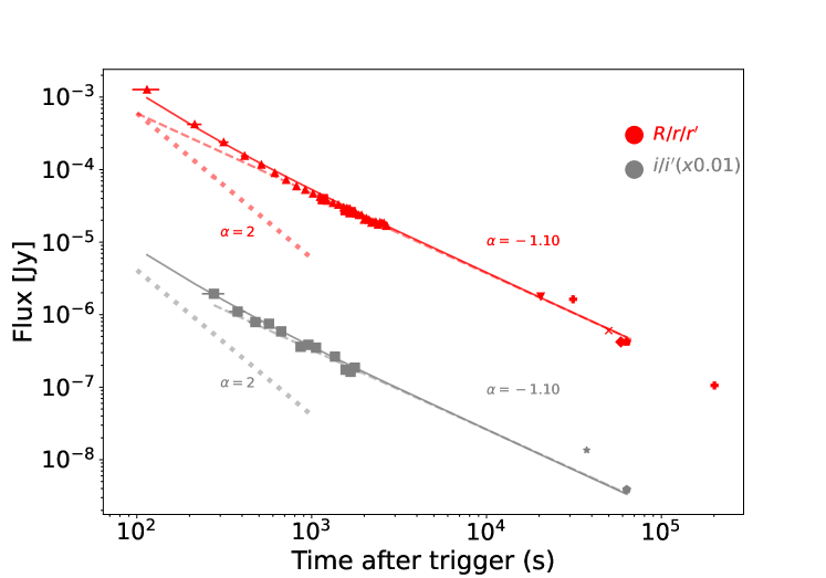
Figure 1: Optical light curves of GRB 210822A. The red and gray symbols correspond to data in the r and i bands, respectively. Different symbols indicate data from RATIR (squares), KAIT (upward triangles), GROND (pentagons), NOT (crosses), TSHAO (pluses), CAHA (stars), and Abbey Ridge (diamonds). We illustrate the reverse shock (dotted line) and forward shock (dashed line) components that best fit the optical observations, as well as the sum of both (continuous line), for both the $r$ and $i$ bands. The temporal slopes that better describe the forward shock emission during the afterglow are also shown. The evolution of the light curve after $T+80000$ s is discussed in Section 4.1

3 Temporal and spectral analysis

In the framework of the fireball model, the afterglow phase is explained as synchrotron radiation from a population of accelerated electrons $N$ with a power-law energy distribution $N(E)\propto E^{-p}$, where $E$ and $p$ are the energy and index respectively. Typically, the observed flux density $F_{\nu}$ has a multisegmented power-law profile in both time $t$ and frequency $\nu$, denoted as $F_{\nu}\propto t^{-\alpha}\nu^{-\beta}$ (Sari et al., 1998; Granot & Sari, 2002).

3.1 Temporal Analysis

Figure 1 shows the best fit to our optical photometry. Our data, in both filters, are well-modelled by one single power law segment for times between $T+300$ s a $T+80000$  with a power law $F_{\nu}\propto t^{-1.10\pm 0.01}$. This finding is in good agreement with the average decay index observed in large samples of GRB afterglows (Liang et al., 2010; Oates et al., 2009) and is consistent with an isotropic forward shock in a constant-density medium. However, we note that for early times our photometry in the $r$ band is better fit when a reverse-shock component is considered. (The data in the $i$ band do not extend to such early times, but are also consistent with a reverse shock.) For a detailed discussion on the temporal evolution of the afterglow we refer to Sections 3.1.1 and 4.1.

3.1.1 Early Afterglow

Figure 1 shows the best fit to our photometry. Both optical filters are well-modelled by one single power law segment for times after $T+300$ s. We observe that for early times ($T<300$ s), the photometry in the $r$ band lies above our fit. To address this discrepancy, we fit these points independently using a distinct power law (depicted by the red dotted line in Figure 1). We consider a function $F_{\nu}\propto t^{-2}$ according to the anticipated decay pattern of a reverse shock component (Gao & Mészáros, 2015), obtaining a better match to our photometry. We interpret this feature as the signature of the reverse shock propagating in the inner shell of the relativistic jet present in GRB 210822A (Sari & Piran, 1999; Becerra et al., 2019a, b; Gomboc et al., 2009; Mészáros & Rees, 1999). The presence of a reverse shock suggests the presence of a matter-dominated shell, which implies a low level of magnetisation (Zhang & Kobayashi, 2005; Zhang & Yan, 2011; García-García et al., 2023).

3.2 Spectral Analysis

In order to complement our photometric analysis, we retrieved light curves and spectra from the UK Swift Science Data Centre (UKSSDC) online repository (Evans et al., 2009) in the range of 0.3–10 keV. We binned all data retrieved from Swift/XRT, for Window Timing and Photon Count modes independently (see Evans et al., 2007), considering groups of 3 consecutive exposures, which yields a variable size for the time bins. From $T+78$ s to $T+1300$ s, early times, bin sizes are around 1 to 7 s. The size bin increases significantly to tens or even hundreds of seconds for the late time observations, from $T+4500$ s to $T+502000$ s, where data are sparse.

The optical and X-ray data at $T+500$ and $T+43000$ s are well-fitted with a simple absorbed power law of slope $\beta=-0.77\pm 0.03$ (see Figure 2), which indicates that they belong to the same spectral segment. $F_{\nu}\propto\nu^{-0.77\pm 0.03}$ yields an electron index of $p=2.54\pm 0.10$ for GRB 210822A, and implies a value of $F_{\nu}\propto t^{-1.15\pm 0.06}$ that is consistent with the temporal decay found in Section 3.1. Compared to the expected afterglow spectrum detailed in Granot & Sari (2002), we identify this segment as the frequency interval where $\nu_{\mathrm{m}}<\nu_{\mathrm{opt}}<\nu_{X}<\nu_{c}$.

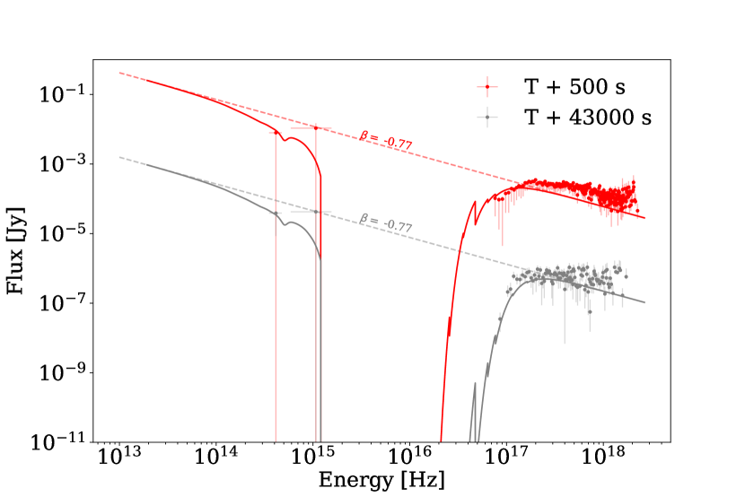
Figure 2: SED of GRB 210822A at $T+500~{}s$ (red) and $T+43000~{}s$ (gray). We use optical data from Table 1 and Swift/XRT data retrieved from the UKSSDC. We show the corresponding Xspec model (continuous lines), which considers the effects of reddening and absorption by the dust, as well as the linear fit (dashed lines).

Figure 2 also shows the fit of the model xspec that considers the effects of reddening and absorption by dust (Arnaud, 1996). We performed our analysis at $T+500$ s and $T+43000$ s to compare the evolution of the SED. We used a reddening of $E(B-V)=0.162$ (Page et al., 2021), a redshift of $z=1.786$ (Zhu et al., 2021), and a column density of $1.45\times 10^{21}$cm^-2 (Perri et al., 2021). We obtained reduced $\chi^{2}=3.07$ and $\chi^{2}=0.92$ with 698 and 300 degrees of freedom, at $T+500$ s and $T+43000$ s, respectively.

3.3 Machine Learning Method

Machine learning (ML) has found diverse applications within astrophysics, spanning from exoplanet identification (Malik et al., 2021) and galaxy categorisation (Ferreira et al., 2020) to supernova classification (Lochner et al., 2016), spectral modelling (Vogl et al., 2020), and gravitational wave detection (Ni, 2016). It is worth noting that the majority of these applications consider ML for classification purposes, with limited utilisation in modelling.

Based on the results obtained in the Section 3.2, we plot in Figure 3 the light curves in the $r$ and $i$ bands by scaling the optical flux to a common frequency of 1 keV, considering $\nu^{-0.77}$, and employ ML methodologies to build a predictive model for the afterglow of GRB 210822A.

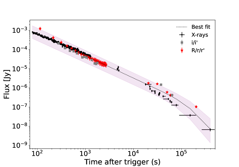
Figure 3: X-ray and optical light curves of GRB 210822A. Optical photometry is re-scaled to a common frequency of 1 keV by employing the scaling $\nu^{-0.77}$ obtained in Section 3.2. We illustrate the model of the light curve of GRB 210822A using ML (dashed black line) and the $1\sigma$ error region (shaded magenta area). The parameters of our best fit are listed in Table 2.

Details of this implementation are described in Appendix A. To effectively train and evaluate the ML model, we generate synthetic light curve data with the afterglowpy library (Ryan et al., 2020). This synthetic data set is then used to train the ML model built in the Keras and TensorFlow libraries, as referenced in Chollet (2015), which subsequently processes the actual observational photometric data from Table 1 to extract the parameters that align with the prediction of the model, introducing a novel and unprecedented approach in the field.

We created a diverse data set comprising 30,000 synthetic GRB light curve models. These models included values of random parameters within predefined ranges for the angle of view $\theta_{obs}$, the energy $E_{0}$, the opening angle $\theta_{\mathrm{j}}$, the electron index $p$, the thermal energy fraction in electrons $\epsilon_{\mathrm{e}}$ and in the magnetic field $\epsilon_{\mathrm{B}}$, efficiency $\chi$, and the density of the surrounding medium $n_{\mathrm{0}}$ (Sari et al., 1998; Granot & Sari, 2002). These parameters are listed in Appendix 5.

The trained ML model was evaluated with observed GRB data, corrected by Galactic extinction, producing the parameter estimates shown in Table 2. The results of the optimal parameters applied to afterglowpy can be seen in Figure 3.

Nevertheless, we note that a machine learning method such as the one employed in the fit presented in Figure  3, inherently selects a single set of parameters. The 1$\sigma$ error region is used to illustrate how well the best model fits the data, for the selected parameters (see details in Appendix A). As discussed by Garcia-Cifuentes et al. (2023a), in several adjustment methods, to find degeneracy in the parameters is not unusual. Such is the case of the relationship (scaling function) found between $E_{0}$, $n_{0}$ and $\epsilon_{\mathrm{B}}$ depending on the value of $p$, in the same spectral regime for the afterglow (van Eerten & MacFadyen, 2012; Granot, 2012; Garcia-Cifuentes et al., 2023a). Thus, the photometry of the GRBs can be reproduced by a range of values given their energy, density and microphysical parameters.

Parameter	Value $\pm$ Error
$\theta_{\mathrm{obs}}$	$(6.4\pm 0.1)\times 10^{-1}$ degrees
$E_{0}$	$(7.9\pm 1.6)\times 10^{53}$ ergs
$\theta_{\mathrm{j}}$	$(3.7\pm 0.5)$ degrees
$p$	$2.54\pm 0.10$
$\epsilon_{\mathrm{e}}$	$(4.63\pm 0.91)\times 10^{-5}$
$\epsilon_{\mathrm{B}}$	$(8.66\pm 1.01)\times 10^{-6}$
$\chi$	$0.89\pm 0.01$
$n_{\mathrm{0}}$	$(0.85\pm 0.01)$ cm-3

Table 2: Parameter Values and Errors

4 Discussion

4.1 Jet break

From Figure 3, we suggest the presence of a jet break between $T+80000$ s and $T+100000$ s (0.93–1.16 days). Considering this scenario, the opening angle for a constant density ISM depends on the jet break time as:

$$\theta_{\mathrm{j}} = 0.07\textrm{ rad}{\left(\frac{t_{\mathrm{break}}}{1\textrm{ day}}\right)}^{3/8}{\left(\frac{1+z}{2}\right)}^{-3/8}$$ (1)

$$\times \textrm{ }{\left(\frac{E_{\mathrm{K,iso}}}{10^{53}\textrm{ erg}}\right)}^{-1/8}{\left(\frac{n}{0.1\textrm{ cm}^{-3}}\right)}^{1/8}$$

where, $E_{\mathrm{K,iso}}$ is the isotropic kinetic energy of the blast wave and $n$ refers to the density of the circumburst medium (Wang et al., 2018). Assuming typical values of $n_{0}=0.85$ cm^-3 (see Section 3.3) and $E_{\mathrm{K,iso}}$=10⁵³–10⁵⁵ erg, and the measured value of $z=1.74$, we obtain an opening angle of the jet $\theta_{\mathrm{j}}=3$–$5\pm 0.5$ degrees. Our estimated opening angle is consistent with the lower limits for the existing GRB sample (Berger, 2014) and in good agreement with the value obtained from machine-learning modelling in Section 3.3.

4.2 GRB 210822A in the context of other GRBs

4.2.1 Gamma-rays

The classification of extremely bright LGRBs is essential for understanding their nature and origin. Recently, machine-learning methods provide a faster and more consistent way to classify transients and, specifically, GRBs, by automatically learning from the data and identifying patterns that may be difficult for humans to detect. Furthermore, machine-learning methods can handle large amounts of data, including multi-wavelength and multi-messenger observations, which are crucial for a comprehensive understanding of GRBs (see e.g. Jespersen et al., 2020; Garcia-Cifuentes et al., 2023b; Steinhardt et al., 2023).

Therefore, following the method presented by Garcia-Cifuentes et al. (2023b) using the ClassiPyGRB library. We analyse the Swift/BAT catalogue in order to find those GRBs whose gamma-ray emission measured by the Swift/BAT instrument are similar to GRB 210822A. This method is based on a popular non-linear dimensionality algorithm called t-SNE, which transforms high-dimensional data (in this case the Swift/BAT GRB light curves) into a 2-dimensional representation while preserving pairwise similarities (van der Maaten & Hinton, 2008). t-SNE ensures that the distances between points in the lower-dimensional representation reflect the similarities between patterns. For this work, we compare the discrete-time Fourier transform of the photometry in all bands of in the original Swift/BAT data. As demonstrated in Garcia-Cifuentes et al. (2023b), we reduce the noise impact by using the non-parametric approach presented by Sanchez-Alarcon & Ascasibar Sequeiros (2022) on 1451 Swift / BAT light curves. Then, we perform the following procedure:

• The light curves binned at $64$ ms are filtered using the $T_{100}$ duration presented in the Swift/BAT GRB catalogue.

• We normalised the light curves by the total fluence and ensured that every GRB has the same number of data points by padding zeros after the trigger in all bands.

• We perform a discrete-time Fourier transform (DTFT) on all events.

• We applied the t-SNE method to the Fourier Amplitude Spectrum for the entire sample.

In Figure 4 we show all Swift/BAT GRBs on the t-SNE map. In this lower-dimensional plane, points that are closer to each other have more similarities in their original data than points that are further apart. This means that t-SNE maps provides a visual representation of the whole dataset, where the relative distances in the parameter space encode the relationships and similarities between the Swift/BAT light curves of the GRBs, allowing an intuitive understanding of their patterns in the dataset (van der Maaten & Hinton, 2008). In the t-SNE plot, we constrain the neighbourhood of GRB 210822A to a circle subtended by the radius that contains the five closest data points. . The blue circle in the inset of Figure 4 indicates this region, and the nearest neighbors to GRB210822A are also listed (GRB050128, GRB080605, GRB080319C, GRB121128A, and GRB140428). We present some of their physical properties in Table 4.2.1.

Table 3: GRBs with similar Swift/BAT light curves to those of GRB 210822A. References: (1) Xiao & Schaefer (2011), (2) Barthelmy et al. (2007), (3) Jakobsson et al. (2007), (4) Fynbo et al. (2009), (5) Palmer et al. (2012), (6) Tanvir et al. (2012), (7) Krimm et al. (2014), (8) Perley (2014).

GRB	$T_{90}$ [s]	Redshift	References	t-SNE
				distance †
GRB 050128	$28.0\pm 9.1$	1.67	1	$2.04$
GRB 070508	$20.9\pm 0.7$	0.82	2, 3	$2.34$
GRB 080605	$18.1\pm 0.9$	1.64	4	$1.58$
GRB 121128A	$23.4\pm 1.7$	2.20	5, 6	$1.16$
GRB 140428A	$17.4\pm 5.9$	4.70	7, 8	$2.19$

^† Referenced to the arbitrary units used in Figure 4.

In the next Section, we investigate the similarities in the optical counterpart and we will compare the events that are similar in that band with the set of similar GRBs in gamma-rays presented in this section and the implications of our results.

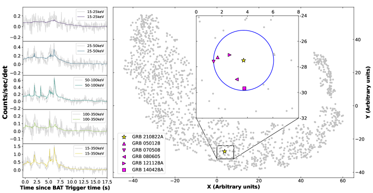
Figure 4: t-SNE visualization of the Swift//BAT data light curves using the method described by Garcia-Cifuentes et al. (2023b). The light curve obtained in the four bands of GRB 210822A by Swift/BAT in its automatic reduction pipeline is illustrated in the left panel. The blue circle indicates the equidistant region where the 5 closest events to GRB 210822A are located.

4.2.2 Optical

In the left panel of Figure 5, we compare the photometry of GRB 210822A in the $v$ filter obtained by the Swift/UVOT instrument (Siegel et al., 2021) with the current sample of remarkably bright long GRBs with Swift/UVOT light curves, presented by Oates (2023). This sample includes GRBs with unusual behaviour such as the ultra-bright GRB 061007, GRB 080319B, GRB 081203A, GRB 130427A, GRB 160625B, GRB 190114C, and GRB 221009A, all of which are classified as spectacular GRBs in terms of their brightness, when compared with other 56 UVOT-observed GRBs discovered between 2005 and 2010 (Oates et al., 2012).

We look at the $r$ band photometry for the same set of GRBs, presented in the left panel of Figure 5. We use the data from Mundell et al. (2007) (GRB 061007 , ), Bloom et al. (2009)(GRB 080319B), Rumyantsev et al. (2008); Volkov (2008); West et al. (2008) (GRB 081203A), Perley et al. (2014); Fraija et al. (2016) (GRB 130427A), Troja et al. (2017); Watson et al. (2016); Kuroda et al. (2016); Mazaeva et al. (2016a, b); Schweyer et al. (2016); Mazaeva et al. (2016c); Guidorzi et al. (2016); Valeev et al. (2016); Bikmaev et al. (2016) (GRB 160625B), Fraija et al. (2019) (GRB 190114C), Fulton et al. (2023); O’Connor et al. (2023) (GRB 221009A). We also plotted the optical light curves of standard GRBs from Becerra et al. (2023b) (gray solid lines) for comparison. For the estimation of the distances, we assume a $\Lambda$CDM model with a $H_{0}=67.8$ km/Mpc/s (Planck Collaboration et al., 2016).

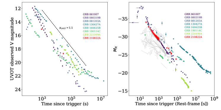
Figure 5: Comparison of optical light curves of GRB 210822A (red stars) and the brightest long GRBs presented by Oates (2023): GRB 061007 (thin diamonds, Mundell et al. (2007)), GRB 080319B (pentagons, Bloom et al. (2009)), GRB 081203A (up triangles, Rumyantsev et al. (2008); Volkov (2008); West et al. (2008)), GRB 130427A (filled circles, Perley et al. (2014); Fraija et al. (2016)), GRB 160625B (crosses, Troja et al. (2017); Watson et al. (2016); Kuroda et al. (2016); Mazaeva et al. (2016a, b); Guidorzi et al. (2016); Valeev et al. (2016); Bikmaev et al. (2016)), GRB 190114C (diamonds, Fraija et al. (2019)), and GRB 221009A (squares, Fulton et al. (2023); O’Connor et al. (2023)). Left: Optical light curves in the observer’s frame with the Swift/UVOT instrument in the V band. We plot a power-law segment that illustrates the typical decay of $\alpha_{\mathrm{UVOT}}=1.1$. Right: Optical light curves of the same set of GRBs and placed at their corresponding rest frame. We complement the sample with the GRBs with known redshift presented in Becerra et al. (2023b).

Table 4: Physical properties of the brightest Swift/UVOT long GRBs identified by Oates (2023) and the GRB 210822A. Information about duration and redshift is from the BAT catalogue. References: 1. Markwardt et al. (2006), 2. Fynbo et al. (2009), 3. Mundell et al. (2007), 4. Schady et al. (2008), 5. Panaitescu (2020), 6. Golenetskii et al. (2006), 7. Vreeswijk et al. (2008), 8. Racusin & Burrows (2009), 9. Tanvir et al. (2010), 10. Pandey et al. (2009), 11. Golenetskii et al. (2008), 12. Kuin et al. (2009), 13. Levan et al. (2013), 14. Perley et al. (2014), 15. Maselli et al. (2014), 16. Laskar et al. (2013), 17. Liu et al. (2013), 18. Golenetskii et al. (2013), 19. Burns (2016) 20. Xu et al. (2016), 21. Strausbaugh et al. (2019), 22. Lü2017, 23. Alexander et al. (2017), 24. Fraija et al. (2017), 25. Svinkin et al. (2016), 26. Selsing et al. (2019), 27. Misra et al. (2021), 28. Campana et al. (2021), 29. Frederiks et al. (2019), 30. Krimm et al. (2022), 31. Laskar et al. (2023), 32. An et al. (2023), 33. LHAASO Collaboration et al. (2023), 34. Negro et al. (2023), 35. Frederiks et al. (2023), 36. Lien et al. (2021), 37. Zhu et al. (2021), 38. Frederiks et al. (2021), 39. This work.

According to Figure 5, it can be seen that GRB 210822A has many similarities with the population of intrinsically bright GRBs (with $E_{\mathrm{iso}}\sim 10^{54}$ erg), sharing not only qualitative similarities in their temporal evolution, such as the observed slope and fluxes, but also their low redshift and opening angle $\theta_{\mathrm{j}}$ (see Table 4.2.2). Moreover, GRB 210822A shares the presence of a reverse shock component with GRB 080319B (Bloom et al., 2009), GRB 130427A (Perley et al., 2014), GRB 160625B (Zhang et al., 2018; Fraija et al., 2017), GRB 190114C (Laskar et al., 2019; Fraija et al., 2019) and GRB 221009A (Laskar et al., 2023; Zhang et al., 2023; Bright et al., 2023; Gill & Granot, 2023).

It is important to note that none of these events share a significant gamma-ray brightness, as discussed in detail in Section 4.2.1. This suggests that the optical emission and the gamma ray emission have different origins. Moreover, this illustrates the need to make multi-frequency observations for a complete understanding of each GRB.

The information provided in Table 4.2.2 suggests that GRB 210822A and the extremely bright optical LGRBs considered in this work, share an intrinsically high isotropic energy ($E_{\mathrm{iso}}$) and luminosity ($L_{\mathrm{iso}}$). This, combined with the similarity found in their optical photometry, leads us to assume i) more extreme central engine properties which are thought to originate from a binary-driven hypernova produced by a binary system composed of a carbon-oxygen star and a neutron star unlike the conventional GRBs (Rueda et al., 2020) or, ii) a specific configuration for the observer of a structured jet (Lan et al., 2023).

That said, Lan et al. (2023) compared the host galaxies of these intense GRBs with more conventional LGRBs and examined the energy, and they revealed no significant differentiation between these event groups.

The most accepted scenarios discussed for progenitors of LGRBs are a rapidly accreting black hole (BH, Narayan et al., 1992; Woosley, 1993; Fryer et al., 1999) and a rapidly spinning, strongly magnetised neutron star (NS) (a millisecond magnetar; Duncan & Thompson, 1992; Usov, 1992; Thompson, 1994). In the first scenario, the collapse of massive stars typically leads to a BH plus a long-lived debris torus system (e.g., see Woosley, 1993). The relativistic jet is powered by extraction mediated by accretion from a Kerr BH (Blandford & Znajek, 1977). When the star collapses into a BH, the stellar core must retain enough angular momentum to spin fast enough to generate an accretion disk. In the last scenario, a millisecond magnetar is generated with a large rotational energy to impede the gravitational collapse (e.g., see Metzger et al., 2011). The relativistic outflow is powered by the spin-down luminosity of the magnetic dipole, and the maximum energy reservoir becomes $\approx 2\times 10^{52}\,{\rm erg}\,M_{\rm ns}^{\frac{3}{2}}P^{-2}_{-3}$ with $M_{\rm ns}$ the mass of the NS and $P$ the corresponding spin period. Multiwavelength afterglow observations during the early phases provide valuable insights into elucidating the characteristics of the progenitors, the mass-loss evolution, metallicity, and establishing limits on the density of the surrounding medium (Ackermann et al., 2013; Fraija et al., 2019; Fraija et al., 2020). For instance, metallicity plays a relevant role in wind mass loss, along with rotation, determining the final phase angular momentum and, therefore, the destiny of the massive star. A millisecond magnetar can hardly explain a burst with isotropic energy larger than $10^{53}\,{\rm erg}$ and disfavor bursts that exhibit an optical flare due to a large magnetisation that would suppress the reverse shock (e.g., see Zhang & Kobayashi, 2005). Otherwise, highly bright LGRBs favour massive star progenitors with low metallicity (Perley et al., 2014; Zhang et al., 2018).

5 Conclusions

We have presented optical photometry of the afterglow of the ultra-bright GRB 210822A, combining new data from the RATIR instrument from $T+0.02$ to $T+0.49$ hours after the Swift trigger and with photometry from other telescopes published in GCN/TAN alerts.

We have compared the optical light curve and the X-ray obtained from Swift/XRT and Swift/UVOT, respectively. The photometric data reveal an achromatic temporal evolution well modelled by the expected evolution of an afterglow. The spectral indices measured at $T+500$ and $T+43000$ suggest the spectral regime where $\nu_{\mathrm{m}}<\nu_{\mathrm{opt}}<\nu_{X}<\nu_{c}$ corresponds to a flux evolving as $F\propto\nu^{\frac{p-1}{2}}t^{\frac{3(1-p)}{4}}$ with $p=2.54\pm 0.10$.

Furthermore, we identified a reverse shock component in the optical bands before $T+300$ s. We also see a change in slope between $T+80000$ s and $T+100000$ s that we interpret as the signature of a jet break, allowing us to estimate a jet opening angle of about $\theta_{\mathrm{j}}=3-5^{\circ}$.

We use machine-learning techniques to model the light curves and constrain the intrinsic parameters of the burst. The technique used in this work is able to learn directly from the data and correct the model to use for fitting. This approach mitigates the challenges associated with conventional spline or polynomial interpolation methods and avoids excessive overfitting treatments.

In a general context, we showed the similarity of GRB 210822A with other events that are extremely bright in the optical/UV such as GRB 080319B, GRB 160625A GRB 190114C, GRB 221009A and GRB 130427A, which allows us to place GRB210822A in a peculiar group of GRBs with remarkably bright afterglows. Nevertheless, this set of GRBs differs from the events that share features in gamma-rays, evidencing the different regions and emission processes in which each of these frequencies originate.

Finally, we underscore the importance of early-to-late ground-based telescope observations following a trigger, coupled with the essential supplementation of optical photometry data from Swift/XRT and Swift/UVOT. This combined approach is indispensable to achieve a comprehensive understanding of the GRB phenomena. Using earlier observations, we were able to model the reverse shock component and determine the level of low magnetisation present in this GRB. On the other hand, later observations constrain the opening angle and, therefore, the geometry of the jet, providing us with clues about the type of progenitor that produced GRB 210822A.

Acknowledgements

The authors would like to thank the anonymous reviewer for his/her valuable comments. Some of the data used in this paper were acquired with the RATIR instrument, funded by the University of California and NASA Goddard Space Flight Center, and the 1.5-meter Harold L. Johnson telescope at the Observatorio Astronómico Nacional on the Sierra de San Pedro Mártir, operated and maintained by the Observatorio Astronómico Nacional and the Instituto de Astronomía of the Universidad Nacional Autónoma de México. Operations are partially funded by the Universidad Nacional Autónoma de México (DGAPA/PAPIIT IG100414, IT102715, AG100317, IN109418, IG100820, IN106521 and IN105921). FDC acknowledges the computing time granted by DGTIC UNAM on the supercomputer Miztli (project LANCAD-UNAM-DGTIC-281). We acknowledge the contribution of Leonid Georgiev and Neil Gehrels to the development of RATIR.

The authors thank the staff of the Observatorio Astronómico Nacional.

We acknowledge the support from the DGAPA/PAPIIT grants IG100422 and IN113424.

This work made use of data supplied by the UK Swift Science Data Centre at the University of Leicester.

CAV, KGC, and FV acknowledge support from CONAHCyT fellowship. RLB acknowledges support from the CONAHCyT postdoctoral fellowship.

Research Data Policy

The data underlying this article will be shared on reasonable request to the corresponding author. The Swift/BAT and Swift/XRT data presented in this work are public and can be found in the domain https://www.swift.ac.uk/xrt$_$products/index.php.

Appendix A Neural Network Implementation

In this study, we presented a machine learning approach that harnesses the power of 30,000 synthetic GRBs models to automatically generate models from observational data. While the generation of these synthetic datasets may be time-intensive, the training of our machine learning model is remarkably efficient. Furthermore, the application of the model to new observational data is even faster. A noteworthy advantage of this methodology is its versatility, as the trained ML model can be applied to a wide range of observational data, provided that the GRB models in question fall within the parameter space covered by the 30,000 synthetic models. This approach offers a powerful and expedient tool for modeling and analyzing GRBs, with the potential to significantly accelerate research in this field.

The implemented neural network architecture consists of a deep feedforward neural network with distinct layers. It incorporates multiple hidden layers and follows a pattern of stacking fully connected (dense) layers with activation functions, including ReLU and linear. Dropout layers are incorporated at various points within the architecture, serving as a form of regularisation to mitigate the risk of overfitting.

The final layer produces the output of the network output, producing predictions based on the initial input. This architecture allows the network to learn and model complex relationships within the data, contributing to its predictive capabilities. The idea is that we train the code with synthetic light curves as inputs and the eight parameters as outputs, so we can use the trained model to find parameters based on observed light curves.

Parameter	Range
$\theta_{\mathrm{obs}}$	$0.001$ to $0.150$ rad
$E$	$10^{53}$ to $10^{55}$ erg
$\theta_{\mathrm{j}}$	$0.001$ to $0.100$ rad
$p$	$2.01$ to $3.00$
$\epsilon_{\mathrm{e}}$	$10^{-7}$ to $10^{-1}$
$\epsilon_{\mathrm{B}}$	$10^{-7}$ to $10^{-1}$
$\chi$	$0.8$ to $1.0$
$n_{\mathrm{0}}$	$0.7$ to $1.0$ cm-3

Table 5: Interval of each parameter used in the synthetic data generation.

The ML model was trained over a span of 14 epochs (Figure 6). The number of training epochs is automatically determined through the implementation of an early stopping mechanism, the EarlyStopping function . This mechanism monitors the training process and stops training when convergence is detected in the loss function, facilitating efficient training by preventing overfitting and unnecessary iterations. The dataset was partitioned into three distinct sets: the training data, consisting of 25000 synthetic data points; the validation data, comprising 3000 samples; and the test data, with a total of 2000 samples. During each epoch, the ML model attempted to validate its learning by comparing its predictions against the validation dataset, which is not used in the training process. The primary objective of the training process is to minimise the loss function, the Mean Squared Error (MSE).

Once the model is adequately trained, it is evaluated against the test data set, which is used to estimate the errors in the parameters and to verify the absence of overfitting, which would restrict the neural network to reproducing only the training and validation data. Figure 6 presents the temporal evolution of the loss function for both training and validation data.

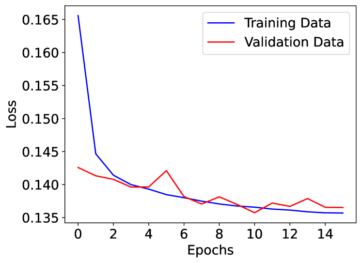
Figure 6: Temporal evolution of the loss function for training (blue) and validation data (red)

References

- Ackermann et al. (2013) Ackermann M., et al., 2013, ApJ, 763, 71
- Ahumada et al. (2021) Ahumada T., et al., 2021, Nature Astronomy, 5, 917
- Alexander et al. (2017) Alexander K. D., et al., 2017, ApJ, 848, 69
- An et al. (2023) An Z.-H., et al., 2023, arXiv e-prints, p. arXiv:2303.01203
- Arnaud (1996) Arnaud K. A., 1996, in Jacoby G. H., Barnes J., eds, Astronomical Society of the Pacific Conference Series Vol. 101, Astronomical Data Analysis Software and Systems V. p. 17
- Barthelmy et al. (2007) Barthelmy S. D., et al., 2007, GRB Coordinates Network, 6390, 1
- Becerra et al. (2017) Becerra R. L., et al., 2017, ApJ, 837, 116
- Becerra et al. (2019a) Becerra R. L., et al., 2019a, ApJ, 881, 12
- Becerra et al. (2019b) Becerra R. L., et al., 2019b, ApJ, 887, 254
- Becerra et al. (2023a) Becerra R. L., et al., 2023a, MNRAS, 522, 5204
- Becerra et al. (2023b) Becerra R. L., et al., 2023b, MNRAS, 525, 3262
- Belkin et al. (2021a) Belkin S., Kusakin A., Reva I., Pozanenko Pankov N., Kim V., GRB-IKI-FuN 2021a, GRB Coordinates Network, 30712, 1
- Belkin et al. (2021b) Belkin S., Kusakin A., Reva I., Pozanenko Pankov N., Kim V., GRB-IKI-FuN 2021b, GRB Coordinates Network, 30714, 1
- Berger (2014) Berger E., 2014, ARA&A, 52, 43
- Bertin & Arnouts (1996) Bertin E., Arnouts S., 1996, A&AS, 117, 393
- Bikmaev et al. (2016) Bikmaev I., et al., 2016, GRB Coordinates Network, 19651, 1
- Blandford & Znajek (1977) Blandford R. D., Znajek R. L., 1977, MNRAS, 179, 433
- Bloom et al. (2009) Bloom J. S., et al., 2009, ApJ, 691, 723
- Bright et al. (2023) Bright J. S., et al., 2023, Nature Astronomy, 7, 986
- Burns (2016) Burns E., 2016, GRB Coordinates Network, 19587, 1
- Butler et al. (2012) Butler N., et al., 2012, in McLean I. S., Ramsay S. K., Takami H., eds, Society of Photo-Optical Instrumentation Engineers (SPIE) Conference Series Vol. 8446, Ground-based and Airborne Instrumentation for Astronomy IV. p. 844610, doi:10.1117/12.926471
- Butler et al. (2021) Butler N., et al., 2021, GRB Coordinates Network, 30680, 1
- Campana et al. (2021) Campana S., Lazzati D., Perna R., Grazia Bernardini M., Nava L., 2021, A&A, 649, A135
- Chollet (2015) Chollet F. e. a., 2015, Keras, https://keras.io
- Duncan & Thompson (1992) Duncan R. C., Thompson C., 1992, ApJ, 392, L9
- Evans et al. (2007) Evans P. A., et al., 2007, A&A, 469, 379
- Evans et al. (2009) Evans P. A., et al., 2009, MNRAS, 397, 1177
- Ferreira et al. (2020) Ferreira L., Conselice C. J., Duncan K., Cheng T.-Y., Griffiths A., Whitney A., 2020, ApJ, 895, 115
- Fraija et al. (2016) Fraija N., Lee W., Veres P., 2016, ApJ, 818, 190
- Fraija et al. (2017) Fraija N., et al., 2017, ApJ, 848, 15
- Fraija et al. (2019) Fraija N., Dichiara S., Pedreira A. C. C. d. E. S., Galvan-Gamez A., Becerra R. L., Barniol Duran R., Zhang B. B., 2019, ApJ, 879, L26
- Fraija et al. (2020) Fraija N., Laskar T., Dichiara S., Beniamini P., Duran R. B., Dainotti M. G., Becerra R. L., 2020, ApJ, 905, 112
- Frederiks et al. (2019) Frederiks D., et al., 2019, GRB Coordinates Network, 23737, 1
- Frederiks et al. (2021) Frederiks D., et al., 2021, GRB Coordinates Network, 30694, 1
- Frederiks et al. (2023) Frederiks D., et al., 2023, ApJ, 949, L7
- Fryer et al. (1999) Fryer C. L., Woosley S. E., Hartmann D. H., 1999, ApJ, 526, 152
- Fu et al. (2021) Fu S. Y., Zhu Z. P., Liu X., Xu D., Gao X., Liu J. Z., 2021, GRB Coordinates Network, 30684, 1
- Fulton et al. (2023) Fulton M. D., et al., 2023, ApJ, 946, L22
- Fynbo et al. (2009) Fynbo J. P. U., et al., 2009, ApJS, 185, 526
- Gao & Mészáros (2015) Gao H., Mészáros P., 2015, Advances in Astronomy, 2015, 192383
- Garcia-Cifuentes et al. (2023a) Garcia-Cifuentes K., Becerra R. L., De Colle F., Vargas F., 2023a, arXiv e-prints, p. arXiv:2309.15825
- Garcia-Cifuentes et al. (2023b) Garcia-Cifuentes K., Becerra R. L., De Colle F., Cabrera J. I., Del Burgo C., 2023b, ApJ, 951, 4
- García-García et al. (2023) García-García L., López-Cámara D., Lazzati D., 2023, MNRAS, 519, 4454
- Gill & Granot (2023) Gill R., Granot J., 2023, MNRAS, 524, L78
- Gill et al. (2019) Gill R., Granot J., De Colle F., Urrutia G., 2019, ApJ, 883, 15
- Golenetskii et al. (2006) Golenetskii S., Aptekar R., Mazets E., Pal’Shin V., Frederiks D., Cline T., 2006, GRB Coordinates Network, 5722, 1
- Golenetskii et al. (2008) Golenetskii S., Aptekar R., Mazets E., Pal’Shin V., Frederiks D., Cline T., 2008, GRB Coordinates Network, 7482, 1
- Golenetskii et al. (2013) Golenetskii S., et al., 2013, GRB Coordinates Network, 14487, 1
- Gomboc et al. (2009) Gomboc A., et al., 2009, in Meegan C., Kouveliotou C., Gehrels N., eds, American Institute of Physics Conference Series Vol. 1133, Gamma-ray Burst: Sixth Huntsville Symposium. pp 145–150 (arXiv:0902.1830), doi:10.1063/1.3155867
- Gordon et al. (2003) Gordon K. D., Clayton G. C., Misselt K. A., Landolt A. U., Wolff M. J., 2003, ApJ, 594, 279
- Granot (2012) Granot J., 2012, MNRAS, 421, 2610
- Granot & Sari (2002) Granot J., Sari R., 2002, ApJ, 568, 820
- Guidorzi et al. (2016) Guidorzi C., Kobayashi S., Mundell C. G., Gomboc A., 2016, GRB Coordinates Network, 19640, 1
- Hjorth et al. (2003) Hjorth J., et al., 2003, Nature, 423, 847
- Jakobsson et al. (2007) Jakobsson P., et al., 2007, GRB Coordinates Network, 6398, 1
- Jespersen et al. (2020) Jespersen C. K., Severin J. B., Steinhardt C. L., Vinther J., Fynbo J. P. U., Selsing J., Watson D., 2020, ApJ, 896, L20
- Kann et al. (2021) Kann D. A., de Ugarte Postigo A., Thoene C., Blazek M., Agui Fernandez J. F., Fernandez A., Hermelo I., Martin P., 2021, GRB Coordinates Network, 30723, 1
- Kouveliotou et al. (1993) Kouveliotou C., Meegan C. A., Fishman G. J., Bhat N. P., Briggs M. S., Koshut T. M., Paciesas W. S., Pendleton G. N., 1993, ApJ, 413, L101
- Krimm et al. (2014) Krimm H. A., et al., 2014, GRB Coordinates Network, 16186, 1
- Krimm et al. (2022) Krimm H. A., et al., 2022, GRB Coordinates Network, 32688, 1
- Kuin et al. (2009) Kuin N. P. M., et al., 2009, MNRAS, 395, L21
- Kumar & Zhang (2015) Kumar P., Zhang B., 2015, Phys. Rep., 561, 1
- Kuroda et al. (2016) Kuroda D., et al., 2016, GRB Coordinates Network, 19599, 1
- LHAASO Collaboration et al. (2023) LHAASO Collaboration et al., 2023, Science, 380, 1390
- Lan et al. (2023) Lan L., et al., 2023, ApJ, 949, L4
- Lang et al. (2010) Lang D., Hogg D. W., Mierle K., Blanton M., Roweis S., 2010, AJ, 139, 1782
- Laskar et al. (2013) Laskar T., et al., 2013, ApJ, 776, 119
- Laskar et al. (2019) Laskar T., et al., 2019, ApJ, 878, L26
- Laskar et al. (2023) Laskar T., et al., 2023, ApJ, 946, L23
- Lee & Ramirez-Ruiz (2007) Lee W. H., Ramirez-Ruiz E., 2007, New Journal of Physics, 9, 17
- Levan et al. (2013) Levan A. J., Cenko S. B., Perley D. A., Tanvir N. R., 2013, GRB Coordinates Network, 14455, 1
- Levan et al. (2023) Levan A., et al., 2023, arXiv e-prints, p. arXiv:2307.02098
- Li et al. (2012) Li L., et al., 2012, ApJ, 758, 27
- Liang et al. (2010) Liang E.-W., Yi S.-X., Zhang J., Lü H.-J., Zhang B.-B., Zhang B., 2010, ApJ, 725, 2209
- Lien et al. (2021) Lien A. Y., et al., 2021, GRB Coordinates Network, 30689, 1
- Littlejohns et al. (2015) Littlejohns O. M., et al., 2015, MNRAS, 449, 2919
- Liu et al. (2013) Liu R.-Y., Wang X.-Y., Wu X.-F., 2013, ApJ, 773, L20
- Lochner et al. (2016) Lochner M., McEwen J. D., Peiris H. V., Lahav O., Winter M. K., 2016, ApJS, 225, 31
- MacFadyen & Woosley (1999) MacFadyen A. I., Woosley S. E., 1999, ApJ, 524, 262
- Malik et al. (2021) Malik A., Moster B. P., Obermeier C., 2021, Monthly Notices of the Royal Astronomical Society, 513, 5505
- Markwardt et al. (2006) Markwardt C., et al., 2006, GRB Coordinates Network, 5713, 1
- Maselli et al. (2014) Maselli A., et al., 2014, Science, 343, 48
- Mazaeva et al. (2016a) Mazaeva E., Kusakin A., Minaev P., Reva I., Volnova A., Pozanenko A., 2016a, GRB Coordinates Network, 19605, 1
- Mazaeva et al. (2016b) Mazaeva E., Kusakin A., Minaev P., Reva I., Volnova A., Pozanenko A., 2016b, GRB Coordinates Network, 19619, 1
- Mazaeva et al. (2016c) Mazaeva E., Kusakin A., Minaev P., Reva I., Volnova A., Pozanenko A., 2016c, GRB Coordinates Network, 19680, 1
- Mészáros & Rees (1997) Mészáros P., Rees M. J., 1997, ApJ, 476, 232
- Mészáros & Rees (1999) Mészáros P., Rees M. J., 1999, MNRAS, 306, L39
- Metzger et al. (2011) Metzger B. D., Giannios D., Thompson T. A., Bucciantini N., Quataert E., 2011, MNRAS, 413, 2031
- Misra et al. (2021) Misra K., et al., 2021, MNRAS, 504, 5685
- Monet et al. (2003) Monet D. G., et al., 2003, AJ, 125, 984
- Mundell et al. (2007) Mundell C. G., et al., 2007, ApJ, 660, 489
- Narayan et al. (1992) Narayan R., Paczynski B., Piran T., 1992, ApJ, 395, L83
- Negro et al. (2023) Negro M., et al., 2023, ApJ, 946, L21
- Ni (2016) Ni W.-T., 2016, International Journal of Modern Physics D, 25, 1630001
- Nicuesa Guelbenzu et al. (2021) Nicuesa Guelbenzu A., Klose S., Rau A., 2021, GRB Coordinates Network, 30703, 1
- O’Connor et al. (2023) O’Connor B., et al., 2023, Science Advances, 9, eadi1405
- Oates (2023) Oates S., 2023, Universe, 9, 113
- Oates et al. (2009) Oates S. R., et al., 2009, MNRAS, 395, 490
- Oates et al. (2012) Oates S. R., Page M. J., De Pasquale M., Schady P., Breeveld A. A., Holland S. T., Kuin N. P. M., Marshall F. E., 2012, MNRAS, 426, L86
- Page et al. (2021) Page K. L., Gropp J. D., Kuin N. P. M., Lien A. Y., Neil Gehrels Swift Observatory Team 2021, GRB Coordinates Network, 30677, 1
- Palmer et al. (2012) Palmer D. M., et al., 2012, GRB Coordinates Network, 14011, 1
- Panaitescu (2020) Panaitescu A., 2020, ApJ, 895, 39
- Pandey et al. (2009) Pandey S. B., et al., 2009, A&A, 504, 45
- Pereyra et al. (2022) Pereyra M., et al., 2022, MNRAS, 511, 6205
- Perley (2014) Perley D. A., 2014, GRB Coordinates Network, 16181, 1
- Perley et al. (2014) Perley D. A., et al., 2014, ApJ, 781, 37
- Perri et al. (2021) Perri M., et al., 2021, GRB Coordinates Network, 30691, 1
- Planck Collaboration et al. (2016) Planck Collaboration et al., 2016, A&A, 594, A13
- Racusin & Burrows (2009) Racusin J. L., Burrows D. N., 2009, AIP Conference Proceedings, 1133, 157
- Rastinejad et al. (2022) Rastinejad J. C., et al., 2022, Nature, 612, 223
- Romanov & Lane (2021) Romanov F. D., Lane D. J., 2021, GRB Coordinates Network, 30701, 1
- Rueda et al. (2020) Rueda J. A., Ruffini R., Karlica M., Moradi R., Wang Y., 2020, ApJ, 893, 148
- Rumyantsev et al. (2008) Rumyantsev V., Antonyuk K., Andreev M., Pozanenko A., 2008, GRB Coordinates Network, 8645, 1
- Ryan et al. (2020) Ryan G., van Eerten H., Piro L., Troja E., 2020, ApJ, 896, 166
- Sanchez-Alarcon & Ascasibar Sequeiros (2022) Sanchez-Alarcon P. M., Ascasibar Sequeiros Y., 2022, arXiv e-prints, p. arXiv:2201.05145
- Sari & Piran (1997) Sari R., Piran T., 1997, ApJ, 485, 270
- Sari & Piran (1999) Sari R., Piran T., 1999, ApJ, 520, 641
- Sari et al. (1998) Sari R., Piran T., Narayan R., 1998, ApJ, 497, L17
- Schady et al. (2008) Schady P., et al., 2008, in Galassi M., Palmer D., Fenimore E., eds, American Institute of Physics Conference Series Vol. 1000, Gamma-ray Bursts 2007. pp 200–203 (arXiv:astro-ph/0611081), doi:10.1063/1.2943443
- Schlegel et al. (1998) Schlegel D. J., Finkbeiner D. P., Davis M., 1998, ApJ, 500, 525
- Schweyer et al. (2016) Schweyer T., Chen T. W., Greiner J., 2016, GRB Coordinates Network, 19629, 1
- Selsing et al. (2019) Selsing J., Fynbo J. P. U., Heintz K. E., Watson D., 2019, GRB Coordinates Network, 23695, 1
- Siegel et al. (2021) Siegel M. H., Page K. L., Swift/UVOT Team 2021, GRB Coordinates Network, 30710, 1
- Skrutskie et al. (2006) Skrutskie M. F., et al., 2006, AJ, 131, 1163
- Steinhardt et al. (2023) Steinhardt C. L., Mann W. J., Rusakov V., Jespersen C. K., 2023, ApJ, 945, 67
- Strausbaugh et al. (2019) Strausbaugh R., Butler N., Lee W. H., Troja E., Watson A. M., 2019, ApJ, 873, L6
- Svinkin et al. (2016) Svinkin D., et al., 2016, GRB Coordinates Network, 19604, 1
- Tanvir et al. (2010) Tanvir N. R., et al., 2010, ApJ, 725, 625
- Tanvir et al. (2012) Tanvir N. R., Levan A. J., Matulonis T., 2012, GRB Coordinates Network, 14009, 1
- Thompson (1994) Thompson C., 1994, MNRAS, 270, 480
- Troja et al. (2017) Troja E., et al., 2017, Nature, 547, 425
- Troja et al. (2022) Troja E., et al., 2022, Nature, 612, 228
- Usov (1992) Usov V. V., 1992, Nature, 357, 472
- Valeev et al. (2016) Valeev A. F., Moskvitin A. S., Beskin G. M., Vlasyuk V. V., Sokolov V. V., 2016, GRB Coordinates Network, 19642, 1
- Vogl et al. (2020) Vogl C., Kerzendorf W. E., Sim S. A., Noebauer U. M., Lietzau S., Hillebrandt W., 2020, AAP, 633, A88
- Volkov (2008) Volkov I., 2008, GRB Coordinates Network, 8604, 1
- Vreeswijk et al. (2008) Vreeswijk P. M., Smette A., Malesani D., Fynbo J. P. U., Milvang-Jensen B., Jakobsson P., Jaunsen A. O., Ledoux C., 2008, GRB Coordinates Network, 7444, 1
- Wang et al. (2018) Wang X.-G., Zhang B., Liang E.-W., Lu R.-J., Lin D.-B., Li J., Li L., 2018, ApJ, 859, 160
- Watson et al. (2012) Watson A. M., et al., 2012, in Stepp L. M., Gilmozzi R., Hall H. J., eds, Society of Photo-Optical Instrumentation Engineers (SPIE) Conference Series Vol. 8444, Ground-based and Airborne Telescopes IV. p. 84445L, doi:10.1117/12.926927
- Watson et al. (2016) Watson A. M., et al., 2016, GRB Coordinates Network, 19602, 1
- West et al. (2008) West J. P., et al., 2008, GRB Coordinates Network, 8617, 1
- Woosley (1993) Woosley S. E., 1993, ApJ, 405, 273
- Xiao & Schaefer (2011) Xiao L., Schaefer B. E., 2011, ApJ, 731, 103
- Xu et al. (2016) Xu D., Malesani D., Fynbo J. P. U., Tanvir N. R., Levan A. J., Perley D. A., 2016, GRB Coordinates Network, 19600, 1
- Yang et al. (2023) Yang Y.-H., et al., 2023, arXiv e-prints, p. arXiv:2308.00638
- Zhang & Kobayashi (2005) Zhang B., Kobayashi S., 2005, ApJ, 628, 315
- Zhang & Yan (2011) Zhang B., Yan H., 2011, ApJ, 726, 90
- Zhang et al. (2006) Zhang B., Fan Y. Z., Dyks J., Kobayashi S., Mészáros P., Burrows D. N., Nousek J. A., Gehrels N., 2006, ApJ, 642, 354
- Zhang et al. (2018) Zhang B. B., et al., 2018, Nature Astronomy, 2, 69
- Zhang et al. (2021) Zhang B. B., et al., 2021, Nature Astronomy, 5, 911
- Zhang et al. (2023) Zhang B. T., Murase K., Ioka K., Song D., Yuan C., Mészáros P., 2023, ApJ, 947, L14
- Zheng et al. (2021) Zheng W., Filippenko A. V., KAIT GRB Team 2021, GRB Coordinates Network, 30679, 1
- Zhu et al. (2021) Zhu Z. P., Izzo L., Fu S. Y., Xu D., Fynbo J. P. U., Paraskeva E., Vitali S., 2021, GRB Coordinates Network, 30692, 1
- van Eerten & MacFadyen (2012) van Eerten H. J., MacFadyen A. I., 2012, ApJ, 747, L30
- van der Maaten & Hinton (2008) van der Maaten L., Hinton G., 2008, Journal of Machine Learning Research, 9, 2579