A Semi-Supervised Approach for Power System Event Identification

Abstract

Event identification is increasingly recognized as crucial for enhancing the reliability, security, and stability of the electric power system. With the growing deployment of Phasor Measurement Units (PMUs) and advancements in data science, there are promising opportunities to explore data-driven event identification via machine learning classification techniques. However, obtaining accurately-labeled eventful PMU data samples remains challenging due to its labor-intensive nature and uncertainty about the event type (class) in real-time. Thus, it is natural to use semi-supervised learning techniques, which make use of both labeled and unlabeled samples. We evaluate three categories of classical semi-supervised approaches: (i) self-training, (ii) transductive support vector machines (TSVM), and (iii) graph-based label spreading (LS) method. Our approach characterizes events using physically interpretable features extracted from modal analysis of synthetic eventful PMU data. In particular, we focus on the identification of four event classes (load loss, generation loss, line trip, and bus fault) whose identification is crucial for grid operations. We have developed and publicly shared a comprehensive Event Identification package which consists of three aspects: data generation, feature extraction, and event identification with limited labels using semi-supervised methodologies. Using this package, we generate and evaluate eventful PMU data for the South Carolina 500-Bus synthetic network. Our evaluation consistently demonstrates that graph-based LS outperforms the other two semi-supervised methods that we consider, and can noticeably improve event identification performance relative to the setting with only a small number of labeled samples.

I Introduction

Power systems are inherently complex dynamical systems, primarily due to the involvement of diverse components such as generators, buses, lines, and loads with varying sizes, all exhibiting non-linear behavior and intricate interactions. Given their extensive geographical coverage and scale, power systems are susceptible to various classes of events (for example, generation loss, load loss, line trips). Event identification methods can be used in real-time operations to guide control actions, as well as for off-line analysis of past events to make the system more reliable, secure, and stable in the future. Numerous studies have explored event detection in power systems, focusing on determining whether an event has occurred [1, 2, 3]. However, event identification, which involves discerning the specific class of event that occurred, presents even greater challenges since it requires learning the unique signatures of different events. Our primary focus here is on addressing the event identification problem in power systems. To this end, our analysis in the sequel assumes that an event has been detected with knowledge of its precise time.

The increasing deployment of Phasor Measurement Units (PMUs) throughout the grid, coupled with advancements in machine learning techniques, presents invaluable opportunities for exploring advanced data-driven event identification methods. These methods offer the distinct advantage of differentiating between various classes of power system events based on high-dimensional spatio-temporally correlated time-synchronized phasor measurements with high resolution, without heavily relying on dynamic modeling of power system components. The majority of the recent literature in the field of data-driven event identification (e.g., [4, 5, 6, 7, 8, 9, 10, 11, 12]) employs machine learning and pattern recognition techniques for making statistical inferences or decisions using system measurements. A significant portion of these studies predominantly falls within the supervised learning paradigm, which requires accurate labeled data. However, acquiring expert knowledge for labeling various classes of events can be expensive and laborious. Consequently, the manual labeling of events by operators constitutes only about 2% of the events [13]. Such limitations motivate researchers to leverage simulation-based synthetic eventful PMU data for investigating and evaluating the performance of their proposed event identification methods (e.g., [14, 15, 8]). Despite the availability of several resources providing access to synthetic test cases with transmission and/or distribution network models for dynamic simulations [16, 17], conducting a fair comparison of diverse event identification methods might pose a significant challenge. This challenge primarily stems from the numerous parameters associated with dynamic models of system components and simulation settings, coupled with the diverse characteristics of simulated events, such as class, duration, and location, among others. While certain recent publications may have access to significant real and/or synthetic PMU data (e.g., [18, 19]), the lack of publicly available properly labeled eventful PMU data continues to be a persistent concern for numerous researchers.

Unsupervised and semi-supervised learning are common practices in machine learning when dealing with no or limited labeled data. Unsupervised learning aims to infer the underlying structure within the unlabeled data. Although they can distinguish between clusters of events [2, 20, 21, 22, 23, 24], they do not possess the ground truth to associate each cluster with its real-world meaning. Furthermore, when there is access to even a small amount of labeled data, supervised learning has been shown to perform better than unsupervised learning methods [2, 24]. Semi-supervised learning approaches, on the other hand, aim to label unlabeled data points using knowledge learned from a small number of labeled data points which can significantly enhance the performance of a classification task [25]. Reference [18] presents a framework for event detection, localization, and classification in power grids based on semi-supervised learning. A pseudo labeling (PL) technique is adopted to classify events using the convolutional neural network (CNN) backbone with cross-entropy loss. A semi-supervised event identification framework is proposed in [26] which utilizes a hybrid machine learning-based method to reduce biases of different classifiers. In [27], the authors explore the application of deep learning techniques and PMU data to develop real-time event identification models for transmission networks. This is achieved by leveraging information from a large pool of unlabeled events, while also taking into account the class distribution mismatch problem. In [28, 29], the authors proposed hidden structure semi-supervised machine (HS3M), a novel data-driven event identification method that combines unlabeled and partially labeled data to address limitations in supervised, semi-supervised, and hidden structure learning. The approach introduces a parametric dual optimization procedure to enhance the learning objective and improve event identification accuracy. The learning problem involves optimizing a non-smooth function that may be convex or concave.

The existing literature on neural network-based event identification methods is marked by certain limitations and challenges. These encompass the scarcity of suitable historical labeled event data, restricted interpretability in feature extraction, elevated computational intricacy, and the necessity for meticulous parameter calibration. Additionally, pseudo labeling approaches such as [28] confront uncertainty regarding the attainability of global optimality. Moreover, it is worth noting that, to the best of the authors’ knowledge, a thorough investigation into the ramifications arising from the initial distribution of labeled and unlabeled samples has not been undertaken. Building upon the promising results of our previous work on event identification in the supervised setting [30], this paper introduces a semi-supervised event identification framework. The aim of this study is to explore the potential benefits of incorporating unlabeled samples in enhancing the performance of the event identification task. To this end, we thoroughly investigate and compare the performance of various semi-supervised algorithms, including: (i) self-training with different base classifiers (i.e., support vector machine with linear kernel (SVML) as well as with radial basis function kernel (SVMR), gradient boosting (GB), decision trees (DT), and k-Nearest Neighbors (kNN)), (ii) transductive support vector machines (TSVM), and (iii) graph-based label spreading (LS) to explore their effectiveness. We chose these classical semi-supervised models for two primary reasons: firstly, the wide array of proposed semi-supervised classification algorithms in the past two decades (see, [31], and references therein) necessitates a comprehensive understanding of which models are most suitable and efficient for event identification; and secondly, they provide a clearer illustration and intuition of the impact of incorporating unlabeled samples compared to more advanced methods. Although there may not be a one-size-fits-all solution, each method has its own advantages and disadvantages, and it is important to evaluate their suitability. Notably, our experiments consistently illustrate the superior performance of the graph-based LS method compared to other approaches. Even in worst-case scenarios where the initial distribution of labeled and unlabeled samples does not necessarily reflect the true distribution of event classes, the graph-based LS method stands out in robustly and significantly enhancing event identification performance. Our key contributions are as follows:

• Introduction of a semi-supervised event identification framework that leverages physically interpretable features derived from modal analysis of PMU data.

• Thorough exploration of the influence of the initial distribution of labeled and unlabeled samples, along with the quantity of unlabeled samples, on the efficacy of diverse semi-supervised event identification techniques.

• Development of an all-inclusive Event Identification package comprising of an event generation module based on the power system simulator for engineering (PSS^®E) Python application programming interface (API), a feature extraction module utilizing methodologies from our previous research [30], and a semi-supervised classification module.

The remainder of the paper is organized as follows. Section. II describes the simulation process to generate the synthetic eventful PMU data. We explain the proposed semi-supervised event identification framework in Section. III. In Section. IV, we further elaborate on the pseudo labeling process of the unlabeled samples, and the classification models. We discuss the simulation results in Section. V. Finally, Section. VI concludes the paper.

II Generation of the Synthetic Eventful Time-series PMU Data

Consider an electric grid composed of set of loads, generators, lines, and buses. We investigate four distinct event classes denoted as $\mathcal{E}\in\{\text{LL, GL, LT, BF}\}$, representing load loss, generation loss, line trip, and bus fault events, respectively. Each PMU provides multiple measurement channels relative to its installation bus. In this study, we focus on voltage magnitude ($V_{m}$), corresponding angle ($V_{a}$), and frequency ($F$) channels for clarity, with potential inclusion of other channels. For any channel $c\in\mathcal{C}=\{V_{m},V_{a},F\}$, let $y^{c}_{i}(n)\in\mathbb{R}$ represent the $n^{\text{th}}$ measurement, $n=0,\ldots,N-1$, where the total number of samples is $N$, from the $i^{\text{th}}$ PMU. Assuming PMU sampling period of $T_{s}$, we thus collect eventful data for $t_{s}=NT_{s}$ seconds. These measurements, for the $c^{\text{th}}$ channel, are collated from $m$ PMUs to form a matrix $\mathbf{\mathcal{Y}^{c}}=[\cdots,\mathbf{y}^{c}_{i},\cdots]^{T}\in\mathbb{R}^{m\times N}$ where $\mathbf{y}^{c}_{i}$ is a $N$-length (column) vector for the $i^{\text{th}}$ PMU with entries $y^{c}_{i}(n)$, for all $n$. We use superscript $T$ to denote the tranpose operator. Finally, for each event, we define $\mathbf{\mathcal{M}}=[[\mathcal{Y}^{V_{m}}]^{T},[\mathcal{Y}^{V_{a}}]^{T},[\mathcal{Y}^{F}]^{T}]^{T}\in\mathbb{R}^{|\mathcal{C}|m\times N}$ by aggregating all the phasor measurements from $m$ PMUs, $3$ channels, and for $N$ samples.

Within this setting, we develop a publicly available Python code which leverages PSS^®E software Python Application Program Interface (API) to generate synthetic eventful PMU data. To ensure realistic and diverse dataset, we consider the following two steps: Firstly, we linearly adjust all loads within a range of 95% to 105% of their normal loading conditions. Secondly, we add zero-mean random fluctuations, ranging from $\pm 2\%$ of the adjusted loads, to simulate unpredictable variations observed in real-world power systems. To generate eventful data, for each system component and loading condition considered, we employ the following systematic approach: (i) We begin by applying a new initial loading condition to each load in the system; a power flow analysis for this setting then gives us the initial state conditions for the next step. (ii) We use this initial condition to initiate a $t_{f}$-second flat run dynamic simulatsion. (iii) At the $t_{f}$ second, we introduce a disturbance (i.e., LL, GL, and LT) to a selected component. For BF events, we clear the disturbance after $t_{\text{clr}}$ seconds. (iv) Finally, we model the event simulation for additional $t_{s}$ seconds which then allows us create the data matrix $\mathbf{\mathcal{M}}$, representing the PMU measurements associated with the simulated event. We repeat this procedure to generate a desired number of events for each event type.

II-A Generating Event Features Using Modal Analysis

The first step in identifying a system event is to extract a set of delineating features that are likely to contain information regarding the event class. Using the fact that temporal effects in a power system are driven by the interacting dynamics of system components, we use mode decomposition to extract features. More specifically, we assume that each PMU data stream after an event consists of a superposition of a small number of dominant dynamic modes. The resulting features then include frequency and damping ratio of these modes, as well as the residual coefficients indicating the quantity of each mode present. We briefly summarize the mathematical model and refer readers to our recent work [30] for additional details.

We assume that $y^{c}_{i}(n)$ after an event consists of a superposition of $p$ common damped sinusoidal modes as

$$y^{c}_{i}(n)=\sum_{k=1}^{p}R^{c}_{k,i}\times(Z^{c}_{k})^{n}+\epsilon^{c}_{i}(n),\quad i\in\{1,\cdots,m\},\quad c\in\mathcal{C}$$ (1)

where for any given channel $c\in\mathcal{C}$, $\epsilon^{c}_{i}(n)$ represents the noise in the $i^{\text{th}}$ PMU measurement and $Z^{c}_{k}$ is the $k^{\text{th}}$ mode associated with the event. We represent each mode as $Z^{c}_{k}=\exp(\lambda^{c}_{k}T_{s})$ where $\lambda^{c}_{k}=\sigma^{c}_{k}\pm j\omega^{c}_{k}$ and $\sigma^{c}_{k}$ and $\omega^{c}_{k}$ are the damping factor and angular frequency of the $k^{\text{th}}$ mode, respectively. The residue $R^{c}_{k,i}$ of the $k^{\text{th}}$ mode for the $i^{\text{th}}$ PMU is defined by its magnitude $|R^{c}_{k,i}|$ and angle $\theta^{c}_{k,i}$. For any given channel $c$, typically a small subset of the PMUs ($m^{\prime}<m$) capture the dynamic response of the system after an event. Thus, we only keep the residues of a set of $m^{\prime}$ PMUs with the largest magnitudes. Note that the $m^{\prime}$ PMUs are not necessarily the same PMUs for different events (see, [30] for further details).

Using the above procedure, for each channel $c$, we define a row vector of features, $\mathcal{F}^{c}$, of length $2p(m^{\prime}+1)$ as:

$$\mathcal{F}^{c}=\big{[}\{\omega^{c}_{k}\}_{k=1}^{p},\{\sigma^{c}_{k}\}_{k=1}^{p},\{|R^{c}_{k,i}|\}_{k=1}^{p},\{\theta^{c}_{k,i}\}_{k=1}^{p}\big{]}_{i\in\{1,\cdots,m^{\prime}\}}$$ (2)

which consists of $p$ angular frequencies, $p$ damping factors and the corresponding magnitude and angle of the residues for each of the $m^{\prime}$ PMUs (with the largest residue magnitudes) and the $p$ modes.

II-B Generating the overall dataset

Let $n_{D}$ be the total number of events generated over all event classes. Following modal analysis on the PMU measurements as described above, we can represent the $i^{\text{th}}$ event, $i\in\mathcal{I}_{D}=\{1,\ldots,n_{D}\}$, as a $d=2p|\mathcal{C}|(m^{\prime}+1)$-length vector $x_{i}^{T}=[\mathcal{F}^{V_{m}},\mathcal{F}^{V_{a}},\mathcal{F}^{F}]$. Each event is associated with a positive integer label $y_{i}\in\{1,\cdots,|\mathcal{E}|\}$ where $|\mathcal{E}|$ is the total number of event classes. Collating the events and labels from all event classes, we obtain a large data matrix $\mathbf{D}=\{\mathbf{X}_{D},\mathbf{Y}_{D}\}$ where $\mathbf{X}_{D}=[x_{1},...,x_{n_{D}}]^{T}\in\mathbb{R}^{n_{D}\times d}$ and $\mathbf{Y}_{D}=[y_{1},...,y_{n_{D}}]^{T}\in\mathbb{R}^{n_{D}}$. Finally, to highlight the possible choices for labeled and unlabeled events from $\mathbf{D}$, we henceforth write $\mathbf{D}=\{(x_{i},y_{i})\}_{i\in\mathcal{I}_{D}}$.

III Proposed Framework to Investigate the Impact of Unlabeled Data

The efficacy of numerous semi-supervised algorithms is significantly impacted by the initial distribution of labeled and unlabeled samples. Consequently, a thorough investigation of the robustness of diverse semi-supervised learning techniques in the face of various initial labeled and unlabeled sample distributions becomes imperative. Furthermore, the effectiveness of semi-supervised learning is not universally guaranteed to enhance supervised models; its success relies on specific foundational assumptions. Among these assumptions are the smoothness and cluster principles [31], which posit that densely populated regions tend to have similar labels, and that samples within the same cluster often belong to the same class.

To investigate the impact of incorporating unlabeled samples on event identification performance, and to ensure a fair comparison among various inductive (i.e., self-training) and transductive semi-supervised approaches (i.e., TSVM, LS), we utilize the k-fold cross-validation technique. First, we shuffle $n_{\text{D}}$ samples in $\mathbf{D}$ and partition the data into $n_{K}$ equally sized folds. We use $n_{K}-1$ folds as a training set, denoted as $\mathbf{D}^{(k)}_{T}=\{(x_{i},y_{i})\}_{i\in\mathcal{I}^{(k)}_{T}}$ with $n_{T}=\lfloor(n_{K}-1)n_{D}/n_{K}\rfloor$ samples, and reserve the remaining fold as a validation set, denoted as $\mathbf{D}^{(k)}_{V}=\{(x_{i},y_{i})\}_{i\in\mathcal{I}^{(k)}_{V}}$ with $n_{V}=n_{D}-n_{T}$ samples, and $k=1,\dots,n_{K}$. Here, $\mathcal{I}^{(k)}_{T}$, and $\mathcal{I}^{(k)}_{V}$ represents a subset of samples in the training set, and the validation set of the $k^{\text{th}}$ fold, respectively, and $\mathcal{I}^{(k)}_{T}\cup\mathcal{I}^{(k)}_{V}=\mathcal{I}_{D}$. We repeat this process $K$ times, with each fold serving as the validation set once.

To further investigate how the distribution of labeled and unlabeled samples affects the performance of various semi-supervised algorithms, we shuffle the samples in the training set for $n_{Q}$ times and split it into a subset of $n_{L}$ labeled samples, denoted as $\mathbf{D}_{L}^{(k,q)}=\{(x_{i},y_{i})\}_{i\in\mathcal{I}_{L}^{(k,q)}}$ and a subset of $n_{U}$ unlabeled samples by ignoring their ground truth labels, denoted as $\mathbf{D}_{U}^{(k,q)}=\{(x_{i},\cdot)\}_{i\in\mathcal{I}_{U}^{(k,q)}}$ where $\mathcal{I}_{L}^{(k,q)}\cup\mathcal{I}_{U}^{(k,q)}=\mathcal{I}^{(k)}_{T}$, and $q=1,\cdots,n_{Q}$. To ensure the inclusion of samples from every class within the labeled subset, we verify the condition $B_{\text{min}}\leq\frac{n^{c}_{L}}{n_{L}}\leq B_{\text{max}}$ where $n^{c}_{L}$ is the number of samples corresponding to class $c$, and $B_{\text{min}},B_{\text{max}}$ are the specified balance range.

To illustrate the impact of increasing the number of unlabeled samples, we propose the following procedure. Given the number of samples that we want to add at each step, denoted as $\Delta_{U}$, we randomly select $n_{U}^{(s)}=s\Delta_{U}$ from the pool of $n_{U}$ samples where $s=0,\cdots,n_{S}$, and $n_{S}=\lfloor n_{U}/\Delta_{U}\rfloor+1$ represents the number of steps. To further investigate the impact of the initial distribution of the labeled samples along with the unlabeled samples, the random selection of the $n_{U}^{(s)}$ samples at each step $1\leq s\leq n_{S}-1$, is performed $n_{R}$ times.

Concatenating the labeled training samples, $\mathbf{D}_{L}^{(k,q)}$, in the $k$-th fold and $q$-th split, with a subset of $n_{U}^{(s)}$ unlabeled samples in the $s$-th step and $r$-th random selection ($r\leq n_{R}$), denoted as $\mathbf{D}_{U}^{(k,q,s,r)}=\{(x_{i},\cdot)\}_{i\in\mathcal{I}_{U}^{(k,q,s,r)}}$, where $\mathcal{I}_{U}^{(k,q,s,r)}\subseteq\mathcal{I}_{U}^{(k,q)}$, we obtain a training dataset with mixed labeled and unlabeled samples, denoted as $\mathbf{D}_{M}^{(k,q,s,r)}=\{(x_{i},y_{i})\}_{i\in\mathcal{I}_{L}^{(k,q)}}\cup\{(x_{i},\cdot)\}_{i\in\mathcal{I}_{U}^{(k,q,s,r)}}$. To account for the semi-supervised learning assumptions, we sort the $n^{(s)}_{U}$ unlabeled samples in the $\mathcal{I}_{U}^{(k,q,s,r)}$ based on their proximity to the nearest labeled sample. To improve clarity, for the given $k$, $q$, and $r$, we will modify the superscripts of the training (labeled and unlabeled) and validation samples throughout the remainder of this paper, i.e., $\mathbf{D}_{L}$, $\mathbf{D}^{(s)}_{U}$, $\mathbf{D}^{(s)}_{M}$, and $\mathbf{D}_{V}$ represent the subsets of $n_{L}$ labeled, $n_{U}^{(s)}$ unlabeled, $n_{M}^{(s)}=n_{L}+n_{U}^{(s)}$ mixed, and $n_{V}$ validation samples, respectively. A visual representation of the outlined approach is depicted in Fig. 1.

We can alternatively represent the labeled and unlabeled training samples in matrix format as described below. We define the matrix of event features with labeled samples as $\mathbf{X}_{L}=[\dots,x_{i},\dots]^{T}$ and the corresponding matrix of labels as $\mathbf{Y}_{L}=[\dots,y_{i},\dots]^{T}$ where $i\in\mathcal{I}_{L}^{(k,q)}$. Similarly, for the subset of unlabeled samples, we define $\mathbf{X}_{U}=[\dots,x_{i},\dots]^{T}$, $i\in\mathcal{I}^{(k,q,s,r)}_{U}$. For the sake of notation coherency as well as implementation considerations (e.g., learning the classification models), we assign value $-1$ to the unlabeled samples, i.e., $\mathbf{Y}_{U}=[-1,\dots,-1]^{T}\in\mathbb{R}^{n^{(s)}_{U}}$. Hence, the mixed labeled and unlabeled training set can be expressed as

$$\mathbf{D}_{M}=\{\mathbf{X}_{M},\mathbf{Y}_{M}\}$$ (3)

where

$$\begin{split}\mathbf{X}_{M}&=[{\mathbf{X}_{L}}^{T},{\mathbf{X}_{U}}^{T}]^{T},\\ \mathbf{Y}_{M}&=[{\mathbf{Y}_{L}}^{T},{\mathbf{Y}_{U}}^{T}]^{T}.\end{split}$$ (4)

Similarly, the validation $\mathbf{D}_{V}$ in the $k^{\text{th}}$ fold can be represented in the matrix format as $\mathbf{D}_{V}=\{\mathbf{X}_{V},\mathbf{Y}_{V}\}$ where $\mathbf{X}_{V}=[\dots,x_{i},\dots]^{T}$ and $\mathbf{Y}_{V}=[\dots,y_{i},\dots]^{T}$, and $i\in\mathcal{I}^{(k)}_{V}$.

IV Semi-supervised Event Identification:
Model Learning and Validation

Our procedure to test semi-supervised methods consists of three steps: (i) pseudo-labeling of unlabeled samples in the training set with mixed labeled and unlabeled samples, $\mathbf{D}^{(s)}_{M}$, (ii) training a classifier using the combined labeled and pseudo-labeled samples, and (iii) evaluating the classifier’s performance on previously unseen data in the validation set, $\mathbf{D}_{V}$.

The overview of the proposed approach is shown in Fig. 1. Given semi-supervised model $\mathcal{F}_{1}$ and a classifier $\mathcal{F}_{2}$, we start with the labeled samples within the $k^{\text{th}}$ fold and the $q^{\text{th}}$ split of the training set. Using these labeled samples, we perform grid search [32] to obtain hyper-parameters for the models $\mathcal{F}_{1}$ and $\mathcal{F}_{2}$, denoted as $\theta^{*}_{1}$ and $\theta^{*}_{2}$. (Note that these hyper-parameters will differ based on $k$ and $q$.) Subsequently, we use the matrix of event features and the corresponding matrix of labels in the $\mathbf{D}^{(s)}_{M}$ to assign pseudo labels on the unlabeled samples using $\mathcal{F}_{1}$. Utilizing the obtained labeled and pseudo labeled samples, $\widehat{\mathbf{D}}^{(s)}_{M}$, we then use model $\mathcal{F}_{2}$ to assign labels to the events in the validation dataset $\mathbf{D}_{V}$. In the subsequent subsections, we will describe which models we use as $\mathcal{F}_{1},\mathcal{F}_{2}$ in this procedure.

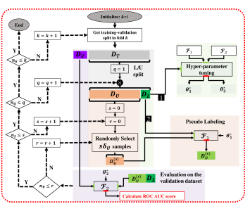
Figure 1: Overview of the proposed semi-supervised pipeline

IV-A Semi-Supervised Models for Pseudo Labeling ($\mathcal{F}_{1}$)

IV-A1 Self-training

Self-training, which dates back to the 1990s [33], has proven to be effective in leveraging unlabeled data to improve supervised classifiers [34, 35, 36, 37, 38]. Self-training works by assigning pseudo labels to unlabeled samples based on the model’s predictions and then training the model iteratively with these pseudo labeled samples. More specifically, for any given base classifier, we learn a model $\mathcal{F}_{1}\in\{\text{SVMR, SVML, GB, DT, kNN}\}$ from the labeled samples in the $\mathbf{D}^{(s)}_{M}$. Then using the learned model, we predict the labels for each $n_{U}^{(s)}$ unlabeled samples to obtain the augmented labeled and pseudo labeled samples, denoted as $\widehat{\mathbf{D}}^{(s)}_{M}$. Algorithm 1 outlines the steps involved in this procedure. Note that the parameter $\delta_{U}$ in this algorithm specifies the number of unlabeled samples (among the $n_{U}^{(s)}$ samples) that will be assigned pseudo-labels in each iteration.

Algorithm 1 Self-Training (for a given $k,q,s,$ and $r$).

1:Input: $\mathbf{D}_{M}^{(s)}$

2:Output: $\widehat{\mathbf{D}}^{(s)}_{M}$

3:Initialize: $[\text{f}:\text{t}]=[1:\delta_{U}]$ $\triangleright$ from sample f to sample t

4:$\quad\qquad\qquad\tilde{\mathbf{X}}_{L}\leftarrow\mathbf{X}_{L},\tilde{\mathbf{Y}}_{L}\leftarrow\mathbf{Y}_{L},\tilde{\mathbf{X}}_{U}\leftarrow\mathbf{X}_{U}[\text{f}:\text{t}]$

5:while t $\leq n_{U}^{(s)}$ do

6:     $\mathcal{F}_{1}:\tilde{\mathbf{Y}}_{L}\leftarrow\tilde{\mathbf{X}}_{L}$ $\triangleright$ Learning the model

7:     $\widehat{\mathbf{Y}}_{U}=\mathcal{F}_{1}(\tilde{\mathbf{X}}_{U})$ $\triangleright$ Pseudo Labeling

8:     $\tilde{\mathbf{X}}_{L}\leftarrow[\tilde{\mathbf{X}}_{L}^{T},\tilde{\mathbf{X}}_{U}^{T}]^{T},\quad\tilde{\mathbf{Y}}_{L}\leftarrow[\tilde{\mathbf{Y}}_{L}^{T},\widehat{\mathbf{Y}}_{U}^{T}]^{T}$ $\triangleright$ Augmentation

9:     $f\leftarrow f+\delta_{U},\quad t\leftarrow t+\delta_{U}$

10:     if t ¿ $n_{U}^{(s)}$:

11:         t $=n_{U}^{(s)}$

12:     $\tilde{\mathbf{X}}_{U}\leftarrow\mathbf{X}_{U}[\text{f}:\text{t}]$

13:end while

14:$\widehat{\mathbf{Y}}_{M}\leftarrow\tilde{\mathbf{Y}}_{L}$

15:Return: $\widehat{\mathbf{D}}^{(s)}_{M}=\{\mathbf{X}_{M},\widehat{\mathbf{Y}}_{M}\}$

IV-A2 Transductive Support Vector Machine (TSVM)

The TSVM approach is a modification of the SVM formulation that addresses the challenge of limited labeled data in classification tasks [39, 40, 31]. The TSVM optimization problem is given by

$$\min_{\mathbf{w},b,\boldsymbol{\eta},\boldsymbol{\zeta},\mathbf{z}}\quad C\left[\sum_{i\in\mathcal{I}_{L}}\eta_{i}+\sum_{j\in\mathcal{I}_{U}}\min(\zeta_{j},z_{j})\right]+\|\mathbf{w}\|$$ (5a)

subject to:

$$y_{i}(\mathbf{w}^{T}x_{i}-b)+\eta_{i}\geq 1,\quad\eta_{i}\geq 0,\quad i\in\mathcal{I}_{L}$$ (5b)

$$\mathbf{w}^{T}x_{i}-b+\zeta_{j}\geq 1,\quad\zeta_{j}\geq 0,\quad j\in\mathcal{I}_{U}$$ (5c)

$$-(\mathbf{w}^{T}x_{i}-b)+z_{j}\geq 1,\quad z_{j}\geq 0,\quad j\in\mathcal{I}_{U}$$ (5d)

where $\mathbf{w}\in\mathbb{R}^{d}$ and $b\in\mathbb{R}$ represent the direction of the decision boundary and the bias (or intercept) term, respectively. It introduces two constraints (i.e., (5c), and (5d)) for each sample in the training dataset calculating the misclassification error as if the sample belongs to one class or the other. The objective function aims to find $\mathbf{w}$ and $b$ that, while maximizing the margin and reducing the misclassification error of labeled samples (i.e., $\boldsymbol{\eta}$), minimize the minimum of these misclassification errors (i.e., $\boldsymbol{\zeta}$ and $\mathbf{z}$). This enables the TSVM to utilize both labeled and unlabeled samples for constructing a precise classification model. Subsequently, it assigns pseudo labels to the unlabeled samples. For brevity, we refer readers to [40] for more comprehensive details.

IV-A3 Label Spreading (LS)

In the realm of semi-supervised learning, label spreading (LS) falls within the category of graph-based semi-supervised (GSSL) models [41]. It involves constructing a graph and inferring labels for unlabeled samples where nodes represent samples and weighted edges reflect similarities. Consider a graph $G_{M}=(\mathcal{V}_{M},\mathcal{W}_{M})$ which is constructed over the mixed labeled and unlabeled training set. Each sample, $x_{i},\forall i\in\mathcal{I}_{L}\cup\mathcal{I}_{U}$, in the $\mathbf{X}_{M}$ can be represented as a graph node, $v_{i}$, i.e., $v_{i}\in\mathcal{V}_{M}\leftarrow x_{i}$. Furthermore, the edge weights matrix defined as $\mathcal{W}_{M}\in\mathbb{R}^{n^{(s)}_{M}\times n^{(s)}_{M}}$. Considering the Euclidean distance $\mathfrak{D}_{ij}=\lvert\lvert x_{i}-x_{j}\lvert\lvert^{2}$, the $i^{\text{th}}$ row and $j^{\text{th}}$ column of $\mathcal{W}_{M}$, denoted as $w_{ij}$, can be obtained as $w_{ij}=\exp({-\mathfrak{D}_{ij}/2\sigma^{2}})$ if $i\neq j$, and $w_{ii}=0$. As a result, the closer the samples are, they will have larger weights. Then the intuition is that similar samples (i.e., with closer distance) have similar labels, and labels propagate from the labeled samples to unlabeled ones through weighted edges where the weights carry the notion of similarity. A pseudo code for the LS algorithm based on [42] is shown in Algorithm. 2. Note that, in updating the labels (line 7 in Algorithm. 2), samples receive information from their neighbors (first term) while preserving their initial information (second term). The parameter $\alpha$ determines the weighting between neighbor-derived information and the sample’s original label information.

Algorithm 2 Label spreading (for a given $k,q,s,$ and $r$).

1:Input: $G=(\mathcal{V},\mathcal{W})\leftarrow\mathbf{D}^{(s)}_{M}=\{\mathbf{X}_{M},\mathbf{Y}_{M}\}$

2:Output: $\widehat{\mathbf{D}}^{(s)}_{M}$

3:Compute: $\mathcal{D}_{ii}=\sum_{j}w_{ij},\quad\forall i\in\mathcal{I}_{L}\cup\mathcal{I}_{U}$

4:Compute: $\mathbf{Z}=\mathcal{D}^{-1/2}\mathcal{W}_{M}\mathcal{D}^{-1/2}$

5:Initialize: $\begin{bmatrix}\mathbf{Y}_{L}|_{t=0}\\ \mathbf{Y}_{U}|_{t=0}\end{bmatrix}\leftarrow\begin{bmatrix}\mathbf{Y}_{L}\\ \mathbf{Y}_{U}\end{bmatrix}$

6:while $\begin{bmatrix}\mathbf{Y}_{L}|_{t}\\ \mathbf{Y}_{U}|_{t}\end{bmatrix}$ converges do $\triangleright$ Based on some threshold

7:     $\begin{bmatrix}\mathbf{Y}_{L}|_{t+1}\\ \mathbf{Y}_{U}|_{t+1}\end{bmatrix}\leftarrow\alpha\mathbf{Z}\begin{bmatrix}\mathbf{Y}_{L}|_{t}\\ \mathbf{Y}_{U}|_{t}\end{bmatrix}+(1-\alpha)\begin{bmatrix}\mathbf{Y}_{L}\\ \mathbf{Y}_{U}\end{bmatrix}$

8:     $t\leftarrow t+1$

9:end while

10:$\widehat{\mathbf{Y}}_{M}\leftarrow\begin{bmatrix}\mathbf{Y}_{L}|_{t}\\ \mathbf{Y}_{U}|_{t}\end{bmatrix}$

11:Return: $\widehat{\mathbf{D}}^{(s)}_{M}=\{\mathbf{X}_{M},\widehat{\mathbf{Y}}_{M}\}$

IV-B Pseudo Labeling Evaluation

Using any of the abovementioned semi-supervised models, we obtain the augmented labeled and pseudo labeled samples, i.e., $\widehat{\mathbf{D}}^{(s)}_{M}$, and learn a new classifier $\mathcal{F}_{2}\in\{\text{SVMR, SVML, GB, DT, kNN}\}$ to assess the model’s performance on the previously unseen validation fold, $\mathbf{D}_{V}$. Within this setting, to ensure a fair comparison among various inductive and transductive semi-supervised approaches, we consider two distinct approaches:

• Approach 1 (Inductive semi-supervised setting):
  $\mathcal{F}_{1}\in\{\text{SVMR, SVML, GB, DT, kNN}\}$ represents the base classifier utilized in self-training for pseudo labeling, and the same type of classifier will be used as $\mathcal{F}_{2}$.

• Approach 2 (Transductive semi-supervised setting):
  $\mathcal{F}_{1}\in\{\text{TSVM, LS}\}$ represents a semi-supervised method used for pseudo labeling, and $\mathcal{F}_{2}\in\{\text{SVMR, SVML, GB, DT, kNN}\}$.

V Simulation Results

In order to investigate the performance of various semi-supervised learning algorithms, we first generate eventful synthetic PMU data, following the procedure described in Section II. Our simulations were carried out on the South-Carolina 500-Bus System [16, 17]. We allow the system to operate normally for $t_{f}=1$ second and then we immediately apply a disturbance. We then run the simulation for an additional $t_{s}=10$ seconds, and record the resulting eventful measurements at the PMU sampling rate of $30$ samples/sec. We assume that 95 buses (which are chosen randomly) of the Carolina 500-bus system are equipped with PMU devices and extract features for each such bus from the $V_{m}$, $V_{a}$, and $F$ channels. We thus collect $N=300$ samples after the start of an event for each channel. We use the modal analysis methodology as outlined in our recent prior work [30] to extract features using modal analysis. In total, we simulated $1827$ events including $500$ LL, $500$ GL, $500$ LT, and $327$ BF events. Figure 2 illustrates the measurements (i.e., $V_{m}$, $V_{a}$, and $F$) recorded from a single PMU after applying LL, GL, LT, and BF events,

Figure 2: PMU measurements

To quantitatively evaluate and compare the performance of different semi-supervised learning algorithms across various scenarios, we employ the area under curve (AUC) of the receiver operator characteristic (ROC). This metric enables the characterization of the accuracy of classification for different discrimination thresholds [43]. The ROC AUC value, which ranges from 0 to 1, provides an estimate of the classifier’s ability to classify events. A value of AUC closer to 1 indicates a better classification performance. For a specified set of parameters $k$, $q$, $s$, and $r$, we evaluate the performance of a given classifier $\mathcal{F}_{2}$ by assessing its ROC-AUC score in predicting event classes within the hold-out fold. This evaluation is based on the model learned from the augmented labeled and pseudo-labeled samples, which are obtained using the pseudo-labeling model $\mathcal{F}_{1}$.

Given that the aim of this study is to provide insight into the robustness of various semi-supervised models, we compare them by evaluating the average, $5^{\text{th}}$ percentile, and $95^{\text{th}}$ percentile of the AUC scores based on the accuracy of the assigned pseudo labels on the unlabeled samples and assess the impact of incorporating the assigned pseudo labels on the accuracy of a generalizable model in predicting the labels of validation samples. We use the $5^{\text{th}}$ percentile of the AUC scores as our primary target performance metric for robustness, as it provides a (nearly) worst-case metric across different selections of the initial labeled and unlabeld samples. That is, if a method yields a high $5^{\text{th}}$ percentile performance, then it is likely to lead to accurate results, even if the initial set of labeled and unlabeled samples are unfavorable.

As discussed in Section IV-B, we investigate and compare the performance of various semi-supervised algorithms, including self-training with different base classifiers (SVML, SVMR, GB, DT, and kNN), TSVM, and LS to assess their effectiveness. In our evaluation process, we take into account $n_{K}=10$ folds and $n_{Q}=30$ random splits of the training samples into labeled and unlabeled subsets. Other simulation parameters are provided in Table. I. As depicted in Figure 3, the comparative performance of diverse classifiers (namely, SVML, SVMR, kNN, DT, and GB) is presented across distinct semi-supervised models (self-training, TSVM, and LS). The outcomes of this analysis highlight that the integration of additional unlabeled samples and the utilization of LS for pseudo labeling surpasses the outcomes achieved by the self-training and TSVM approaches. Moreover, the LS algorithm consistently enhances the performance of all classifiers more robustly. The following subsections provides further insight on the performance of each semi-supervised model.

Parameter	Description	Value
$n_{D}$	Total No. of samples	1827
$n_{K}$	No. of folds	10
$n_{T}$	No. of training samples	1644
$n_{V}$	No. of validation samples	183
$n_{Q}$	No. of random splits of training samples into labeled and unlabeled samples	20
$(B_{\text{min}},B_{\text{max}})$	Class balance range in the labeled samples	(0.2, 0.8)
$n_{L}$	No. of labeled samples	24
$n_{U}$	No. of Unlabeled samples	1620
$\delta_{U}$	No. of unlabeled samples in each step	100
$n_{S}$	Total No. of steps	18
$n_{R}$	No. of random selection of $n^{(s)}_{U}$ samples at each step	20

TABLE I: Parameters used in the simulations for semi-supervised event identification

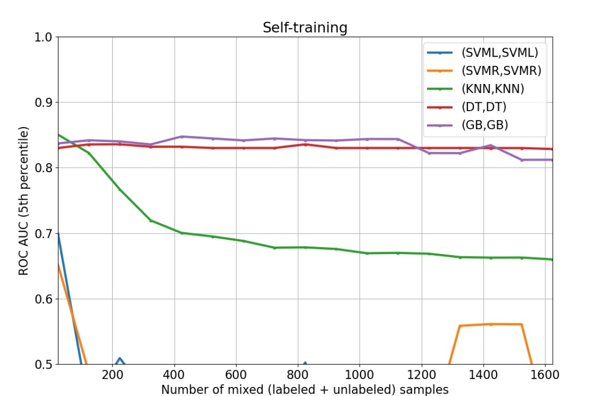
(a)

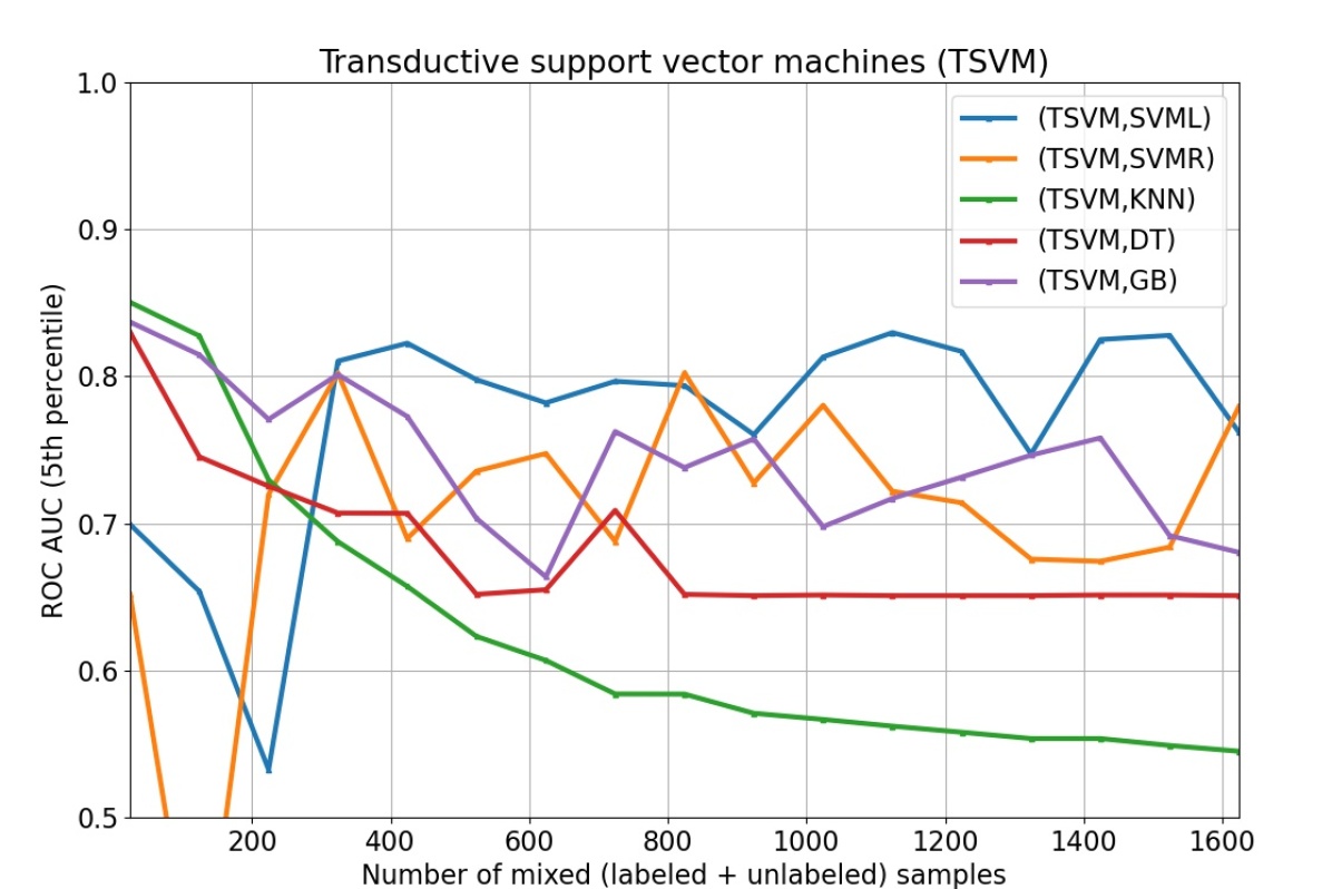
(b)

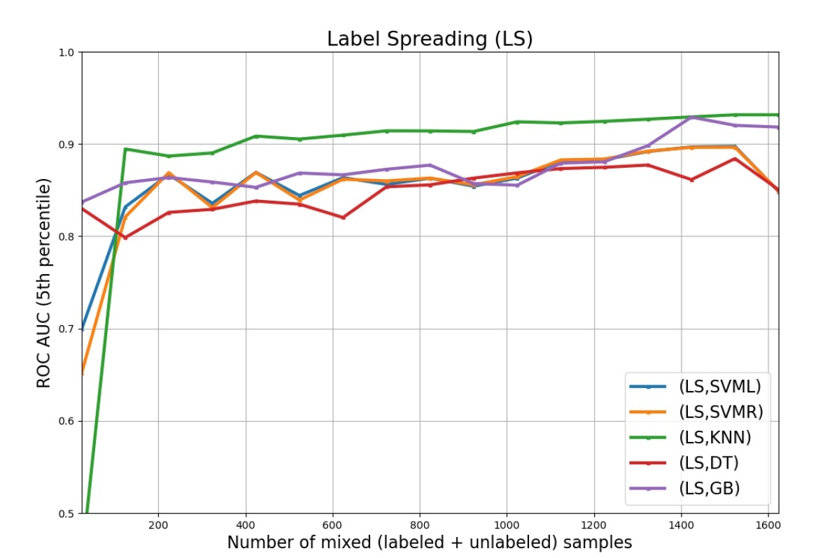
(c)

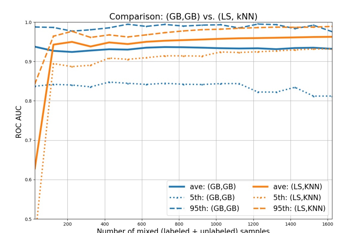
(d)

Figure 3: Comparison between various classifiers based on the Pseudo labels obtained from (a) self-training method with various base classifiers, (b) TSVM, (C) LS. (d) comparison between the (GB, GB) and (LS, kNN).

V-A Approach 1 - Inductive semi-supervised setting

The simulation results for the $5^{\text{th}}$ percentile of the AUC scores of the SVML, SVMR, kNN, DT, and GB classifiers in predicting the labels of validation samples are shown in 3(a). It is clear that using a limited number of labeled samples, results in poor performance for the self-training method when utilizing SVMR, SMVL, and kNN base classifiers. Moreover, the utilization of GB and DT as base classifiers does not necessarily lead to an improvement in event identification accuracy. This primarily arises from the disparity between the pseudo labels and the initial subset of labeled samples. Training with biased and unreliable pseudo labels can result in the accumulation of errors. In essence, this pseudo label bias exacerbates particularly for classes that exhibit poorer behavior, such as when the distribution of labeled samples does not accurately represent the overall distribution of both labeled and unlabeled samples, and is further amplified as self-training continues.

Another noteworthy observation is that self-training employing SVML or SVMR as the classifiers exhibits a high sensitivity to the distribution of both labeled and unlabeled samples. Due to the constraint of having a limited number of labeled samples, these techniques struggle to generate dependable pseudo-label assignments. On the other hand, although self-training with kNN as the base classifier performs better than SVML and SVMR cases, its performance deteriorates as we increase the number of the unlabeled samples. For the self-training with DT and GB base classifiers, it is evident that, although they exhibit more robust performance compared to other types of base classifiers, increasing the number of unlabeled samples does not enhance their performance.

V-B Approach 2 - Transductive semi-supervised setting

The simulation results for the second approach in which TSVM is employed as the semi-supervised method for pseudo-labeling are illustrated in Fig. 3(b). The weak performance of TSVM could be attributed to the specific characteristics of the dataset and the method’s sensitivity to the distribution of labeled and unlabeled samples. If the distribution of these samples is unbalanced or exhibits complex patterns, the TSVM might struggle to accurately capture this distribution. As a result, it could assign inaccurate pseudo labels. Furthermore, it becomes evident that the integration of pseudo-labels acquired through the TSVM algorithm, although yielding an overall performance advantage for SVML and SVMR when compared to the same models utilizing pseudo-labels from the self-training algorithm involving SVMR and SVML, still exhibits substantial sensitivity. This sensitivity is particularly apparent when assessing the $5\%$ AUC scores, highlighting that the accuracy of assigned pseudo-labels remains highly contingent on the initial distribution of labeled and unlabeled samples. This phenomenon is also observable in the diminishing performance of the kNN, GB, and DT classifiers, which, surprisingly, deteriorates to a level worse than their utilization as base classifiers within the self-training framework.

On the contrary, as shown in Fig. 3(c), the results demonstrate that utilizing the augmented labeled and pseudo labeled samples obtained from LS can significantly enhance the performance of event identification, as compared to the self-training and TSVM approaches. Furthermore, the performance of the event identification task improves with a higher number of unlabeled samples, which is particularly significant since labeled eventful PMU data is often scarce in practice. The principal advantage of the LS method, when compared to self-training and TSVM, primarily arises from its ability to leverage information from both labeled and unlabeled samples, as well as their inherent similarities, during the assignment of pseudo labels. For some classifiers (specifically GB and DT), we find that LS improves the $5^{\text{th}}$ percentile line with more unlabeled samples, even though the average performance stays roughly unchanged. On the other hand, for the KNN classifier (as shown in Fig. 3d), the average, $5^{\text{th}}$, and $95^{\text{th}}$ percentile lines all improve with more unlabeled samples. Indeed, LS with KNN seems to be the best overall classifier.

VI Conclusion

Given the practical scenario where a relatively small number of events are labeled in comparison to the total event count, we have introduced a semi-supervised event identification framework to explore the potential benefits of incorporating unlabeled samples in enhancing event identification performance. This framework comprises three core steps: (i) assigning pseudo-labels to unlabeled samples within the training set, which encompasses a mixture of labeled and unlabeled samples, (ii) training a classifier using the augmented set of labeled and pseudo-labeled samples, and (iii) evaluating the classifier’s efficacy on the holdout fold. This proposed pipeline is deployed to scrutinize the effectiveness of three classical semi-supervised methods: self-training, TSVM, and LS. Our simulation results suggests that using a limited number of labeled samples, the self-training and TSVM methods perform poorly and does not necessary improve the accuracy of event identification. The study underscores the robust performance of GB and DT classifiers, though augmenting unlabeled samples does not enhance their performance. Conversely, using the augmented labeled and pseudo-labeled samples obtained from LS consistently outperform the self-training and TSVM approaches, and can significantly improve event identification performance. The performance also improves with a higher number of unlabeled samples, which is important given the scarcity of labeled eventful PMU data.

Nima Taghipourbazargani received his B.Sc. and M.Sc. degrees in Electrical Engineering from Shahid Beheshti University and K.N.Toosi University of Technology, Tehran, Iran in 2015, and 2018, respectively. He is currently pursuing the Ph.D. degree with the School of Electrical, Computer and Energy Engineering, Arizona State University. His research interests include application of machine learning and data science in power systems as well as resilience in critical infrastructure networks.

Lalitha Sankar Lalitha Sankar (Senior Member, IEEE) received the B.Tech. degree from the Indian Institute of Technology, Mumbai, the M.S. degree from the University of Maryland, and the Ph.D. degree from Rutgers University. She is currently a Professor with the School of Electrical, Computer, and Energy Engineering, Arizona State University. She currently leads an NSF HDR institute on data science for electric grid operations. Her research interests include applying information theory and data science to study reliable, responsible, and privacy-protected machine learning as well as cyber security and resilience in critical infrastructure networks. She received the National Science Foundation CAREER Award in 2014, the IEEE Globecom 2011 Best Paper Award for her work on privacy of side-information in multi-user data systems, and the Academic Excellence Award from Rutgers University in 2008.

Oliver Kosut Oliver Kosut (Member, IEEE) received the B.S. degree in electrical engineering and mathematics from the Massachusetts Institute of Technology, Cambridge, MA, USA, in 2004, and the Ph.D. degree in electrical and computer engineering from Cornell University, Ithaca, NY, USA, in 2010. He was a Post-Doctoral Research Associate with the Laboratory for Information and Decision Systems, MIT, from 2010 to 2012. Since 2012, he has been a Faculty Member with the School of Electrical, Computer and Energy Engineering, Arizona State University, Tempe, AZ, USA, where he is currently an Associate Professor. His research interests include information theory, particularly with applications to security and machine learning, and power systems. Professor Kosut received the NSF CAREER Award in 2015.

References

- [1] P. Gao, M. Wang, S. G. Ghiocel, J. H. Chow, B. Fardanesh, and G. Stefopoulos, “Missing Data Recovery by Exploiting Low-Dimensionality in Power System Synchrophasor Measurements,” IEEE Transactions on Power Systems, vol. 31, no. 2, pp. 1006–1013, 2016.
- [2] H. Li, Y. Weng, E. Farantatos, and M. Patel, “An Unsupervised Learning Framework for Event Detection, Type Identification and Localization Using PMUs Without Any Historical Labels,” in 2019 IEEE Power Energy Society General Meeting (PESGM), 2019, pp. 1–5.
- [3] R. Yadav, A. K. Pradhan, and I. Kamwa, “Real-Time Multiple Event Detection and Classification in Power System Using Signal Energy Transformations,” IEEE Transactions on Industrial Informatics, vol. 15, no. 3, pp. 1521–1531, 2019.
- [4] M. He, J. Zhang, and V. Vittal, “Robust Online Dynamic Security Assessment Using Adaptive Ensemble Decision-Tree Learning,” IEEE Transactions on Power Systems, vol. 28, no. 4, pp. 4089–4098, 2013.
- [5] D.-I. Kim, “Complementary Feature Extractions for Event Identification in Power Systems Using Multi-Channel Convolutional Neural Network,” Energies, vol. 14, no. 15, p. 4446, 2021.
- [6] M. Al Karim, M. Chenine, K. Zhu, L. Nordstrom, and L. Nordström, “Synchrophasor-Based Data Mining for Power System Fault Analysis,” in 2012 3rd IEEE PES Innovative Smart Grid Technologies Europe (ISGT Europe), 2012, pp. 1–8.
- [7] M. Biswal, Y. Hao, P. Chen, S. Brahma, H. Cao, and P. De Leon, “Signal Features for Classification of Power System Disturbances using PMU Data,” in 2016 Power Systems Computation Conference (PSCC), 2016, pp. 1–7.
- [8] M. Biswal, S. M. Brahma, and H. Cao, “Supervisory Protection and Automated Event Diagnosis Using PMU Data,” IEEE Transactions on Power Delivery, vol. 31, no. 4, pp. 1855–1863, 2016.
- [9] H. Ren, Z. J. Hou, B. Vyakaranam, H. Wang, and P. Etingov, “Power System Event Classification and Localization Using a Convolutional Neural Network,” Frontiers in Energy Research, vol. 8, 2020. [Online]. Available: https://www.frontiersin.org/article/10.3389/fenrg.2020.607826
- [10] R. Ma, S. Basumallik, and S. Eftekharnejad, “A PMU-Based Data-Driven Approach for Classifying Power System Events Considering Cyberattacks,” IEEE Systems Journal, vol. 14, no. 3, pp. 3558–3569, 2020.
- [11] J. Shi, B. Foggo, and N. Yu, “Power System Event Identification Based on Deep Neural Network With Information Loading,” IEEE Transactions on Power Systems, vol. 36, no. 6, pp. 5622–5632, 2021.
- [12] Z. Li, H. Liu, J. Zhao, T. Bi, and Q. Yang, “Fast Power System Event Identification Using Enhanced LSTM Network With Renewable Energy Integration,” IEEE Transactions on Power Systems, vol. 36, no. 5, pp. 4492–4502, 2021.
- [13] A. J. Wilson, D. R. Reising, R. W. Hay, R. C. Johnson, A. A. Karrar, and T. Daniel Loveless, “Automated identification of electrical disturbance waveforms within an operational smart power grid,” IEEE Transactions on Smart Grid, vol. 11, no. 5, pp. 4380–4389, 2020.
- [14] R. Yadav, S. Raj, and A. K. Pradhan, “Real-time event classification in power system with renewables using kernel density estimation and deep neural network,” IEEE Transactions on Smart Grid, vol. 10, no. 6, pp. 6849–6859, 2019.
- [15] M. Farajzadeh-Zanjani, E. Hallaji, R. Razavi-Far, M. Saif, and M. Parvania, “Adversarial semi-supervised learning for diagnosing faults and attacks in power grids,” IEEE Transactions on Smart Grid, vol. 12, no. 4, pp. 3468–3478, 2021.
- [16] T. Xu, A. B. Birchfield, and T. J. Overbye, “Modeling, tuning, and validating system dynamics in synthetic electric grids,” IEEE Transactions on Power Systems, vol. 33, no. 6, pp. 6501–6509, 2018.
- [17] T. Xu, A. B. Birchfield, K. S. Shetye, and T. J. Overbye, “Creation of synthetic electric grid models for transient stability studies,” in The 10th Bulk Power Systems Dynamics and Control Symposium (IREP 2017), 2017, pp. 1–6.
- [18] F. Yang, Z. Ling, Y. Zhang, X. He, Q. Ai, and R. C. Qiu, “Event detection, localization, and classification based on semi-supervised learning in power grids,” IEEE Transactions on Power Systems, pp. 1–15, 2022.
- [19] Y. Zhou, R. Arghandeh, and C. J. Spanos, “Partial Knowledge Data-Driven Event Detection for Power Distribution Networks,” IEEE Transactions on Smart Grid, vol. 9, no. 5, pp. 5152–5162, 2017.
- [20] J. Ma, Y. V. Makarov, C. H. Miller, and T. B. Nguyen, “Use Multi-Dimensional Ellipsoid to Monitor Dynamic Behavior of Power Systems Based on PMU Measurement,” in 2008 IEEE Power and Energy Society General Meeting - Conversion and Delivery of Electrical Energy in the 21st Century, 2008, pp. 1–8.
- [21] M. Zhou, Y. Wang, A. K. Srivastava, Y. Wu, and P. Banerjee, “Ensemble-Based Algorithm for Synchrophasor Data Anomaly Detection,” IEEE Transactions on Smart Grid, vol. 10, no. 3, pp. 2979–2988, 2019.
- [22] J. Cordova, C. Soto, M. Gilanifar, Y. Zhou, A. Srivastava, and R. Arghandeh, “Shape Preserving Incremental Learning for Power Systems Fault Detection,” IEEE Control Systems Letters, vol. 3, no. 1, pp. 85–90, 2019.
- [23] L. Xie, Y. Chen, and P. R. Kumar, “Dimensionality Reduction of Synchrophasor Data for Early Event Detection: Linearized Analysis,” IEEE Transactions on Power Systems, vol. 29, no. 6, pp. 2784–2794, 2014.
- [24] H. Li, Y. Weng, E. Farantatos, and M. Patel, “A Hybrid Machine Learning Framework for Enhancing PMU-based Event Identification with Limited Labels,” in 2019 International Conference on Smart Grid Synchronized Measurements and Analytics (SGSMA), 2019, pp. 1–8.
- [25] Y.-F. Li and Z.-H. Zhou, “Towards making unlabeled data never hurt,” IEEE Transactions on Pattern Analysis and Machine Intelligence, vol. 37, no. 1, pp. 175–188, 2015.
- [26] H. Li, Y. Weng, E. Farantatos, and M. Patel, “A hybrid machine learning framework for enhancing pmu-based event identification with limited labels,” in 2019 International Conference on Smart Grid Synchronized Measurements and Analytics (SGSMA), 2019, pp. 1–8.
- [27] Y. Yuan, Y. Wang, and Z. Wang, “A data-driven framework for power system event type identification via safe semi-supervised techniques,” IEEE Transactions on Power Systems, pp. 1–12, 2023.
- [28] Y. Zhou, R. Arghandeh, and C. J. Spanos, “Partial knowledge data-driven event detection for power distribution networks,” IEEE Transactions on Smart Grid, vol. 9, no. 5, pp. 5152–5162, 2018.
- [29] Y. Zhou, R. Arghandeh, I. Konstantakopoulos, S. Abdullah, and C. J. Spanos, “Data-driven event detection with partial knowledge: A hidden structure semi-supervised learning method,” in 2016 American Control Conference (ACC), 2016, pp. 5962–5968.
- [30] N. Taghipourbazargani, G. Dasarathy, L. Sankar, and O. Kosut, “A machine learning framework for event identification via modal analysis of pmu data,” IEEE Transactions on Power Systems, pp. 1–12, 2022.
- [31] J. E. van Engelen and H. H. Hoos, “A survey on semi-supervised learning,” Machine Learning, vol. 109, pp. 373 – 440, 2019.
- [32] J. Bergstra and Y. Bengio, “Random search for hyper-parameter optimization.” Journal of machine learning research, vol. 13, no. 2, 2012.
- [33] B. Chen, J. Jiang, X. Wang, J. Wang, and M. Long, “Debiased pseudo labeling in self-training,” arXiv preprint arXiv:2202.07136, 2022.
- [34] D. Yarowsky, “Unsupervised word sense disambiguation rivaling supervised methods,” ACL, 1995.
- [35] R. Rosenfeld, “A maximum entropy approach to unsupervised word sense disambiguation,” ACL, 1996.
- [36] D. McClosky, E. Charniak, and M. Johnson, “Effective self-training for parsing,” in HLT-NAACL, 2006.
- [37] D.-H. Lee, H. S. Xu, X. Zhang, and N. Kwak, “Pseudo-label: The simple and efficient semi-supervised learning method for deep neural networks,” ICML, 2013.
- [38] S. C. Fralick, “Learning to recognize patterns without a teacher,” IEEE Trans. Inf. Theory, vol. 13, pp. 57–64, 1967.
- [39] F. Gieseke, A. Airola, T. Pahikkala, and O. Kramer, “Sparse quasi-newton optimization for semi-supervised support vector machines.” in ICPRAM (1), 2012, pp. 45–54.
- [40] T. Joachims et al., “Transductive inference for text classification using support vector machines,” in Icml, vol. 99, 1999, pp. 200–209.
- [41] Z. Song, X. Yang, Z. Xu, and I. King, “Graph-based semi-supervised learning: A comprehensive review,” IEEE Transactions on Neural Networks and Learning Systems, pp. 1–21, 2022.
- [42] D. Zhou, O. Bousquet, T. Lal, J. Weston, and B. Schölkopf, “Learning with local and global consistency,” Advances in neural information processing systems, vol. 16, 2003.
- [43] R. Zebari, A. Abdulazeez, D. Zeebaree, D. Zebari, and J. Saeed, “A Comprehensive Review of Dimensionality Reduction Techniques for Feature Selection and Feature Extraction,” Journal of Applied Science and Technology Trends, vol. 1, no. 2, pp. 56–70, 2020.