Conformal Temporal Logic Planning using Large Language Models:
Knowing When to Do What and When to Ask for Help

Abstract

This paper addresses a new motion planning problem for mobile robots tasked with accomplishing multiple high-level sub-tasks, expressed using natural language (NL). These sub-tasks should be accomplished in a temporal and logical order. To formally define the overarching mission, we leverage Linear Temporal Logic (LTL) defined over atomic predicates modeling these NL-based sub-tasks. This is in contrast to related planning approaches that define LTL tasks over atomic predicates capturing desired low-level system configurations. Our goal is to design robot plans that satisfy LTL tasks defined over NL-based atomic propositions. A novel technical challenge arising in this setup lies in reasoning about correctness of a robot plan with respect to such LTL-encoded tasks. To address this problem, we propose HERACLEs, a hierarchical conformal natural language planner, that relies on (i) automata theory to determine what NL-specified sub-tasks should be accomplished next to make mission progress; (ii) Large Language Models to design robot plans satisfying these sub-tasks; and (iii) conformal prediction to reason probabilistically about correctness of the designed plans and to determine if external assistance is required. We provide theoretical probabilistic mission satisfaction guarantees as well as extensive comparative experiments on mobile manipulation tasks.

I Introduction

Several motion planning algorithms have been proposed recently that can generate paths satisfying complex high-level tasks expressed as Linear Temporal Logic (LTL) formulas [1, 2, 3, 4, 5, 6, 7, 8, 9, 10, 11, 12, 13, 14, 15]. To define an LTL task, users are required to specify multiple atomic predicates (i.e., Boolean variables) to model desired low-level robot configurations and then couple them using temporal and Boolean operators. However, this demands a significant amount of manual effort, increasing the risk of incorrect formulas, especially for complex requirements. Additionally, complex tasks often result in lengthy LTL formulas, which, in turn, increases the computational cost of designing feasible paths [16]. Natural Language (NL) has also been explored as a more user-friendly means to specify robot missions; however, NL-specified tasks may be characterized by ambiguity. Planning algorithms for NL-based tasks have been proposed recently in [17, 18, 19, 20, 21, 22, 23, 24, 25, 26, 27, 28, 29, 30, 31, 32]; however, unlike LTL planners, they do not offer correctness guarantees, and their performance often deteriorates with increasing task complexity.

To mitigate the limitations mentioned above, we propose an alternative approach to specifying complex high-level robot tasks that combines both LTL and NL. Our focus is on mobile robots tasked with performing multiple high-level semantic sub-tasks (e.g., ’deliver a bottle of water to the table’) within their environments in a temporal and logical order. To formally describe these tasks, we harness the power of LTL. However, a key departure from related LTL planning approaches lies in how we define atomic predicates. In our method, atomic predicates are true when the aforementioned NL-based sub-tasks are accomplished and false otherwise. This stands in contrast to related LTL planning works, discussed earlier, that rely on defining multiple low-level atomic predicates to describe robot movements and actions for the completion of such sub-tasks. As a result, our approach yields shorter LTL formulas and, in turn, to more computationally efficient path design and lower manual effort required to define complex task requirements.

Next, we address the problem of designing robot plans that satisfy LTL tasks defined over NL-based atomic predicates. A novel technical challenge that arises in this setup lies in designing mechanisms (e.g., labeling functions) that can automatically reason about the correctness of plans with respect to such temporal logic specifications.

To address this planning problem, we propose a new planner called HERACLEs, for HiERArchical ConformaL natural languagE planner, relying on a novel integration of existing tools that include task decomposition [33, 34, 35], Large Language Models (LLMs) [36, 37, 38, 39, 40, 41, 42, 43], and conformal prediction (CP) [44, 45, 46, 18, 47]. Specifically, first, we design a high-level task planner that determines what NL-specified sub-task the robot should accomplish next to make mission progress. This planner leverages our prior automaton-based task decomposition algorithm [34]. Then existing LLMs are employed to generate robot plans satisfying the selected NL-specified sub-task. A key challenge here is that LLMs tend to hallucinate, i.e., to confidently generate outputs that are incorrect and possibly unrealistic [48]. This issue becomes more pronounced by potential ambiguity in NL-specified tasks. Thus, to reason about the correctness of the LLM-based plans, inspired by [18, 46], we leverage CP [49]. CP constructs on-the-fly prediction sets that contain the ground-truth/correct robot plan with a user-specified probability. This enables the robot to quantify confidence in its decisions and, therefore, comprehend when to seek for assistance either from human operators, if available, or from the high-level task planner to generate alternative sub-tasks, if any, to make mission progress. The generated plans are executed using existing low-level controllers. We provide extensive comparative experiments on mobile manipulation tasks demonstrating the efficiency of the proposed algorithm.

Contribution: The contribution of the paper can be summarized as follows. First, we propose a novel approach to specify complex high-level robot tasks that aims to bridge the gap between LTL- and NL-based specification methods. Second, we introduce a novel robot planning problem for LTL tasks over NL-based atomic predicates. Third, to address this problem, we provide a planning algorithm that relies on a novel integration of existing tools to design robot plans with probabilistic correctness guarantees. Fourth, we provide extensive comparative experiments demonstrating that the proposed planner outperforms related works.

II Problem Formulation

II-A Robot System and Skills

Consider a mobile robot governed by the following dynamics: ${\mathbf{p}}(t+1)={\mathbf{f}}({\mathbf{p}}(t),{\mathbf{u}}(t))$, where ${\mathbf{p}}(t)\in{\mathcal{P}}\subset\mathbb{R}^{n}$ stands for the state (e.g., position and orientation) of the robot, and ${\mathbf{u}}(t)\in\mathbb{R}^{b}$ stands for control input at discrete time $t$. We assume that the robot state ${\mathbf{p}}(t)$ is known for all time instants $t\geq 0$. The robot has $A>0$ number of abilities/skills collected in a set ${\mathcal{A}}\in\{1,\dots,A\}$. Each skill $a\in{\mathcal{A}}$ is represented as text such as ‘take a picture’, ‘grab’, or ‘move to’. Application of a skill $a$ at an object/region with location ${\mathbf{x}}$ at time $t\geq 0$ is denoted by $s(a,{\mathbf{x}},t)$ or, with slight abuse of notation, when it is clear from the context, by $s(t)$ for brevity. Also, we assume that the robot has access to low level controllers ${\mathbf{u}}(t)$ to apply the skills in ${\mathcal{A}}$. Hereafter, we assume perfect/error-free execution of these capabilities.

II-B Partially Known Semantic Environment

The robot resides in a semantic environment $\Omega\subseteq\mathbb{R}^{d}$, $d\in\{2,3\}$ with fixed, static, and potentially unknown obstacle-free space denoted by $\Omega_{\text{free}}\subseteq\Omega$. We assume that $\Omega_{\text{free}}$ is populated with $M>0$ static semantic objects. Each object $e$ is characterized by its expected location ${\mathbf{x}}_{e}$ and semantic label $c_{e}\in{\mathcal{C}}$, where ${\mathcal{C}}$ is a set collecting all semantic labels that the robot can recognize (e.g., ‘bottle’ or ‘chair’). Notice that the occupied space $\Omega\setminus\Omega_{\text{free}}$ (e.g., walls) may prevent access to semantic objects of interest. We assume that the robot is equipped with (perfect) sensors allowing it to detect obstacles and detect/classify semantic objects.

II-C Task Specification

The robot is responsible for accomplishing a high-level task expressed as an LTL formula [50, 51, 52]. LTL is a formal language that comprises a set of atomic propositions (i.e., Boolean variables), denoted by $\mathcal{AP}$, Boolean operators, (i.e., conjunction $\wedge$, and negation $\neg$), and two temporal operators, next $\bigcirc$ and until $\mathcal{U}$. LTL formulas over a set $\mathcal{AP}$ can be constructed based on the following grammar: $\phi::=\text{true}~{}|~{}\pi~{}|~{}\phi_{1}\wedge\phi_{2}~{}|~{}\neg\phi~{}|~{}\bigcirc\phi~{}|~{}\phi_{1}~{}\mathcal{U}~{}\phi_{2}$, where $\pi\in\mathcal{AP}$. For brevity we abstain from presenting the derivations of other Boolean and temporal operators, e.g., always $\square$, eventually $\lozenge$, implication $\Rightarrow$, which can be found in [16]. For simplicity, hereafter, we restrict our attention to co-safe LTL formulas that is a fragment of LTL that exclude the ‘always’ operator.

We define atomic propositions (APs) so that they are true when a sub-task expressed in natural language (NL) is satisfied, and false otherwise; for example, such a sub-task is ‘deliver a bottle of water to location X’. Each NL-based AP $\pi$, is satisfied by a finite robot trajectory $\tau$, defined as a finite sequence of decisions $s(t)$, i.e., $\tau=s(0),s(1),\dots,s(T)$, for some horizon $T\geq 1$. A robot trajectory $\tau$ satisfying $\pi$ can be generated using existing Large Language Models (LLMs) [30]. We emphasize that the NL-based definition of APs is fundamentally different from related works on LTL planning (see Section I). In these works, APs are defined so that they are true when the system state ${\mathbf{p}}(t)$ belongs to a desired set of states. Then, labeling functions ${\mathcal{L}}:{\mathcal{P}}\rightarrow 2^{\mathcal{AP}}$ can be defined straightforwardly so that they return the APs satisfied at any state ${\mathbf{p}}(t)$. A major challenge arising in the considered setup is the construction of a corresponding labeling function $L$ that can reason about the correctness of plans $\tau$ with respect to the NL-based APs. We address this challenge in Section III-C using conformal prediction.

Co-safe LTL tasks are satisfied by finite robot trajectories $\tau_{\phi}$ defined as $\tau_{\phi}=\tau(0),\tau(1),\dots,\tau(n),\dots,\tau(N)$, where $\tau(n)$ is a finite robot trajectory of horizon $T_{n}$, as defined before. Thus, the total horizon $H$ of the plan $\tau_{\phi}$ is $H=\sum_{n=1}^{N}T_{n}$. We highlight that in $\tau_{\phi}$, the index $n$ is different from the time instants $t\in\{1,\dots,H\}$. In fact, $n\in\{1,\dots,N\}$ is an index, initialized as $n=0$ and increased by $1$ every $T_{n}$ time instants, pointing to the next finite trajectory in $\tau_{\phi}$.

II-D Problem Statement

This paper addresses the following problem (see Ex. II.1):

Problem 1

Given a robot with known dynamics and capabilities (Section II-A), a partially unknown semantic environment $\Omega$ (Section II-B), and an LTL-encoded task $\phi$ constructed using NL-based APs (Section II-C), design (online) a robot path $\tau_{\phi}$ satisfying $\phi$.

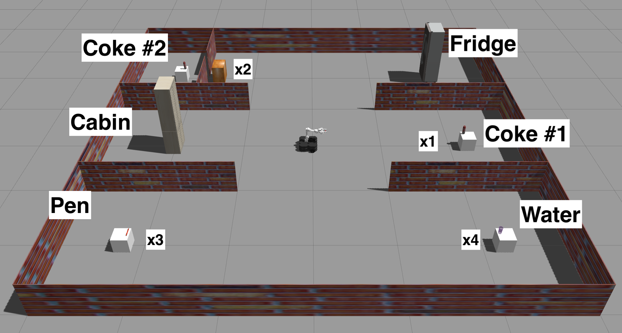
Figure 1: Graphical depiction of a semantic environment with unknown geometric structure.

Example II.1

Consider a robot with skills ${\mathcal{A}}=\{\text{go to},\text{pick up}\}$ residing in an environment shown in Fig. 1. The semantic objects that the robot can recognize are ${\mathcal{C}}=\{\text{Coke},\text{Pen},\text{Water Bottle}\}$. The environment along with the locations of all semantic objects is shown in Fig. 1. The task of the robot $\phi=\Diamond\pi_{2}\wedge(\neg\pi_{1}{\mathcal{U}}\pi_{2})$, where $\pi_{1}$ and $\pi_{2}$ model the sub-tasks ‘Deliver the water bottle to location ${\mathbf{x}}_{3}$’ and $\pi_{2}$ is ‘Deliver a coke to the table at location ${\mathbf{x}}_{3}$’. A plan $\tau_{\phi}$ to satisfy $\phi$ is defined as $\tau_{\phi}=s(\text{go to},{\mathbf{x}}_{1},1),s(\text{grab},{\mathbf{x}}_{1},2),s(\text{go to},{\mathbf{x}}_{3},3),s(\text{go to},{\mathbf{x}}_{4},4),\\ s(\text{grab},{\mathbf{x}}_{4},5),s(\text{go to},{\mathbf{x}}_{3},6)$. Notice that this plan may need to be revised on-the-fly in case an object has been removed from its expected location or the geometric structure of the environment prohibits access to one the semantic objects.

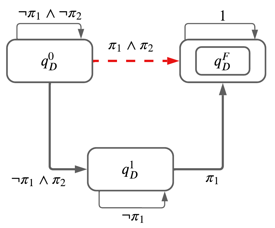
Figure 2: DFA corresponding to $\phi=\Diamond\pi_{2}\wedge(\neg\pi_{1}{\mathcal{U}}\pi_{2})$. $\pi_{1}$ is “Deliver the water bottle to ${\mathbf{x}}_{3}$” and $\pi_{2}$ is “Deliver a Coke to ${\mathbf{x}}_{3}$”. The red dashed edges correspond to an infeasible DFA transition.

III Hierarchical Temporal Logic Planning with Natural Language Instructions

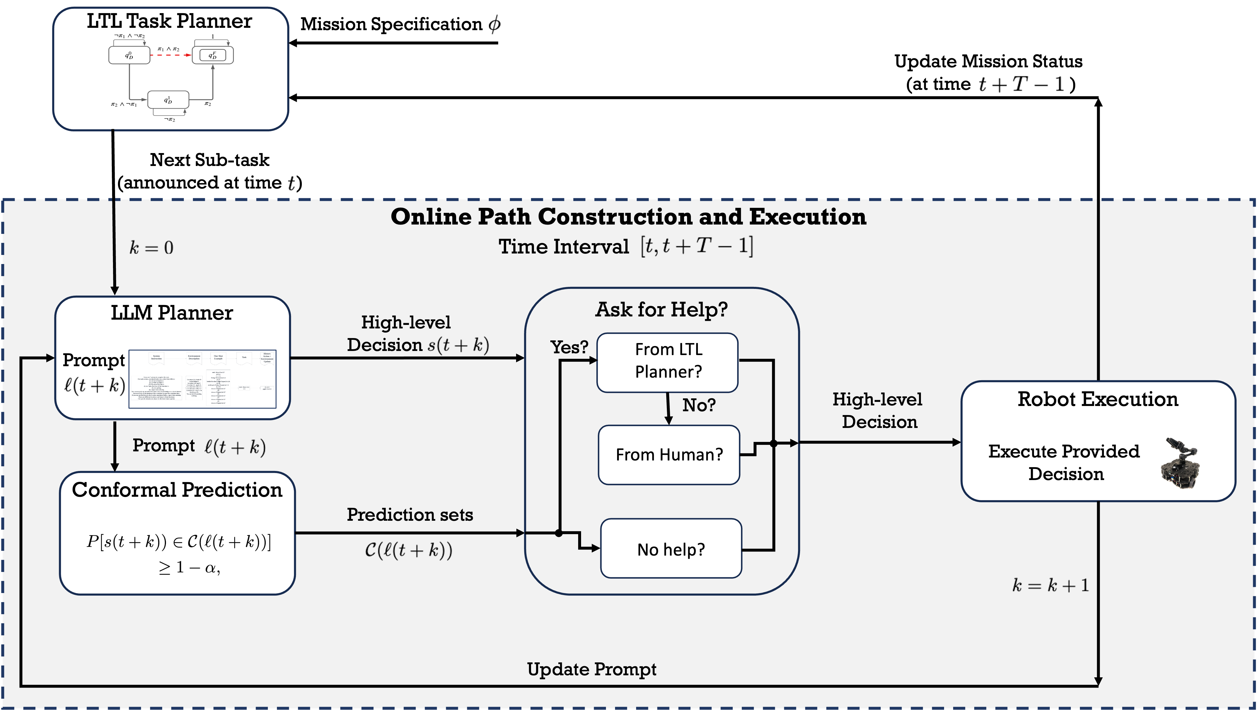
Figure 3: Graphical illustration of HERACLEs. Interaction between the ask-for-help module and the LTL planner is not shown for simplicity (see Section III-D for more details).

In this section, we propose HERACLEs, a new hierarchical planning algorithm to address Problem 1; see Fig. 3. In Section III-A, we provide a high-level LTL-based task planner that, given the current mission status, generates a sub-task and constraints that the robot should accomplish next to make progress towards accomplishing $\phi$. In Section III-B, we discuss how LLMs can be used to design plans $\tau$, defined in Section II-C, satisfying the considered sub-task and constraints. The generated plans $\tau$ are executed using available low-level controllers ${\mathbf{u}}(t)$. In Section III-C, using conformal prediction, we define a labeling function that can probabilistically reason about the correctness of plans $\tau$ with respect to the considered sub-task. In Section III-D we discuss how CP dictates when the robot should seek assistance in order to adapt to unanticipated events that include infeasible sub-tasks (e.g., non-existent objects of interest), ambiguous user-specified NL-based APs, and possibly incorrect LLM-based plans $\tau$.

III-A LTL Task Planner: What to Do Next?

In this section, we present a high-level task planner determining what sub-task the robot should accomplish next to make progress towards accomplishing the LTL task $\phi$. As a first step, we translate $\phi$ into a Deterministic Finite state Automaton (DFA) defined as follows [16]; see Fig. 2.

Definition III.1 (DFA)

A Deterministic Finite state Automaton (DFA) $D$ over $\Sigma=2^{\mathcal{AP}}$ is defined as a tuple $D=\left({\mathcal{Q}}_{D},q_{D}^{0},\Sigma,\delta_{D},q_{D}^{F}\right)$, where ${\mathcal{Q}}_{D}$ is the set of states, $q_{D}^{0}\in{\mathcal{Q}}_{D}$ is the initial state, $\Sigma$ is an alphabet, $\delta_{D}:{\mathcal{Q}}_{D}\times\Sigma\rightarrow{\mathcal{Q}}_{D}$ is a deterministic transition relation, and $q_{D}^{F}\in{\mathcal{Q}}_{D}$ is the accepting/final state.

Next, we introduce notations and definitions that will be used to construct the task planner. First, to interpret a temporal logic formula over a plan $\tau_{\phi}=\tau(0),\tau(1),\dots,\tau(N)$, we use a labeling function $L$ that maps each sub-plan $\tau(n)$ to symbols $\sigma\in\Sigma$. A finite plan $\tau_{\phi}$ satisfies $\phi$ if the word $w=L(\tau(0))L(\tau(1))\dots L(\tau(N))$ yields an accepting DFA run, i.e. if starting from the initial state $q_{D}^{0}$, each element in $w$ yields a DFA transition so that the final state $q_{D}^{F}$ is reached [16]. As discussed in Section II-C, a critical challenge lies in defining the labeling function $L$. We will temporarily assume that such a labeling function has been designed. Its formal construction is deferred to Section III-C. Also, given any two DFA states $q_{D},q_{D}^{\prime}\in{\mathcal{Q}}$ (where $q_{D}\neq q_{D}^{\prime}$ does not necessarily hold), we define the set $\Sigma_{q_{D}\rightarrow q_{D}^{\prime}}\subseteq\Sigma$ that collects all symbols $\sigma\in\Sigma$ that can enable the transition from $q_{D}$ to $q_{D}^{\prime}$, i.e., $\Sigma_{q_{D}\rightarrow q_{D}^{\prime}}=\{\sigma\in\Sigma~{}|~{}q_{D}^{\prime}=\delta(q_{D},\sigma)\}$. Note that a DFA along with sets $\Sigma_{q_{D}\rightarrow q_{D}^{\prime}}$ can be constructed using existing tools such as [53].

In what follows, we present a high-level task planner that leverages the DFA accepting condition to generate sub-tasks, online, that the robot should accomplish next to make mission progress. This planner builds upon our earlier works [33, 34]. First, we define a function over the DFA state-space that captures how far any given DFA state is from the DFA accepting state. To define this function, first, we prune the DFA by removing all infeasible transitions, i.e., transitions that cannot be physically enabled. Specifically, a DFA transition from $q_{D}$ to $q_{D}^{\prime}$ is infeasible if its activation requires the robot to satisfy more than one AP, i.e., accomplish more than one sub-task, simultaneously; a more formal definition can be found in [33, 34]. All symbols $\sigma\in\Sigma$ that are generated only if a robot satisfies more than one AP simultaneously are called infeasible and they are collected in a set $\Sigma^{\text{infeas}}$. Then, we prune the DFA by removing infeasible DFA transitions; see also Fig. 2. Next, we define the function $d:{\mathcal{Q}}_{D}\times{\mathcal{Q}}_{D}\rightarrow\mathbb{N}$ that returns the minimum number of feasible DFA transitions required to reach a state $q_{D}^{\prime}\in{\mathcal{Q}}_{D}$ starting from a state $q_{D}\in{\mathcal{Q}}_{D}$. This function is defined as:

$$d(q_{D},q_{D}^{\prime})=\left\{\begin{array}[]{ll}|SP_{q_{D},q_{D}^{\prime}}|,\mbox{if $SP_{q_{D},q_{D}^{\prime}}$ exists,}\\ \infty,~{}~{}~{}~{}~{}~{}~{}~{}~{}\mbox{otherwise},\end{array}\right.$$ (1)

where $SP_{q_{D},q_{D}^{\prime}}$ denotes the shortest path (in terms of hops) in the pruned DFA from $q_{D}$ to $q_{D}^{\prime}$ and $|SP_{q_{D},q_{D}^{\prime}}|$ stands for its cost (number of hops). Note that if $d(q_{D}^{0},q_{D}^{F})=\infty$, then $\phi$ can not be satisfied since in the pruning process, only the DFA transitions that are impossible to enable are removed.

The function $d$ is used to generate sub-tasks online given the current mission status. Specifically, let $q_{D}(t)$ be the DFA state reached by the robot at time $t$ after applying the first $t$ actions as per $\tau$. This state is initialized as $q_{D}(0)=q_{D}^{0}$. Given $q_{D}(t)$, we compute all DFA states $q_{D}^{\prime}\neq q_{D}(t)$ that are one hop closer to $q_{D}^{F}$ than $q_{D}(t)$ is. These DFA states are collected in a set ${\mathcal{R}}(q_{D}(t))$ defined as follows:

$${\mathcal{R}}(q_{D}(t))=$$ (2)

$$\{q_{D}^{\prime}\in{\mathcal{Q}}_{D}\setminus\{q_{D}(t)\}|d(q_{D}^{\prime},q_{D}^{F})=d(q_{D}(t),q_{D}^{F})-1\}.$$

Among all states in ${\mathcal{R}}(q_{D}(t))$, we select a DFA state denoted by $q_{D}^{\text{next}}$. This state is selected randomly although any user-specified criterion can be used.

Then, given $q_{D}(t)$ and $q_{D}^{\text{next}}$, we construct the set

$$\Sigma_{q_{D}(t)\rightarrow q_{D}^{\text{next}}}^{\text{feas}}=\Sigma_{q_{D}(t)\rightarrow q_{D}^{\text{next}}}\setminus\Sigma^{\text{infeas}},$$ (3)

that collects all feasible symbols that can generate the transition from $q_{D}(t)$ to $q_{D}^{\text{next}}$; see Example III.2. Similarly, we construct the set $\Sigma_{q_{D}(t)\rightarrow q_{D}(t)}^{\text{feas}}$. Notice that this set is empty if there is no self-loop at $q_{D}(t)$. Then, a plan $\tau$ will enable the transition from $q_{D}(t)$ to $q_{D}^{\text{next}}$ at some discrete time step $t^{\prime}\geq t$, if (i) the plan $\tau(t:\bar{t})=s(t),\dots,s(\bar{t})$ satisfies $L(\tau(t:\bar{t}))\in\Sigma_{q_{D}(t)\rightarrow q_{D}(t)}^{\text{feas}}$ and $L(\tau(t:\bar{t}))\notin\Sigma_{q_{D}(t)\rightarrow q_{D}^{\text{next}}}^{\text{feas}}$ for all $\bar{t}\in[t,t^{\prime}-1]$, where $\tau(t:\bar{t})$ denotes the part of the plan $\tau$ from the time instant $t$ until $\bar{t}$, and (ii) the plan $\tau$ satisfies $L(\tau)\in\Sigma_{q_{D}(t)\rightarrow q_{D}^{\text{next}}}^{\text{feas}}$. If there is no self-loop at $q_{D}(t)$ then these conditions should hold for $t^{\prime}=t$. Examples illustrating these conditions can be found in Example III.2.

Among all APs in $\Sigma_{q_{D}(t)\rightarrow q_{D}^{\text{next}}}^{\text{feas}}$ that can be used to satisfy (ii), we select one randomly denoted by $\pi_{\text{next}}$. The NL-based sub-task corresponding to $\pi_{\text{next}}$ along with all sub-tasks in $\Sigma_{q_{D}(t)\rightarrow q_{D}(t)}^{\text{feas}}$ are inputs provided by the high-level LTL planner to the LLM-based planner discussed next.

Example III.2

Consider the DFA in Fig. 2. We have that $\Sigma=\{\pi_{1},\pi_{2},\pi_{1}\pi_{2},\varnothing\}$, where $\varnothing$ is the empty symbol (when no AP is satisfied), and $\Sigma^{\text{infeas}}=\{\pi_{1}\pi_{2}\}$. Also, we have that ${\mathcal{R}}(q_{D}^{0})=\{q_{D}^{1}\}$. Notice that $q_{D}^{F}$ is not included in ${\mathcal{R}}_{q_{D}^{0}}$ as the transition from $q_{D}^{0}$ to $q_{D}^{F}$ is infeasible. Also, we have that $\Sigma_{q_{D}^{0}\rightarrow q_{D}^{1}}^{\text{feas}}=\{\pi_{2}\}$. Similarly, we have that ${\mathcal{R}}(q_{D}^{1})=\{q_{D}^{F}\}$, $\Sigma_{q_{D}^{1}\rightarrow q_{D}^{F}}^{\text{feas}}=\{\pi_{1}\}$. Assume $q_{D}(t)=q_{D}^{1}$ and $q_{D}^{\text{next}}=q_{D}^{F}$. Then, the only option for $\pi_{\text{next}}$ is $\pi_{\text{next}}=\pi_{1}$. In words, this DFA transition will be enabled at $t^{\prime}\geq t$ by a plan $\tau$ of length $t^{\prime}-t$, if the sequence of actions in $\tau$ until the time instant $\bar{t}$, for any $\bar{t}\in[t,t^{\prime}-1]$, does not satisfy $\pi_{\text{next}}$ (condition (ii)) but the entire plan $\tau$ satisfies $\pi_{\text{next}}$ (condition (i)).

III-B LLM Planner: How to Accomplish the Assigned Task?

Next, our goal is to design a plan $\tau$ satisfying conditions (i)-(ii) so that the transition from $q_{D}(t)$ to $q_{D}^{\text{next}}$ is eventually activated. To synthesize $\tau$, we utilize existing LLMs. A key challenge here is that LLMs cannot necessarily break down the conditions (i)-(ii) into low-level instructions that are suitable for robotic execution. For instance, an LLM response to the task ‘bring me a bottle of water’ may be “I need to go to the store and purchase a bottle of water’. Although this response is reasonable, it is not executable by the robot. Therefore, we will inform the LLM that we specifically want the conditions (i)-(ii) to be broken down into sequences of executable robot skills collected in ${\mathcal{A}}$.

Prompt Engineering: To this end, we employ prompt engineering [54]. Prompt engineering provides examples in the context text (‘prompt’) for the LLM specifying the task and the response structure that the model will emulate. The prompt used in this work consists of the following parts. (1) System description that defines the action space determining all possible actions $s(a,{\mathbf{x}},t)$ that the robot can apply and rules that the LLM should always respect in its decision-making process. For instance, in our considered simulations, such rules explicitly determine that the robot cannot grasp an object located in a fridge before opening the fridge door. We observed that explicitly specifying such constraints improved the quality of LLM plans. We additionally require the length of the plan $\tau$ to be less than $T$, where $T\geq 0$ is a user-specified hyperparameter. (2) Environment description that describes the expected locations ${\mathbf{x}}_{e}$ of each semantic object $e$ of interest; (3) Task description that includes the NL definition of the task $\pi_{\text{next}}$ (condition (i)) as well as constraints, if any, imposed by condition (ii), that the robot should respect until $\pi_{\text{next}}$ is satisfied; (4) History of actions & current environment status that includes the sequence of actions, generated by the LLM, that the robot has executed so far towards accomplishing the assigned task. It also includes the current locations of semantic objects that the robot may have sensed or manipulated/moved so far; (5) Response structure describing the desired structure of the LLM output.

Plan Design: In what follows, we describe how we use the above prompt to generate a plan $\tau$ incrementally so that conditions (i)-(ii) are satisfied. The process of designing $\tau$ is converted into a sequence of $T>0$ multiple-choice question-answering problems for the LLM; $T$ essentially determines the horizon $T_{n}$ in Section II-C. Specifically, assume that at time $t$ the robot reaches a DFA state $q_{D}(t)$ and the LTL planner generates the AP $\pi_{\text{next}}$ that needs to be completed next (condition (i)) along with the APs that should not be satisfied in the meantime (condition (ii)). This information is used to generate part (3) in the prompt. Part (4) does not include any textual information at time $t$ as a new sub-task has just been announced. We denote by $\ell(t)$ parts (1)-(5) of the prompt and by $h(t)$ only part (4) of $\ell(t)$ at time $t$. Given $\ell(t)$, the LLM is asked to make a decision $s(a,{\mathbf{x}},t)$ among all available ones included in part (1). For simplicity, we adopt the notation $s(t)$ instead of $s(a,{\mathbf{x}},t)$. We also denote by ${\mathcal{S}}$ all possible decisions $s$ that the robot can make; this set can be constructed offline using the action space ${\mathcal{A}}$ and the available semantic objects. The LLM makes a decision $s(t)$ as follows. Given any $s\in{\mathcal{S}}$, LLMs can provide a score $r(s|\ell(t))$; the higher the score, the more likely the decision $s$ is a valid next step to address the user-specified task $\ell(t)$. Thus, as in [30], we query the model over all potential decisions $s$ and we convert them into a vector of ‘probabilities’ using the softmax function. We denote the softmax score of decision $s$ by $g(s|\ell(t))$. Then, the decision selected at time $t$ is

$$s(t)=\arg\max_{s\in\mathcal{S}}g(s|\ell(t)).$$ (4)

Once $s(t)$ is selected, the robot executes it, the current time step is updated to $t+1$, and the robot internal state ${\mathbf{p}}(t+1)$ is computed. Then, $h(t+1)$ is updated by incorporating perceptual feedback as follows. First, we automatically convert this perceptual feedback into text denoted by $p(t+1)$; recall from Section II that we assume that the robot is equipped with perfect sensors. For instance, when the robot is ${\mathbf{p}}(t+1)$, it may sense an unexpected semantic object of interest at location ${\mathbf{x}}$ or it may not see object $e$ at its expected location ${\mathbf{x}}_{e}$ that was included in environment description in part (2). This sensor feedback will be converted into text of the form ‘object of class $c$ exists in location ${\mathbf{x}}$’ or ‘no object in location ${\mathbf{x}}$’). Then, $h(t+1)$ is updated by including in $h(t)$ the sensor feedback $p(t+1)$ as well as the decision $s(t)$ that was previously taken. With slight abuse of notation, we denote this prompt update by $h(t+1)=h(t)+s(t)+p(t+1)$ where the summation means concatenation of text. This process is repeated for all subsequent time instants $t+k$, $k\in\{2,\dots,T-1\}$. Part (4) is the only part of the prompt that is updated during the time interval $[t+1,t+T-1]$ using the recursive update function $h(t+k)=h(t+k-1)+s(t+k-1)+p(t+k)$ for all $k\in\{1,\dots,T-1\}$.

This process generates a plan

$$\tau=s(t),s(t+1),\dots,s(t+T-1),$$ (5)

of length $T$. At time $t+T$, two steps follow. First, part (2) is updated based on the sensor feedback $p(t+k)$ collected for all $k\in\{1,\dots,T\}$. Part (4) is updated so that it does not include any information. These steps give rise to the prompt $\ell(t+T)$ which is used to compute a plan for the next sub-task that the LTL planner will generate. Concatenation of all plans $\tau$ for the sub-tasks generated by the LTL planner gives rise to the plan $\tau_{\phi}$ (see Section II).

III-C Probabilistic Satisfaction Guarantees for the LTL Mission

As discussed earlier, a key challenge lies in reasoning about correctness of plan $\tau$ with respect to conditions (i)-(ii) (see Section III-A). This is important as it determines if the transition from $q_{D}(t)$ to the desired DFA state $q_{D}^{\text{next}}$ can be enabled after executing the plan $\tau$. To address this challenge, inspired by [18, 46], we utilize an existing conformal prediction (CP) algorithm [49]. CP also allows us to provide probabilistic satisfaction guarantees for $\phi$. Specifically, we utilize CP to compute a prediction set that contains plans that satisfy a given LTL task $\phi$ with high probability. Later, we will show how to use this prediction set to define a labeling function and reason about mission satisfaction.

Single-step Plans: For simplicity, here we focus on LTL formulas $\phi$ that can be satisfied by plans $\tau_{\phi}$ of horizon $H=1$ (see Section II); later we generalize the results for $H\geq 1$. This means that synthesizing $\tau_{\phi}$ requires the LLM to make a single decision $s$. First, we collect a calibration dataset ${\mathcal{M}}=\{(\ell_{\text{calib}}^{i},s_{\text{calib}}^{i})\}_{i=1}^{M}$. We assume that there exists a unique correct decision $s_{\text{calib}}^{i}$ for each $\ell_{\text{calib}}^{i}$. This assumption can be relaxed as in [18]; due to space limitations we abstain from this presentation. Consider a new test data point $\ell_{\text{test}}$ with unknown correct decision $s_{\text{test}}$. CP can generate a prediction set ${\mathcal{C}}(\ell_{\text{test}})$ of decisions $s$ containing the correct one $s_{\text{test}}$ with probability greater than $1-\alpha$, i.e.,

$$P(s_{\text{test}}\in\mathcal{C}(\ell_{\text{test}}))\geq 1-\alpha,$$ (6)

where $\alpha\in[0,1]$ is user-specified. To generate $\mathcal{C}(\ell_{\text{test}})$, CP first uses the LLM’s confidence $g$ (see Section III-B) to compute the set of nonconformity scores $\{r_{i}=1-g(s_{\text{calib}}^{i}~{}|~{}\ell_{\text{calib}}^{i})\}_{i=1}^{M}$ over the calibration set. The higher the score is, the less each data in the calibration set conforms to the data used for training the LLM. Then CP performs calibration by computing the $\frac{(M+1)(1-\alpha)}{M}$ empirical quantile of $r_{1},\dots,r_{M}$ denoted by $q$. Then, it generates prediction set

$$\mathcal{C}(\ell_{\text{test}})=\{s\in{\mathcal{S}}~{}|~{}g(s|\ell_{\text{test}})>1-q\}$$ (7)

includes all labels (i.e., decisions) that the predictor is at least $1-q$ confident in. The generated prediction set ensures the $1-\alpha$ marginal coverage guarantee, mentioned above, holds. By construction of the prediction sets, given an LTL formula $\phi$, the LLM output plan $\tau_{\phi}=\tau=s(t)$ belongs to $\mathcal{C}(\ell_{\text{test}})$ meaning that the satisfaction probability of $\phi$ is greater than $1-\alpha$. A key assumption in CP is that all calibration and test data points are i.i.d. which holds in this setup.

Remark III.3 (Dataset-Conditional Guarantee)

The probabilistic guarantee in (6) is marginal in the sense that the probability is over both the sampling of the calibration set ${\mathcal{M}}$ and the test point $\ell_{\text{test}}$. Thus, a new calibration set will be needed for every single test data point $\ell_{\text{test}}$ to ensure the desired probability $1-\alpha$, which is not practical. Thus, as in [55], we apply the following dataset-conditional guarantee which holds for a fixed calibration set across test data:

$$P(s_{\text{test}}\in\mathcal{C}(\ell_{\text{test}})|{\mathcal{M}})\geq\text{Beta}^{-1}_{M+1-v,v}(\delta),$$ (8)

where $\text{Beta}^{-1}_{M+1-v,v}(\delta)$ denotes the quantile level of $\delta$ in a Beta distribution with $v=\left\lfloor{(M+1)\alpha_{{\mathcal{M}}})}\right\rfloor$. Given a calibration dataset of size $M$ and a small value for $\delta$ ($\delta=0.01$), to achieve the desired coverage guarantee $1-\alpha$ (with probability $1-\delta$), we compute the parameter $\alpha_{{\mathcal{M}}}$ so that $\alpha=1-\text{Beta}^{-1}_{M+1-v,v}(\delta)$.

Multi-step Plans: Next, we generalize the above result to the case where satisfaction of $\phi$ requires plans $\tau_{\phi}$ with $H\geq 1$ decisions selected from ${\mathcal{S}}$. The challenge in this case is that the test points $\{(\ell_{\text{test}}(t+k),s_{\text{test}}(t+k))\}_{k=1}^{T}$ are not independent with each other which violates the exchangeability assumption required to apply CP. The reason is that the test prompts are not independent since the distribution of prompts $\ell_{\text{test}}(t)$ depends on past robot decisions as well as on $\phi$. To address this challenge, as in [18], the key idea is to (i) lift the data to sequences, and (ii) perform calibration at the sequence level using a carefully designed nonconformity score function. First, we construct a calibration dataset as follows. We generate $M\geq 1$ LTL formulas $\phi_{i}$. Each LTL formula is broken into a sequence of $H_{i}\geq 1$ prompts, denoted by:

$$\bar{\ell}_{\text{calib}}^{i}=[\ell_{\text{calib}}^{i}(0),\dots,\ell_{\text{calib}}^{i}(H_{i}-1)],$$ (9)

as discussed in Section III-B. Then for each prompt, we manually construct the corresponding ground truth decisions denoted by

$$\tau_{\phi,\text{calib}}^{i}=s_{\text{calib}}^{i}(0),\dots,s_{\text{calib}}^{i}(H_{i}-1),$$ (10)

This gives rise to the calibration set ${\mathcal{M}}=\{(\bar{\ell}_{\text{calib}}^{i},\tau_{\phi,\text{calib}}^{i})\}_{i=1}^{M}$. As before, we assume that each context $\bar{\ell}_{\text{calib}}^{i}$ has a unique correct plan $\tau_{\phi,\text{calib}}^{i}$. Next, we use the lowest score over the time-steps $1,\dots,H_{i}$ as the score for each sequence $i$ in calibration set, i.e.,

$$\bar{g}(\tau_{\phi,\text{calib}}^{i}~{}|~{}\bar{\ell}_{\text{calib}}^{i})=\min_{t\in\{1,\dots,H_{i}\}}g(s_{\text{calib}}^{i}(t)~{}|~{}\bar{\ell}_{\text{calib}}^{i}(t))$$ (11)

Thus, the non-conformity score of each sequence $i$ is

$$\bar{r}_{i}=1-\bar{g}(\tau_{\phi,\text{calib}}^{i}|\bar{\ell}_{\text{calib}}^{i}).$$ (12)

Consider a new LTL formula $\phi_{\text{test}}$ corresponding to a test data point $\bar{\ell}_{\text{test}}$ with unknown correct label/plan $\tau_{\phi,\text{test}}$ of length $H_{\text{test}}\geq 1$. CP can generate a prediction set $\bar{{\mathcal{C}}}(\bar{\ell}_{\text{test}})$ of plans $\tau_{\phi}$ containing the correct one $\tau_{\phi,\text{test}}$ with high probability i.e.,

$$P(\tau_{\phi,\text{test}}\in\bar{\mathcal{C}}(\bar{\ell}_{\text{test}}))\geq 1-\alpha,$$ (13)

where the prediction set $\bar{\mathcal{C}}(\bar{\ell}_{\text{test}})$ is defined as

$$\bar{\mathcal{C}}(\bar{\ell}_{\text{test}})=\{\tau~{}|~{}\bar{g}(\tau|\ell_{\text{test}})>1-\bar{q}\},$$ (14)

where $\bar{q}$ is the $\frac{(M+1)(1-\alpha)}{M}$ empirical quantile of $\bar{r}_{1},\dots,\bar{r}_{M}$. The generated prediction set ensures that the coverage guarantee in (13) holds. By construction of the prediction sets, the plan $\tau_{\phi}$ generated by the LLM belongs to $\bar{\mathcal{C}}(\bar{\ell}_{\text{test}})$.

Causal Construction of the Prediction Set: Observe that $\bar{\mathcal{C}}(\bar{\ell}_{\text{test}})$ is constructed after the entire sequence $\bar{\ell}_{\text{test}}=\ell_{\text{test}}(0),\dots,\ell_{\text{test}}(H_{\text{test}}-1)$ is observed. However, at every (test) time $t\in\{1,\dots,H_{\text{test}}\}$, the robot observes only $\ell_{\text{test}}(t)$ and not the whole sequence. Thus, the prediction set needs to be constructed in a causal manner using only the current and past information. Thus, at every (test) time step $t$, we construct the causal prediction set $\mathcal{C}(\ell_{\text{test}}(t)))=\{s~{}|~{}g(s|\ell(t)))>1-\bar{q}\}$. Alternatively, $\mathcal{C}(\ell(t)))$ can be constructed using the RAPs approach that can result in smaller prediction sets [49]; see Section IV-C. Then, the causal prediction set associated with $\bar{\ell}_{\text{test}}$ is defined as

$$\mathcal{C}(\bar{\ell}_{\text{test}})=\mathcal{C}(\ell(0)))\times\mathcal{C}(\ell(1)))\dots\mathcal{C}(\ell(H_{\text{test}}))).$$ (15)

As shown in [18], $\mathcal{C}(\bar{\ell}_{\text{test}})$ and $\bar{\mathcal{C}}(\bar{\ell}_{\text{test}})$, it hold that $\bar{\mathcal{C}}(\bar{\ell}_{\text{test}})=\mathcal{C}(\bar{\ell}_{\text{test}})$.

Probabilistic LTL Satisfaction Guarantees: Using the above CP framework, we can state the following result.

Theorem III.4

With probability $1-\delta$ over the sampling of the calibration set ${\mathcal{M}}$, the completion rate over new (but i.i.d.) test scenarios $\phi_{\text{test}}$ is at least $1-\alpha$, if $|\mathcal{C}(\ell_{\text{test}}(t)))|=1$, for all $t\in\{1,\dots,H_{\text{test}}\}$ i.e., $\mathbb{P}(\tau_{\phi,{\text{test}}}\models\phi_{\text{test}})\geq 1-\alpha$, where $\tau_{\phi,{\text{test}}}$ is generated by HERACLEs.

Proof:

This result follows directly from (13). If $|\mathcal{C}(\ell_{\text{test}}(t)))|=1$, for all $t\in\{1,\dots,H_{\text{test}}\}$, then, since $\mathcal{C}(\bar{\ell}_{\text{test}})=\bar{\mathcal{C}}(\bar{\ell}_{\text{test}})$, we have that (13) is equivalent to $\mathbb{P}(\tau_{\phi,{\text{test}}}\models\phi_{\text{test}})\geq 1-\alpha$ (with probability $1-\delta$ as discussed in Remark III.3), completing the proof. ∎

Labeling Function: Theorem III.4 motivates the following definition for the labeling function $L$:

$$L(\tau|\bar{\ell}_{\text{test}})=\begin{cases}\text{T}&\text{if $|{\mathcal{C}}(\ell_{\text{test}}(t+k))|=1,\forall k\in\{1,\dots,T-1\}$}\\ \text{F}&\text{otherwise},\end{cases}$$

where T and F stand for the logical true and false, respectively. In words, we say that $\tau$ enables the transition from $q_{D}(t)$ to $q_{D}^{\text{next}}$ only if the cardinality of $\mathcal{C}(\ell_{\text{test}}(t+k)))$ is $1$, for all $k\in\{1,\dots,T-1\}$. This definition ensures that $\tau_{\phi,\text{test}}$ will be constructed using plans $\tau$ with singleton causal prediction sets so that Theorem III.4 holds.

Otherwise, if $|\mathcal{C}(\ell_{\text{test}}(t+k)))|>1$ for at least one $k\in\{1,\dots,T\}$, then $L(\tau|\bar{\ell}_{\text{test}})=F$ and $\tau$ does not enable the required DFA transition.

III-D When to Seek for Assistance?

Assume that there exists at least one $k\in\{1,\dots,T\}$ so that $|\mathcal{C}(\ell_{\text{test}}(t+k)))|>1$. In this case, the robot asks for help in order to proceed; see Fig. 3. This assistance request and response occurs as follows. First, the robot requests a new sub-task from the LTL planner to make mission progress. To this end, first $\pi_{\text{next}}$ is removed from $\Sigma_{q_{D}(t)\rightarrow q_{D}^{\text{next}}}^{\text{feas}}$, i.e.,

$$\Sigma_{q_{D}(t)\rightarrow q_{D}^{\text{next}}}^{\text{feas}}=\Sigma_{q_{D}(t)\rightarrow q_{D}^{\text{next}}}^{\text{feas}}\setminus\{\pi_{\text{next}}\}.$$ (16)

Then, the LTL planner selects a new AP from $\Sigma_{q_{D}(t)\rightarrow q_{D}^{\text{next}}}^{\text{feas}}$ and the process of generating a feasible plan $\tau$ follows (Section III-B). If there are no other available APs in $\Sigma_{q_{D}(t)\rightarrow q_{D}^{\text{next}}}^{\text{feas}}$, i.e.,

$$\Sigma_{q_{D}(t)\rightarrow q_{D}^{\text{next}}}^{\text{feas}}=\emptyset,$$ (17)

then $q_{D}^{\text{next}}$ is removed from ${\mathcal{R}}(q_{D}(t))$, i.e.,

$${\mathcal{R}}(q_{D}(t))={\mathcal{R}}(q_{D}(t))\setminus\{q_{D}^{\text{next}}\},$$ (18)

and a new DFA state $q_{D}^{\text{next}}$ is selected from the resulting set ${\mathcal{R}}(q_{D}(t))$. Then, an AP $\pi_{\text{next}}$ is selected (Section III-A) and the process of designing a plan $\tau$ follows (Section III-B). If there are no available states in ${\mathcal{R}}(q_{D}(t))$, i.e., ${\mathcal{R}}(q_{D}(t))=\emptyset$, then the LTL planner fails to provide assistance. In this case, the robot asks for help from a human operator. Specifically, first a DFA state $q_{D}^{\text{next}}$ is selected from the original set ${\mathcal{R}}(q_{D}(t))$. Then, the robot returns to the user the prompts $\ell_{\text{test}}(t+k)$ for which it holds $|\mathcal{C}(\ell_{\text{test}}(t+k)))|>1$, waiting for the human operator to select the correct decision $s(t+k)$. We emphasize that help from the LTL planner can also be requested if the robot cannot physically execute $s(t)$ (e.g., grabbing a non-reachable or non-existent object) regardless of the prediction set size, as e.g., in [33, 34]; see Sec. IV-B.

IV Numerical Experiments

In this section, we provide extensive comparative experiments to demonstrate HERACLEs. In Section IV-A, we compare the proposed planner against existing LLM planners that require the task description exclusively in NL. These experiments show that the performance gap between baselines and HERACLEs increases significantly as task complexity increases. In Section IV-B, we illustrate the proposed planner on mobile manipulation tasks; see the supplemental material. To demonstrate the seek-for-assistance module we consider unknown environments and APs with ambiguous instructions. In Section IV-C, we provide additional comparisons showing how various choices of CP algorithm [49, 18] can affect the number of times assistance is requested. Finally, in Section IV-D, we compare the effect of defining NL-based predicates against system-based predicates, being used widely in related LTL planning works, on the DFA size. In all case studies, we pick GPT-3.5 [39] as the LLM. Videos can be found on ltl-llm.github.io.

IV-A Comparisons against LLM planners with NL Tasks

Setup: We consider the following semantic objects $\mathcal{C}=\{\text{Coke, Pen, Water Bottle, Apple, Tin Can}\}$ that can be recognized by the robot. The environment is populated with two cans of Coke, one water bottle, one pen, one tin can, and one apple. The water bottle is inside the fridge and the tin can is inside a drawer. Thus, grabbing e.g., the pen requires the robot to first open the drawer if it is closed. The status of these containers (open or closed) is not known a-priori and, therefore, not included in the environment description in $\ell(t)$. Instead, it can be provided online through sensor feedback as described in Section III-B. For simplicity, here we assume that the expected locations of all objects are accurate and the obstacle-free space is known. The latter ensures that robot knows beforehand if there are any objects being blocked by surrounding obstacles. The action space ${\mathcal{A}}$ is defined as in Table I includes $6$ actions. The action ‘do nothing’ in ${\mathcal{A}}$ is useful when a sub-task can be accomplished in less than $T$ time steps while the action ‘report missing item’ is desired when the robot realizes, through sensor feedback $p(t)$, that objects that are not at their expected locations. This action can be used e.g., to notify a user about missing objects. The action ‘do nothing’ is useful when a sub-task can be accomplished in less than $T$ time steps while the action ‘report missing item’ is desired when the robot realizes, through sensor feedback $p(t)$, that objects that are not at their expected locations. This action can be used e.g., to notify a user about missing objects. Given a prompt $\ell(t)$, the number of choices/decisions $s$ that the LLM can pick from is $|{\mathcal{S}}|=18$. Recall that this set is constructed using ${\mathcal{A}}$ and all objects/locations in the environment where the actions in ${\mathcal{A}}$ can be applied. We select $T=7$ for all sub-tasks generated by the LTL planner.

Symbol	Explanation
(1, X)	Go to location X
(2, X)	Pick up object X
(3)	Put down object
(4, X)	Open the door of the container X
(5)	Do nothing
(6)	Report item missing/Failure

TABLE I: Action space space used in Section IV. The left column shows how each action in encoded in the prompt and the right one provides its explanation. $X$ is a variable referring to An object/region/container selected by the LLM. The plans $\tau_{\phi}$ are finite sequences of these actions.

Baseline: As a baseline for our experiments, we employ saycan, a recently proposed LLM-based planner [30], that requires the task to be fully described using NL. Thus, we manually convert LTL tasks into NL ones, which are then used as inputs for [30]. We compare the accuracy of HERACLEs and saycan over $111$ case studies. For accuracy, we report the percentage of cases where a planner generates a plan that accomplishes the original task. To make comparisons fair we have applied the algorithms under the following settings: (i) Both saycan and HERACLEs select a decision from the same set ${\mathcal{S}}$. (ii) We remove altogether the CP component from our planner (since it does not exist in [30]). This implies that the labeling function $L$ in our planner is defined naively in the sense that given any plan generated by the LLM, the desired DFA transition is assumed to be enabled. This also implies that the CP-module in Fig. 3 will never trigger an assistance request. (iii) We require the baseline to complete the plan within $T\times K$ steps, where $K$ is the number of predicates/sub-tasks in $\phi$. We classify the considered case studies into the following three categories:

Case Study I (Easy): We consider $25$ LTL formulas of the form $\phi=\Diamond\pi_{1}$ where $\pi_{1}$ is defined as ‘Move object $c$ to location ${\mathbf{x}}$” for various objects $c\in{\mathcal{C}}$ and locations ${\mathbf{x}}$. We manually translate such formulas into NL as ‘Eventually move object $c$ to location ${\mathbf{x}}$’. The accuracy of the proposed planner was $100\%$ while the baseline managed to design correct plans in $24$ cases, i.e., its accuracy was $96\%$. To compute this accuracy, we manually check the correctness of the designed plans. Notice that the performance of both planners is comparable due to the task simplicity.

Case Study II (Medium): For medium tasks, we consider $15$ LTL formulas defined as either $\phi_{1}=\Diamond\pi_{1}\wedge\Diamond\pi_{2}$ or $\phi_{2}=\Diamond\pi_{1}\wedge\Diamond\pi_{2}\wedge(\neg\pi_{1}{\mathcal{U}}\pi_{2})$. The task $\phi_{1}$ requires to eventually complete the sub-tasks $\pi_{1}$ and $\pi_{2}$ in any order while $\pi_{2}$ requires $\pi_{2}$ to be completed strictly before $\pi_{1}$. The APs $\pi_{1}$ and $\pi_{2}$ are defined as before. The accuracy of our planner and the baseline is $93.3\%$ and $40\%$, respectively. Observe that the performance of the baseline drops as temporal and/or logical requirements are incorporated into the task description.

Case Study III (Hard): As for hard tasks, we consider $71$ LTL formulas defined over at least $4$ atomic predicates. Two examples of such LTL formulas are: $\phi_{1}=\Diamond\pi_{1}\wedge\Diamond\pi_{2}\wedge\Diamond\pi_{3}\wedge\Diamond\pi_{4}\wedge(\neg\pi_{4}{\mathcal{U}}\pi_{1})$ and $\phi_{2}=\Diamond\pi_{1}\wedge\Diamond\pi_{2}\wedge\Diamond\pi_{3}\wedge(\neg\pi_{3}{\mathcal{U}}\pi_{2})\wedge\Diamond\pi_{5}\wedge(\neg\pi_{2}{\mathcal{U}}\pi_{5})\wedge(\neg\pi_{5}{\mathcal{U}}\pi_{1})\wedge\Diamond\pi_{4}$. For instance, $\phi$ requires the robot to accomplish $\pi_{1}$, $\pi_{2}$, $\pi_{3}$ and $\pi_{4}$ in any order as long as $\pi_{1}$ is executed before $\pi_{4}$. The predicates are defined as before. The accuracy of our planner and the baseline is $93\%$ and $14.08\%$. Mistakes made by our planner were mostly because the LLM asked the robot to move to the wrong location to pick up a desired object or the LLM requested the robot to pick up an object inside a closed container without first opening it.

Observe that the performance gap increases significantly as the task complexity increases. Also, notice that the performance of the proposed planner does not change significantly across the considered case studies. The reason is that it decomposes the overall planning problem into smaller ones that can be handled efficiently by the LLM. This is in contrast to the baseline where the LLM is responsible for generating plans directly for the original long-horizon task. In the above case studies, the average runtime required for the LTL and the LLM planner to generate a subtask and a decision was $2.7\times 10^{-5}$ and $1.2$ secs, respectively.

IV-B Robotic Platform Demonstrations

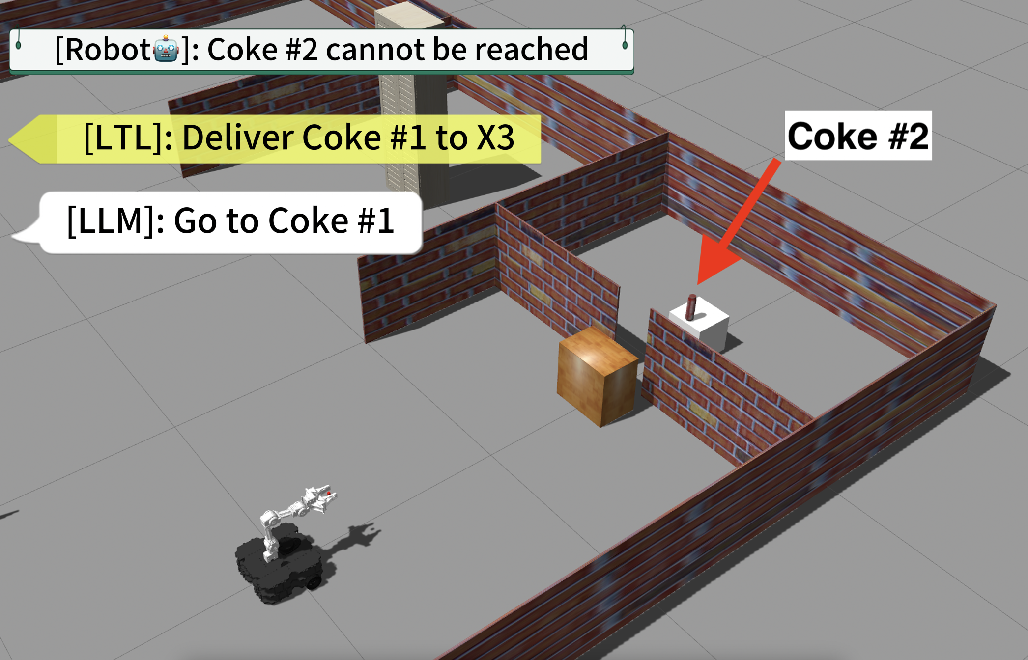
(a) Heading towards Coke #2

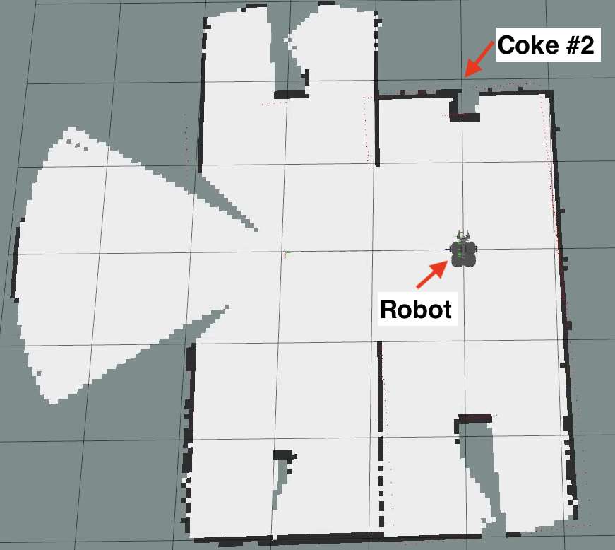
(b) Online-learned Occupancy Grid Map.

Figure 4: As the robot navigates towards Coke #2 (Fig. 4(a)), it builds the occupancy grid map of the environment (Fig. 4(b)) allowing it to realize that Coke #2 is not accessible. Once this happens, the robot asks for help from the LTL planner.

In this section, we demonstrate HERACLEs, using ROS/Gazebo [56], on mobile manipulation tasks using a ground robot (Turtlebot3 Waffle Pi robot [57, 58]) equipped with a manipulator arm with 4 DOFs (OpenManipulator-X[59]). Unlike Section IV-A, the robot is allowed to ask for help, whenever needed, as determined by CP with $\alpha=0.05$. The robot can recognize the following objects ${\mathcal{C}}=${Coke, Pen, Water Bottle}. Particularly, there are two cans of Coke, one water bottle, and one pen (see Fig. 1). The robot knows the exact position of each object but the obstacle-free space of the environment is unknown. As a result, the robot is not aware a priori if there is any object that cannot be reached due to blocking obstacles. We use existing navigation and sensing stacks [60] for Turtlebots as well as the MoveIt![61] toolbox for manipulation control.

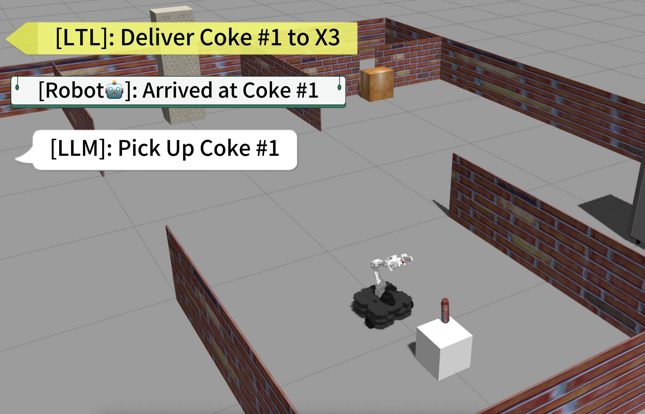
(a) Heading towards Coke #1.

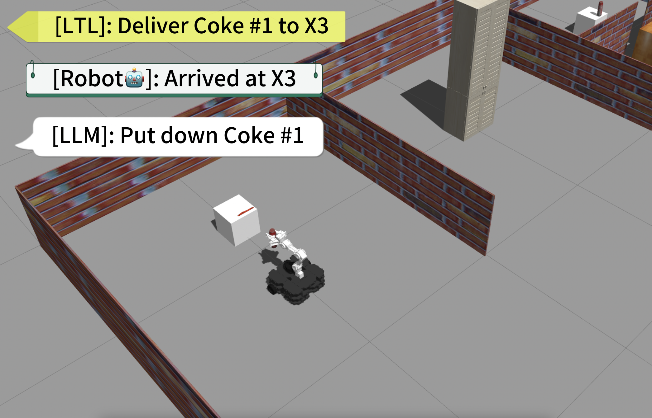
(b) Putting down Coke #1 at ${\mathbf{x}}_{3}$.

Figure 5: Once the robot arrives at the location of Coke #1, the LLM planner generates a new decision asking the robot to pick up the Coke (Fig. 5(a)). Once it is picked, the LLM requests the robot to move to location ${\mathbf{x}}_{3}$ and then put down the coke (Fig. 5(b)). After this step, the mission is completed.

Case Study I: Consider the task $\phi=\Diamond(\pi_{1}\vee\pi_{2})$ where $\pi_{1}$ means ‘Deliver Coke #1 to ${\mathbf{x}}_{3}$’ and $\pi_{2}$ means ‘Deliver Coke #2 to ${\mathbf{x}}_{3}$. This task requires either Coke #1 or #2 to be delivered to ${\mathbf{x}}_{3}$. Initially, the LTL planner selects $\pi_{2}$ as $\pi_{\text{next}}$. As the robot navigates the environment to reach Coke #2, it builds an occupancy grid map of the environment that is used, as in [33], to reason about whether the object is blocked by surrounded obstacles or not. Once the robot realizes that Coke #2 is not reachable (see Fig. 4), it requests help from the LTL planner. In response to that request, the LTL planner generates an alternative sub-task, modeled by $\pi_{1}$, that is eventually successfully accomplished by the robot (see Fig. 5). Assistance from a human operator was never requested in this case study.

Case Study II: Consider the task $\phi=\Diamond\pi_{1}\wedge\Diamond\pi_{2}$ where both $\pi_{1}$ and $\pi_{2}$ mean ‘Bring a drink to location LC’. Observe that these APs are ambiguous as both water and Coke qualify as drinks. Once the LTL planner generates the sub-task $\pi_{1}$, the LLM selects the action ‘go to the Coke #1 location’. However, the prediction set includes two actions ‘go to the water bottle location’ and ‘go to the Coke #1 location’. We note here that, interestingly, we did not specify in the prompt that both water and coke qualify as drinks. In this case, the robot asks for help from the LTL planner. The LTL planner cannot provide assistance as there are no alternative sub-tasks to make mission progress. Thus, the robot next seeks help from a user. Once the user selects the desired action and $\pi_{1}$ is satisfied, the LTL planner generates the next sub-task $\pi_{2}$ and the above process repeats.

IV-C Conformal Prediction Comparisons

The prediction sets can be constructed using existing CP algorithms; see Section III-C. In our implementation, we have employed RAPS [49] as opposed to the ‘vanilla’ CP algorithm [62]. We note that [46, 18] employ the ‘vanilla’ CP algorithm. In what follows, we demonstrate how the choice of the CP affects HERACLEs. To apply CP, we construct a calibration dataset with $M=70$ datapoints. We use $\delta=0.01$ and $\alpha_{{\mathcal{M}}}=0.00842$ to achieve the desired $\alpha=0.05$ satisfaction guarantee. We also construct a test dataset that includes the $111$ case studies considered in Section IV-A. Among the $111$ case studies, $75$ and $70$ of them correspond to plans $\tau_{\phi}$ associated with singleton prediction sets using RAPS and vanilla CP, respectively. This is expected as RAPS can generate smaller prediction sets [49]. Thus, employing RAPS can minimize the number of times assistance will be requested. Among the singleton-prediction-set plans, $100\%$ and $97.2\%$ of them, respectively, satisfy their corresponding LTL tasks. Observe that these percentages are greater than $95\%$ as expected (with probability greater than $1-\delta=0.99$), since $1-\alpha=0.95$. The average runtime to construct a prediction set using RAPS and vanilla CP was $3.35\times 10^{-5}$ and $1.26\times 10^{-6}$ secs, respectively.

IV-D Effect of Task Specification on the Automaton Size

In this section, we demonstrate that the proposed task specification approach using NL-based predicates results in shorter LTL formulas compared to related works that define atomic predicates directly over the system state ${\mathbf{p}}(t)$; Section I. Shorter LTL formulas result in smaller automata size which, in turn, results in more computationally efficient plan synthesis. For instance, consider the LTL formula $\phi=\Diamond(\pi_{1})$ where the NL-based predicate $\pi_{1}$ is true if the robot delivers a bottle of water to location $A$. This formula corresponds to a DFA with $2$ states and 3 edges. Using system-based predicates, the same task can be written as $\phi=\Diamond(\pi_{1}^{\prime}\wedge(\Diamond\pi_{2}^{\prime}\wedge(\Diamond\pi_{3}^{\prime}\wedge(\Diamond\pi_{4}^{\prime}))))$ where $\pi_{1}^{\prime}$ is true if the robot position is close enough to the bottle of water, $\pi_{2}^{\prime}$ is true if the robot grabs the bottle successfully, $\pi_{3}^{\prime}$ is true if the robot position is close enough to location $A$, and $\pi_{4}^{\prime}$ is true if the robot puts down the water bottle successfully. This formula corresponds to DFA with $5$ states and $15$ edges. The difference in the automaton size becomes more pronounced as task complexity increases. For instance, consider the NL-based LTL formula $\phi=\Diamond(\pi_{1})\wedge\Diamond(\pi_{2})$ where both $\pi_{1}$ and $\pi_{2}$ model delivery tasks as before. This formula corresponds to a DFA with $4$ states and $9$ edges. Expressing the same task using system-based predicates as before would result in a DFA with $25$ states and $225$ edges.

V Conclusion

In this paper, we propose HERACLEs, a new robot planner for LTL tasks defined over NL-based APs. Our future work will focus on extending the planner to multi-robot systems as well as accounting for imperfect execution of robot skills.

References

- [1] H. Kress-Gazit, G. E. Fainekos, and G. J. Pappas, “Where’s waldo? sensor-based temporal logic motion planning,” in IEEE International Conference on Robotics and Automation, 2007, pp. 3116–3121.
- [2] E. Plaku, L. E. Kavraki, and M. Y. Vardi, “Motion planning with dynamics by a synergistic combination of layers of planning,” IEEE Transactions on Robotics, vol. 26, no. 3, pp. 469–482, 2010.
- [3] S. L. Smith, J. Tumova, C. Belta, and D. Rus, “Optimal path planning for surveillance with temporal-logic constraints,” The International Journal of Robotics Research, vol. 30, no. 14, pp. 1695–1708, 2011.
- [4] J. Tumova and D. V. Dimarogonas, “Multi-agent planning under local ltl specifications and event-based synchronization,” Automatica, vol. 70, pp. 239–248, 2016.
- [5] Y. Chen, X. C. Ding, A. Stefanescu, and C. Belta, “Formal approach to the deployment of distributed robotic teams,” IEEE Transactions on Robotics, vol. 28, no. 1, pp. 158–171, 2012.
- [6] A. Ulusoy, S. L. Smith, and C. Belta, “Optimal multi-robot path planning with ltl constraints: guaranteeing correctness through synchronization,” in Distributed Autonomous Robotic Systems. Springer, 2014, pp. 337–351.
- [7] E. Plaku and S. Karaman, “Motion planning with temporal-logic specifications: Progress and challenges,” AI communications, vol. 29, no. 1, pp. 151–162, 2016.
- [8] Y. Shoukry, P. Nuzzo, A. Balkan, I. Saha, A. L. Sangiovanni-Vincentelli, S. A. Seshia, G. J. Pappas, and P. Tabuada, “Linear temporal logic motion planning for teams of underactuated robots using satisfiability modulo convex programming,” in IEEE 56th Conference on Decision and Control, December 2017, pp. 1132–1137.
- [9] X. Sun and Y. Shoukry, “Neurosymbolic motion and task planning for linear temporal logic tasks,” arXiv preprint arXiv:2210.05180, 2022.
- [10] Y. Kantaros and M. M. Zavlanos, “Stylus*: A temporal logic optimal control synthesis algorithm for large-scale multi-robot systems,” The International Journal of Robotics Research, vol. 39, no. 7, pp. 812–836, 2020.
- [11] C. I. Vasile and C. Belta, “Sampling-based temporal logic path planning,” in IEEE/RSJ International Conference on Intelligent Robots and Systems, Tokyo, Japan, November 2013, pp. 4817–4822.
- [12] Q. H. Ho, Z. N. Sunberg, and M. Lahijanian, “Planning with simba: Motion planning under uncertainty for temporal goals using simplified belief guides,” in IEEE International Conference on Robotics and Automation (ICRA), 2023, pp. 5723–5729.
- [13] D. Kamale, S. Haesaert, and C.-I. Vasile, “Cautious planning with incremental symbolic perception: Designing verified reactive driving maneuvers,” in 2023 IEEE International Conference on Robotics and Automation (ICRA), 2023, pp. 1652–1658.
- [14] J. Wang, S. Kalluraya, and Y. Kantaros, “Verified compositions of neural network controllers for temporal logic control objectives,” in 2022 IEEE 61st Conference on Decision and Control (CDC). IEEE, 2022, pp. 4004–4009.
- [15] L. Lindemann, J. Nowak, L. Schönbächler, M. Guo, J. Tumova, and D. V. Dimarogonas, “Coupled multi-robot systems under linear temporal logic and signal temporal logic tasks,” IEEE Transactions on Control Systems Technology, vol. 29, no. 2, pp. 858–865, 2019.
- [16] C. Baier and J.-P. Katoen, Principles of model checking. MIT press Cambridge, 2008, vol. 26202649.
- [17] I. Singh, V. Blukis, A. Mousavian, A. Goyal, D. Xu, J. Tremblay, D. Fox, J. Thomason, and A. Garg, “Progprompt: Generating situated robot task plans using large language models,” in IEEE International Conference on Robotics and Automation (ICRA), 2023, pp. 11 523–11 530.
- [18] A. Z. Ren, A. Dixit, A. Bodrova, S. Singh, S. Tu, N. Brown, P. Xu, L. Takayama, F. Xia, J. Varley, Z. Xu, D. Sadigh, A. Zeng, and A. Majumdar, “Robots that ask for help: Uncertainty alignment for large language model planners,” 2023.
- [19] J. Liang, W. Huang, F. Xia, P. Xu, K. Hausman, B. Ichter, P. Florence, and A. Zeng, “Code as policies: Language model programs for embodied control,” in IEEE International Conference on Robotics and Automation (ICRA), 2023, pp. 9493–9500.
- [20] D. Shah, B. Osiński, S. Levine et al., “Lm-nav: Robotic navigation with large pre-trained models of language, vision, and action,” in Conference on Robot Learning. PMLR, 2023, pp. 492–504.
- [21] Y. Xie, C. Yu, T. Zhu, J. Bai, Z. Gong, and H. Soh, “Translating natural language to planning goals with large-language models,” arXiv preprint arXiv:2302.05128, 2023.
- [22] Y. Ding, X. Zhang, C. Paxton, and S. Zhang, “Task and motion planning with large language models for object rearrangement,” arXiv preprint arXiv:2303.06247, 2023.
- [23] B. Liu, Y. Jiang, X. Zhang, Q. Liu, S. Zhang, J. Biswas, and P. Stone, “Llm+ p: Empowering large language models with optimal planning proficiency,” arXiv preprint arXiv:2304.11477, 2023.
- [24] J. Wu, R. Antonova, A. Kan, M. Lepert, A. Zeng, S. Song, J. Bohg, S. Rusinkiewicz, and T. Funkhouser, “Tidybot: Personalized robot assistance with large language models,” arXiv preprint arXiv:2305.05658, 2023.
- [25] A. Zeng, M. Attarian, B. Ichter, K. Choromanski, A. Wong, S. Welker, F. Tombari, A. Purohit, M. Ryoo, V. Sindhwani et al., “Socratic models: Composing zero-shot multimodal reasoning with language,” arXiv preprint arXiv:2204.00598, 2022.
- [26] S. Stepputtis, J. Campbell, M. Phielipp, S. Lee, C. Baral, and H. Ben Amor, “Language-conditioned imitation learning for robot manipulation tasks,” Advances in Neural Information Processing Systems, vol. 33, pp. 13 139–13 150, 2020.
- [27] S. Li, X. Puig, C. Paxton, Y. Du, C. Wang, L. Fan, T. Chen, D.-A. Huang, E. Akyürek, A. Anandkumar et al., “Pre-trained language models for interactive decision-making,” Advances in Neural Information Processing Systems, vol. 35, pp. 31 199–31 212, 2022.
- [28] D. Driess, F. Xia, M. S. Sajjadi, C. Lynch, A. Chowdhery, B. Ichter, A. Wahid, J. Tompson, Q. Vuong, T. Yu et al., “Palm-e: An embodied multimodal language model,” arXiv preprint arXiv:2303.03378, 2023.
- [29] W. Huang, F. Xia, T. Xiao, H. Chan, J. Liang, P. Florence, A. Zeng, J. Tompson, I. Mordatch, Y. Chebotar et al., “Inner monologue: Embodied reasoning through planning with language models,” arXiv preprint arXiv:2207.05608, 2022.
- [30] M. Ahn, A. Brohan, N. Brown, Y. Chebotar, O. Cortes, B. David, C. Finn, C. Fu, K. Gopalakrishnan, K. Hausman et al., “Do as i can, not as i say: Grounding language in robotic affordances,” arXiv preprint arXiv:2204.01691, 2022.
- [31] J. Ruan, Y. Chen, B. Zhang, Z. Xu, T. Bao, G. Du, S. Shi, H. Mao, X. Zeng, and R. Zhao, “Tptu: Task planning and tool usage of large language model-based ai agents,” arXiv preprint arXiv:2308.03427, 2023.
- [32] Y. Chen, J. Arkin, Y. Zhang, N. Roy, and C. Fan, “Autotamp: Autoregressive task and motion planning with llms as translators and checkers,” arXiv preprint arXiv:2306.06531, 2023.
- [33] Y. Kantaros, M. Malencia, V. Kumar, and G. Pappas, “Reactive temporal logic planning for multiple robots in unknown environments,” in IEEE International Conference on Robotics and Automation (ICRA), June 2020, pp. 11 479–11 485.
- [34] V. Vasilopoulos, Y. Kantaros, G. J. Pappas, and D. E. Koditschek, “Reactive planning for mobile manipulation tasks in unexplored semantic environments,” in IEEE International Conference on Robotics and Automation (ICRA), 2021, pp. 6385–6392.
- [35] K. Leahy, A. Jones, and C. I. Vasile, “Fast decomposition of temporal logic specifications for heterogeneous teams,” IEEE Robotics and Automation Letters, 2022.
- [36] A. Vaswani, N. Shazeer, N. Parmar, J. Uszkoreit, L. Jones, A. N. Gomez, Ł. Kaiser, and I. Polosukhin, “Attention is all you need,” Advances in neural information processing systems, vol. 30, 2017.
- [37] J. Devlin, M.-W. Chang, K. Lee, and K. Toutanova, “Bert: Pre-training of deep bidirectional transformers for language understanding,” arXiv preprint arXiv:1810.04805, 2018.
- [38] C. Raffel, N. Shazeer, A. Roberts, K. Lee, S. Narang, M. Matena, Y. Zhou, W. Li, and P. J. Liu, “Exploring the limits of transfer learning with a unified text-to-text transformer,” The Journal of Machine Learning Research, vol. 21, no. 1, pp. 5485–5551, 2020.
- [39] T. Brown, B. Mann, N. Ryder, M. Subbiah, J. D. Kaplan, P. Dhariwal, A. Neelakantan, P. Shyam, G. Sastry, A. Askell et al., “Language models are few-shot learners,” Advances in neural information processing systems, vol. 33, pp. 1877–1901, 2020.
- [40] J. W. Rae, S. Borgeaud, T. Cai, K. Millican, J. Hoffmann, F. Song, J. Aslanides, S. Henderson, R. Ring, S. Young et al., “Scaling language models: Methods, analysis & insights from training gopher,” arXiv preprint arXiv:2112.11446, 2021.
- [41] R. Thoppilan, D. De Freitas, J. Hall, N. Shazeer, A. Kulshreshtha, H.-T. Cheng, A. Jin, T. Bos, L. Baker, Y. Du et al., “Lamda: Language models for dialog applications,” arXiv preprint arXiv:2201.08239, 2022.
- [42] J. Wei, M. Bosma, V. Y. Zhao, K. Guu, A. W. Yu, B. Lester, N. Du, A. M. Dai, and Q. V. Le, “Finetuned language models are zero-shot learners,” arXiv preprint arXiv:2109.01652, 2021.
- [43] A. Chowdhery, S. Narang, J. Devlin, M. Bosma, G. Mishra, A. Roberts, P. Barham, H. W. Chung, C. Sutton, S. Gehrmann et al., “Palm: Scaling language modeling with pathways,” arXiv preprint arXiv:2204.02311, 2022.
- [44] V. Balasubramanian, S.-S. Ho, and V. Vovk, Conformal prediction for reliable machine learning: theory, adaptations and applications. Newnes, 2014.
- [45] A. N. Angelopoulos, S. Bates et al., “Conformal prediction: A gentle introduction,” Foundations and Trends® in Machine Learning, vol. 16, no. 4, pp. 494–591, 2023.
- [46] B. Kumar, C. Lu, G. Gupta, A. Palepu, D. Bellamy, R. Raskar, and A. Beam, “Conformal prediction with large language models for multi-choice question answering,” arXiv preprint arXiv:2305.18404, 2023.
- [47] M. Cleaveland, I. Lee, G. J. Pappas, and L. Lindemann, “Conformal prediction regions for time series using linear complementarity programming,” arXiv preprint arXiv:2304.01075, 2023.
- [48] Y. LeCun, “Do large language models need sensory grounding for meaning and understanding?” Workshop on Philosophy of Deep Learning, NYU Center for Mind, Brain and Consciousness and the Columbia Center for Science and Society, 2023. [Online]. Available: https://drive.google.com/file/d/1BU5bV3X5w65DwSMapKcsr0ZvrMRU_Nbi/view
- [49] A. Angelopoulos, S. Bates, J. Malik, and M. I. Jordan, “Uncertainty sets for image classifiers using conformal prediction,” arXiv preprint arXiv:2009.14193, 2020.
- [50] G. E. Fainekos, H. Kress-Gazit, and G. J. Pappas, “Temporal logic motion planning for mobile robots,” in IEEE International Conference on Robotics and Automation (ICRA), Barcelona, Spain, April 2005, pp. 2020–2025.
- [51] K. Leahy, D. Zhou, C.-I. Vasile, K. Oikonomopoulos, M. Schwager, and C. Belta, “Persistent surveillance for unmanned aerial vehicles subject to charging and temporal logic constraints,” Autonomous Robots, vol. 40, no. 8, pp. 1363–1378, 2016.
- [52] M. Guo and M. M. Zavlanos, “Distributed data gathering with buffer constraints and intermittent communication,” in IEEE International Conference on Robotics and Automation (ICRA), 2017.
- [53] F. Fuggitti, “Ltlf2dfa,” March 2019. [Online]. Available: https://github.com/whitemech/LTLf2DFA
- [54] J. White, Q. Fu, S. Hays, M. Sandborn, C. Olea, H. Gilbert, A. Elnashar, J. Spencer-Smith, and D. C. Schmidt, “A prompt pattern catalog to enhance prompt engineering with chatgpt,” arXiv preprint arXiv:2302.11382, 2023.
- [55] V. Vovk, “Conditional validity of inductive conformal predictors,” in Asian conference on machine learning. PMLR, 2012, pp. 475–490.
- [56] M. Marian, F. Stîngă, M.-T. Georgescu, H. Roibu, D. Popescu, and F. Manta, “A ros-based control application for a robotic platform using the gazebo 3d simulator,” in 2020 21th International Carpathian Control Conference (ICCC), 2020, pp. 1–5.
- [57] R. Amsters and P. Slaets, “Turtlebot 3 as a robotics education platform,” in Robotics in Education, M. Merdan, W. Lepuschitz, G. Koppensteiner, R. Balogh, and D. Obdržálek, Eds. Cham: Springer International Publishing, 2020, pp. 170–181.
- [58] OpenRobotics. (2022) Turtlebot e-manual. [Online]. Available: https://emanual.robotis.com/docs/en/platform/turtlebot3/overview/#overview
- [59] A. Dadbin, A. Kalhor, and M. T. Masouleh, “A comparison study on the dynamic control of openmanipulator-x by pd with gravity compensation tuned by oscillation damping based on the phase-trajectory-length concept,” in 2022 8th International Conference on Control, Instrumentation and Automation (ICCIA), 2022, pp. 1–7.
- [60] A. Pajaziti, “Slam–map building and navigation via ros,” International Journal of Intelligent Systems and Applications in Engineering, vol. 2, no. 4, pp. 71–75, 2014.
- [61] D. Coleman, I. Sucan, S. Chitta, and N. Correll, “Reducing the barrier to entry of complex robotic software: a moveit! case study,” arXiv preprint arXiv:1404.3785, 2014.
- [62] A. N. Angelopoulos and S. Bates, “A gentle introduction to conformal prediction and distribution-free uncertainty quantification,” arXiv preprint arXiv:2107.07511, 2021.