Invariant Probabilistic Prediction

Abstract

In recent years, there has been a growing interest in statistical methods that exhibit robust performance under distribution changes between training and test data. While most of the related research focuses on point predictions with the squared error loss, this article turns the focus towards probabilistic predictions, which aim to comprehensively quantify the uncertainty of an outcome variable given covariates. Within a causality-inspired framework, we investigate the invariance and robustness of probabilistic predictions with respect to proper scoring rules. We show that arbitrary distribution shifts do not, in general, admit invariant and robust probabilistic predictions, in contrast to the setting of point prediction. We illustrate how to choose evaluation metrics and restrict the class of distribution shifts to allow for identifiability and invariance in the prototypical Gaussian heteroscedastic linear model. Motivated by these findings, we propose a method to yield invariant probabilistic predictions, called IPP, and study the consistency of the underlying parameters. Finally, we demonstrate the empirical performance of our proposed procedure on simulated as well as on single-cell data.

1 Introduction

We study the problem of making probabilistic predictions for a response variable $Y\in\mathbb{R}$ from a set of covariates $X\in\mathbb{R}^{d}$. A probabilistic prediction for $Y$ is a probability distribution on $\mathbb{R}$, which, compared to point predictions, fully quantifies the uncertainty about $Y$ given information in $X$. Commonly, probabilistic predictions are obtained by estimating the conditional distribution of $Y$ given $X=x$ from the training data and methods for distributional regression have been widely studied in literature with explicit statistical guarantees; see Kneib et al., (2023) for a general review. When the training and test data have the same distribution, such predictions can yield reliable test performance. However, distribution shifts often occur in real applications, which violates the fundamental i.i.d. assumption, thus bringing challenges to the existing theory for extant prediction methods. For instance, Henzi et al., (2023) observed diminishing accuracy of distributional regression predictions over time for patient length of stay in some intensive care units due to evolving treatments and organization. Moreover, Vannitsem et al., (2020) highlighted the challenges of changes to observation systems in weather forecasting, the field from which probabilistic predictions originated.

Therefore, it is crucial to guarantee the accuracy of a prediction model under potential distribution shifts. One formulation of predictive accuracy in such cases is through the worst-case performance among a class of shifted distributions, which is known as distributional robustness; see for example Meinshausen, (2018). More formally, for a class of distributions $\mathcal{P}$, one seeks to minimize the risk in predicting $Y$ uniformly over all $P\in\mathcal{P}$. One way to obtain distributional robustness is through the invariance property (Peters et al.,, 2016), meaning the predictions admit a constant risk under a class of distributions with respect to a certain evaluation metric; see also Christiansen et al., (2022) and Krueger et al., (2021).

Most of the existing literature on prediction under distribution shifts focuses on point prediction in regression or classification; see, for example, Arjovsky et al., (2019), Bühlmann, (2020), and Duchi and Namkoong, (2021). One popular approach is distributionally robust optimization as proposed by Sinha et al., (2017), who consider the minimax optimization over distributions within a certain distance or divergence ball of the observed data distribution. In another line of work that includes Rothenhäusler et al., (2021), Christiansen et al., (2022), and Shen et al., (2023), a causality-inspired framework is adopted to exploit the underlying data structure, thereby enhancing prediction stability when faced with distributional shifts.

For general probabilistic prediction, however, distribution shifts have not yet received much attention. To the best of our knowledge, the only work along this direction is Kook et al., (2022), who propose distributional anchor regression for conditional transformation models as a generalization of anchor regression as proposed by Rothenhäusler et al., (2021). However, the theoretical properties of the procedure in Kook et al., (2022) are not addressed nor understood. Our work is giving a rigorous formulation about invariance in probabilistic prediction, which sheds light of possibilities and limitations, and we advocate a procedure with theoretical guarantees.

As a first step towards this aim, we consider models where the response variable $Y$ depends on $X$ through a location-scale transformation; that is, $Y=\mu^{*}(X)+\sigma^{*}(X)\varepsilon_{Y}$ with a noise variable $\varepsilon_{Y}$. The additive noise model is a special case of this model without heteroscedasticity, i.e., $\sigma^{*}(.)$ constant, under which the do-interventional mean $\mu^{*}(X)$, as a prediction for $Y$, achieves a constant and worst-case optimal squared-error risk under all interventions on $X$; see for example Christiansen et al., (2022, Section 3). We formalize the invariance and robustness of $\mu^{*}(X)$ for not only conditional mean prediction but also more general settings. We then extend the ideas from point prediction to probabilistic prediction by primarily defining the desired prediction model $\pi^{*}_{y|x}$ as the distribution of $Y$ under the do-intervention of $\mathrm{Do}(X=x)$. We describe the fundamental difficulties by proving that for any sufficiently general model class, there exists no loss function under which $\pi^{*}_{y|x}$ has an invariant risk under all interventions. However, it turns out that for restricted interventions and certain loss functions, invariance and robustness are possible in location-scale models, and we show that one can characterize $\pi^{*}_{y|x}$ through these two properties in the case of the Gaussian heteroscedastic linear model.

In addition to our fundamental derivations, we consider the problem of obtaining invariant probabilistic predictions in a setting where data from environments with different interventions on $X$ are available. We define the invariant probabilistic prediction (IPP) in terms of a concrete procedure. Its consistency is established for identifiable parametric models. In addition, we propose a rule to select a suitable penalization parameter in finite samples. Furthermore, we demonstrate the efficacy of IPP in a well-specified simulation setting with the Gaussian heteroscedastic linear model, as well as a real application on single-cell data, which corresponds to a potentially misspecified scenario.

2 Background and setup

2.1 Model for observational distribution

We consider the general model

$$X=\varepsilon_{X},\quad Y\leftarrow f^{*}(X,\varepsilon_{Y}),$$ (1)

where the distribution of $X\in\mathbb{R}^{d}$ is arbitrary, and the response variable $Y$ is given by a structural equation. We use the notation $X=\varepsilon_{X}$ only because later we will have shifted distributions for $X$. The function $f^{*}(.,.)$ depends in its first argument only on a subset $S^{*}$ of the covariates $X$: namely, $S^{*}$ equals the set of the parental variables of $Y$ which are among the covariates $X$: mathematically, $f^{*}(x,\varepsilon_{Y})=f^{*}(x_{S^{*}},\varepsilon_{Y})$ for all $x\in\mathbb{R}^{d}$. The noise variables $\varepsilon_{Y}$ may be dependent of $X=\varepsilon_{X}$ due to hidden confounding between $Y$ and $X$. The relationship between $X$ and $Y$ is very general, allowing causal and anti-causal directions. We denote the joint distribution of $(X,Y)$ by $P^{o}$ and the conditional distribution of $Y$ given $X=x$ by $P^{o}_{y|x}$.

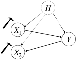
Figure 1: Graphical structure of an example of models (1) and (2). There is a hidden confounding variable $H$ and the hammers indicate that perturbations or interventions happen at the variables $X=(X_{1},X_{2})$ as in model (2).

2.2 Model for interventional distributions and heterogeneous data

In practical applications, interventions often happen to the system, leading to heterogeneity in the data. We consider here interventions on the covariates $X$. Our model for such interventional distributions is as follows. In model (1),

$$\begin{split}&\mbox{the random variable $X$ is replaced by the assigned new variable $X^{\mathrm{int}}=g(\varepsilon_{X})$, and}\\ &Y^{\mathrm{int}}\leftarrow f^{*}(X^{\mathrm{int}},\varepsilon_{Y}).\end{split}$$ (2)

Here, the function $g(.)$ could be random or deterministic and its argument is $\varepsilon_{X}=X$. This formulation encompasses various perturbation models. For example: if $g(\varepsilon_{X})\equiv x$ for a deterministic value $x$, this is a hard intervention and equals the do-operator $\mathrm{do}(X=x)$, as formally defined below. If $g(\varepsilon_{X})=\varepsilon_{X}+U$ for some random $U$, this is a shift intervention with random shift $U$. Thus, our perturbation model in (2) is rather general. We illustrate the models (1)-(2) in Figure 1.

Definition 1 (Do-interventional distribution).

In the perturbation model (2), let $X^{\mathrm{int}}=x$ for any $x\in\mathbb{R}^{d}$. We refer to the distribution of $Y^{\mathrm{int}}=f^{*}(x,\varepsilon_{Y})$ as the do-interventional distribution of $Y$ under $\mathrm{do}(X=x)$, denoted by $\pi^{*}_{y|x}$.

We remark that $\pi^{*}_{y|x}$ is the object we want to achieve, while the model in (2), which will be viewed later in (3) as the one for generating heterogeneous data, is more general than containing only do-interventions.

Consider now the setting where the data comes from different environments or sources $e=1,\ldots,E$ (Peters et al.,, 2016; Rothenhäusler et al.,, 2019; Arjovsky et al.,, 2019). We model the data as realizations for each environment $e$ as

$$X^{e}=g^{e}(\varepsilon_{X}),\ \ Y^{e}\leftarrow f^{*}(X^{e},\varepsilon_{Y}),\ e=1,\ldots,E.$$ (3)

Thus, the model for each environment in (3) is an intervention model as in (2), where each environment $e$ has its own perturbation or assignment function $g^{e}(.)$.

2.3 Proper scoring rules

To evaluate the accuracy of probabilistic predictions, we consider proper scoring rules. A proper scoring rule for a class of real-valued probability distributions $\mathcal{F}$ is a function $S:\mathcal{F}\times\mathbb{R}\to[-\infty,\infty]$ taking as arguments a probability distribution $F\in\mathcal{F}$ and an observation $Y\in\mathbb{R}$ satisfying

$$\mathbb{E}_{Y\sim F}[S(F,Y)]\leq\mathbb{E}_{Y\sim F}[S(G,Y)]$$ (4)

for all distributions $F,G\in\mathcal{F}$, where it is assumed that the expectations exist. A proper scoring rule $S$ is called strictly proper with respect to $\mathcal{F}$ if equality in equation (4) holds only if $F=G$. In Table 1, we give an overview of some commonly used proper scoring rules and we refer the interested reader to Gneiting and Raftery, (2007) for a general review. The two most popular proper scoring rules are the logarithmic score, which corresponds to negative log-likelihood, and the CRPS, which can be equivalently expressed as

$$\mathrm{CRPS}(F,Y)=\int_{-\infty}^{\infty}(1\{Y\leq z\}-F(z))^{2}\,dz.$$

Logarithmic score	Continuous ranked probability score	Scale invariant CRPS (Bolin and Wallin,, 2023)
LogS	CRPS	SCRPS
$-\log(g(Y))$	$\mathbb{E}_{\eta\sim G}|Y-\eta|-\mathbb{E}_{\eta,\eta^{\prime}\sim G}|\eta-\eta^{\prime}|/2$	$\mathbb{E}_{\eta\sim G}|Y-\eta|/\mathbb{E}_{\eta,\eta^{\prime}\sim G}|\eta-\eta^{\prime}|+\log(\mathbb{E}_{G}|\eta-\eta^{\prime}|)/2$
Pseudospherical score	Quadratic score	Hyvärinen score (Hyvärinen,, 2005)
PsueodoS	QS	HyvS
$-g(Y)^{\alpha-1}(\int_{-\infty}^{\infty}g(z)^{\alpha})\,dz)^{1/\alpha-1}$	$-2g(Y)+\int_{-\infty}^{\infty}g(z)^{2}\,dz$	$2g^{\prime\prime}(Y)/g(Y)-(g^{\prime}(Y)/g(Y))^{2}$

Table 1: Examples of strictly proper scoring rules for outcome $Y\in\mathbb{R}$ and a probability prediction $G$ with density $g$. In CRPS and SCRPS, the expectation is over independent $\eta,\eta^{\prime}$ with distribution $P$. For PseudoS, we have $\alpha>1$. See Gneiting and Raftery, (2007) for the scores without explicit reference.

Analogous to proper scoring rules for probabilistic predictions, Murphy and Daan, (1985) introduced the idea of consistent scoring functions for point predictions; see also Gneiting, (2011). For a real-valued univariate functional $T:\mathcal{F}\to\mathbb{R}$, a scoring function $L:\mathbb{R}\times\mathbb{R}\to[0,\infty)$ is consistent if

$$\mathbb{E}_{Y\sim F}[L(T(F),Y)]\leq\mathbb{E}_{Y\sim F}[L(t,Y)]$$

for all $t\in\mathbb{R}$ and $F\in\mathcal{F}$; if equality holds in the above display only if $t=T(F)$, then $L$ is a strictly consistent scoring function. As an example, the usual squared error loss $L(t,Y)=(t-Y)^{2}$ is a strictly consistent scoring function with respect to all distributions with finite second moment. By Theorem 3 of Gneiting, (2011), if $L$ is a consistent scoring function for $T$, then $S(F,Y):=L(T(F),Y)$ is a proper scoring rule, though not necessarily strictly proper.

In the standard definitions of both proper scoring rules and consistent scoring functions, the prediction is fixed. Typically, a prediction for an outcome variable $Y$ depends on observed covariates $X$, and in this case, the distributions and expected values in the definitions are to be understood conditional on $X$. We write $\pi_{y|x}$ to denote a probabilistic prediction for $Y$ given $X=x$. Formally, $\pi_{y|.}$ is a Markov kernel, meaning that $\pi_{y|x}$ is a probability distribution for each fixed $x\in\mathbb{R}^{d}$, and $x\mapsto\pi_{y|x}(A)$ is measurable for each Borel set $A\subseteq\mathbb{R}$. The subscript $y$ in $\pi_{y|x}$ is only notation to highlight that $\pi_{y|x}$ is a prediction for the response variable given $x$, and it has no mathematical implications; also, $\pi_{y|x}$ is generally not the (observational) conditional distribution of $Y$ given $X=x$. We define the risk of a prediction with respect to a proper scoring rule as

$$\mathcal{R}(\pi_{y|.},P,S)=\mathbb{E}_{(X,Y)\sim P}[S(\pi_{y|X},Y)].$$

3 Invariance and robustness in location-scale models

3.1 Impossibility of invariance under arbitrary interventions

In this section, we investigate invariance and robustness for location-scale models, specializing model (1) to

$$X=\varepsilon_{X},\quad Y\leftarrow\mu^{*}(X)+\sigma^{*}(X)\varepsilon_{Y},$$ (5)

where $\mu^{*}\colon\mathbb{R}^{d}\rightarrow\mathbb{R}$ and $\sigma^{*}\colon\mathbb{R}^{d}\rightarrow(0,1)$ are the location and scale functions respectively, and $\varepsilon_{Y}$ may be dependent of $X=\varepsilon_{X}$ as in model (1) due to hidden confounding. To motivate our definitions and results for probabilistic predictions, we first review the well-known robustness properties of the function $\mu^{*}(.)$ in point prediction without heteroscedasticy; that is, in the special case where $\sigma^{*}(X)\equiv 1$. More formally, a point prediction $\tilde{\mu}$ is invariant with respect to a class of distributions $\mathcal{P}$ and a loss function $L$ if, for all $P,P^{\prime}\in\mathcal{P}$,

$$\mathbb{E}_{P}[L(\tilde{\mu}(X),Y)]=\mathbb{E}_{P^{\prime}}[L(\tilde{\mu}(X),Y)].$$ (6)

Similarly, an invariant point prediction $\tilde{\mu}$ is robust if

$$\mathbb{E}_{P}[L(\tilde{\mu}(X),Y)]=\inf_{\mu}\sup_{P\in\mathcal{P}}\mathbb{E}_{P}[L({\mu}(X),Y)]$$ (7)

where the infimum is over all measureable functions $\mu:\mathbb{R}^{d}\to\mathbb{R}$. Results for point prediction are commonly formulated for mean prediction with squared error loss but, as discussed in Christiansen et al., (2022), there is an interest to study robustness for other loss functions. To this end, the following proposition provides such an extension.

Proposition 1.

Consider the additive noise model

$$X=\varepsilon_{X},\quad Y\leftarrow\mu^{*}(X)+\varepsilon_{Y},$$ (8)

as a special case of the model in (5). Let $T$ be a functional for which $T(\mathcal{L}(\varepsilon_{Y}))=0$, and let $L(t,Y)$ be a strictly consistent scoring function for $T$ that depends on $t$ and $Y$ only through $Y-t$ and for which $\mathbb{E}[L(0,\varepsilon_{Y})]$ exists. Let $\mathcal{P}$ be the set of all interventional distributions of $(X,Y)$ under the model given in (8). Then, $\mu^{\ast}(.)$ is the unique function satisfying (6) and (7).

An example where the above proposition extends mean prediction with the squared error loss is quantile prediction. If the $\alpha$-quantile of $\varepsilon_{Y}$ is unique and equal to zero, then $\mu^{*}(.)$ gives a worst-case optimal prediction for the $\alpha$-quantile under the loss quantile loss $L(t,Y)=(1\{t-Y\geq 0\}-\alpha)(t-Y)$. Interestingly, as shown by Gneiting, (2011), to achieve robustness in mean prediction without further assumptions, we must use the squared error loss function as it is the only consistent scoring function for the mean that depends on $t$ and $Y$ merely through $Y-t$.

We now generalize the ideas of invariance and robustness from point prediction to probabilistic prediction, which we define for the general model given in (1).

Definition 2 (Invariance).

A probabilistic prediction $\pi_{y|.}$ is said to be invariant with respect to a strictly proper scoring rule $S$ and a class of distributions $\mathcal{P}$ if there exists a constant $c\in\mathbb{R}$ such that

$$\mathcal{R}(\pi_{y|.},P,S)\equiv c,\ P\in\mathcal{P}.$$

For convenience, we refer to such predictions as $(S,\mathcal{P})$- invariant. If $\pi_{y|.}$ is $(S,\mathcal{P})$-invariant, then we may assume without any loss of generality that $c=0$ since $\tilde{S}(P,Y)=S(P,Y)-c$ is an equivalent proper scoring rule under which $\pi_{y|.}$ is $(\tilde{S},\mathcal{P})$-invariant with constant $c=0$.

Definition 3 (Robustness).

A probabilistic prediction $\pi_{y|.}$ is said to be distributionally robust with respect to a strictly proper scoring rule $S$ and a class of distributions $\mathcal{P}$ if

$$\sup_{P\in\mathcal{P}}\mathcal{R}(\pi_{y|.},P,S)\leq\sup_{P\in\mathcal{P}}\mathcal{R}(\pi^{\prime}_{y|.},P,S)$$

for all probabilistic predictions $\pi^{\prime}_{y|.}$. We denote such predictions as $(S,\mathcal{P})$-robust.

For the location-scale model, we have $\pi_{y|x}^{\ast}=\mathcal{L}(\mu^{\ast}(x)+\sigma^{\ast}(x)\varepsilon_{Y})$ for any $x$; that is, $\{\pi_{y|x}^{\ast}\}$ are a location-scale family with baseline distribution $Q^{\ast}$. This is analogous to the setting of point prediction where the function $\mu^{\ast}(X)=T[\mathcal{L}(\mu^{\ast}(X)+\varepsilon_{Y})]$ under the do-intervention $\mathrm{do}(X=x)$. Then, by the same arguments as in Proposition 1, we have that invariance implies robustness in the case of probabilistic prediction, as shown in the following proposition.

Proposition 2.

Consider the general model given in (1) and let $S$ be a strictly proper scoring rule and $\mathcal{P}$ be the family of all interventional distributions. If $\pi_{y|.}^{\ast}$ is $(S,\mathcal{P})$-invariant, then $\pi_{y|.}^{\ast}$ is an $(S,\mathcal{P})$-robust prediction and the risk under the observational distribution $P^{o}$, $\mathcal{R}(\pi^{*}_{y|.},P^{o},S)$, is minimal among the risks of all invariant $(S,\mathcal{P})$-invariant predictions.

Compared to Proposition 1, which shows that there exists an invariant and robust prediction for suitable strictly consistent scoring functions, Proposition 2 only shows that if $\pi_{y|.}^{\ast}$ is invariant, then it is also robust. As the following theorem demonstrates, if the class of distributions $\mathcal{P}$ contains all interventional distributions, there in fact does not necessarily exist any invariant prediction.

Theorem 3.

Assume the model in (5) with

$${X=\begin{pmatrix}X_{1}\\ X_{2}\end{pmatrix}=\begin{pmatrix}\varepsilon_{X_{1}}\\ \varepsilon_{X_{2}}\end{pmatrix},\quad Y\leftarrow\mu^{\ast}(X_{1})+\sigma^{\ast}(X_{2})\varepsilon_{Y},}$$ (9)

and additionally

• $\varepsilon_{Y}\sim\mathcal{N}(0,1)$ marginally;

• the functions $\mu^{*}\colon\mathbb{R}\rightarrow\mathbb{R}$ and $\sigma^{*}\colon\mathbb{R}\rightarrow(0,\infty)$ are surjective; and

• $\mathcal{P}$ contains the interventional distributions for all interventions on $X$ with any assignment value $x\in\mathbb{R}^{2}$.

Then there exists no strictly proper scoring rule $S$ such that $\pi^{*}_{y|.}$ is $(S,\mathcal{P})$-invariant.

The model in (9) is a Gaussian location-scale model, which is a special case of the general model given in (1). Thus, Theorem 3 shows that invariance in the sense of Definition 2 is generally not possible when $\mathcal{P}$ is the class of all interventional distributions on $X$. Hence, to obtain invariance, we must restrict our attention to finer classes of interventional distributions. From a practical perspective, it often fits the real-world scenario better not to look for robustness against all interventions, since some may not be encountered and considering all of them may lead to overly conservative predictions.

3.2 Restricted interventions

Naturally, there always exists a class of interventional distributions for which the proper scoring rule admits an invariant prediction; for example, if we consider the class of all interventional distributions with $\sigma^{\ast}(X)=1$, then we return to the setting of Proposition 1. However, such an intervention class is not of particular interest. As a first step towards identifying suitable and potentially practical interventional distributions, we explicitly compute the risk based on all six proper scoring rules given in Table 1.

Lemma 4.

Let $Q^{o}$ be the marginal distribution of $\varepsilon_{Y}$. For the model given in (5), we have

$$\begin{array}[]{ll}\mathrm{CRPS}(\pi_{y|X}^{*},Y)=\sigma^{*}(X)\mathrm{CRPS}(Q^{o},\varepsilon_{Y}),&\mathrm{LogS}(\pi_{y|X}^{*},Y)=\mathrm{LogS}(Q^{o},\varepsilon_{Y})+\log(\sigma^{*}(X)),\\ \mathrm{SCRPS}(\pi^{*}_{y|X},Y)=\mathrm{SCRPS}(Q^{o},\varepsilon_{Y})+\log(\sigma^{*}(X))/2,&\mathrm{PseudoS}(\pi_{y|X}^{*},Y)=\sigma^{*}(X)^{1/\alpha-1}\mathrm{PseudoS}(Q^{o},\varepsilon_{Y}),\\ \mathrm{QS}(\pi_{y|X}^{*},Y)=\sigma^{*}(X)^{-1}\mathrm{QS}(Q^{o},\varepsilon_{Y}),&\mathrm{HyvS}(\pi_{y|X}^{*},Y)=\sigma^{*}(X)^{-2}\mathrm{HvyS}(Q^{o},\varepsilon_{Y}),\end{array}$$

where it is assumed that $Q^{o}$ admits a density with respect to Lebesgue measure for the cases of LogS, PseudoS, and QS, and that the density is twice differentiable for the case of HyvS.

The above result implies that, to formulate a restricted intervention class for invariant predictions under LogS and SCRPS, we only need knowledge of the marginal distribution of $X$. On the other hand, for CRPS, PseudoS, QS, and HyvS, knowledge of the joint distribution between $X$ and $\varepsilon_{Y}$ is generally required. In practice, the latter necessitates understanding of the underlying structural and confounding mechanism, which, in most applications, is not realistic. Meanwhile, for LogS and SCRPS, an invariant risk is equivalent to $\mathbb{E}_{P}[\log(\sigma^{*}(X))]$ being constant under interventional distributions $P$, which depends on the covariates and the interventions only and not on the confounding mechanism. This leads us to the following result.

Lemma 5 (Exponential scale parametrization).

For the location-scale model given in (5), assume that $\sigma^{*}(X)=\exp(\gamma^{\top}X)$ for some $\gamma\in\mathbb{R}^{d}$. Then, LogS and SCRPS proper scoring rules admit an invariant prediction with respect to the class of interventional distributions $P$, generated as in (2), for which

$$\mathbb{E}_{P}[X]-\mathbb{E}_{P^{o}}[X]\perp\gamma.$$

For heteroscedastic linear models, the exponential scale $\sigma^{\ast}(X)$ is a popular assumed parametric form for the variance term that, to the best of our knowledge, was first considered by Cook and Weisberg, (1983). For general location-scale models with linear scale parametrization and exponential link, interventions under which the expectation of $X$ remains constant or is shifted in a direction orthogonal to $\gamma$ do not affect the risk with respect to LogS and SCRPS. Clearly, $\pi^{*}_{y|.}$ is not the unique $(S,\mathcal{P})$-invariant probabilistic prediction under the distributions in Lemma 5. If $\pi^{\prime}_{y|x}=\mathcal{L}(\mu^{*}(x)+\sigma^{*}(x)\eta)$ and $\eta$ follows an arbitrary distribution $Q^{\prime}$, then $S(\pi^{\prime}_{y|X},Y)=S(\pi^{*}_{y|X},Y)$ with LogS or SCRPS. But since $\mathrm{LogS}(Q^{\prime},\varepsilon_{Y})>\mathrm{LogS}(Q^{o},\varepsilon_{Y})$, and analogously for the SCRPS, the prediction $\pi^{*}_{y|.}$ achieves a smaller risk than location-scale families with a misspecified baseline distribution. However, in general it is not obvious whether there exist other predictions with misspecified location or scale functions that achieve a smaller, invariant risk than $\pi^{*}_{y|.}$, since our setting generally does not allow do-interventions and Proposition 2 does not apply. The following example shows that in the Gaussian heteroscedastic linear regression model with LogS, one can indeed identify $\pi^{*}_{y|.}$ as the unique prediction method with a minimal invariant risk.

Example 1.

Assume that $(\varepsilon_{Y},\varepsilon_{X}^{\top})^{\top}$ are Gaussian with mean $0$ and covariance matrix $\Sigma\in\mathbb{R}^{(d+1)\times(d+1)}$ with $\Sigma_{11}=1$. Let $\mu^{*}(x)=\beta^{\top}x$ and $\sigma^{*}(X)=\exp(\gamma^{\top}x)$, and let

$$\pi_{y|x}=\mathcal{N}(b^{\top}x,\exp(2g^{\top}x))$$

for some $b,g\in\mathbb{R}^{d}$. We consider finitely many interventions on the covariance structure of $X$ to formulate identifiability conditions; more precisely, we assume

$$X^{e}=\Gamma^{e}\varepsilon_{X},\quad Y^{e}\leftarrow\beta^{\top}X^{e}+\exp(\gamma^{\top}X^{e})\varepsilon_{Y},$$

where $e=1,\dots,E$ are the observations under $E$ different environments as in model (3), with different interventions that are multiplication of $\varepsilon_{X}$ with some invertible matrix $\Gamma^{e}$. Then,

$$2\,\mathrm{LogS}(P_{y\mid X^{e}},Y^{e}) =\left(\varepsilon_{Y}\exp((\gamma-g)^{\top}\Gamma^{e}\varepsilon_{X}))+(\beta-b)^{\top}\Gamma^{e}\varepsilon_{X}\exp(-g^{\top}\Gamma^{e}\varepsilon_{X})\right)^{2}+g^{\top}\Gamma^{e}\varepsilon_{X}+c,$$

where $c$ is a constant not depending on the parameters. Let $\Sigma_{X}=(\Sigma_{ij})_{i,j=2}^{d+1}$ be the covariance matrix of $\varepsilon_{X}$ and $\Sigma_{YX}=(\Sigma_{i1})_{i=2}^{d+1}$ the covariance between $\varepsilon_{X}$ and $\varepsilon_{Y}$. Since the mean of $\varepsilon_{X}$ is zero, we have $\mathbb{E}[g^{\top}\Gamma^{e}\varepsilon_{X}]=0$, and the expected logarithmic score equals

$$2\,\mathbb{E}[\mathrm{LogS}(P_{y\mid X^{e}},Y^{e})] =\left((\beta-b)^{\top}\Gamma^{e}\Sigma_{X}(\Gamma^{e})^{\top}(\beta-b)+4((\beta-b)^{\top}\Gamma^{e}\Sigma_{X}(\Gamma^{e})^{\top}g)^{2}\right)\exp(2g^{\top}\Gamma^{e}\Sigma_{X}(\Gamma^{e})^{\top}g)$$

$$\quad+\exp(2(\gamma-g)^{\top}\Gamma^{e}\Sigma_{X}(\Gamma^{e})^{\top}(\gamma-g))$$

$$\quad+2(\beta-b)^{\top}\Gamma^{e}\Sigma_{YX}\exp((\gamma-2g)^{\top}\Gamma^{e}\Sigma_{X}(\Gamma^{e})^{\top}(\gamma-2g)/2)+c.$$

From the above calculations, we see that one of the following are sufficient conditions for $\beta$ and $\gamma$ to be uniquely identified as the parameters attaining the minimal invariant risk.

Scenario 1.

If there is no confounding, meaning that $\Sigma_{YX}=0$, then the minimal risk is always achieved uniquely by $b=\beta$ and $g=\gamma$. This follows from the formula above, where the third term vanishes, or directly from strict propriety of the logarithmic score, and invariance holds because $\Gamma^{e}X$ has mean zero for all $e$.

Scenario 2.

If $b=\beta$, or if there is no location parameter ($\beta=b=0$), then only $g=\gamma$ achieves a minimal constant risk if there are two environments for which $\Gamma^{e}\Sigma_{X}(\Gamma^{e})^{\top}\prec\Gamma^{e^{\prime}}\Sigma_{X}(\Gamma_{e^{\prime}})^{\top}$, i.e. $\Gamma^{e^{\prime}}\Sigma_{X}(\Gamma^{e^{\prime}})^{\top}-\Gamma^{e}\Sigma_{X}(\Gamma^{e})^{\top}$ is strictly positive definite.

Scenario 3.

Assume that $E\geq d+1$ and there exist $d$ environments $e_{1},\dots,e_{d}$ such that $\Gamma^{e_{j}}\Sigma_{YX}$, $j=1,\dots,d$, are linearly independent, and an environment $e_{d+1}$ such that $\Gamma^{e_{d+1}}\Sigma_{YX}=\sum_{j=1}^{d}\alpha_{j}\Gamma^{e_{j}}\Sigma_{YX}$ for some $\alpha_{j}\leq 0$, $j=1,\dots,d$. Then the risk is constant and minimal only if $b=\beta$ and $g=\gamma$.

Scenario 1 reiterates the general fact that $\pi_{y|.}^{*}$ is optimal if there is no confounding. A weakened condition appears in Christiansen et al., (2022) as the existence of a “confounding removing intervention”, which means that $X^{e}$ and $Y^{e}$ are unconfounded in at least one environment $e$, and not necessarily in all environments. Typically this is only achieved with do-interventions, but as we have seen in Theorem 3, one usually cannot expect an invariant risk under such interventions. In a scale model, Scenario 2, we have identifiability under the condition of ordered variances, and a similar assumption is made in Shen et al., (2023). Scenario 3 assumes that there is sufficient variation in the confounding between $X$ and $Y$, and is a natural identifiability condition. In particiular, it only requires $d+1$ different interventions to identify the two $d$-dimensional location and scale parameters.

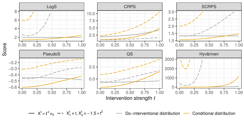
Figure 2: Scores for the illustrative example from Section 3.2, with $\alpha=2$ for PseudoS.

To help elucidate our theoretical results up to this point, we end this section with an illustrative example. Consider the model

$$\begin{pmatrix}\varepsilon_{Y}\\ \varepsilon_{X_{1}}\\ \varepsilon_{X_{2}}\end{pmatrix}\sim\mathcal{N}_{3}\left(0,\begin{pmatrix}3&1&1\\ 1&1&0\\ 1&0&1\\ \end{pmatrix}\right)\!,\quad X=\varepsilon_{X},\quad Y\leftarrow X_{1}+\exp(X_{2})\varepsilon_{Y}$$

with the test intervention classes $\{\mathrm{do}(X_{1}^{t}=t,X_{2}^{t}=-1.5+t^{2}):0\leq t\leq 1\}$ and

$$\{X^{t}=\Gamma^{t}\varepsilon_{X}:\Gamma^{t}=\begin{pmatrix}1&t\\ t&1\end{pmatrix},0\leq t\leq 1\}.$$

Here, $t$ measures the strength of the intervention. Figure 2 plots the scores of the do-interventional distribution $\pi^{*}_{y|.}$ and the conditional distribution $P^{o}_{y|.}$ as a function of the intervention strength $t$. From our results above, we know that the LogS and SCRPS of the prediction $\pi^{*}_{y|.}$ are constant under the intervention $X^{t}=\Gamma^{t}\varepsilon_{X}$ for all $t$. This is not true for the conditional distribution $P^{o}_{y|.}$ in the observational environment, which is only optimal for $t=0$ and exhibits deteriorating accuracy with respect to all scores. Under the do-intervention, the prediction $\pi^{*}_{y|.}$ is optimal, but not invariant with respect to any of the scores.

4 Invariant probabilistic prediction

The derivations and examples in the previous sections suggest that, in order to find an invariant and thus robust probabilistic prediction, one should seek for a $\pi_{y|.}$ that achieves a minimal, constant risk across different interventional distributions. In this section, we consider the model for multiple environments given in (3), with each environment $e=1,\dots,E$ corresponding to one distinct intervention.

Assume that the candidate predictions $\pi_{y|.}$ are parametrized by some $\theta\in\Theta\subset\mathbb{R}^{d}$, for which we write $\pi_{y|.,\theta}$. For example, in the exponential location-scale model from Lemma 5, we have $\theta=(\beta^{\top},\gamma^{\top})^{\top}$. Let $S$ be a strictly proper scoring rule and define the empirical risk and its expectation in environment $e$ by

$$\hat{\mathcal{R}}^{e}(\theta)=\frac{1}{n_{e}}\sum_{i=1}^{n_{e}}S(\pi_{y|X^{e}_{i},\theta},Y^{e}_{i}),\quad\mathcal{R}^{e}(\theta)=\mathbb{E}[\hat{\mathcal{R}}^{e}]=\mathcal{R}(\pi_{y|.,\theta},P^{e},S),$$

where $(X^{e}_{i},Y^{e}_{i})$, $i=1,\dots,n_{e}$, are independent and identically distributed observations in environment $e$. It is always assumed that the expectations above are finite. Now, we can define our proposed estimator, invariant probabilistic prediction.

Definition 4 (Invariant probabilistic prediction (IPP)).

Let $S=S(P,Y)$ be a strictly proper scoring rule, $D\colon\mathbb{R}^{E}\rightarrow[0,\infty)$ be continuous a function such that $D(v)=0$ if and only if $v_{1}=\dots=v_{k}$, $\lambda\geq 0$ be a tuning parameter, and $\{\omega^{e}\}_{e=1}^{E}$ be convex weights.

The invariant probabilistic prediction is defined as $P_{y|x,\hat{\theta}(\lambda)}$, where $\hat{\theta}(\lambda)$ is a minimizer of

$$\hat{R}_{\lambda}(\theta)=\sum_{e=1}^{E}\omega^{e}\hat{\mathcal{R}}^{e}(\theta)+\lambda D(\hat{\mathcal{R}}^{1}(\theta),\dots,\hat{\mathcal{R}}^{E}(\theta)),$$ (10)

if it exists.

We describe our preferred choices for $\{\omega^{e}\}_{e=1}^{E}$ and $D$ at the end of the section. Our proposed IPP estimator turns out to be a generalization of the V-REx estimator of Krueger et al., (2021), who consider the special case where the convex weights are uniform and the regularization function is the variance,

$$D(v)=\frac{1}{E^{2}}\sum_{1\leq i<j\leq E}(v_{i}-v_{j})^{2}.$$ (11)

However, IPP is derived in a much more formal and general manner by characterizing the invariance of probabilistic prediction, and its theoretical properties are well demonstrated. In particular, the following theorem shows that, under mild regularity conditions, IPP yields a consistent estimator of the underlying parameter and an invariant prediction.

Theorem 6.

Consider the model given in (3). Suppose

1. there exists a unique $\theta^{\ast}\in\Theta$ such that $\mathcal{R}^{1}(\theta^{*})=\dots=\mathcal{R}^{E}(\theta^{*})$ and $\mathcal{R}^{1}(\theta^{*})$ is minimal among the parameters achieving an invariant risk;

2. the number of observations in each environment satisfies $n:=\min(n_{1},\dots,n_{E})\to\infty$;

3. the parameter space $\Theta$ is compact;

4. the function $S(\pi_{y|x,\theta},y)$ is continuous in $\theta$ for all $(x,y)$;

5. there exists $0<B<\infty$ such that $\mathbb{E}[\sup_{\theta\in\Theta}S(P_{y|X^{e},\theta},Y^{e})^{2}]\leq B$, $e=1,\dots,E$;

6. the sequence $\lambda_{n}\to\infty$ and the regularization function $D$ satisfy

   $$\sup_{\theta\in\Theta}\lambda_{n}|D(\hat{\mathcal{R}}^{1}(\theta),\dots,\hat{\mathcal{R}}^{E}(\theta))-D(\mathcal{R}^{1}(\theta),\dots,\mathcal{R}^{E}(\theta))|=o_{P}(1),$$

then $\hat{\theta}(\lambda_{n})$ is consistent for $\theta^{\ast}$. If, in addition,

1. the family $\{\pi_{y|x,\theta}\}$ is continuous in $\theta$ for a fixed $x$,

then $\pi_{y|x,\hat{\theta}(\lambda)}$ is consistent for $\pi_{y|x,\theta^{\ast}}$.

The first assumption ensures that the invariant population parameter $\theta^{\ast}$ is identified and, effectively, imposes a restriction on the class of interventions. As demonstrated in Example 1, this assumption is satisfied for the Gaussian heteroscedastic linear regression model with $\mathrm{LogS}$, while such a specific model is not required in our consistency result. Assumption 2 requires the number of observations in each environment to diverge, to ensure sufficient information about all of the environments. Assumptions 3, 4, 5, and 7 are standard conditions for consistency. For instance, Assumptions 4 and 5 are satisfied in Example 1 if the parameter space is compact.

The remaining Assumption 6 concerns the penalty. In particular, the exact choice of $\lambda_{n}$ depends on the regularization function $D$. The following corollary gives an explicit characterization of this assumption in the setting where $D$ is the variance function in (11).

Corollary 7.

Consider the model given in (1). Suppose Assumptions 1 – 5 and 7 hold. If $D$ is the variance function given in (11) and $\lambda_{n}\to\infty$ with $\lambda_{n}=O(n^{1/2}\log(n)^{-1/2})$, then Assumption 6 is satisfied. Moreover, the conclusions of Theorem 6 hold.

Theorem 6 only gives an upper bound on the rate at which $\lambda$ may diverge, but it does not give guidance of how to choose $\lambda$ in applications. Our strategy, which is inspired by Jakobsen and Peters, (2021) and yields good results in our experiments, is to select a minimal $\lambda$ for which there are no significant differences between the environment risks. More precisely, let $\hat{T}(\theta)$ be a test statistic depending on $\theta$ and $(X_{i}^{e},Y_{i}^{e})$, $i=1,\dots,n_{e}$, $e=1,\dots,E$, such that higher values of $\hat{T}(\theta)$ indicate a violation of the hypothesis $\mathcal{R}^{1}(\theta)=\dots=\mathcal{R}^{E}(\theta)$. Assume that the (asymptotic) distribution function $F$ of $\hat{T}(\theta)$ in the case that $\mathcal{R}^{1}(\theta)=\dots=\mathcal{R}^{E}(\theta)$ is known. Then for $\alpha\in(0,1)$,

$$C(\alpha)=\{\theta\in\Theta\colon F(\hat{T}(\theta))\leq 1-\alpha\}$$

is an (asymptotic) confidence set for the parameter $\theta^{*}$. We then choose the parameter $\lambda$ as

$$\hat{\lambda}=\inf\{\lambda\geq 0\colon\hat{\theta}(\lambda)\in C(\alpha)\},$$

i.e. we increase the penalty $\lambda$ until the sample estimator $\hat{\theta}_{\lambda}$ lies in the confidence set $C(\alpha)$. Hence the choice of $\lambda$ is reduced to finding the minimal penalty parameter for which the null hypothesis of equal risks is not rejected, for a small confidence level $\alpha$. Notice that there is no guarantee that the p-value $F(\hat{T}(\hat{\theta}_{\lambda}))$ is increasing in $\lambda$, but in practice one observes this in most cases due to the following simple result.

Lemma 8.

The function $\lambda\mapsto D(\hat{\mathcal{R}}^{1}(\theta(\lambda)),\dots,\hat{\mathcal{R}}^{E}(\theta(\lambda)))$ is non-increasing in $\lambda$, and $\lambda\mapsto\sum_{e=1}^{E}\hat{\mathcal{R}}^{e}(\theta(\lambda))$ is non-decreasing in $\lambda$.

In our empirical applications, we use the generalization of Welch’s two sample t-test with unequal variances implemented in the function oneway.test in R. The weights in Definition 4 are taken as $\omega^{e}=1/E$, $e=1,\dots,E$, and for the function $D$, we choose the variance (11) for computational simplicity.

5 Empirical results

5.1 Simulations

We illustrate IPP in the setting of Example 1. For $d=5$, we generate $(\varepsilon_{Y},\varepsilon_{X})\sim\mathcal{N}_{d+1}(0,\Sigma)$, where

$$\Sigma_{ii}=1,i=1,\dots,d+1,\ \Sigma_{12}=0.8,\ \Sigma_{13}=-0.4,\ \Sigma_{14}=0.3,\ \Sigma_{15}=-0.2,\ \Sigma_{16}=0.1,$$

and $\Sigma_{ij}=0$ for all other $i,j$. That is, $\varepsilon_{X}$ has independent standard normal entries, but there is confounding, due to the non-zero correlations with $\varepsilon_{Y}$. In environments $e=1,\dots,d$, we define

$$X^{e}=\Gamma^{e}\varepsilon_{X},\,(\Gamma^{e})_{ij}=1\{i=j\}+U_{ij},\,U_{ij}\sim\mathrm{Unif}(-0.1,0.1),$$

$$\beta=(\beta_{1},\dots,\beta_{d}),\,\beta_{j}\sim\mathrm{Unif}(0,3),\quad\gamma=(\gamma_{1},\dots,\gamma_{d}),\,\gamma_{j}\sim\mathrm{Unif}(0,0.5),\ j=1,\dots,d,$$

$$Y^{e}=\sum_{j=1}^{d}X_{j}^{e}\beta_{j}+\exp\Big{(}\sum_{j=1}^{d}\gamma_{j}X_{j}^{e}\Big{)}\varepsilon_{Y},$$

where all the random parameters are chosen independently. With this construction, the covariance of $X$ is slightly different in each environment but close to the identity matrix. For environment $d+1$ the data is generated in the same way, but $\Gamma^{d+1}=\sum_{e=1}^{d}\alpha^{e}\Gamma^{e}$ for random $\alpha^{e}\leq 0$ summing to $-1$. Condition 3 in Example 1 is satisfied with probability one in this simulation study. We consider $\lambda\in\{0,0.5,1,\dots,15\}$ and sample sizes of $n^{e}=100,150,200,250,500,1000$ in each environment. Estimation is done with $S=\mathrm{LogS}$ and $S=\mathrm{CRPS}$, and the figures for the latter are given in Appendix C.

We implemented our methods in R and Python, and provide code and replication material for all our empirical results on https://github.com/AlexanderHenzi/IPP. Details about the computation of IPP are given in Appendix B.

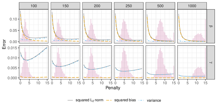
Figure 3: Simulation study: Estimation error for $\beta$ (top) and $\gamma$ (bottom) as a function of the penalty parameter, separated into squared bias and variance, for different values of $n^{e}$. The different sample sizes are given on top of each panel. The bars show height-adjusted frequencies with which each $\lambda$ is chosen by the rule described in Section 4 with $\alpha=0.05$, and $\lambda$ is set to the maximal value $15$ for this experiment if the hypothesis of equal risk is rejected for all $\lambda$.

Figure 3 shows the mean parameter estimation errors $\mathbb{E}[\|\hat{\beta}_{\lambda}-\beta\|^{2}]$ and $\mathbb{E}[\|\hat{\gamma}_{\lambda}-\gamma\|^{2}]$, and their decomposition into bias and variance. For the location parameter, regression without penalization is biased, and as $\lambda$ increases, the bias decreases. For the scale parameter the bias is negligible but the variance decreases for moderate $\lambda$. Choosing $\lambda$ too large deteriorates the estimator for both location and scale parameter. Our heuristic rule for choosing the $\lambda$ with $\alpha=0.05$ often selects a penalty parameter that gives small estimation errors. Levels of $\alpha=0.01$ or $\alpha=0.1$ yield slightly smaller or greater $\lambda$, respectively, but qualitatively the same results; see Figures 9 and 10 in Appendix C.

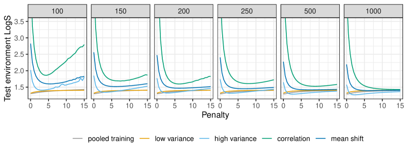
Figure 4: Simuation study: Mean logarithmic score on new test environment arising from different interventions as described in the text.

In Figure 4 we depict the mean logarithmic score when predicting on test environments. If the data in the test environment has the same distribution as the pooled training data, then distributional regression without penalitation is clearly the best choice. We then tested variance interventions, where $X^{e}=c^{e}\varepsilon_{X}$ for $c^{e}=1/3,\,3/2$, which are labelled as low and high variance interventions, respectively. Furthermore, we applied an intervention on the correlation structure, where

$$X^{e}=\Gamma^{e}\varepsilon_{X},\ \Gamma_{ij}^{e}\sim 1\{i=j\}+\mathrm{Unif}(-0.75,0.75),\ i,j=1,\dots,d,$$

and a mean shift intervention orthogonal to $\gamma$,

$$X^{e}=\varepsilon_{X}+\delta^{e}-\gamma((\delta^{e})^{\top}\gamma)/\|\gamma\|^{2},\ \delta^{e}_{j}\sim\mathrm{Unif}(-5,5),\ j=0,\dots,d.$$

While IPP is not guaranteed to have a minimal error under all interventions, we observe that it does minimize the maximum error among the classes of interventions considered, in comparison to distributional regression without penalization. Also, it can be seen that the error under interventions for large $\lambda$ is almost constant across different interventions, at least for sufficiently large sample sizes, which is not the case for distributional regression.

We refrain from comparing IPP to other methods in the simulation study, as all the methods known to us operate under different conditions and it seems impossible to find a setting where none of them is misspecified, apart from trivial location models with homoscedastic error. Instead, we make such comparisons through real data.

5.2 Application on single-cell data

So far we have demonstrated that IPP achieves, under ideal conditions, an invariant risk under certain classes of interventions on the covariates. In practice, one would hope that even in a misspecified setting or when interventions do not only act on the covariates, equalizing training risks still has a positive effect on the out-of-distribution performance in new environments. We investigate this in an application on single-cell data, similar to Shen et al., (2023, Section 6). Our data consists of measurements of the expression of 10 genes, one of which is chosen as the response variable and the others as covariates. The training data comprises 9 environments, where each of the covariate genes is intervened on with CRISPR pertubations, and an additional observational environment without interventions. The number of observations range from $101$ to $552$ for the interventional environments with the perturbed genes, and equals $11485$ for the observational environment. In addition to the training data, observations from more than $400$ environments with interventions on other genes are available. We evaluate predictions on the 50 environments in which the distribution of the 10 observed genes has the largest energy distance (Székely et al.,, 2004) from their distribution in the pooled training data.

We first apply IPP with the heteroscedastic Gaussian linear model,

$$\pi_{y|x}=\mathcal{N}(\beta_{0}+\beta^{\top}x,\,\exp(2\gamma_{0}+2\gamma^{\top}x)),$$

where $x$ is the vector of expressions of the $9$ covariate genes, and perform estimation with LogS and SCRPS as loss functions. Figure 5 illustrates the training risks of above versions of IPP as a function of the penalty parameter, and the corresponding p-values for testing equality of training risks. For the LogS, a significance level of $\alpha$ between $0.05$ and $0.1$ would select a penalty parameter between $20$ and $30$. For the SCRPS a value of about $50$ is required to achieve non-significant difference between training risks.

As an extension, we apply IPP with the model (1) in full generality. Specifically, we adopt a model $Y=f_{\theta}(X,\varepsilon)$ with a nonlinear function $f_{\theta}(X,\varepsilon)$ parametrized by neural networks, taking as arguments the covariates $X$ and multivariate Gaussian $\varepsilon$ representing the noise. A probabilistic prediction $\pi_{y|x}$ is obtained by resampling the noise $\varepsilon$ while fixing $X=x$. Such general parametrizations of probabilistic predictions have been used in the literature (Shen and Meinshausen,, 2023), and due to the flexibility of the function class for $f_{\theta}$, the choice of the distribution of $\varepsilon$, here specified as Gaussian, usually has no impact on the outcome distribution. In this general setting, the conditional distribution does not have a closed-form density so we cannot evaluate the LogS explicitly, but the generative nature of this model enables estimation of the SCRPS by sampling. Thus, we apply IPP with the SCRPS as the loss function, and refer to this as a neural network implementation (NN) of IPP with SCRPS. The details of hyperparameters for model training are given in Appendix B.

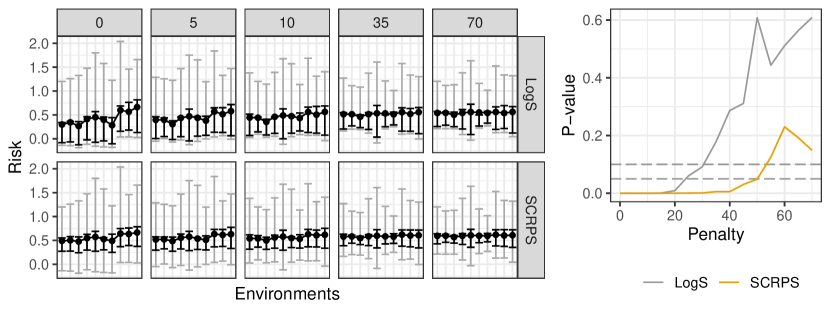
Figure 5: Single cell data: Training risks of IPP over different environments (left panel). The first environment is the observational environment, and the panel columns are different penalty parameter values. The right panel shows the p-value of the oneway.test for equal training risks as a function of the penalty. Horizontal lines indicate the levels of $0.05$ and $0.1$.

As a competitor for probabilistic prediction, we apply distributional anchor regression (Kook et al.,, 2022) with $F_{y|x}(z)=\Phi(h(z)-\beta^{\top}x)$ for a strictly increasing function $h$ parametrized with Bernstein polynomials and estimated jointly with $\beta$. Due to optimization problems with large data sets, we had to exclude the observational environment for this method, and to ensure a fair comparison, Appendix C includes a figure of the prediction error when IPP is also applied without the observational environment, where the advantage over distributional anchor regression remains similar.

In addition to the distributional methods, we reduce the probabilistic predictions to their conditional means and compare with respect to the mean squared error (MSE) against methods aimed for mean prediction, such as anchor regression (Rothenhäusler et al.,, 2021) and DRIG (Shen et al.,, 2023). The setting for distributional anchor regression, anchor regression, and DRIG does allow interventions on the response variable, and we investigate the influence of including the corresponding environment in the training data in Appendix C. Finally, as another baseline method for point prediction, we test V-REx (Krueger et al.,, 2021) with $y=f_{\theta}(x)$ parametrized by neural networks with the same architecture as our NN implementation of IPP. In this method, the loss function is of the same form as in IPP but with the MSE as risk, i.e., $\mathcal{R}^{e}(\theta)=\mathbb{E}[(Y^{e}-f_{\theta}(X^{e}))^{2}]$.

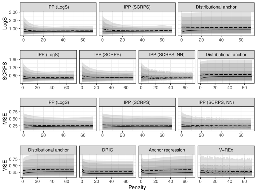
Figure 6: Single cell data: Errors on the $50$ test environments for the different methods. The solid and dashed line show the median and mean environment prediction error, and the shaded bands are delimited by the $j/10$- and $(10-j)/10$-quantiles, $j=0,\dots,4$ of the mean prediction errors over the $50$ environments, respectively.

Figure 6 depicts the prediction errors on test data, including LogS and SCRPS for distributional methods to evaluate the probabilistic prediction performance, and MSE for all methods to evaluate the mean prediction. IPP always stands as the most competitive method regardless of the loss function and model class used, as it consistently achieves the smallest prediction errors, especially the worst-case error, and also the smallest variation in the prediction errors across all test environments. It exhibits similar advantages even in terms of point prediction for the mean over the methods designed for mean prediction. Interestingly, when heteroscedastic Gaussian linear models are used, estimating IPP with the logarithmic score as the loss function outperforms the estimation with SCRPS, even when evaluated with respect to the latter score, suggesting that a more classical approach with log-likelihood as loss function fits the model better.

A suitable penalization strength generally improves all methods. The penalty parameters selected for IPP in the heteroscadastic Gaussian linear version, based on the p-values in Fig. 5, yield a stable and small error both under LogS and SCRPS, showing the usefulness of our scheme for selecting the penalty. The effect of penalty tuning is the weakest for distributional anchor regression, where a small but positive penalty parameter improves the test errors only slightly.

With the general model class using neural network parametrization, IPP exhibits slightly better performance compared to the heteroscedastic Gaussian linear model, especially with a larger penalty parameter. The performance across different test environments also tends to be less variable, indicated by the smaller spreads. Notably, this improvement does not come only from the flexibility of the model class. In fact, the V-REx method, which is also based on neural networks, is inferior to the NN variant of IPP in terms of both the average risk and variability, in spite of the fact that it is optimized to have small and constant risks in terms of MSE on training data. This highlights that even if one is interested in point prediction, it may be beneficial to apply distributional methods and then deduce any summary statistic such as the mean or the median.

6 Discussion

We considered and analyzed invariance for probabilistic predictions under structural equation models, aka a causality-inspired framework (Peters et al.,, 2016; Rojas-Carulla et al.,, 2018; Bühlmann,, 2020). In contrast to point estimation, which has been studied in a lot of recent works, the rigorous formulation for probabilistic predictions has not been worked in detail. We described the fundamental difficulties and brought up a constructive algorithm, called Invariant Probabilistic Prediction (IPP), which is shown to have desirable theoretical properties, as well as exhibiting good and robust performance on simulated and real data. We believe that our fundamental formulation would lead to some avenues of future research in various directions, including more detailed robustness against a finite amount of distribution shifts, instead of full invariance, or rigorous analysis of invariance and identifiability in more complex nonlinear models.

Appendix A Proofs

A.1 Proof of Proposition 1

Proof.

The first equality holds because the distribution of $L(\mu^{*}(X),Y)$ only depends on $\varepsilon_{Y}$, which is invariant under interventions on $X$. For the second equality, notice that for any $\mu$,

$$\sup_{P\in\mathcal{P}}\mathbb{E}_{P}[L(\mu(X),Y)]\geq\mathbb{E}_{\mathrm{do}(X=x)}[L(\mu(x),Y)]\geq\mathbb{E}_{\mathrm{do}(X=x)}[L(\mu^{*}(X),Y)]=\mathbb{E}[L(\mu^{*}(X),Y)].$$

Here $x\in\mathbb{R}$ is arbitrary, and the second inequality holds because $L(\mu^{*}(x),Y)=L(0,\varepsilon_{Y})$ and because $0=T(\mathcal{L}(\varepsilon_{Y}))$; equality holds if and only if $\mu(x)=\mu^{*}(x)$ due to strict consistency of $L$. ∎

A.2 Proof of Theorem 3

Proof.

To obtain a contradiction, suppose that there exists a strictly proper scoring rule $S$ such that $\pi^{*}_{y|.}$ is $(S,\mathcal{P})$-invariant, which we assume without any loss of generality that $c=0$. We have

$$0=\mathbb{E}_{\mathrm{do}(X=(x_{1},x_{2}))}[S(\mathcal{N}(\mu^{*}(X_{1}),\sigma^{*}(X_{2})^{2}),Y)]=\mathbb{E}_{Y\sim\mathcal{N}(\mu^{*}(x_{1}),\sigma^{*}(x_{2})^{2})}[S(\mathcal{N}(\mu^{*}(x_{1}),\sigma^{*}(x_{2})^{2}),Y)].$$

Since $\mu^{*}$ and $\sigma^{*}$ are surjective, this yields

$$0=\mathbb{E}_{Y\sim\mathcal{N}(\mu,\sigma^{2})}[S(\mathcal{N}(\mu,\sigma^{2}),Y)]$$

for all fixed $\mu\in\mathbb{R}$, $\sigma>0$. Because $S$ is strictly proper, we also know

$$\mathbb{E}_{Y\sim\mathcal{N}(m,s^{2})}[S(\mathcal{N}(m,s^{2}),Y)]=0<\mathbb{E}_{Y\sim\mathcal{N}(m,s^{2})}[S(\mathcal{N}(\mu,\sigma^{2}),Y)]$$ (12)

for all $m\in\mathbb{R}$ and $s>0$ such that $m\neq\mu$ or $s\neq\sigma$. Let $V=Z+Z^{\prime}$, where $Z,Z^{\prime}\sim\mathcal{N}(0,1)$ independent, so $V\sim\mathcal{N}(0,2)$. Then we have

$$\mathbb{E}[S(\mathcal{N}(0,2),V)]=\mathbb{E}[\mathbb{E}[S(\mathcal{N}(0,2),Z+Z^{\prime})\mid Z]]>0,$$

because $\mathbb{E}[S(\mathcal{N}(0,2),Z+Z^{\prime})\mid Z]>0$ a.s. by (12), since $Z+Z^{\prime}\sim\mathcal{N}(Z,1)$ conditional on $Z$. This contradicts $\mathbb{E}[S(\mathcal{N}(0,2),V)]=0$. ∎

A.3 Proofs for Example 1

The following lemma is applied several times in the proof.

Lemma 9.

If $X\sim\mathcal{N}_{n}(0,\Sigma)$ and $\theta\in\mathbb{R}^{n}$, then

$$\mathbb{E}[h(X)\exp(\theta^{\top}X)]=\mathbb{E}[h(Y)]\exp(\theta^{\top}\Sigma\theta/2),$$

where $h\colon\mathbb{R}^{n}\rightarrow\mathbb{R}$ is any function such that the expected value exists, and $Y\sim\mathcal{N}(\Sigma\theta,\Sigma)$.

Proof of Lemma 9.

Combining the factor $\exp(\theta^{\top}X)$ with the multivariate Gaussian density gives

$$h(x)c(\Sigma)\exp(\theta^{\top}x)\exp(-x^{\top}\Sigma^{-1}x/2)=h(x)c(\Sigma)\exp(-(x-\Sigma\theta)^{\top}\Sigma^{-1}(x-\Sigma\theta)/2)\exp(\theta^{\top}\Sigma\theta/2)$$

where $c(\Sigma)$ is the normalization constant. ∎

For the proof, we simplify the notation. All random variables and quantities in this proof are not related to those in the main text, e.g. a random variable $Y$ in this proof is not related to the $Y$ in the structural causal model.

Let $(U,V)$ be a Gaussian random vector with zero mean and covariance matrix $\Sigma\in\mathbb{R}^{(d+1)\times(d+1)}$ such that $\Sigma_{11}=1$. Let furthermore $\Gamma\in\mathbb{R}^{d\times d}$ be an invertible matrix, and $\theta,\eta\in\mathbb{R}^{d}$. We need to compute expectations of random variables of the following types,

$$A =(\theta^{\top}\Gamma V)^{2}\exp(\eta^{\top}\Gamma V),$$

$$B =U^{2}\exp(\theta^{\top}\Gamma V),$$

$$C =U\cdot\theta^{\top}\Gamma V\exp(\eta^{\top}\Gamma V).$$

In the following, let $M=(\Sigma_{ij})_{i,j=2}^{d+1}$, which is the covariance matrix of $V$. For $A$, we can use that $W=\Gamma V$ is Gaussian with mean $0$ and covariance matrix $\Gamma M\Gamma^{\top}$. By Lemma 9, we have

$$\mathbb{E}[(\theta^{\top}W)^{2}\exp(\eta^{\top}W)]=\mathbb{E}[(\theta^{\top}Y)^{2}]\exp(\eta^{\top}\Gamma M\Gamma^{\top}\eta/2),$$

where $Y\sim\mathcal{N}(\Gamma M\Gamma^{\top}\eta,\Gamma M\Gamma^{\top})$. The expectation of $(\theta^{\top}Y)^{2}$ equals $\theta^{\top}\Gamma M\Gamma^{\top}\theta+(\theta^{\top}\Gamma M\Gamma^{\top}\eta)^{2}$, so

$$\mathbb{E}[A]=\exp(\eta^{\top}\Gamma M\Gamma^{\top}\eta/2)(\theta^{\top}\Gamma M\Gamma^{\top}\theta+(\theta^{\top}\Gamma M\Gamma^{\top}\eta)^{2}).$$

For the variable $B$, the expectation equals

$$\mathbb{E}[B]=\mathbb{E}[U^{2}]\exp(\theta^{\top}\Gamma M\Gamma^{\top}\theta/2)=\exp(\theta^{\top}\Gamma M\Gamma^{\top}\theta/2),$$

where we again applied Lemma 9, and the fact that $\Sigma_{11}=\mathbb{E}[U^{2}]=1$.

Finally, for $C$, let $s=(\Sigma_{i1})_{i=2}^{d+1}$ and define $Z=\Gamma V$. Then the vector $(U,Z^{\top})$ has mean $0$ and covariance matrix

$$D=\left(\begin{array}[]{cc}1&0\\ 0&\Gamma\end{array}\right)\Sigma\left(\begin{array}[]{cc}1&0\\ 0&\Gamma^{\top}\end{array}\right)=\left(\begin{array}[]{cc}1&(\Gamma s)^{\top}\\ \Gamma s&\Gamma M\Gamma^{\top}\end{array}\right).$$

Lemma 9 implies that

$$\mathbb{E}[C]=\mathbb{E}[U\theta^{\top}K]\exp(\eta^{\top}\Gamma M\Gamma^{\top}\eta/2),$$

where $(U,K^{\top})\sim\mathcal{N}_{d+1}((0,\eta^{\top})^{\top},D)$. Since $\mathbb{E}[U]=0$, $\mathbb{E}[U\theta^{\top}K]$ equals the covariance of $U$ and $\theta^{\top}K$. The covariance matrix of $(U,K^{\top})$ is

$$\left(\begin{array}[]{cc}1&0\\ 0&\theta^{\top}\end{array}\right)D\left(\begin{array}[]{cc}1&0\\ 0&\theta\end{array}\right)=\left(\begin{array}[]{cc}1&s^{\top}\Gamma^{\top}\theta\\ \theta^{\top}\Gamma s&\eta\Gamma M\Gamma^{\top}\theta^{\top}\end{array}\right),$$

so we obtain

$$\mathbb{E}[C]=\theta^{\top}\Gamma s\exp(\eta^{\top}\Gamma M\Gamma^{\top}\eta/2)$$

In the example, we have the following parameters

$$A\colon\theta=\beta-b,\ \eta=-2g,$$

$$B\colon\theta=2(\gamma-g),$$

$$C\colon\theta=2(\beta-b),\ \eta=\gamma-2g.$$

Identifiability except for case 3 directly follows from the formula for the LogS. The proof for 3 is by contradiction. Assume that there exist parameters $b^{\prime},g^{\prime}$ with $b^{\prime}\neq\beta$ or $g^{\prime}\neq\gamma$ for which the risk is constant and minimal. If $b^{\prime}=\beta$, then the minimum is achieved for $g=\gamma$, which contradicts $g^{\prime}\neq\gamma$. Hence $b^{\prime}\neq\beta$. If $(\beta-b^{\prime})^{\top}\Gamma^{e}\Sigma_{YX}=0$ for $e=e_{1},\dots,e_{d}$, then by linear independence we have $\beta=b^{\prime}$, which again yields a contradiction. Hence $(\beta-b^{\prime})^{\top}\Gamma^{e}\Sigma_{YX}\neq 0$ for some environment $e$. If $(\beta-b^{\prime})^{\top}\Gamma^{e}\Sigma_{YX}>0$ for some $e$, then the risk is again greater than that of $b=\beta$, $g=\gamma$. If $(\beta-b^{\prime})^{\top}\Gamma^{e}\Sigma_{YX}<0$ for $e=e_{1},\dots,e_{d}$, then $(\beta-b^{\prime})^{\top}\Gamma^{e_{d+1}}\Sigma_{YX}>0$ by definition of $e_{d+1}$. Hence the risk is again greater than that of $b=\beta$, $g=\gamma$.

A.4 Proof of Theorem 6

Lemma 10.

Consider the setting of Theorem 6. Let

$$\theta(\lambda)=\operatorname*{argmin}_{\theta\in\Theta}\mathcal{R}_{\lambda}(\theta),$$

where

$$\mathcal{R}_{\lambda}(\theta)=\sum_{e=1}^{E}\omega^{e}\mathcal{R}^{e}(\theta)+\lambda D(\mathcal{R}^{1}(\theta),\dots,\mathcal{R}^{E}(\theta)).$$

Then,

$$\lim_{\lambda\rightarrow\infty}\theta(\lambda)=\theta^{*}.$$

Proof of Lemma 10.

For an arbitrary sequence $\lambda_{n}\to\infty$, let $\theta_{n}=\theta(\lambda_{n})$. Since $\Theta$ is compact, every subsequence $(n_{k})_{k=1}^{\infty}\subseteq\mathbb{N}$ admits a further $(n_{k_{\ell}})_{\ell=1}^{\infty}\subseteq(n_{k})_{k=1}^{\infty}$ such that $\theta_{n_{k_{\ell}}}\to\theta_{0}$ for some $\theta_{0}\in\Theta$. Now, if $\theta^{\ast}\neq\theta_{0}$, then either $\theta_{0}$ is not invariant or $\mathcal{R}^{1}(\theta_{0})>\mathcal{R}^{1}(\theta^{\ast})$. In the first case, if $\theta_{0}$ is not invariant, then there exists $\epsilon>0$ such that $D(\mathcal{R}^{1}(\theta_{0}),\dots,\mathcal{R}^{E}(\theta_{0}))\geq\epsilon$. As the mapping $\theta\mapsto D(\mathcal{R}^{1}(\theta_{0}),\dots,\mathcal{R}^{E}(\theta_{0}))$ is continuous and $\theta_{n_{k_{\ell}}}\to\theta_{0}$, there exists an $N_{\epsilon}\in\mathbb{N}$ such that $D(\mathcal{R}^{1}(\theta_{n_{k_{\ell}}}),\dots,\mathcal{R}^{E}(\theta_{n_{k_{\ell}}}))\geq\epsilon/2$ for all $n_{k_{\ell}}\geq N_{\epsilon}$, implying that

$$\liminf_{\ell\to\infty}\mathcal{R}_{\lambda_{n_{k_{\ell}}}}(\theta_{n_{k_{\ell}}})\geq\min_{\theta\in\Theta}\Big{\{}\frac{1}{E}\sum_{e=1}^{E}\omega^{e}\mathcal{R}^{e}(\theta)\Big{\}}+\liminf_{\ell\to\infty}\lambda_{n_{k_{\ell}}}\frac{\epsilon}{2}\to\infty.$$

Hence, $\theta_{n_{k_{\ell}}}$ is not a minimizer of $\mathcal{R}_{\lambda}(\theta)$ as $\mathcal{R}_{\lambda_{n_{k_{\ell}}}}(\theta^{\ast})$ is always finite. Thus, we conclude that $\theta_{0}$ is invariant.

Now, for the second case, let $\delta=\mathcal{R}^{1}(\theta_{0})-\mathcal{R}^{1}(\theta^{\ast})>0$. We observe that $\mathcal{R}^{1}$ is continuous as $S$ is a continuous proper scoring rule. Since $\mathcal{R}^{1}$ is continuous, there exists an $N_{\delta}\in\mathbb{N}$ such that $\mathcal{R}^{1}(\theta_{n_{k_{\ell}}})\geq\mathcal{R}^{1}(\theta_{0})-\delta/2$ for all $\ell\geq N_{\delta}$. Then, as $\theta^{\ast}$ is invariant, we note that

$$\mathcal{R}_{\lambda_{n_{k_{\ell}}}}(\theta_{n_{k_{\ell}}})-\mathcal{R}_{\lambda_{n_{k_{\ell}}}}(\theta^{\ast})\geq\mathcal{R}^{1}(\theta_{n_{k_{\ell}}})-\mathcal{R}^{1}(\theta^{\ast})\geq\delta/2$$

for all $\ell\geq N_{\delta}$. This contradicts the assumption that $\theta_{n_{k_{\ell}}}$ is a minimizer, which concludes the proof.

∎

Proof of Theorem 6.

We start by showing that

$$\sup_{\theta\in\Theta}|\mathcal{R}_{\lambda_{n}}(\theta)-\hat{\mathcal{R}}_{\lambda_{n}}(\theta)|\overset{P}{\rightarrow}0.$$

Indeed, since $\mathcal{R}^{1},\dots,\mathcal{R}^{E}$ are continuous, Theorem 1.1 of Ledoux and Talagrand, (1988) with the Banach space of continuous functions on the compact set $\Theta$ and the supremum norm implies

$$\sup_{\theta\in\Theta}|\hat{\mathcal{R}}^{k}(\theta)-\mathcal{R}^{k}(\theta)|(n\log(\log(n)))^{1/2}=O_{P}(1).$$

Combining the above with Assumption 6 yields

$$\sup_{\theta\in\Theta}|\mathcal{R}_{\lambda_{n}}(\theta)-\hat{\mathcal{R}}_{\lambda_{n}}(\theta)|\overset{P}{\rightarrow}0.$$

Next, letting $\theta(\lambda)$ be defined as in Lemma 10, we have

$$\hat{\mathcal{R}}_{\lambda}(\hat{\theta}(\lambda))\leq\hat{\mathcal{R}}_{\lambda}(\theta(\lambda))\leq\Big{|}\hat{\mathcal{R}}_{\lambda}(\theta(\lambda))-\mathcal{R}_{\lambda}(\theta(\lambda))\Big{|}+\mathcal{R}_{\lambda}(\theta(\lambda))=\mathcal{R}_{\lambda}(\theta(\lambda))+o_{P}(1)$$

and

$$\mathcal{R}_{\lambda}(\theta(\lambda))\leq\mathcal{R}_{\lambda}(\hat{\theta}(\lambda))\leq\Big{|}{\mathcal{R}}_{\lambda}(\theta(\lambda))-\hat{\mathcal{R}}_{\lambda}(\hat{\theta}(\lambda))\Big{|}+\hat{\mathcal{R}}_{\lambda}(\hat{\theta}(\lambda))=\hat{\mathcal{R}}_{\lambda}(\hat{\theta}(\lambda))+o_{P}(1).$$

Together with Lemma 10, this implies that

$$\Big{|}\mathcal{R}_{\lambda}(\hat{\theta}(\lambda))-\mathcal{R}_{\lambda}(\theta^{\ast})\Big{|}=o_{P}(1).$$

Hence, we have $D(\mathcal{R}^{1}(\hat{\theta}_{n}),\dots,\mathcal{R}^{E}(\hat{\theta}_{n}))\overset{P}{\rightarrow}0$ since $\lambda_{n}\to\infty$. Thus, every subsequence $\hat{\theta}_{n_{k}}$ of $\hat{\theta}_{n}$ has a further subsequence $\hat{\theta}_{n_{k_{\ell}}}$ that converges to an invariant parameter $\theta_{0}\in\Theta$. Since $\mathcal{R}^{1}$ is continuous, it follows that $\theta_{0}=\theta^{\ast}$ from the proof of Lemma 10, which finishes the current proof. ∎

A.5 Proof of Lemma 8

Proof.

Let $0\leq\lambda_{1}<\lambda_{2}$ and define

$$A_{j}=\frac{1}{E}\sum_{k=1}^{E}\mathcal{R}^{k}(\theta_{\lambda_{j}}),\ B_{j}=D(\mathcal{R}^{1}(\theta_{\lambda_{j}}),\dots,\mathcal{R}^{E}(\theta_{\lambda_{j}})),\ j=1,2.$$

Then we have

$$A_{1}+\lambda_{2}B_{1}\geq A_{2}+\lambda_{2}B_{2},\ A_{2}+\lambda_{1}B_{2}\geq A_{1}+\lambda_{1}B_{1},$$

which implies

$$\lambda_{2}(B_{1}-B_{2})\geq A_{2}-A_{1}\geq\lambda_{1}(B_{1}-B_{2}).$$

Since $\lambda_{2}>\lambda_{1}$, this can only be true if $B_{1}\geq B_{2}$. ∎

Appendix B Experimental details

For the R implementation of our methdos with the Gaussian heteroscedastic linear model, we apply the package GA (Scrucca,, 2013) for optimization. The algorithms in this package do not assume convexity, and require the specification of a compact box for parameter search, which we to $[-5,5]$ for all parameters in the simulation and case study.

Our Python implementations of IPP with NN models are based on the machine learning framework PyTorch (Paszke et al.,, 2019). We take the same model architecture as in Shen and Meinshausen, (2023, Figure 17) with 3 layers and 400 neurons per layer; at each layer, the input vector is concatenated with an independently sampled 400-dimensional standard Gaussian noise. We adopt the Adam optimizer (Kingma and Ba,, 2015) with a learning rate of $1\times 10^{-2}$ and train all the models for 1k iterations. We keep all the hyperparameters the same for V-REx. For each $\lambda$, we repeat the experiments with random initializations for 10 times and take the average of their evaluation metrics.

Appendix C Additional figures

Figures 7 and 8 are the same as Figures 3 and 4 but with SCRPS instead of LogS, and Figures 9 and 10 are as Figure 3 but $\alpha=0.01$ and $\alpha=0.1$ for the selection of $\lambda$.

In Figure 11 we compare the implementations of IPP with the heteroscedastic linear model against distributional anchor regression when the former exclude the observational environment from the training data. As in Section 5.2, the variants of IPP achieve a smaller mean error and less variability between the test environments. In Figure 12 we depict the scores of IPP when the training data includes the environment where the response gene is intervened on. The theoretical setup for IPP does not allow interventions directly on the response variable, and one usually cannot expect an invariant risk under such interventions; it is therefore not surprising that stronger penalization has a negative effect on the risks in this case. Figure 13 is like Figure 6, but including the environment with in interventions on the response variable for the training of distributional anchor regression, anchor regression, and DRIG. There is no relevant difference to the corresponding Figure in Section 5.2.

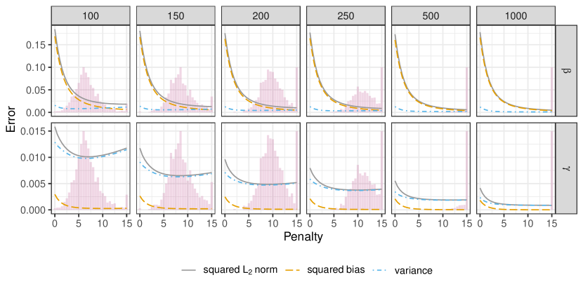
Figure 7: As Figure 3 but for estimation with SCRPS instead of LogS.

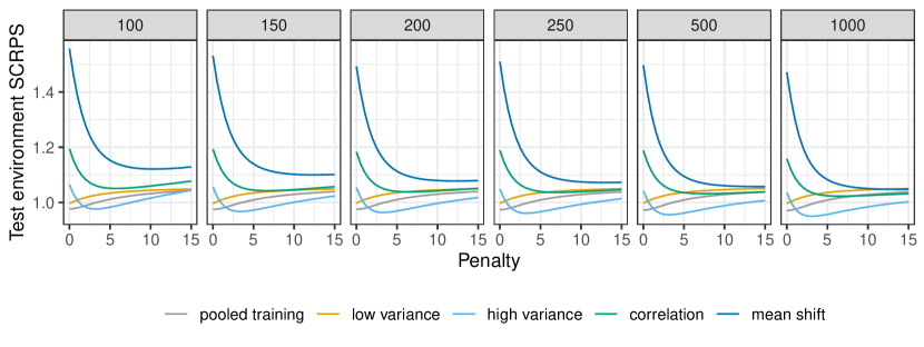
Figure 8: As Figure 4 but for estimation and evaluation with SCRPS instead of LogS.

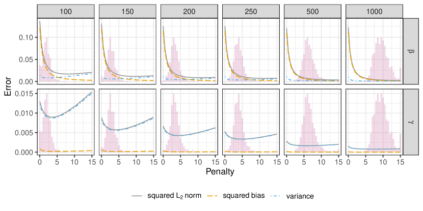
Figure 9: As Figure 3 but with $\alpha=0.01$ for choosing the penalty parameter.

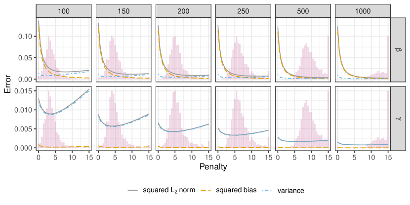
Figure 10: As Figure 3 but with $\alpha=0.1$ for choosing the penalty parameter.

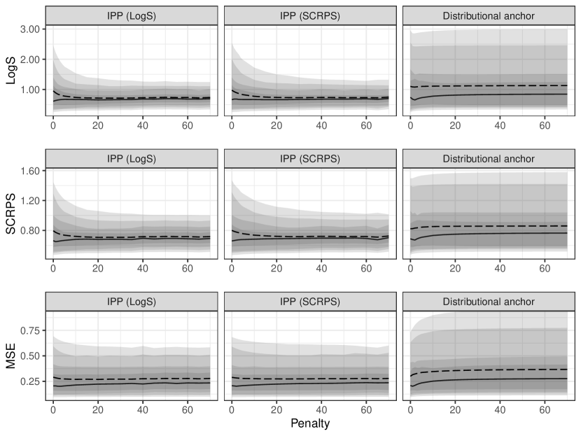
Figure 11: Comparison of IPP and distributional anchor regression when IPP excludes the observational environment.

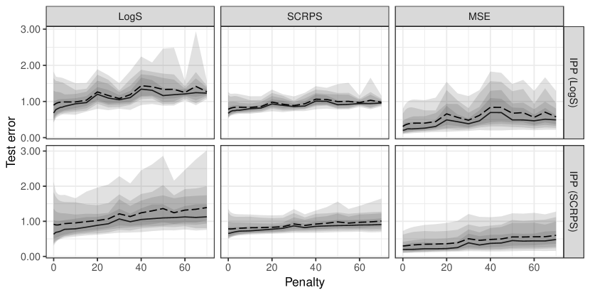
Figure 12: Scores of IPP when the environment with interventions on the response gene is included in the training data.

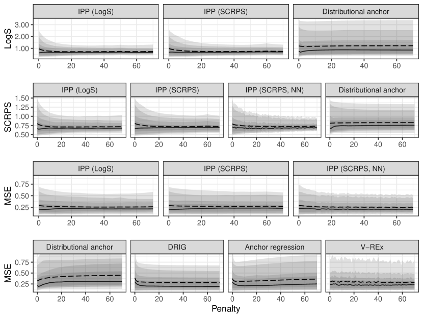
Figure 13: Same as Figure 6 but with the environment where $Y$ is intervened on included in the training data for distributional anchor regression, anchor regression, and DRIG.

References

- Arjovsky et al., (2019) Arjovsky, M., Bottou, L., Gulrajani, I., and Lopez-Paz, D. (2019). Invariant risk minimization. arXiv preprint arXiv:1907.02893.
- Bolin and Wallin, (2023) Bolin, D. and Wallin, J. (2023). Local scale invariance and robustness of proper scoring rules. Statist. Sci., 38(1):140–159.
- Bühlmann, (2020) Bühlmann, P. (2020). Invariance, causality and robustness: 2018 Neyman Lecture. Statist. Sci., 35(3):404–426.
- Christiansen et al., (2022) Christiansen, R., Pfister, N., Jakobsen, M. E., Gnecco, N., and Peters, J. (2022). A causal framework for distribution generalization. IEEE Transactions on Pattern Analysis and Machine Intelligence, 44(10):6614–6630.
- Cook and Weisberg, (1983) Cook, R. D. and Weisberg, S. (1983). Diagnostics for heteroscedasticity in regression. Biometrika, 70(1):1–10.
- Duchi and Namkoong, (2021) Duchi, J. C. and Namkoong, H. (2021). Learning models with uniform performance via distributionally robust optimization. Ann. Statist., 49(3):1378–1406.
- Gneiting, (2011) Gneiting, T. (2011). Making and evaluating point forecasts. Journal of the American Statistical Association, 106(494):746–762.
- Gneiting and Raftery, (2007) Gneiting, T. and Raftery, A. E. (2007). Strictly proper scoring rules, prediction, and estimation. J. Amer. Statist. Assoc., 102(477):359–378.
- Henzi et al., (2023) Henzi, A., Kleger, G.-R., and Ziegel, J. F. (2023). Distributional (single) index models. J. Amer. Statist. Assoc., 118(541):489–503.
- Hyvärinen, (2005) Hyvärinen, A. (2005). Estimation of non-normalized statistical models by score matching. J. Mach. Learn. Res., 6:695–709.
- Jakobsen and Peters, (2021) Jakobsen, M. E. and Peters, J. (2021). Distributional robustness of K-class estimators and the PULSE. The Econometrics Journal, 25(2):404–432.
- Kingma and Ba, (2015) Kingma, D. P. and Ba, J. (2015). Adam: A method for stochastic optimization. In Proceedings of the 3rd International Conference on Learning Representations (ICLR).
- Kneib et al., (2023) Kneib, T., Silbersdorff, A., and Säfken, B. (2023). Rage against the mean—a review of distributional regression approaches. Econom. Stat., 26:99–123.
- Kook et al., (2022) Kook, L., Sick, B., and Bühlmann, P. (2022). Distributional anchor regression. Stat. Comput., 32(3):Paper No. 39, 19.
- Krueger et al., (2021) Krueger, D., Caballero, E., Jacobsen, J.-H., Zhang, A., Binas, J., Zhang, D., Le Priol, R., and Courville, A. (2021). Out-of-distribution generalization via risk extrapolation (REx). In International Conference on Machine Learning, pages 5815–5826. PMLR.
- Ledoux and Talagrand, (1988) Ledoux, M. and Talagrand, M. (1988). Characterization of the law of the iterated logarithm in Banach spaces. Ann. Probab., 16(3):1242–1264.
- Meinshausen, (2018) Meinshausen, N. (2018). Causality from a distributional robustness point of view. In 2018 IEEE Data Science Workshop (DSW), pages 6–10.
- Murphy and Daan, (1985) Murphy, A. H. and Daan, H. (1985). Forecast evaluation. Probability, statistics, and decision making in the atmospheric sciences, pages 1—547.
- Paszke et al., (2019) Paszke, A., Gross, S., Massa, F., Lerer, A., Bradbury, J., Chanan, G., Killeen, T., Lin, Z., Gimelshein, N., Antiga, L., et al. (2019). Pytorch: An imperative style, high-performance deep learning library. Advances in neural information processing systems, 32.
- Peters et al., (2016) Peters, J., Bühlmann, P., and Meinshausen, N. (2016). Causal inference by using invariant prediction: identification and confidence intervals. J. R. Stat. Soc. Ser. B. Stat. Methodol., 78(5):947–1012. With comments and a rejoinder.
- Rojas-Carulla et al., (2018) Rojas-Carulla, M., Schölkopf, B., Turner, R., and Peters, J. (2018). Invariant models for causal transfer learning. The Journal of Machine Learning Research, 19(1):1309–1342.
- Rothenhäusler et al., (2019) Rothenhäusler, D., Bühlmann, P., and Meinshausen, N. (2019). Causal Dantzig: fast inference in linear structural equation models with hidden variables under additive interventions. Ann. Statist., 47(3):1688–1722.
- Rothenhäusler et al., (2021) Rothenhäusler, D., Meinshausen, N., Bühlmann, P., and Peters, J. (2021). Anchor regression: heterogeneous data meet causality. J. R. Stat. Soc. Ser. B. Stat. Methodol., 83(2):215–246.
- Scrucca, (2013) Scrucca, L. (2013). GA: A package for genetic algorithms in R. Journal of Statistical Software, 53(4):1–37.
- Shen et al., (2023) Shen, X., Bühlmann, P., and Taeb, A. (2023). Causality-oriented robustness: exploiting general additive interventions. arXiv e-prints, page arXiv:2307.10299.
- Shen and Meinshausen, (2023) Shen, X. and Meinshausen, N. (2023). Engression: Extrapolation for nonlinear regression? arXiv preprint arXiv:2307.00835.
- Sinha et al., (2017) Sinha, A., Namkoong, H., and Duchi, J. (2017). Certifiable distributional robustness with principled adversarial training. arXiv preprint arXiv:1710.10571.
- Székely et al., (2004) Székely, G. J., Rizzo, M. L., et al. (2004). Testing for equal distributions in high dimension. InterStat, 5(16.10):1249–1272.
- Vannitsem et al., (2020) Vannitsem, S., Bremnes, J. B., Demaeyer, J., Evans, G. R., Flowerdew, J., Hemri, S., Lerch, S., Roberts, N., Theis, S., Atencia, A., et al. (2020). Statistical postprocessing for weather forecasts–review, challenges and avenues in a big data world. Bulletin of the American Meteorological Society, pages 1–44.