Warp Drives, Rest Frame Transitions, and Closed Timelike Curves

Abstract

It is a curiosity of all warp drives in the Natário class that none allow a free-falling passenger to land smoothly on a moving destination, for example a space station or an exoplanet, as we demonstrate here. This has implications on the hypothetical practical usage of warp drives for future interstellar travel, but also raises more fundamental issues regarding the relationship between superluminal travel and time travel. We present a modification to the Natário warp drive, using a non-unit lapse function as in the ADM formalism, that removes this pathology. We also provide a thorough geometrical analysis into what exactly a warp drive needs to be able to “land”, or transition between rest frames. This is then used to give generic and explicit examples of a spacetime containing two warp drives, such that the geodesic of an observer travelling along one and then the other naturally forms a closed timelike curve. This provides a precise model for the connection between faster-than-light travel and time travel in general relativity. Alongside this, we give a detailed discussion of the weak energy condition in non-unit-lapse warp drive spacetimes.

1 Introduction

Since Alcubierre’s seminal 1994 paper [1], the warp drive has developed from a vague, science-fictional concept to a subject of genuine scientific interest [2, 3, 4]. Whilst not generally considered to be a realistic option for human interstellar travel in the near future, it serves as an interesting theoretical model, opening up new insights into the surprising possibilities that arise from the curved spacetime geometry of general relativity. Studying warp drives may also expose pathologies in the theory itself.

The idea behind a warp drive is to allow an observer following a timelike path to travel at a global speed that is, in principle, unbounded, and could potentially be greater than that of light. It takes advantage of a loophole in general relativity that, while all massive objects are constrained to move along timelike paths, space itself has no such restriction. Roughly speaking, a warp drives exploits this by having a shell of curved spacetime embedded in a flat background spacetime that can accelerate its flat interior to arbitrarily high speeds, without the passengers inside feeling any acceleration whatsoever.

There are numerous problems with warp drives as they have so far been conceived, even setting aside the extreme engineering difficulties. The most notable are their seemingly-inevitable violation of the energy conditions [5, 6], the typically vast amounts of (negative) energy required to sustain them [1, 7], and the formation of event horizons [1, 8].

In this paper, we consider a further and as-yet unremarked upon pathology present in generic warps drives of the Natário class [9], namely their inability to perform rest frame transitions. We define a rest frame transition, loosely, as the net acceleration of a free-falling observer from being at rest in one frame of reference to being at rest in another, using spacetime curvature in a manner similar to that of a warp drive. This is what would be necessary in order to land a warp drive on a moving target, for example.

To the authors’ knowledge, nobody has yet commented on this curious fact. For example, take an Alcubierre warp drive, defined by the metric

$$\mathop{}\!\mathrm{d}s^{2}=-\mathop{}\!\mathrm{d}t^{2}+\mathop{}\!\mathrm{d}x^{2}+\mathop{}\!\mathrm{d}y^{2}+(\mathop{}\!\mathrm{d}z-fv\mathop{}\!\mathrm{d}t)^{2}$$ (1.1)

where $f=f(x,y,z-\zeta(t))$ with $f(0,0,0)=1$, $f\rightarrow 0$ at spatial infinity, and $v(t)=\partial_{t}\zeta(t)$. Note that this metric is only flat in the vicinity of a hypersurface $t=\text{constant}$ if $v(t)=0$. It can easily be shown that the path

$$\alpha(\tau)=(\tau,0,0,\zeta(\tau)),\qquad\tau\in(-\infty,\infty)$$ (1.2)

is a geodesic, parameterised by proper time $\tau$.

Now consider the case that $\zeta(t)=0\implies v(t)=0$ for $t\leq 0$. Then a passenger of the warp drive following this geodesic would begin at rest in some reference frame $S$ described by the coordinates $(t,x,y,z)$, in an entirely flat universe (for $t\leq 0$). Suppose that an intrepid but regrettably naive traveller wants to use this warp drive to travel to a distant star which is moving along the $z$ axis at some speed $0<u<1$ in the Earth’s rest frame. If they are to complete this journey and start their new life on an exoplanet orbiting the star, they may imagine they can use a warp drive described by (1.1) and simply choose $v(t)$ such that when they reach the star, $v(t)=u$, allowing them to arrive without issue.

However, on arrival, they will find themselves faced with an unpleasant surprise: they cannot land on the exoplanet. The reason for this is that the spacetime curvature surrounding them vanishes only if $v\left(t\right)=0$, so they cannot simply leave the warp drive unless it decelerates back to its original starting velocity. Therefore, they would have had to have brought a rocket or some other form of artificial propulsion with them in order to reaccelerate themselves back up to the speed $u$. It turns out to be not as trivial as one would expect to “flatten the surrounding curvature” without decelerating the traveller inside back to rest in $S$.

There seems to be no reason why such a strange, two-stage journey should be necessary. However, as we show in Section 2, a surprisingly wide class of warp drives suffers from the same issue. In Section 3, we present a solution to this problem by introducing a particular non-unit lapse function, and save our interstellar traveller a lot of hassle.

The other reason that the study of rest frame transitions is important is that it sheds light on the well-known relationship between superluminal travel and time travel. This connection is by no means set in stone, and is a subtle topic. In this paper, we shall consider the following well-known way of using superluminal travel to facilitate time travel.

Consider two reference frames $S$ and $S^{\prime}$, with some relative velocity $u$ along the $x$ axis. Suppose superluminal travel in a warp drive is possible, and that one can travel a large distance at an average speed $v>1$ in a given reference frame. Then, if $u$ is large enough for a given $v$, one can travel back in time by travelling superluminally between two points in the $S$ frame, transitioning to the $S^{\prime}$ frame, and returning superluminally in the $S^{\prime}$ frame to the starting point.

This is proven mathematically in Section 4.2, but it is visually clear from the spacetime diagram in Figure 1.1. Here, the traveller uses two warp drives to follow the path of the blue arrows, which both represent superluminal paths in $S$ and $S^{\prime}$ respectively. First, they travel from $x=0$ out along the upper arrow, finishing at a speed $u$ and perhaps landing on a space station at rest in $S^{\prime}$. Then, they travel back along the lower arrow. The traveller arrives back at $x=0$ earlier than when they left, so they have travelled backwards in time.

Note that along the upper arrow, moving in the positive $x$ direction, the traveller is moving forwards in time according to $S$, but backwards in time according to $S^{\prime}$. Similarly, along the lower arrow, moving in the negative $x$ direction, the traveller is moving forwards in time according to $S^{\prime}$, but backwards in time according to $S$. This is how the “trick” works: for any object moving superluminally in one frame of reference, there is another frame of reference in which they are moving backwards in time.

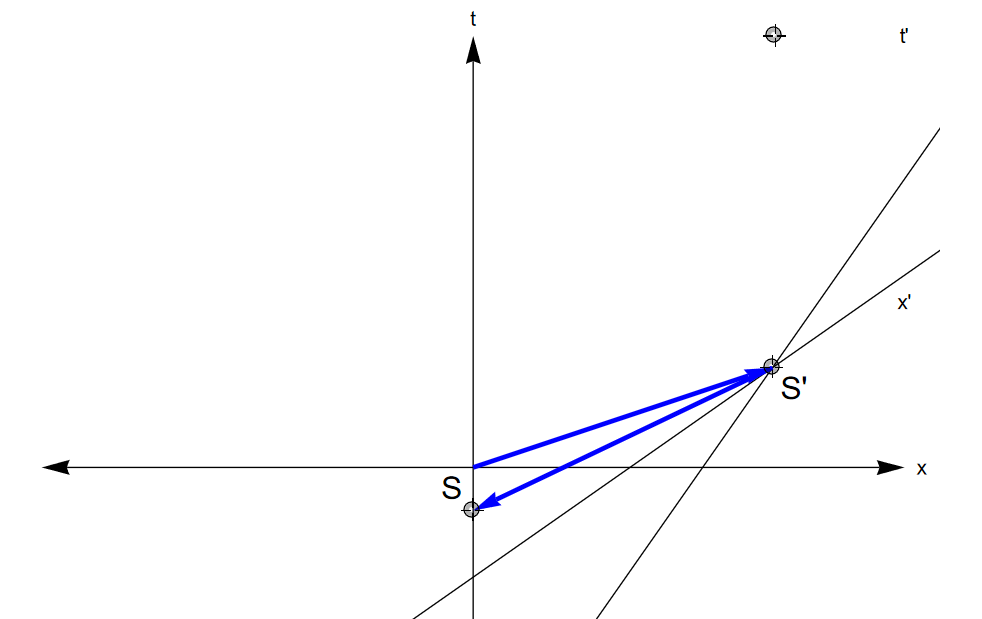
Figure 1.1: Spacetime diagram showing how superluminal travel may allow for time travel. In the unprimed coordinates (representing $S$), the path moving in the positive $x$ direction is moving forwards in $t$, and in the primed coordinates (representing $S^{\prime}$), the path moving along the negative $x$ direction is moving forwards in $t^{\prime}$. However, each path viewed in the other frame is travelling backwards in their respective time coordinates. Here the relative velocity between the frames is $u=0.7$, and the speed of the warp drive in both directions is $v=3$.

A somewhat messy calculation pertaining to this idea was performed in [10], later repeated in [11], but there are several problems with this. The first and most serious of these is that a rest frame transition is implicitly used when the author claims that the traveller simply accelerates up to some non-zero subluminal speed in order to be at rest in the frame $S^{\prime}$. This seems dubious, as the traveller needs some artificial form of propulsion after leaving the warp drive, with the sole purpose of “changing their time coordinate”. They are not following a geodesic here.

Secondly, the warp drives used were non-compact Alcubierre drives, meaning the two warp drives overlapped. It was simply assumed that this overlapping was negligible, leaving the geodesics inside the two warp drives unaffected. Thirdly, the calculation’s purpose was only to demonstrate the principle that CTCs can arise in double warp drive spacetimes, and as such it was not performed with complete rigour, with many quantities assumed negligible.

This may seem like nit-picking. However, since we are very much in the realm of “suspect” physics, with closed timelike curves lurking nearby, it is vital to be as rigorous as possible. The rest frame transition is in a sense the tool that is used to “turn” superluminal travel into time travel, and as such, we must take great care when dealing with it.

The closed timelike curve in our double warp drive spacetime should be a geodesic everywhere, to avoid the necessity for some unspecified form of artificial propulsion. A Natário warp drive will not by itself allow for this, as we shall show shortly. Therefore, in Section 4, we present an explicit metric describing a double warp drive spacetime which contains a closed timelike geodesic. The two warp drives do not overlap at all, so there is no assumption that the interference is insignificant. This gives a much more solid foundation to the widely-held belief that faster-than-light travel allows for time travel.

In Section 5, we give a discussion of recent and previous work on the violation of the pointwise weak energy condition (WEC) in warp drive spacetimes, in particular [6], [15], [16], [17], [18] and [19]. We particularly focus on arguments presented in [6], and extend the arguments therein to allow for a non-unit lapse function.

We find that this does not help to avoid WEC violations, subject to some reasonable conditions. We also give an analysis of the case of zero Eulerian energy density and a curl-free shift vector field, as this was not accounted for in [6]. We conclude that the WEC violations are likely nothing more than an artefact of the class of metrics, and have nothing to do with the metrics’ potential to describe warp drives.

This paper introduces many different mathematical symbols. To prevent confusion and help make the mathematical formulas presented in the paper more clear, we provide a convenient table of symbols in Appendix C. We denote 4-dimensional spacetime indices using Greek letters, and 3-dimensional spatial indices using lowercase English letters.

Throughout the paper, we have used both the Mathematica package OGRe (An Object-Oriented General Relativity Package) [20] and a beta version of the Python package OGRePy [21] to facilitate calculations of curvature tensors, geodesics, and other relevant geometrical quantities.

2 Natário drives cannot perform rest frame transitions

First, we give a preliminary definition of a rest frame transition, which will suffice for our purposes in Sections 2 - 6. We subsequently give a more general definition and thorough analysis in Section 7, beginning from a coordinate-independent starting point.

We take a general metric $g_{\mu\nu}$ expressed in the ADM formalism and coordinates $(t,x,y,z)$ as

$$\mathop{}\!\mathrm{d}s^{2}=-N^{2}\mathop{}\!\mathrm{d}t^{2}+\gamma_{ij}(\mathop{}\!\mathrm{d}x^{i}-\beta^{i}\mathop{}\!\mathrm{d}t)(\mathop{}\!\mathrm{d}x^{j}-\beta^{j}\mathop{}\!\mathrm{d}t)$$ (2.1)

The metric is assumed to be asymptotically flat in these coordinates, that is, as $r\equiv\sqrt{x^{2}+y^{2}+z^{2}}\rightarrow\infty$,

$$\begin{gathered}N\rightarrow 1,\\ \bm{\beta}\rightarrow\mathbf{0},\\ \gamma_{ij}\rightarrow\delta_{ij}.\end{gathered}$$ (2.2)

We say that (2.1) allows for a rest frame transition if:

1. $\exists T_{flat}>0$ such that if $t\in(-\infty,0]\cup[T_{flat},\infty)$, $g_{\mu\nu}=\eta_{\mu\nu}$, where $\eta_{\mu\nu}$ is the Minkowski metric.

2. There exists a timelike geodesic $\Gamma_{RFT}$ such that for $t\leq 0$, $\Gamma_{RFT}$ has tangent vector $v^{\mu}=(1,\mathbf{0})$ and that for $t\geq T_{flat}$, $\Gamma_{RFT}$ has tangent vector $v^{\mu}\neq(1,\mathbf{0}).$

For $t\notin(0,T_{flat})$, the coordinates $(t,x,y,z)$ describe an inertial reference frame, since $g_{\mu\nu}=\eta_{\mu\nu}$. This encapsulates the idea of an observer starting at rest in this reference frame and finishing at rest in a different reference frame.

We shall now demonstrate the entire class of Natário warp drives does not allow for rest frame transitions. The Natário class is the set of asymptotically-flat spacetimes with metric (2.1) but setting $N=1,\gamma_{ij}=\delta_{ij}$:

$$\mathop{}\!\mathrm{d}s^{2}=-\mathop{}\!\mathrm{d}t^{2}+\delta_{ij}(\mathop{}\!\mathrm{d}x^{i}-\beta^{i}\mathop{}\!\mathrm{d}t)(\mathop{}\!\mathrm{d}x^{j}-\beta^{j}\mathop{}\!\mathrm{d}t).$$ (2.3)

Define $\Sigma_{t^{*}}\equiv t^{-1}(t^{*})$ for $t^{*}\in\mathbb{R}$. The normal vector field to $\Sigma_{t}$ is given by

$$\begin{gathered}\mathbf{n}\equiv-\mathop{}\!\mathrm{d}t\\ \implies n_{\mu}=(-1,\mathbf{0}),\qquad n^{\mu}=(1,\bm{\beta}).\end{gathered}$$ (2.4)

Consider an observer starting at rest in the rest frame described by these coordinates at a time $t<0$, with 4-velocity $(1,0,0,0)$ (as they would along $\Gamma_{RFT}$, if it exists). This means that the observer is initially Eulerian, by which we mean that their 4-velocity coincides with the normal vector field. Consider the following general formula (proven in Appendix B), valid in any ADM spacetime:

$$n^{\nu}\nabla_{\nu}n_{\mu}=\frac{1}{N}(\nabla_{\mu}N+n_{\mu}\mathcal{L}_{\mathbf{n}}N),$$ (2.5)

where $\mathcal{L}$ denotes the Lie derivative. From this formula, one can easily show that the integral curves of the vector field $n^{\mu}$ (the paths of Eulerian observers) are geodesics if and only if $\partial_{i}N=0\iff N=N(t)$. This is clearly the case for (2.3), so the observer, wherever they go, must have 4-velocity $n^{\mu}$.

By the expressions for a general metric expressed in the ADM formalism given in Appendix A, Equation (A.2), we can see that

$$n^{\mu}=-Ng^{0\mu}=-g^{0\mu},$$ (2.6)

since, as $t\rightarrow T_{flat}$, $g^{0\mu}\rightarrow\eta^{0\mu}=(-1,0,0,0)$ and $n^{\mu}\rightarrow(1,\mathbf{0})$. The observer must have this same 4-velocity, and we see that they have returned to being at rest in the original frame of reference. Therefore, (2.3) does not allow for rest frame transitions, and could not be used to land on a moving target. $\Box$

The above argument can easily be extended to the case where $N=N(t)$, $\delta_{ij}\rightarrow\gamma_{ij}$ for arbitrary $N(t)>0$ and positive-definite $\gamma_{ij}$, since Eulerian observers still follow geodesics and we must still have $n^{\mu}\rightarrow(1,\mathbf{0})$ as $t\rightarrow T_{flat}$. Therefore, in order to find a metric allowing for a rest frame transition, we have no choice but to introduce spatial dependence into the lapse. This will be the subject of the next chapter.

3 A warp drive allowing for a rest frame transition

In this section, we introduce a general warp drive that starts from rest in some reference frame and travels along an arbitrary path $\mathbf{r}(t)$ for $0<t<T_{1}$ where $T_{1}>0$, finishing at a constant 3-velocity $(0,0,u)$ for $t\geq T_{1}$. We then show how we can manipulate the metric so that the warp curvature flattens whilst keeping the free-falling passengers moving at a speed $u$ along the $z$ axis. This means that we have found a warp drive capable of landing on a target moving at a speed $u$.

First, we introduce a generic warp drive following an arbitrary path $\mathbf{r}(t)=(X(t),Y(t),Z(t))$, with a shift vector $\bm{\beta}=a(t)\mathbf{v}(t,\mathbf{x})$. We set $\partial_{t}\mathbf{r}(t)=\mathbf{v}(t,\mathbf{r}(t))$ so that $(t,\mathbf{r}(t))$ is an integral curve of $(1,\mathbf{v}(t,\mathbf{x}))$. Our new metric is given by

$$\mathop{}\!\mathrm{d}s^{2}=-N^{2}\mathop{}\!\mathrm{d}t^{2}+\delta_{ij}(\mathop{}\!\mathrm{d}x^{i}-\beta^{i}\mathop{}\!\mathrm{d}t)(\mathop{}\!\mathrm{d}x^{j}-\beta^{j}\mathop{}\!\mathrm{d}t).$$ (3.1)

The introduction of $a$ and a non-unit lapse $N$ are our modifications to the Natário form of the metric, and their significance shall soon become clear. We also set $\mathbf{v}$ such that

$$(\partial_{i}v^{j})(t,\mathbf{r}(t))=0,$$ (3.2)

that is, $\mathbf{v}$ is flat at the warp drive centre $(t,\mathbf{r}(t))$, and as usual, we also require $\mathbf{v}\rightarrow\mathbf{0}$ at spatial infinity. All functions describing the metric are assumed to be at least $C^{2}$, such that the Riemann tensor is continuous.

The geodesic Lagrangian is

$$\mathcal{L}_{g}=\frac{1}{2}\left(-N^{2}\dot{t}^{2}+\delta_{ij}(\dot{x}^{i}-\beta^{i}\dot{t})(\dot{x}^{j}-\beta^{j}\dot{t})\right),$$ (3.3)

where we shall use $\cdot$ to denote differentiation with respect to proper time $\tau$. The Euler-Lagrange equations then imply

$$\begin{gathered}0=\frac{\mathop{}\!\mathrm{d}}{\mathop{}\!\mathrm{d}\tau}(-N^{2}\dot{t}-\delta_{jk}\beta^{j}(\dot{x}^{k}-\beta^{k}\dot{t}))+\dot{t}^{2}N\partial_{t}N+\dot{t}\cdot\delta_{jk}(\partial_{t}\beta^{j})(\dot{x}^{k}-\beta^{k}\dot{t}),\\ 0=\frac{\mathop{}\!\mathrm{d}}{\mathop{}\!\mathrm{d}\tau}(\dot{x}^{i}-\beta^{i}\dot{t})+\dot{t}^{2}N\partial_{x^{i}}N+\dot{t}\cdot\delta_{jk}(\partial_{x^{i}}\beta^{j})(\dot{x}^{k}-\beta^{k}\dot{t}).\end{gathered}$$ (3.4)

The unit normal vector field to hypersurfaces of constant $t$, $\Sigma_{t}$, is given by

$$\mathbf{n}\equiv-N\mathop{}\!\mathrm{d}t\quad\implies\quad n_{\mu}=(-N,\mathbf{0}),\qquad n^{\mu}=\frac{1}{N}(1,\bm{\beta}).$$ (3.5)

Again, an integral curve of this vector field will satisfy the geodesic equations if and only if $\partial_{i}N=\mathbf{0}$, as can be seen from (3.4). The path $(\tau,\mathbf{r}(\tau))$ is thus a geodesic wherever $N=1$ and $a=1$, as it is an integral curve of $n^{\mu}$. It is also parameterised by proper time.

Now take $0<T_{1}<T_{2}$ and consider the case that

$$\begin{cases}\mathbf{v}(t,\mathbf{x})=\mathbf{0}&t\leq 0,\ \mathbf{x}\in\mathbb{R}^{3},\\ \mathbf{v}(t,\mathbf{r}(t))=(0,0,u)&t\geq T_{1},\end{cases}$$ (3.6)

for some fixed $0<u<1$, and $\mathbf{v}$ is unconstrained for $0<t<T_{1}$. We take $a(t)$ as follows:

$$\begin{cases}a(t)=1&t\leq T_{1},\\ 0<a(t)<1&T_{1}<t<T_{2},\\ a(t)=0&t\geq T_{2},\end{cases}$$ (3.7)

and set the lapse as

$$N=1-b\cdot(z-Z)s.$$ (3.8)

where $s\rightarrow 0$ at spatial infinity with $s(t,\mathbf{r}(t))=1$, $(\partial_{i}s)(t,\mathbf{r}(t))=0$ and

$$\begin{gathered}b(t)\equiv-u\lambda^{2}\cdot\partial_{t}a,\\ \lambda\equiv(1-u^{2}(1-a)^{2})^{-\frac{1}{2}}.\end{gathered}$$ (3.9)

We call $a$ and $b$ the transition functions for the shift vector and lapse respectively. $s$ and $a$ must also be chosen such that $N>0$ everywhere.

Note that for $t\geq T_{2}$, $a$ and $b$ vanish, so $g_{\mu\nu}=\eta_{\mu\nu}$, and the metric becomes Minkowskian (so $T_{2}$ corresponds to $T_{flat}$ in the previous section). $b(t)$ vanishes for $t\notin(T_{1},T_{2})$, so $N=1$ for $t\notin(T_{1},T_{2})$, and Eulerian observers follow geodesics here, so taking

$$\chi_{1}(\tau)\equiv(\tau,\mathbf{r}(\tau)),\qquad 0\leq\tau\leq\tau_{1}\equiv T_{1},$$ (3.10)

we see $\chi_{1}([0,\tau_{1}])$ is a geodesic. However, in the region with $t\in(T_{1},T_{2})$, Eulerian observers do not follow geodesics. For $T_{1}\leq t\leq T_{2}$, consider the path $\chi_{2}$ satisfying

$$\begin{gathered}\dot{\chi_{2}}(\tau)=(\lambda,0,0,\lambda u),\\ \chi_{2}(\tau_{1})=(T_{1},\mathbf{r}(T_{1})),\end{gathered}$$ (3.11)

so that at $\tau=\tau_{1}>0$, $a$ may start to change. Since $0\leq a\leq 1$ and $|u|<1$,

$$1\leq\lambda\leq\gamma_{u}\equiv(1-u^{2})^{-\frac{1}{2}},$$ (3.12)

and this ordinary differential equation has a unique, smooth solution for all $\tau\geq\tau_{1}$. We now demonstrate that the solution to (3.11) is a geodesic.

For $\chi_{2}$,

$$\frac{\mathop{}\!\mathrm{d}z}{\mathop{}\!\mathrm{d}t}=\frac{\mathop{}\!\mathrm{d}z}{\mathop{}\!\mathrm{d}\tau}\cdot\frac{\mathop{}\!\mathrm{d}\tau}{\mathop{}\!\mathrm{d}t}=\lambda u\cdot\frac{1}{\lambda}=u,$$ (3.13)

so parameterised by coordinate time, this is the path

$$(\chi_{2}\circ\tau)(t)=(t,X(T_{1}),Y(T_{1}),Z(T_{1})+u(t-T_{1}))=(t,\mathbf{r}(t)),$$ (3.14)

and looking at (3.8), $N=1$ along this path (but crucially, $\partial_{z}N\neq 0$). As can be checked from (3.1), this has the consequence that $\dot{\chi}_{2}$ is normalised, i.e. $g(\dot{\chi}_{2},\dot{\chi}_{2})=-1$, and we see that $\tau$ is the proper time of the path, with

$$\tau(t)=T_{1}+\int_{T_{1}}^{t}\sqrt{-g(\partial_{t}\chi_{2},\partial_{t}\chi_{2})}\mathop{}\!\mathrm{d}t^{\prime},\qquad T_{1}<t\leq T_{2}.$$ (3.15)

Taking the first geodesic equation, along $\chi_{2}$, we have

$$0 =\frac{\mathop{}\!\mathrm{d}}{\mathop{}\!\mathrm{d}\tau}(-1^{2}\cdot\lambda-\lambda\cdot(u-au)\cdot au)+\lambda^{2}\cdot 1\cdot ub+u\lambda\partial_{t}a(\lambda u(1-a))$$ (3.16)

$$=-\frac{\mathop{}\!\mathrm{d}}{\mathop{}\!\mathrm{d}\tau}(\lambda+\lambda u^{2}a(1-a))+\lambda^{2}ub+\lambda u^{2}\frac{\mathop{}\!\mathrm{d}a}{\mathop{}\!\mathrm{d}\tau}(1-a)$$

$$=-\dot{\lambda}+\lambda^{2}ub-au^{2}\frac{\mathop{}\!\mathrm{d}}{\mathop{}\!\mathrm{d}\tau}(\lambda(1-a))$$

$$=-\dot{\lambda}-u^{2}a(1-a)\dot{\lambda}+u^{2}\lambda a\dot{a}+\lambda^{2}ub$$

$$=u^{2}\lambda\dot{a}(\lambda^{2}(1-a)+au^{2}\lambda^{2}(1-a)^{2}+au^{2})+\lambda^{2}ub$$

$$=u^{2}\lambda^{3}\dot{a}((1-a)+au^{2}(1-a)^{2}+a(1-u^{2}(1-a)^{2}))+\lambda^{2}ub$$

$$=u^{2}\lambda^{3}\dot{a}+\lambda^{2}ub$$

$$\implies 0=u\lambda^{2}\partial_{t}a+b,$$

where in the fifth line we have used the identity $\dot{\lambda}=-\lambda^{3}u^{2}(1-a)\dot{a}$, and in the sixth the definition of $\lambda$. Therefore, we see that we recover (3.9) as a necessary condition for $\chi_{2}$ to be geodesic.

The geodesic equations for $x(\tau)$ and $y(\tau)$ are trivially satisfied since, along $\chi_{2}$,

$$\dot{x}=\beta^{x}=\partial_{x}N=\dot{y}=\beta^{y}=\partial_{y}N=0.$$

So finally, considering the equation for $z(\tau)$:

$$0 =\frac{\mathop{}\!\mathrm{d}}{\mathop{}\!\mathrm{d}\tau}(\lambda u(1-a))-\lambda^{2}\cdot 1\cdot b+0$$ (3.17)

$$=\frac{\mathop{}\!\mathrm{d}}{\mathop{}\!\mathrm{d}\tau}(\lambda u(1-a))-\lambda^{2}b,$$

where we have used that $(\partial_{i}\beta^{j})(t,\mathbf{r}(t))=0\implies\partial_{z}\beta^{z}=0$ and $(\partial_{i}s)(t,\mathbf{r}(t))=0$ along $\chi_{2}$. Now looking at the third line in (3.16), we see this can be written as

$$0=\frac{1}{au}(-\dot{\lambda}+\lambda^{2}ub)-\lambda^{2}b$$ (3.18)

$$\implies 0=u\lambda^{2}\partial_{t}a+b.$$

Therefore, (3.9) is a necessary and sufficient condition for $\chi_{2}$ to be geodesic. $\Box$

Finally, we note that the combination of the two above paths

$$\chi(\tau)\equiv\begin{cases}\chi_{1}(\tau)&0\leq\tau<\tau_{1},\\ \chi_{2}(\tau)&\tau_{1}\leq\tau\leq\tau_{2},\end{cases}$$ (3.19)

where $\tau_{2}\equiv\tau(T_{2})$, is also a geodesic. This can be seen by noting that both the position and tangent vector of $\chi_{1}$ at $\tau=\tau_{1}$ match those of $\chi_{2}$ at $\tau=\tau_{1}$, so extending the geodesic $\chi_{1}$ is equivalent to solving the geodesic equation with initial conditions

$$\begin{gathered}\chi(\tau_{1})=(T_{1},\mathbf{r}(T_{1})),\\ \dot{\chi}(\tau_{1})=(1,0,0,u),\end{gathered}$$ (3.20)

which is exactly $\chi_{2}$. Written another way, the entire curve

$$\Gamma_{RFT}\equiv\{p\in M:\exists\,t\in[0,T_{2}]:p=(t,\mathbf{r}(t))\}$$ (3.21)

is a geodesic, and it satisfies the requirements described in Section 2. This means that a free-falling observer starting at rest in the centre of the bubble does not fall out of it, and their final 4-velocity at time $t=T_{2}$ is $(\gamma_{u},0,0,\gamma_{u}u)$ - not the same as their initial 4-velocity of $(1,0,0,0)$. Since, for $t\geq T_{2}$, $g_{\mu\nu}=\eta_{\mu\nu}$, we therefore see that an observer following this geodesic has transitioned between rest reference frames.

4 Making a closed timelike geodesic

4.1 General construction

In this section, we demonstrate how the above method of performing a rest frame transition may be employed to write down a metric describing a spacetime containing a closed timelike geodesic. To the authors’ knowledge, this is the first explicit example of a spacetime metric which explicitly uses superluminal travel to create a closed timelike curve, and furthermore, the closed timelike curve we find is a geodesic, requiring no additional forms of propulsion.

The idea, as described in the introduction, is to have an observer start at rest in a reference frame $S$, travel in a superluminal warp drive of the form (3.1), transition to a different reference frame $\hat{S}$, and then travel back to the starting point in a similar warp drive. It will turn out that if the two warp drives move fast enough, this will result in the observer finishing the journey at a point in the causal past of their departure.

First, we introduce a generic spacetime (which we suggestively call $M_{CTC}$) containing two warp drives that take an observer on a journey to and from rest at a given spatial point in $S$, which we shall take to be $(x,y,z)=(0,0,0)$. For the return journey, we shall need to define a warp drive in the Lorentz-boosted frame $\hat{S}$, which moves at speed $u$ along the $z$ axis with respect to $S$. We thus take the metric

$$\mathop{}\!\mathrm{d}\hat{s}^{2}=-\hat{N}^{2}\mathop{}\!\mathrm{d}\hat{t}^{2}+\delta_{\hat{i}\hat{j}}(\mathop{}\!\mathrm{d}\hat{x}^{\hat{i}}-\hat{\beta}^{\hat{i}}\mathop{}\!\mathrm{d}\hat{t})(\mathop{}\!\mathrm{d}\hat{x}^{\hat{j}}-\hat{\beta}^{\hat{j}}\mathop{}\!\mathrm{d}\hat{t}),$$ (4.1)

where $(\hat{t},\hat{x},\hat{y},\hat{z})$ is the Lorentz-boosted coordinate system, using the convention that indices with circumflexes denote $\hat{S}$ coordinates and those without denote $S$ coordinates. The functions $\hat{N}$, $\hat{\bm{\beta}}$, $\hat{\mathbf{v}}$, $\hat{a}$, $\hat{b}$, $\hat{s}$, $\hat{\mathbf{r}}$, $\hat{X}$, $\hat{Y}$, and $\hat{Z}$ are defined exactly analogously to their $S$ counterparts, but with $\hat{S}$ coordinates as their arguments. There are only two other changes:

1. The critical times, $t=0,T_{1},T_{2}$, have now become $\hat{t}=\hat{T}_{0},\hat{T}_{1},\hat{T}_{2}$ respectively.

2. $\hat{\mathbf{v}}$ is set such that the warp drive finishes at rest in $S$:

$$\begin{cases}\mathbf{\hat{v}}(\hat{t},\mathbf{\hat{x}})=\mathbf{0}&\hat{t}\leq\hat{T}_{0},\ \hat{\mathbf{x}}\in\mathbb{R}^{3},\\ \mathbf{\hat{v}}(\hat{t},\mathbf{\hat{r}}(\hat{t}))=(0,0,-u)&\hat{t}\geq\hat{T}_{1}.\end{cases}$$ (4.2)

Applying the Lorentz transformation

$$\begin{gathered}\hat{t}=\gamma_{u}(t-uz),\\ \hat{x}=x,\\ \hat{y}=y,\\ \hat{z}=\gamma_{u}(z-ut),\end{gathered}$$ (4.3)

gives the metric (4.1) in $S$ coordinates as

$$\begin{gathered}\mathop{}\!\mathrm{d}s^{2}=-\hat{N}^{2}\gamma_{u}^{2}(\mathop{}\!\mathrm{d}t-u\mathop{}\!\mathrm{d}z)^{2}+(\mathop{}\!\mathrm{d}x-\hat{\beta}^{x}\gamma_{u}(\mathop{}\!\mathrm{d}t-u\mathop{}\!\mathrm{d}z))^{2}\\ +(\mathop{}\!\mathrm{d}y-\hat{\beta}^{y}\gamma_{u}(\mathop{}\!\mathrm{d}t-u\mathop{}\!\mathrm{d}z))^{2}+\gamma_{u}^{2}((\mathop{}\!\mathrm{d}z-u\mathop{}\!\mathrm{d}t)-\hat{\beta}^{z}(\mathop{}\!\mathrm{d}t-u\mathop{}\!\mathrm{d}z))^{2}\end{gathered}$$ (4.4)

where all the functions have their arguments in terms of $S$ coordinates.

Now we put these two warp drive spacetimes together. Defining $h_{\mu\nu}$ as the perturbation to the Minkowski metric $\eta_{\mu\nu}$ that gives the metric (3.1) and the corresponding perturbation for (4.4) as $\hat{h}_{\mu\nu}$, we now consider the spacetime with metric

$$g_{\mu\nu}=\eta_{\mu\nu}+h_{\mu\nu}+\hat{h}_{\mu\nu}$$ (4.5)

This spacetime contains the two warp drives described by $h_{\mu\nu}$ and $\hat{h}_{\mu\nu}$. To avoid collision of the warp drives, we make the further assumption that, viewed as functions of $(t,x,y,z)$,

$$\operatorname{supp}\bm{\beta}\cap\operatorname{supp}\hat{\bm{\beta}}=\phi=\operatorname{supp}(N-1)\cap\operatorname{supp}(\hat{N}-1).$$

An observer having travelled inside the first warp drive must be deposited in the right place in $\hat{S}$ to be picked up by the returning warp drive. Therefore, the point $(T_{2},\mathbf{r}(T_{2}))$ must correspond to $(\hat{T}_{0},\hat{\mathbf{r}}(\hat{T}_{0}))$. Using (4.3), this means

$$\begin{gathered}\hat{T}_{0}=\gamma_{u}(T_{2}-uZ(T_{2})),\\ \hat{X}(\hat{T}_{0})=X(T_{2}),\\ \hat{Y}(\hat{T}_{0})=Y(T_{2}),\\ \hat{Z}(\hat{T}_{0})=\gamma_{u}(Z(T_{2})-uT_{2}).\end{gathered}$$ (4.6)

Note that the second warp drive does not have to leave immediately – we are free to set $\hat{\mathbf{v}}=\mathbf{0}$ for some interval of time after $\hat{t}=\hat{T}_{0}$.

We may set similar conditions for the return journey to ensure that the returning observer is deposited by the second warp drive at exactly the same spatial coordinates $(x,y,z)=(0,0,0)$ in $S$. Therefore

$$(T_{finish},\mathbf{0})\leftrightarrow(\hat{T}_{2},\hat{\mathbf{r}}(\hat{T}_{2})),$$

where $T_{finish}$ is the return time of the observer as measured in $S$. Thus we have

$$\begin{gathered}\hat{T}_{2}=\gamma_{u}T_{finish},\\ \hat{X}(\hat{T}_{2})=0,\\ \hat{Y}(\hat{T}_{2})=0,\\ \hat{Z}(\hat{T}_{2})=-\gamma_{u}uT_{finish}.\end{gathered}$$ (4.7)

4.2 CTC requirements

Now we define the outgoing and returning average speeds in the $z$ and $-\hat{z}$ directions, as measured in the warp drives’ respective frames:

$$\bar{v}^{z}\equiv\frac{Z(T_{2})}{T_{2}},$$ (4.8)

$$\hat{\bar{v}}^{z}\equiv-\frac{\hat{Z}(\hat{T}_{2})-\hat{Z}(\hat{T}_{0})}{\hat{T}_{2}-\hat{T}_{0}}.$$ (4.9)

Using (4.6) and (4.7), it is straightforward to find

$$T_{finish}=T_{2}\frac{\bar{v}^{z}+\hat{\bar{v}}^{z}-u(1+\bar{v}^{z}\hat{\bar{v}}^{z})}{\hat{\bar{v}}^{z}-u}.$$ (4.10)

Clearly, if either $\bar{v}^{z}$ or $\hat{\bar{v}}^{z}$ are less than $1$, we cannot have $T_{finish}<0$. So assuming $\bar{v}^{z},\hat{\bar{v}}^{z}>1$, we get the time-travel condition:

$$u>\frac{\bar{v}^{z}+\hat{\bar{v}}^{z}}{1+\bar{v}^{z}\hat{\bar{v}}^{z}}.$$ (4.11)

Assume $T_{finish}<0$. We define the connection between these two paths at the origin in $S$

$$C\equiv\{(t,\mathbf{0}):t\in[T_{finish},0)\},$$ (4.12)

and note that the entire path given by

$$\Gamma_{CTC}\equiv\Gamma_{RFT}\cup\hat{\Gamma}_{RFT}\cup C,$$ (4.13)

where $\Gamma_{RFT}$ and $\hat{\Gamma}_{RFT}$ are defined analogously to (3.21), is a geodesic.

Since the supports of the relevant functions do not overlap, the analysis from Section 3 still holds. Therefore, we already know that $\Gamma_{RFT}$ and $\hat{\Gamma}_{RFT}$ are geodesics, and that this path is continuous at the intersections by (4.6), (4.7), (4.12). Similarly to how we proved that

$$\Gamma_{RFT}=\chi_{1}([0,\tau_{1}))\cup\chi_{2}([\tau_{1},\tau_{2}])$$

is a geodesic in Section 3, the only other thing we have to check is that the tangent vectors at the start and end points also match, which turns out to be the case. In $S$, the observer finishes the outgoing journey with 4-velocity $(\gamma_{u},0,0,u\gamma_{u})$ which, in $\hat{S}$, is $(1,0,0,0)$, agreeing with (4.2). Similarly, the observer finishes the return journey with 4-velocity $(\gamma_{u},0,0,-u\gamma_{u})$ in $\hat{S}$, which in $S$, is $(1,0,0,0)$, agreeing with (4.12) and (3.6). Thus $\Gamma_{CTC}$ is a geodesic. $\Box$

For definiteness, we now also consider the proper time $\tau$ and its relation to coordinate time $t$. This will give insight into the points at which the observer is travelling backwards in time, according to $S$. Within $\Gamma_{RFT}$, we can use the same $t(\tau)$ that we did in Section 3, that is,

$$t(\tau)=\begin{cases}\tau&\tau\in[0,\tau_{1}),\\ \tau_{1}+\epsilon^{-1}(\tau)&\tau\in[\tau_{1},\tau_{2}),\end{cases}$$ (4.14)

where

$$\begin{gathered}\epsilon(t)\equiv\int_{T_{1}}^{t}\sqrt{-g(\partial_{t}\chi,\partial_{t}\chi)}\mathop{}\!\mathrm{d}t^{\prime},\qquad t\in[T_{1},T_{2}],\\ \tau_{2}\equiv\tau_{1}+\epsilon(T_{2}).\end{gathered}$$ (4.15)

We can then similarly define $\hat{\epsilon}(\hat{t})$ along with

$$\begin{gathered}\tau_{3}=\tau_{2}+\hat{T}_{1}-\hat{T}_{0},\\ \tau_{4}=\tau_{3}+\hat{\epsilon}(\hat{T}_{2}).\end{gathered}$$ (4.16)

$\tau_{4}$ is the total proper time experienced by the observer in one round trip along $\Gamma_{CTC}$. This gives us the full description of the coordinate times $t$ and $\hat{t}$ in terms of the proper time $\tau$ along $\Gamma_{CTC}$:

$$\begin{gathered}t(\tau)=\begin{cases}\tau&\tau\in[0,\tau_{1}),\\ T_{1}+\epsilon^{-1}(\tau)&\tau\in[\tau_{1},\tau_{2}),\end{cases}\\ \hat{t}(\tau)=\begin{cases}\hat{T}_{0}+(\tau-\tau_{2})&\tau\in[\tau_{2},\tau_{3}),\\ \hat{T}_{1}+\hat{\epsilon}^{-1}(\tau)&\tau\in[\tau_{3},\tau_{4}].\end{cases}\end{gathered}$$ (4.17)

Then, using the reverse Lorentz transformation, the point $(\hat{t},\hat{\mathbf{r}}(\hat{t}))$ in $\hat{S}$ has time coordinate

$$t=\gamma_{u}(\hat{t}+u\hat{Z}(\hat{t})),$$ (4.18)

and we find the full expression for $t(\tau)$:

$$t(\tau)=\begin{cases}\tau&\tau\in[0,\tau_{1}),\\ T_{1}+\epsilon^{-1}(\tau)&\tau\in[\tau_{1},\tau_{2}),\\ \gamma_{u}(\hat{T}_{0}+(\tau-\tau_{2})+u\hat{Z}(\hat{T}_{0}+(\tau-\tau_{2})))&\tau\in[\tau_{2},\tau_{3}),\\ \gamma_{u}(\hat{T}_{1}+\hat{\epsilon}^{-1}(\tau)+u\hat{Z}(\hat{T}_{1}+\hat{\epsilon}^{-1}(\tau))&\tau\in[\tau_{3},\tau_{4}).\end{cases}$$ (4.19)

As expected, one can show that $\dot{t}(\tau)>0$ for $\tau\notin(\tau_{2},\tau_{3})$, and that for $\tau\in(\tau_{2},\tau_{3})$

$$\dot{t}(\tau)<0\iff\partial_{\hat{t}}\hat{Z}(\hat{T}_{0}+(\tau-\tau_{2}))<-\frac{1}{u}<-1,$$ (4.20)

so in order to be travelling backwards in time in $S$, the observer must be moving faster than $\frac{1}{u}$ in $\hat{S}$ in the negative $\hat{z}$ direction.

4.3 The curvature tensors

In this section, we give the curvature tensors associated with the metric (4.5). Since the metric is defined piecewise on disjoint regions of $M_{CTC}$, we can safely write

$$\prescript{(CTC)}{}{\tensor{R}{{}_{\rho\sigma\mu\nu}}}=\tensor{R}{{}_{\rho\sigma\mu\nu}}+\tensor{\hat{R}}{{}_{\rho\sigma\mu\nu}},$$ (4.21)

where $\tensor{R}{{}_{\rho\sigma\mu\nu}}$ and $\tensor{\hat{R}}{{}_{\rho\sigma\mu\nu}}$ are the Riemann tensors associated to (3.1) and (4.4).

For this, we shall need the extrinsic curvatures of the spacelike hypersurfaces defined by constant time $\Sigma_{t}$ and $\hat{\Sigma}_{\hat{t}}$, and it will be simplest to define them each in their respective frames as follows:

$$\begin{gathered}n_{\mu}=(-N,\mathbf{0}),\\ \gamma_{\mu\nu}\equiv\eta_{\mu\nu}+h_{\mu\nu}+n_{\mu}n_{\nu},\\ K_{\mu\nu}\equiv\frac{1}{2}\mathcal{L}_{\mathbf{n}}\gamma_{\mu\nu},\end{gathered}$$ (4.22)

for the outgoing warp drive in $S$ coordinates and

$$\begin{gathered}\hat{n}_{\hat{\mu}}=(-\hat{N},\mathbf{0}),\\ \hat{\gamma}_{\hat{\mu}\hat{\nu}}\equiv\eta_{\hat{\mu}\hat{\nu}}+\hat{h}_{\hat{\mu}\hat{\nu}}+\hat{n}_{\hat{\mu}}\hat{n}_{\hat{\nu}},\\ \hat{K}_{\hat{\mu}\hat{\nu}}\equiv\frac{1}{2}\mathcal{L}_{\hat{\mathbf{n}}}\hat{\gamma}_{\hat{\mu}\hat{\nu}},\end{gathered}$$ (4.23)

for the returning warp drive in $\hat{S}$ coordinates.

We shall make use of the Gauss, Codazzi, and Ricci equations, given here in general:

$$\tensor{\gamma}{{}_{\rho}^{\alpha}}\tensor{\gamma}{{}_{\sigma}^{\beta}}\tensor{\gamma}{{}_{\mu}^{\gamma}}\tensor{\gamma}{{}_{\nu}^{\delta}}\prescript{(4)}{}{R}_{\alpha\beta\gamma\delta}=\prescript{(3)}{}{R}_{\rho\sigma\mu\nu}+K_{\rho\mu}K_{\sigma\nu}-K_{\rho\nu}K_{\sigma\mu},$$ (4.24)

$$\tensor{\gamma}{{}_{\rho}^{\alpha}}n^{\beta}\tensor{\gamma}{{}_{\mu}^{\gamma}}\tensor{\gamma}{{}_{\nu}^{\delta}}\prescript{(4)}{}{R}_{\alpha\beta\gamma\delta}=D_{\mu}K_{\rho\nu}-D_{\nu}K_{\rho\mu},$$ (4.25)

$$\tensor{\gamma}{{}_{\alpha}^{\rho}}n^{\sigma}\tensor{\gamma}{{}_{\beta}^{\mu}}n^{\nu}\prescript{(4)}{}{R}_{\rho\sigma\mu\nu}=-\mathcal{L}_{\mathbf{n}}K_{\alpha\beta}+\frac{1}{N}D_{\alpha}D_{\beta}N+K_{\alpha\rho}\tensor{K}{{}_{\beta}^{\rho}},$$ (4.26)

where $D$ is the induced covariant derivative on the hypersurface in question, and $\prescript{(4)}{}{R}_{\rho\sigma\mu\nu},\prescript{(3)}{}{R}_{\rho\sigma\mu\nu}$ are the full and induced Riemann tensors respectively.

In the following, as in [6], instead of using the coordinate basis

$$\{\partial_{t},\partial_{x},\partial_{y},\partial_{z}\}$$

to specify the components of tensors, we shall use the non-coordinate, orthonormal basis

$$\{\mathbf{n},\partial_{x},\partial_{y},\partial_{z}\}$$ (4.27)

as this will allow us to use Equations (4.24)-(4.26) directly. Our notation will be such that a tensor with an index $n$ means that that index has been contracted with $n^{\mu}$, for example $R_{\mu n}\equiv R_{\mu\rho}n^{\rho}$.

It turns out that $K_{ij}$ takes a pleasingly simple form, as derived in Appendix B:

$$K_{ij}=\frac{1}{N}\partial_{(i}\beta_{j)},$$ (4.28)

and with this in mind, we evaluate $\tensor{R}{{}_{\rho\sigma\mu\nu}}$. Since the induced metric is flat, $\gamma_{ij}=\delta_{ij}$, we have $D_{i}=\partial_{i}$ and $\prescript{(3)}{}{R}_{\rho\sigma\mu\nu}=0$. Also noting that $\tensor{\gamma}{{}_{i}^{\rho}}=\tensor{\delta}{{}_{i}^{\rho}}$, Equations (4.24) - (4.26) give us, as detailed in Appendix A:

$$R_{ijkl} =K_{ik}K_{jl}-K_{il}K_{jk},$$ (4.29)

$$R_{inkl} =\tensor{\gamma}{{}_{i}^{\alpha}}n^{\beta}\tensor{\gamma}{{}_{k}^{\gamma}}\tensor{\gamma}{{}_{l}^{\delta}}R_{\alpha\beta\gamma\delta}=\partial_{k}K_{il}-\partial_{l}K_{ik},$$

$$R_{injn} =\tensor{\gamma}{{}_{i}^{\rho}}n^{\sigma}\tensor{\gamma}{{}_{j}^{\mu}}n^{\nu}R_{\rho\sigma\mu\nu}=-\mathcal{L}_{\mathbf{n}}K_{ij}+K_{ik}\tensor{K}{{}_{j}^{k}}+\frac{1}{N}\partial_{i}\partial_{j}N.$$

In contracting these expressions, we shall use repeatedly that our basis is orthonormal, and thus for any tensor $Q_{\mu\nu}$ we may write

$$g^{\mu\nu}Q_{\mu\nu}=-Q_{nn}+\delta^{ij}Q_{ij}.$$

We now find the Ricci tensor:

$$R_{nn} =g^{\mu\nu}R_{\mu n\nu n}=-R_{nnnn}+\delta^{ij}R_{injn}$$ (4.30)

$$=-\mathcal{L}_{\mathbf{n}}K-2K_{jk}K^{jk}+K_{jk}K^{jk}+\frac{1}{N}\Delta N$$

$$=-\mathcal{L}_{\mathbf{n}}K-K_{jk}K^{jk}+\frac{1}{N}\Delta N,$$

$$R_{ni} =g^{\mu\nu}R_{\mu n\nu i}=-R_{nnni}+\delta^{jk}R_{jnki}$$

$$=\partial_{j}\tensor{K}{{}_{i}^{j}}-\partial_{i}K,$$

$$R_{ij} =g^{\mu\nu}R_{\mu i\nu j}=-R_{ninj}+\delta^{kl}R_{kilj}$$

$$=-\left(-\mathcal{L}_{\mathbf{n}}K_{ij}+K_{ik}\tensor{K}{{}_{j}^{k}}+\frac{1}{N}\partial_{i}\partial_{j}N\right)+KK_{ij}-K_{ik}\tensor{K}{{}_{j}^{k}}$$

$$=\mathcal{L}_{\mathbf{n}}K_{ij}+KK_{ij}-2K_{ik}\tensor{K}{{}_{j}^{k}}-\frac{1}{N}\partial_{i}\partial_{j}N,$$

where $K\equiv\tensor{K}{{}_{\rho}^{\rho}}=\tensor{K}{{}_{i}^{i}}$ and we have used the useful identity derived in Appendix B,

$$\delta^{ij}\mathcal{L}_{\mathbf{n}}K_{ij}=\mathcal{L}_{\mathbf{n}}K+2K_{ij}K^{ij},$$ (4.31)

to simplify $R_{nn}$. We then get the Ricci scalar:

$$R =-R_{nn}+\delta^{ij}R_{ij}$$ (4.32)

$$=-(-\mathcal{L}_{\mathbf{n}}K-K_{jk}K^{jk}+\frac{1}{N}\Delta N)+\delta^{ij}(\mathcal{L}_{\mathbf{n}}K_{ij}+KK_{ij}-2K_{ik}\tensor{K}{{}_{j}^{k}}-\frac{1}{N}\partial_{i}\partial_{j}N)$$

$$=2\mathcal{L}_{\mathbf{n}}K+K^{2}+K_{kl}K^{kl}-\frac{2}{N}\Delta N.$$

This allows us to evaluate the Einstein tensor $G_{\mu\nu}$, which is of course related to the energy-momentum tensor by the Einstein equation

$$G_{\mu\nu}=8\pi GT_{\mu\nu}.$$

We shall give the decomposition of the energy-momentum tensor here:

$$\rho\equiv\frac{1}{8\pi G}G_{nn} =\frac{1}{16\pi G}(K^{2}-K_{ij}K^{ij}),$$ (4.33)

$$\phi_{i}\equiv\frac{1}{8\pi G}G_{ni} =\frac{1}{8\pi G}(\partial_{j}\tensor{K}{{}_{i}^{j}}-\partial_{i}K),$$

$$T_{ij}\equiv\frac{1}{8\pi G}G_{ij} =\frac{1}{8\pi G}\big{(}\mathcal{L}_{\mathbf{n}}K_{ij}+KK_{ij}-2K_{ik}\tensor{K}{{}_{j}^{k}}-\frac{1}{N}\partial_{i}\partial_{j}N$$

$$\qquad-\frac{1}{2}\delta_{ij}(2\mathcal{L}_{\mathbf{n}}K+K^{2}+K_{kl}K^{kl}-\frac{2}{N}\Delta N)\big{)}.$$

Since Equations (4.29) - (4.33) are covariant expressions (if one resets $\partial_{i}\rightarrow D_{i}$), and $\hat{\gamma}_{\hat{i}\hat{j}}=\delta_{\hat{i}\hat{j}}$ is too, analogous equations hold for $\hat{R}_{\rho\sigma\mu\nu}$, with $\bm{\beta}\rightarrow\hat{\bm{\beta}}$, $\mathbf{n}\rightarrow\mathbf{\hat{n}}$, $K_{\mu\nu}\rightarrow\hat{K}_{\mu\nu}$ and $D_{i}\rightarrow\hat{D}_{i}$.

5 The weak energy condition with a non-unit lapse

The study of the energy conditions in relation to warp drive spacetimes is key, as it gives us a way to determine whether the matter needed to sustain a given spacetime geometry is exotic or not. Whilst it is still unclear if energy condition violations automatically mean that the corresponding metric is unphysical, it is usually considered problematic. This is because known sources of negative energy, for example the Casimir effect, are believed only to be able to produce tiny amounts of negative energy, in contrast to the typically vast negative energy requirements of warp drives.

All warp drive spacetimes considered in the literature so far violate the weak energy condition, excluding perhaps recent proposals in [15], [17] and [18]. However, these are not yet widely-accepted, and were strongly criticised in [6].

We shall study the pointwise weak energy condition (WEC) in this section. In [6], it was shown that a metric in the Natário class always entails violation of the WEC, subject to some reasonable conditions. Here we shall follow a modified version of an argument in [6] applied to metrics of the form

$$\mathop{}\!\mathrm{d}s^{2}=-N^{2}\mathop{}\!\mathrm{d}t^{2}+\delta_{ij}(\mathop{}\!\mathrm{d}x^{i}-\beta^{i}\mathop{}\!\mathrm{d}t)(\mathop{}\!\mathrm{d}x^{j}-\beta^{j}\mathop{}\!\mathrm{d}t),$$ (5.1)

and show that the introduction of a non-unit lapse $N$ does not help to avoid WEC violation. We also consider the non-trivial case where $\rho=0$ everywhere, which was not considered in [6].

Our goal will be to study what exactly it is about metrics of the form (5.1) that gives rise to violation of the weak energy condition, without consideration for the shape of $N$ and $\bm{\beta}$ (or whether they describe a warp drive in particular). We do not prove violation of the pointwise null energy condition (NEC) as was done in [6], as the arguments therein do not readily extend to the case with $N\neq 1$.

5.1 Introduction of a non-unit lapse

The pointwise weak energy condition is the requirement that

$$T_{\mu\nu}t^{\mu}t^{\nu}\geq 0\text{ for all timelike vectors }t^{\mu}\in T_{p}M.$$ (5.2)

The physical justification behind this is that the energy density at a given point as measured by any timelike observer should be non-negative. Clearly then, in order to prove WEC violation, only one timelike vector $t^{\mu}$ such that $T_{\mu\nu}t^{\mu}t^{\nu}<0$ is needed. Here, we consider the so-called Eulerian energy density $\rho=T_{\mu\nu}n^{\mu}n^{\nu}$. Using (4.28) and (4.33), we find

$$\rho=\frac{1}{16\pi G}\frac{1}{N^{2}}((\partial_{i}\beta_{i})^{2}-\partial_{i}\beta_{j}\partial_{i}\beta_{j}),$$ (5.3)

where we are free to write $\bm{\beta}$ with a lowered index since it is a spatial vector and therefore $\beta_{i}=\delta_{ij}\beta^{j}$. It is a simple task to rewrite this as

$$\rho=\frac{1}{16\pi G}\frac{1}{N^{2}}\left(\partial_{i}(\beta_{i}\partial_{j}\beta_{j}-\beta_{j}\partial_{j}\beta_{i})-\partial_{[i}\beta_{j]}\partial_{[i}\beta_{j]}\right),$$ (5.4)

and we see that the inside of the brackets is a 3-divergence plus a negative-semi-definite term. Multiplying by $N^{2}$ and integrating over a sphere of radius $r$, $B_{t}(r)\subset\Sigma_{t}$, we find

$$\int_{B_{t}(r)}N^{2}\rho\mathop{}\!\mathrm{d}^{3}x= \frac{1}{16\pi G}\bigg{(}\int_{\partial B_{t}(r)}\left(\bm{\beta}(\nabla\cdot\bm{\beta})-(\bm{\beta}\cdot\nabla)\bm{\beta}\right)\cdot\vec{\mathbf{n}}\mathop{}\!\mathrm{d}S-\int_{B_{t}(r)}\partial_{[i}\beta_{j]}\partial_{[i}\beta_{j]}\mathop{}\!\mathrm{d}^{3}x\bigg{)},$$ (5.5)

where we have used the divergence theorem. The last term on the right-hand side is clearly non-positive, and the first vanishes as $r\rightarrow\infty$ if we assume that $\bm{\beta}$ decays fast enough. If we take $\bm{\beta}=\sigma(r^{-\frac{1}{2}})$ for large $r$, then

$$\bm{\beta}(\nabla\cdot\bm{\beta})-(\bm{\beta}\cdot\nabla)\bm{\beta}=\sigma(r^{-2}).$$ (5.6)

Therefore, we have

$$\left(\bm{\beta}(\nabla\cdot\bm{\beta})-(\bm{\beta}\cdot\nabla)\bm{\beta}\right)\cdot\vec{\mathbf{n}}=\sigma(r^{-2}),$$ (5.7)

and since $\mathop{}\!\mathrm{d}S\propto r^{2}$, the integral vanishes as $r\rightarrow\infty$. If this is the case, we then find by taking $r\rightarrow\infty$ in (5.5) that

$$\int_{\Sigma_{t}}N^{2}\rho\mathop{}\!\mathrm{d}^{3}x\leq 0,$$ (5.8)

with a strict inequality if $\partial_{[i}\beta_{j]}\neq 0$ anywhere, that is, $\bm{\beta}$ is not curl-free. Then we see that if $\rho>0$ somewhere, $\rho<0$ somewhere else, and the weak energy condition must be violated somewhere on $\Sigma_{t}$.

5.2 Discussion and literature review

For clarity, the above argument holds if

1. The integrand $\bm{\beta}(\nabla\cdot\bm{\beta})-(\bm{\beta}\cdot\nabla)\bm{\beta}$ is $C^{1}$ (continuously differentiable) everywhere such that the divergence theorem can be applied. This means that $\bm{\beta}$ must be $C^{2}$, giving a Riemann tensor that is just $C^{0}$ (continuous).

2. $\bm{\beta}=\sigma(r^{-\frac{1}{2}})$ for large $r$. This can even be weakened further if, for example, $\bm{\beta}$ is asymptotically orthogonal to the sphere’s normal vector $\vec{\mathbf{n}}$ such that $\left(\bm{\beta}(\nabla\cdot\bm{\beta})-(\bm{\beta}\cdot\nabla)\bm{\beta}\right)\cdot\vec{\mathbf{n}}=\sigma(r^{-2})$.

3. $\rho\neq 0$ somewhere or $\partial_{[i}\beta_{j]}\neq 0$ for some $i,j$, somewhere. However, if we assume that $\rho=0$ and $\partial_{[i}\beta_{j]}=0$ everywhere, this does not imply that the spacetime is flat or even that $T_{\mu\nu}=0$. We shall discuss this case further below.

An interesting feature of the above proof is that it never makes reference to the shape of the spacetime, and certainly does not require that the spacetime is in any way “warp-drive-like”, with a shell of curved spacetime enclosing a flat interior. Instead, it shows that there is something fundamental about metrics of this form (subject to these conditions) that means the WEC must be violated somewhere. Put another way, $\Sigma_{t}$ having zero intrinsic curvature coupled with it having non-zero extrinsic curvature leads to negative energy somewhere.

Although this seems disappointing in terms of the search for a positive energy warp drive, this could actually be good news. It tells us that the negative energy is nothing but a symptom of the choice of metric, and does not have anything to do with superluminal travel. Therefore the WEC violations associated with known warp drives do not, by themselves, give us any reason to believe that superluminal travel always requires negative energy.

An often-cited study [19] claims to prove that superluminal travel always involves WEC violation. However, we argue that it does not actually prove this. The argument in [19] proposes a definition of superluminal travel based on the idea that a superluminal path should be in some sense “faster” than all neighbouring paths. It also relies on the so-called generic condition, which essentially means the curvature does not vanish entirely along any causal geodesic.

However, even just the Alcubierre drive (1.1) with $f(x,y,z-\zeta(t))$ chosen such that it is $1$ on an open region containing $(x,y,z-\zeta(t))=(0,0,0)$ satisfies neither of these conditions. Indeed, most warp drives considered in the literature (e.g. [1], [7], [9]) either are or can be easily modified such that a passenger is in a Riemann-flat environment for the entire journey, so the generic condition cannot be satisfied.

There will also always be a path just next to the first superluminal path which is just as fast, so the path is not faster than all its neighbours. In addition, using the definition of a superluminal path presented in [19] has the consequence that all superluminal paths are null, which is clearly not the case with even the Alcubierre drive. The study presented in [19] is therefore only applicable to a limited set of cases which satisfy its particular definition of superluminal travel.

It it worth noting that if the boundary condition (point 2) is not satisfied, one can find an asymptotically-flat $\bm{\beta}$ that goes to zero at spatial infinity, with $\rho\geq 0$ everywhere. It can be shown that, for a scalar $\psi=\psi(t,r)$, where $r=\sqrt{x^{2}+y^{2}+z^{2}}$ and $\bm{\beta}=\nabla\psi$, the Eulerian energy density is given by

$$\rho=\frac{1}{8\pi G}\frac{1}{r^{2}}\partial_{r}\left(r(\partial_{r}\psi(t,r))^{2}\right).$$ (5.11)

So for example,

$$\psi(r)=\int_{0}^{r}\frac{s^{\frac{7}{4}}}{(1+s)^{2}}\mathop{}\!\mathrm{d}s$$ (5.12)

has $\rho\geq 0$ everywhere. It is unclear if it is possible to make $\bm{\beta}$ “warp-drive-like” whilst having $\rho\geq 0$ everywhere, though, and even if it were, one would still need to prove that $T_{\mu\nu}t^{\mu}t^{\nu}>0$ for all timelike vectors $t^{\mu}$. This does demonstrate, however, that negative Eulerian energy density is only unavoidable if the decay condition $\bm{\beta}=\sigma(r^{-\frac{1}{2}})$ is enforced, and metrics of this form that are only asymptotically flat, for example, do not necessarily violate the WEC.

In any case, if we restrict ourselves to a sufficiently-smooth and quickly-decaying vector field $\bm{\beta}$, we can see that the addition of a non-unit lapse to the Natário class of warp drives does not change the WEC violation, as was suggested as a possibility in [6]. This is ignoring the case that $\rho=0=\partial_{[i}\beta_{j]}$ everywhere, discussed below.

The integrated Eulerian energy density,

$$E_{tot}=\int_{\Sigma_{t}}\rho\mathop{}\!\mathrm{d}^{3}x,$$ (5.13)

can however be made arbitrarily small simply by making $N$ large where $\nabla\bm{\beta}$ is large. If we imagine that $\bm{\beta}$ takes a typical “warp-drive-like” shape with $\nabla\bm{\beta}$ only large inside a thin shell surrounding the passengers, then we see that $\rho$ is only large inside the shell. Then making $N$ large here can reduce $E_{tot}$ to arbitrarily small values, without affecting the inside passengers or even the duration of the journey as measured by them.

The trade-off is that this would make the duration of the journey as experienced by the matter inside the shell larger by a factor of order $N$. Depending on the field sourcing this energy, and the resilience of the components used in the warp drive’s construction to wear and tear, this could prove to be a serious problem.

5.3 The case $\rho=0=\partial_{[i}\beta_{j]}$

As mentioned in point 3 above, the case where $\rho=0$ and $\partial_{[i}\beta_{j]}=0$ everywhere does not necessarily violate the WEC. After all, Eulerian observers are just one class of observers, and even if they see $\rho=0$, this does not mean that the spacetime is flat or even a vacuum solution. While it is unclear if this case could ever correspond to anything resembling a warp drive, it is interesting to see if WEC violations are unavoidable in all non-trivial metrics of the form (5.1), subject only to conditions 1 and 2.

First, we note that

$$\partial_{[i}\beta_{j]}=\frac{1}{2}\prescript{(3)}{}{\mathop{}\!\mathrm{d}}\bm{\beta}\equiv 0\iff\exists\,\psi\text{ such that }\prescript{(3)}{}{\mathop{}\!\mathrm{d}}\psi=\bm{\beta},$$ (5.14)

where $\prescript{(3)}{}{\mathop{}\!\mathrm{d}}$ denotes the induced exterior derivative on $\Sigma_{t}$. Again following arguments in [6], we know that

$$\text{WEC}\implies\rho+\bar{p}\geq 0,$$ (5.15)

where

$$\bar{p}\equiv\frac{1}{3}\delta^{ij}T_{ij}.$$ (5.16)

We can prove this by considering the six vectors in the orthonormal basis $(\mathbf{n},\partial_{x},\partial_{y},\partial_{z})$:

$$\begin{gathered}(\xi_{1})_{\pm}^{\mu}=(1,\pm a_{1},0,0),\\ (\xi_{2})_{\pm}^{\mu}=(1,0,\pm a_{2},0),\\ (\xi_{3})_{\pm}^{\mu}=(1,0,0,\pm a_{3}),\end{gathered}$$ (5.17)

with $|a_{1}|,|a_{2}|,|a_{3}|<1$ such that $(\xi_{i})_{\pm}$ is timelike. Since these are all timelike vectors, we have for each $i$

$$\text{WEC}\implies\begin{gathered}(\xi_{i})_{+}^{\mu}(\xi_{i})_{+}^{\nu}T_{\mu\nu}\geq 0,\\ (\xi_{i})_{-}^{\mu}(\xi_{i})_{-}^{\nu}T_{\mu\nu}\geq 0.\end{gathered}$$ (5.18)

Expanding these inequalities out and summing them together for each $i$, the cross terms cancel and we find, since $\rho=T_{\mu\nu}n^{\mu}n^{\nu}$,

$$\text{WEC}\implies 2\rho+2a_{i}^{2}T_{ii}\geq 0,$$ (5.19)

where no summation is implied by the repeated index $i$. Taking the limit $a_{i}\rightarrow 1$, we find

$$\text{WEC}\implies\rho+T_{ii}\geq 0.$$ (5.20)

Summing over $i$ and dividing by $3$, we finally see that

$$\text{WEC}\implies\rho+\frac{1}{3}\delta^{ij}T_{ij}=\rho+\bar{p}\geq 0.\qquad\Box$$ (5.21)

Here we are assuming $\rho=0$, so we have

$$\text{WEC}\implies\bar{p}\geq 0.$$ (5.22)

If the 3-momentum tensor $T_{ij}$ is even slightly anisotropic, meaning its eigenvalues are not all the same, this can be strengthened to

$$\text{WEC }+\text{ anisotropic $T_{ij}$}\implies\bar{p}>0.$$ (5.23)

These implications are strictly one-way.

Let us assume that the WEC holds. Looking at the equation for $\rho$ in (4.33), we see

$$\rho\equiv 0\iff K^{2}=K_{ij}K^{ij}.$$ (5.24)

Using this, $\beta_{i}=\partial_{i}\psi$, and the equation for $T_{ij}$ in (4.33), we see that

$$\bar{p} =-K^{2}-\mathcal{L}_{\mathbf{n}}K+\frac{1}{N}\Delta N$$ (5.25)

$$=-\frac{1}{N^{2}}(\Delta\psi)^{2}-\frac{1}{N}\left(\partial_{t}\left(\frac{1}{N}\Delta\psi\right)+\partial_{i}\psi\partial_{i}\left(\frac{1}{N}\Delta\psi\right)\right)+\frac{1}{N}\Delta N,$$

where we have used $K=\frac{1}{N}\Delta\psi$, and that

$$\mathcal{L}_{\mathbf{n}}K=n^{\rho}\partial_{\rho}K=\frac{1}{N}(\partial_{t}K+\beta^{i}\partial_{i}K).$$ (5.26)

We now multiply by $N$ and integrate over $\Sigma_{t}$. We get

$$\int_{\Sigma_{t}}N\bar{p}\mathop{}\!\mathrm{d}^{3}x=\int_{\Sigma_{t}}\left(-\frac{1}{N}(\Delta\psi)^{2}-\partial_{t}\left(\frac{1}{N}\Delta\psi\right)-\nabla\psi\cdot\nabla\left(\frac{1}{N}\Delta\psi\right)+\Delta N\right)\mathop{}\!\mathrm{d}^{3}x.$$ (5.27)

The last term vanishes since $\Delta N=\nabla\cdot\nabla N$ is a divergence, if we make the additional assumption that $N=1+\sigma(r^{-1})$ for large $r$. The condition that $\nabla\psi=\bm{\beta}=\sigma(r^{-\frac{1}{2}})$ is then sufficient to use integration by parts on the penultimate term. Using this, we find

$$\int_{\Sigma_{t}}N\bar{p}\mathop{}\!\mathrm{d}^{3}x =\int_{\Sigma_{t}}\left(-\frac{1}{N}(\Delta\psi)^{2}-\partial_{t}\left(\frac{1}{N}\Delta\psi\right)-\left(0-\frac{1}{N}(\Delta\psi)^{2}\right)+0\right)\mathop{}\!\mathrm{d}^{3}x$$ (5.28)

$$=\int_{\Sigma_{t}}\left(-\partial_{t}\left(\frac{1}{N}\Delta\psi\right)\right)\mathop{}\!\mathrm{d}^{3}x=-\int_{\Sigma_{t}}\partial_{t}K\mathop{}\!\mathrm{d}^{3}x.$$

Now, since $N>0$ and the WEC means $\bar{p}\geq 0$, we must have

$$\text{WEC}\implies\partial_{t}\int_{\Sigma_{t}}K\mathop{}\!\mathrm{d}^{3}x\leq 0.$$ (5.29)

If either $\bar{p}>0$ somewhere or $T_{ij}$ is anisotropic somewhere,

$$\implies\partial_{t}\int_{\Sigma_{t}}K\mathop{}\!\mathrm{d}^{3}x<0.$$ (5.30)

It is not immediately obvious that this conflicts with anything else we know about warp drives, but there is one thing we can take from this. If we start in flat space at $t=0$, we have $K\equiv 0$. Therefore, any warp drive of the form (3.1) arising from flat space must have, for all $t\geq 0$,

$$\int_{\Sigma_{t}}K\mathop{}\!\mathrm{d}^{3}x\leq 0,$$ (5.31)

and if $\exists\,t>0$ such that $\int_{\Sigma_{t}}K\mathop{}\!\mathrm{d}^{3}x<0$, the spacetime cannot re-flatten without violating the WEC. If $\bar{p}>0$ anywhere or $T_{ij}$ is anisotropic anywhere, this will be the case. Thus the only possibility is that $T_{ij}=0$. Then our energy-momentum tensor becomes

$$\rho =0,$$ (5.32)

$$\phi_{i} =\frac{1}{8\pi G}\left(\partial_{j}\left(\frac{1}{N}(\partial_{i}\partial_{j}\psi)\right)-\partial_{i}\left(\frac{1}{N}\Delta\psi\right)\right),$$

$$T_{ij} =0.$$

Now we can simply take $\phi^{i}=\delta^{ij}\phi_{j}$ and use it construct the timelike vector

$$t^{\mu}=\left(1,-\frac{1}{2}(\phi_{j}\phi^{j})^{-\frac{1}{2}}\phi^{i}\right).$$

We then calculate

$$T_{\mu\nu}t^{\mu}t^{\nu}=-(\phi_{j}\phi^{j})^{\frac{1}{2}}\leq 0,$$ (5.33)

with equality if and only if $\phi^{i}=0$. So the WEC means also that $\phi_{i}=0$, which altogether shows that $T_{\mu\nu}=0$, so there is no energy-momentum source. If we have $g_{\mu\nu}=\eta_{\mu\nu}$, $\partial_{t}g_{\mu\nu}=0$ on $\Sigma_{0}$ (starting from Minkowski space) and we have $T_{\mu\nu}=0$ for all $t>0$, the unique solution to Einstein’s equations is of course that $g_{\mu\nu}=\eta_{\mu\nu}$ for $t>0$.

In this paper, we are considering warp drives that appear from and vanish into flat space, which allows a passenger to exit the warp bubble. Such warp drives are the most natural ones that could hypothetically be used for interstellar travel. In this case, there is no chance this could occur without violating the WEC. The only possible way for a passenger of such a warp drive to be able to get out is if the extrinsic curvature scalar $K$ is non-zero only in regions far from the passenger.

In any case, this certainly forbids simple warp drives with a velocity parameter $v(t)$ like (1.1), since changes in the spacetime are irreversible by (5.29). This result indicates that although it may be possible to find a non-trivial metric of the form (5.1) subject to conditions 1 and 2 that does not violate the WEC, it is unlikely that it would be possible to utilise this to make a useful warp drive metric.

5.4 Conclusions

In this section, we have discussed and extended the results of [6], and found that violations of the WEC are unavoidable in non-trivial spacetimes described by a metric of the form

$$\mathop{}\!\mathrm{d}s^{2}=-N^{2}\mathop{}\!\mathrm{d}t^{2}+\delta_{ij}(\mathop{}\!\mathrm{d}x^{i}-\beta^{i}\mathop{}\!\mathrm{d}t)(\mathop{}\!\mathrm{d}x^{j}-\beta^{j}\mathop{}\!\mathrm{d}t),$$ (5.34)

subject to the reasonable conditions listed above. The addition of an arbitrary lapse $N$ does not make a difference with regards to the WEC violation in this case, although it can be used to reduce the total energy requirements of the warp drive. If we relax condition 3 in Section 5.2, it is unclear if WEC violations are unavoidable as a fundamental property of metrics of this form, but we have argued that it is unlikely that these could actually describe useful positive energy warp drive metrics.

If the quest for a positive-energy warp drive is to go on, it seems that we must allow the hypersurfaces $\Sigma_{t}$ to be intrinsically curved, or else the spacetime is likely to have unphysical attributes. This has the serious drawback that it greatly increases the complexity of the resulting equations, but in principle there is no obvious reason this cannot work.

It is important to note that the WEC violations arise in almost all cases regardless of whether we take $\bm{\beta}$ to have a typical “warp-drive-like” shape. Indeed, the above metric is somewhat artificial due to the flatness of $\Sigma_{t}$, and the WEC violations may be nothing but an artefact of a physically unnatural choice of metric.

6 An example of a double warp drive spacetime with a geodesic CTC

In this section, we give a choice of the functions that describe our metric in Section 4 such that the curve $\Gamma_{CTC}$ is indeed a closed timelike curve, to prove that such a choice is possible. We first define the bump function

$$q:\mathbb{R}\rightarrow\mathbb{R}:q(x)=\begin{cases}140x^{3}(1-x)^{3}&0\leq x\leq 1,\\ 0&\text{otherwise},\end{cases}$$ (6.1)

and its primitive

$$q^{(-1)}:\mathbb{R}\rightarrow\mathbb{R}:q^{(-1)}(x)=\int_{0}^{x}q(y)\mathop{}\!\mathrm{d}y.$$ (6.2)

$q^{(-1)}$ is a (non-strictly) monotone-increasing $C^{3}(\mathbb{R})$ function with $q^{(-1)}(x)=0$ for $x\leq 0$ and $q^{(-1)}(x)=1$ for $x\geq 1$, a “smooth step function”. We shall use $q$ and its primitives repeatedly for our construction of functions such as $\bm{\beta}$, $s$, $a$, and $b$. Note that there are many possible choices of $q$. The following discussion would work just as well with any $q\in C^{2}(\mathbb{R})$ with

$$q(x)\in\left[0,1\right],\qquad\operatorname{supp}{q}\subset[0,1],\qquad\textrm{and }\int_{0}^{1}q(x)\mathop{}\!\mathrm{d}x=1.$$

Figure 6.1: The bump function $q(x)=140x^{3}(1-x)^{3},0<x<1$.

First, we give the functions describing the outgoing warp drive in $S$. We start with $\mathbf{v}$, the velocity vector field of the warp drive. We shall take it to be compactly supported, and take

$$r(t,x,y,z)\equiv\big{(}(x-X(t))^{2}+(y-Y(t))^{2}+(z-Z(t))^{2}\big{)}^{\frac{1}{2}},$$ (6.3)

from which we define, similarly to [1],

$$\begin{gathered}s(r)=1-q^{(-1)}\left(\frac{r-r_{1}}{r_{2}-r_{1}}\right),\\ \mathbf{v}(t,\mathbf{x})=\partial_{t}\mathbf{r}(t)\cdot s(r),\end{gathered}$$ (6.4)

for some $r_{2}>r_{1}$. We see that $s$ satisfies $s(0)=1$ and $s^{\prime}(0)=0$. The function $s$ appears in the definition of the lapse (3.8), but here it also serves to define $\mathbf{v}$. $r_{1}$ is the radius of the region of flat space inside the warp bubble as measured by its passengers, and $r_{2}$ is the radius of the warp bubble, as measured by external observers in $S$. The direction of $\mathbf{v}$ does not vary in $(x,y,z)$.

We wish for the outgoing warp drive to start at rest and finish with a constant velocity $(0,0,u)$ in $S$. Therefore, the acceleration along the $z$ axis, $\partial_{t}^{2}Z$, must be zero outside $0<t<T_{2}$, and it must take both signs at different times to allow for the necessary acceleration and deceleration. Here, we take it to be comprised of two bump functions next to each other with opposite signs, as follows:

$$\begin{gathered}\partial_{t}^{2}Z(t)=k_{1}q\left(\frac{t}{t_{1}}\right)-k_{2}q\left(\frac{t-t_{1}}{T_{1}-t_{1}}\right),\\ \partial_{t}Z(t)|_{t=0}=0,\\ Z(0)=0,\end{gathered}$$ (6.5)

for $k_{1},k_{2}>0$ and $0<t_{1}<T_{1}$ where we require

$$\begin{gathered}\int_{0}^{T_{1}}\partial_{t}^{2}Z(t)\mathop{}\!\mathrm{d}t=t_{1}k_{1}-(T_{1}-t_{1})k_{2}=u,\\ \implies t_{1}=\frac{u+T_{1}k_{2}}{k_{1}+k_{2}}.\end{gathered}$$ (6.6)

The warp drive accelerates until $t=t_{1}$, and decelerates from $t=t_{1}$ to $t=T_{1}$. We get the full solution

$$Z(t)=k_{1}t_{1}^{2}q^{(-2)}\left(\frac{t}{t_{1}}\right)-k_{2}(T_{1}-t_{1})^{2}q^{(-2)}\left(\frac{t-t_{1}}{T_{1}-t_{1}}\right),$$ (6.7)

where

$$\begin{gathered}q^{(-2)}(x)\equiv\int_{0}^{x}q^{(-1)}(y)\mathop{}\!\mathrm{d}y.\end{gathered}$$ (6.8)

We also define

$$\kappa\equiv q^{(-2)}(1)=\int_{0}^{1}q^{(-1)}(y)\mathop{}\!\mathrm{d}y.$$

One can calculate that with the above choice of $q$, we have $\kappa=\frac{1}{2}$. Note that for $x\geq 1$,

$$q^{(-2)}(x)=\kappa+(x-1).$$

This gives us

$$Z(T_{2})=k_{1}t_{1}^{2}\left(\kappa+\frac{T_{2}}{t_{1}}-1\right)-k_{2}(T_{1}-t_{1})^{2}\left(\kappa+\frac{T_{2}-t_{1}}{T_{1}-t_{1}}-1\right).$$ (6.9)

Next, we choose $a$ such that

$$a(t)=1-q^{(-1)}\left(\frac{t-T_{1}}{t_{2}-T_{1}}\right),$$ (6.10)

where $t_{2}=T_{2}-u\gamma_{u}r_{2}$, and we assume $t_{2}>T_{1}$. The outgoing warp drive vanishes at $t=t_{2}<T_{2}$. This is to avoid special relativistic issues of simultaneity, where if the outgoing warp drive were to disappear at $T_{2}$ in $S$ with the returning warp drive appearing at $\hat{T}_{0}$ in $\hat{S}$, there would be an overlap (a collision) due to the finite extension of the warp drives.

Using (3.9), this gives us

$$b(t)=\frac{u\lambda^{2}}{t_{2}-T_{1}}q\left(\frac{t-T_{1}}{t_{2}-T_{1}}\right),$$ (6.11)

where $\lambda$ is defined as before. Note that $b$ is $C^{2}$, which is important as $b$ forms part of a metric component. The fact that $q$ is $C^{2}$ implies that the Riemann tensor is at least $C^{0}$ everywhere.

Figure 6.2: The path in our example projected onto the $t-z$ plane. The blue line is the outgoing path, the orange line is the returning path, and the green line is the section corresponding to $C$. For this plot we have chosen $u=\frac{3}{4}$, $\alpha=10$, $\omega=0.95$, and $T=\frac{1}{v}\cdot 4.4\ \text{light-years}$. Note that the two warp drives do not collide in the middle, due to their displacement in $x$.

Next, we set $X$ and $Y$. It is important that these are not both simply set to be zero; since the returning warp drive is travelling backwards in time in $S$ (that is, $\dot{t}(\tau)<0$), if $X,Y,\hat{X},\hat{Y}$ were simply zero, there would be a collision between the future- and past-directed warp drives. Therefore, we set

$$\begin{gathered}X(t)=2r_{2}q^{(-1)}\left(\frac{t}{t_{x}}\right),\\ Y(t)=0,\end{gathered}$$ (6.12)

which allows the outgoing warp drive to “sidestep” the returning one. We assume $t_{x}\ll T_{2}$, so that the outgoing warp drive is well out of the way before the returning one gets near.

Finally, we define the corresponding functions for the returning warp drive in exactly the same way, but with circumflexes added and various appearances of $\hat{T}_{0}$. Once again, there are a couple of changes:

1. $\partial_{\hat{t}}^{2}\hat{Z}$ is set with an extra minus sign:

   $$\partial_{\hat{t}}^{2}\hat{Z}(\hat{t})=-\hat{k}_{1}q\left(\frac{\hat{t}-\hat{T}_{0}}{\hat{t}_{1}-\hat{T}_{0}}\right)+\hat{k}_{2}q\left(\frac{\hat{t}-\hat{t}_{1}}{\hat{T}_{1}-\hat{t}_{1}}\right),$$

   with $\hat{k}_{1},\hat{k}_{2}>0$. This gives the same condition $(\hat{t}_{1}-\hat{T}_{0})\hat{k}_{1}-(\hat{T}_{1}-\hat{t}_{1})\hat{k}_{2}=u$.

2. $\hat{X}(\hat{t})=2r_{2}\left(1-q^{(-1)}\left(\frac{\hat{t}-\hat{T}_{0}}{\hat{t}_{\hat{x}}-\hat{T}_{0}}\right)\right)$ (we may leave $r_{1}$ and $r_{2}$ the same for the returning warp drive).

To construct an example, we are free to choose these parameters as we like. We take

$$\begin{gathered}t_{1}=\frac{1}{2}T_{1},\\ k_{2}=\alpha\frac{u}{T_{1}}\implies k_{1}=(\alpha+2)\frac{u}{T_{1}},\end{gathered}$$ (6.13)

where we leave $\alpha>0$ as a free parameter. Plugging this into (6.9), and using $\kappa=\frac{1}{2}$, we find

$$\bar{v}^{z}=\frac{Z(T_{2})}{T_{2}}=u\left(1+\frac{\omega}{4}(\alpha-1)\right),$$ (6.14)

where $\omega\equiv\frac{T_{1}}{T_{2}}$.

We also choose

$$\begin{gathered}\hat{t}_{1}-\hat{T}_{0}=\frac{1}{2}\left(\hat{T}_{1}-\hat{T}_{0}\right),\\ \hat{k}_{1}=(\alpha+2)\frac{u}{\hat{T}_{1}-\hat{T}_{0}},\\ \hat{k}_{2}=\alpha\frac{u}{\hat{T}_{1}-\hat{T}_{0}},\end{gathered}$$ (6.15)

and set

$$\frac{\hat{T}_{1}-\hat{T_{0}}}{\hat{T}_{2}-\hat{T}_{0}}=\frac{T_{1}}{T_{2}}=\omega,$$ (6.16)

meaning

$$\bar{v}^{z}=\hat{\bar{v}}^{z}=v.$$ (6.17)

Intuitively, these conditions mean that the outgoing path looks the same in $S$ as the returning path does in $\hat{S}$. This is in that the profile of the velocity along the $z$ axis has the same shape, albeit rescaled by a factor $\frac{T_{2}}{\hat{T}_{2}-\hat{T}_{0}}$ to allow the warp drives to travel different distances in their respective frames. Both warp drives have the same average speed $v$.

Figure 6.3: The path in our example projected onto the $x-z$ plane. The blue line is the outgoing path, and the orange line is the returning path. We have made the same choice of variables as in the $t-z$ diagram in Figure 6.2, and in addition took $t_{x}=\hat{t}_{\hat{x}}-\hat{T}_{0}=0.8\ \text{years}$ and $r_{2}=1\ \text{km}$. Note that the vertex at $x=z=0$ does not imply the velocity is discontinuous, since the traveller is stationary in $S$ there.

Renaming $T_{2}\to T$ and using (4.10), we get

$$T_{finish}=T\left(\frac{2v-u(1+v^{2})}{v-u}\right).$$ (6.18)

This result can be stated in words as follows: If an observer travels in a warp drive at an average speed of $v$ in a frame $S$ for a time $T$, transitions to a frame $\hat{S}$ which is moving at speed $u$ with respect to $S$, and then returns in another warp drive moving at speed $-v$ in $\hat{S}$ to the starting point in $S$, they will arrive at a time $T_{finish}$. If

$$u>\frac{2v}{1+v^{2}},$$ (6.19)

then $T_{finish}<0$, and the observer has travelled back in time.

7 General analysis of rest frame transitions

7.1 The setting

In this section we will consider an arbitrary spacetime $M$ subject to the following conditions, as illustrated in Figure 7.1:

1. $M$ is diffeomorphic to $\mathbb{R}^{4}$ and geodesically complete.

2. $M$ is Riemann-flat outside a compact region $K\subset M$, where $K$ is diffeomorphic to $D^{4}$, the solid 4D ball. We also define $F\equiv M\setminus K$.

3. There exists a region $\mathcal{R}\subset M$ diffeomorphic to a 4D Riemann-flat cylinder of infinite length ($\mathbb{R}\times\textrm{Int}\,D^{3}$), such that $\mathcal{R}\cap K\neq\phi$ and the intersection $\partial K\cap\mathcal{R}$ is composed of two disjoint 3-surfaces.

4. $\mathcal{R}$ contains an inextendible timelike geodesic $\Gamma$.

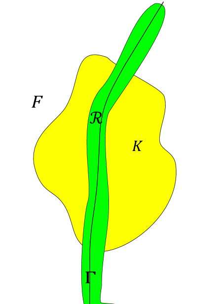
Figure 7.1: Schematic diagram showing $\Gamma$, $\mathcal{R}$, $K$ and $F$.

This setting describes a warp drive that appears from flat space and subsequently vanishes, returning to flat space. The interior of the warp drive is $\mathcal{R}$, and the openness of $\mathcal{R}$ ensures that the flat interior of the warp drive has finite size, and is not just a single point. $\mathcal{R}$ must contain a timelike geodesic in order to allow a free-falling observer to travel inside the flat interior. This is a very general conception of a warp drive, and in particular makes no assumptions about the existence of a special time coordinate where, for example, the lapse function is unity or spacelike hypersurfaces $\Sigma_{t}$ are intrinsically flat.

The compactness of the curved region $K$ may seem like an unnecessary and artificial restriction, given that many warp drives studied in the literature do not obey this constraint (for example, [1], [6], and [9]). However, if we imagine we are starting in a Riemann-flat universe and creating this warp drive, information of the warp drive’s existence should not be able to travel arbitrarily fast. The existence of curvature at arbitrary distances would imply that this information had travelled at arbitrarily high speeds.

7.2 Overview and intuition

We first give an overview of the arguments and results presented in this section, before giving their formal proofs. First of all, we argue that there exists an open sub-region $\tilde{\mathcal{R}}\subset\mathcal{R}$ that is isometric to a “cylinder” of flat spacetime, that is, one can choose a coordinate system $(\tau,x,y,z)$ in $\tilde{\mathcal{R}}$ such that $g_{\mu\nu}=\eta_{\mu\nu}$, with the boundary of a hypersurface of constant $\tau$ being a 2-sphere with constant spatial coordinates. The path $(\tau,\mathbf{0}),-\infty<\tau<\infty$ is $\Gamma$, so $\Gamma\subset\tilde{\mathcal{R}}$. These would be the local coordinates used by an observer on the geodesic $\Gamma$.

We then show that a time coordinate $t$ (which induces a normal vector field $\mathbf{n}=-\mathop{}\!\mathrm{d}t$) can be chosen on $F$ such that $t$ defines a reference frame. An observer following $\Gamma$ is at rest in this reference frame before entering $K$. Since $F$ extends to the section of $\Gamma$ beyond $K$, this gives us a well-defined and natural way to determine whether the observer exits $K$ with a different 4-velocity from the one they entered it with.

In Minkowski space, a spacelike hypersurface of zero extrinsic curvature gives rise to a constant normal vector $\mathbf{n}$, which is the 4-velocity of observers at rest in a frame that has this hypersurface as the set of points with $t=\text{constant}$. We call a time coordinate “locally Minkowskian” at a point $p$ if the neighbourhood of $p$ is Riemann-flat and the hypersurface $t=\text{constant}$ is extrinsically flat in a neighbourhood of $p$.

We next show that there exists an extension of $t$ inside $\tilde{\mathcal{R}}$ such that $t$ is locally Minkowskian everywhere in $\tilde{\mathcal{R}}$ too. Such a choice of $t$ gives a local frame of reference inside $\tilde{\mathcal{R}}$ and thus has useful intuitive value, as well as significance in relation to the freedom of choice of the lapse $N$, as we shall see. It also gives rise to a partial foliation of $M$, $\Sigma_{t^{*}}\equiv t^{-1}(t^{*})$ for $t^{*}\in\mathbb{R}$.

After choosing such a $t$, we show that at any point $p\in\tilde{\mathcal{R}}$, some $\tilde{x},\tilde{y},\tilde{z}$ can be chosen on an open set containing $p$ where the metric takes the following form:

$$\mathop{}\!\mathrm{d}s^{2}=-N^{2}\mathop{}\!\mathrm{d}t^{2}+\mathop{}\!\mathrm{d}\tilde{x}^{2}+\mathop{}\!\mathrm{d}\tilde{y}^{2}+\mathop{}\!\mathrm{d}\tilde{z}^{2}.$$

From this, we deduce that since $\tilde{\mathcal{R}}$ is flat, $N$ cannot be of a more general form than

$$N(t,\tilde{\mathbf{x}})=p(t)+\mathbf{q}(t)\cdot\tilde{\mathbf{x}},$$

for some $p$ and $\mathbf{q}$ depending only on time. This was in fact the original motivation for the ansatz (3.8). Lapses taking this form can be viewed as a uniform “acceleration of the time coordinate”, that is, the integral curve of $n^{\mu}$ would correspond to an accelerating observer. This means that the non-accelerating observers in the warp drive accelerate relative to the Eulerian observer following $n^{\mu}$. Since the vector $n^{\mu}$ is what we measure the net change in velocity of observers traversing $\tilde{\mathcal{R}}$ against, this corresponds to a rest frame transition. See Figure 7.3 for a visual depiction of this.

7.3 Formalism and proofs

7.3.1 Construction of $\tilde{\mathcal{R}}$

First, we prove the existence of $\tilde{\mathcal{R}}$ as described above. Take a point $p_{0}\in\Gamma$ in the causal past of $\Gamma\cap\partial K$ (i.e. before the observer enters the warp drive) and its timelike tangent vector along $\Gamma$, $\mathbf{n}_{0}\in T_{p_{0}}M$. Since $\mathcal{R}$ is simply connected and Riemann-flat, a coordinate system $(\tau,x,y,z):\mathcal{R}\rightarrow\mathbb{R}$ can be constructed such that associated tangent vector to the coordinate $\tau$ has the same components as $\mathbf{n}_{0}$, and that the metric takes the Minkowskian form. $\Gamma$ is the path $(\tau,\mathbf{0}),\tau\in\mathbb{R}$. Now define $\tilde{r}>0$ by

$$\tilde{r}^{2}\equiv\inf{\{x^{2}(q)+y^{2}(q)+z^{2}(q):q\in\partial\mathcal{R}\}}.$$ (7.1)

By openness of $\mathcal{R}$ and compactness of $K$, we must have $\tilde{r}>0$. Then we simply define

$$\tilde{\mathcal{R}}\equiv\{q\in\mathcal{R}:x^{2}(q)+y^{2}(q)+z^{2}(q)<\tilde{r}^{2}\},$$ (7.2)

and our construction is complete. $\tilde{\mathcal{R}}$ is a subset of $\mathcal{R}$, is clearly open as it is the preimage of an open set under a continuous mapping, and in these coordinates, it is manifest that $\tilde{\mathcal{R}}$ is isometric (not just homeomorphic like $\mathcal{R}$) to an infinitely-long, Riemann-flat 3+1 cylinder. $\Box$

7.3.2 Construction of the time coordinate and reference frame outside $K$

For a schematic diagram displaying the following decomposition of $M$, see Figure 7.2. A reference frame, in Minkowski space, can be determined from the choice of only one timelike vector at some point, and extending it by parallel transport to make a vector field $\mathbf{n}$ on the whole of Minkowski space. Since Minkowski space is flat and simply connected, this extension is unique. There will also exist a timelike coordinate $t$ that one can derive from this, satisfying $-\mathop{}\!\mathrm{d}t=\mathbf{n}$, with the minus sign a convention ensuring that $\mathbf{n}$ is future-pointing, that is, $n^{0}>0$.

To create a global reference frame on the flat region $F$, we can similarly take the tangent vector of $\Gamma$, $\mathbf{n}_{0}$, at $p_{0}$, and define a vector at another point $q\in F$ by parallel-transporting the vector at $p$ along a path contained in $F$. Since $F$ is Riemann-flat and simply connected, the resulting vector at $q$ is independent of the path chosen. Using this method, we can define a unique vector field

$$\mathbf{n}:p\in F\rightarrow T_{p}F.$$

This gives us a global reference frame on $F$, set to be at rest with respect to the observer following $\Gamma$ before entering $K$, which allows us to quantify the change in the observer’s 4-velocity after passing through $K$, thus determining whether a rest frame transition has occurred. Again, we can take a coordinate $t:F\rightarrow\mathbb{R}$ such that $-\mathop{}\!\mathrm{d}t=\mathbf{n}$, choosing $t$ such that

$$0=\inf{\{t(\tilde{\mathcal{R}}\cap K)\}},$$ (7.3)

and we define

$$T\equiv\sup{\{t(\tilde{\mathcal{R}}\cap K)\}}.$$ (7.4)

Finally, we choose some $\tilde{K}\supset K$ such that the intersection of $\tilde{\mathcal{R}}$ and $\partial\tilde{K}$ has $t(\tilde{\mathcal{R}}\cap\partial\tilde{K})=\{0,T\}$, that is, we extend $K$ to $\tilde{K}$ so that the boundary of the section of $\tilde{\mathcal{R}}$ contained in $\tilde{K}$ has $t=0$ at one end and $t=T$ at the other. We also de-specify $t$ on $\tilde{K}\setminus K$ so that we are free to choose $t$ as we like inside $\tilde{\mathcal{R}}\cap\tilde{K}$. $\tilde{\mathcal{R}}$ and $\tilde{K}$ will be the main regions we shall study from now on.

It is crucial that we do not extend $\mathbf{n}$ along a path inside $\mathcal{R}$, as the point of this analysis is to see how the 4-velocity of an observer following $\Gamma$ changes relative to the background reference frame defined by $\mathbf{n}$ in $F$. If we extended it along a path inside $\mathcal{R}$, we would ensure that the observer following $\Gamma$ remains at rest with respect to the local reference frame defined by $\mathbf{n}$, and the possible discontinuity in the normal vector field from extending $\mathbf{n}$ to $\mathcal{R}\cup F$ would instead occur in $F$.

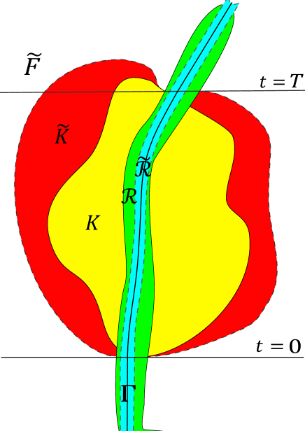
Figure 7.2: Schematic diagram showing $\Gamma$, $\mathcal{R}$, $\tilde{\mathcal{R}}$, $K$, $\tilde{K}$ and $\tilde{F}$. $\tilde{K}\supset K$ is such that the boundary $\partial\tilde{K}\cap\tilde{\mathcal{R}}$ is composed of two sections, one at $t=0$ and the other at $t=T$, the “entry” and “exit” of $\tilde{K}$.

7.3.3 Construction of the time coordinate inside $\tilde{\mathcal{R}}$

In $\tilde{F}\equiv M\setminus\tilde{K}$, the time coordinate is already specified. How may we choose it inside $\tilde{K}$, and in particular $\tilde{\mathcal{R}}\cap\tilde{K}$? One may imagine that since $\tilde{\mathcal{R}}$ is flat, one can analytically extend $t$ inside $\tilde{\mathcal{R}}\cap\tilde{K}$, to create a continuous time coordinate with a constant associated normal vector inside $\tilde{\mathcal{R}}$. However, this is not in general possible, a consequence of the flat region $\tilde{F}\cup\tilde{\mathcal{R}}$ not being simply connected. There is no guarantee that the parallel transport of $\mathbf{n}$ defined at some point with $t<0$ along a path traversing $\tilde{\mathcal{R}}$ will match $\mathbf{n}$ on the other side of $K$.

So what freedom do we have to choose $t$ inside $\tilde{\mathcal{R}}$? What is the most natural choice of $t$? If it were always possible to choose a time coordinate $t$ such that within $\tilde{\mathcal{R}}$ we have $N=N(t)$, this would imply that rest frame transitions are impossible, contrary to the example in Section 3. Therefore, we must search for something weaker. The next-best option is to have $\tilde{R}_{t}\equiv\tilde{\mathcal{R}}\cap\Sigma_{t}$ extrinsically flat (a locally-Minkowskian time coordinate), which in turn implies that it is also intrinsically flat by the Gauss equation. This is given in general as follows:

$$\tensor{\gamma}{{}_{\rho}^{\alpha}}\tensor{\gamma}{{}_{\sigma}^{\beta}}\tensor{\gamma}{{}_{\mu}^{\gamma}}\tensor{\gamma}{{}_{\nu}^{\delta}}\prescript{(4)}{}{R}_{\alpha\beta\gamma\delta}=\prescript{(3)}{}{R}_{\rho\sigma\mu\nu}+K_{\rho\mu}K_{\sigma\nu}-K_{\rho\nu}K_{\sigma\mu},$$ (7.5)

where $\gamma_{\mu\nu}=g_{\mu\nu}+n_{\mu}n_{\nu}$. Since the ambient space $\tilde{\mathcal{R}}$ is flat and the extrinsic curvature $K_{\mu\nu}$ is assumed to vanish, we are left with

$$\prescript{(3)}{}{R}_{\rho\sigma\mu\nu}=0.$$

We will now show that such a choice of $t$ always exists by explicit construction. Once such a $t$ has been chosen, we will be able to see exactly what the restrictions on the associated lapse $N$ are.

Take $p_{0}$ again and, using the same method with parallel transport, construct a vector field on $\tilde{\mathcal{R}}$ from the normal vector $\mathbf{n}$ at this point:

$$\mathbf{n}_{1}:p\in\tilde{\mathcal{R}}\rightarrow T_{p}\tilde{\mathcal{R}}.$$

In exactly the same way, choosing some point in $\Gamma$ after it has traversed $\tilde{K}$, we can construct a second vector field:

$$\mathbf{n}_{2}:p\in\tilde{\mathcal{R}}\rightarrow T_{p}\tilde{\mathcal{R}}.$$

These vector fields are the extension of the global reference frame on $\tilde{F}$ inside $\tilde{\mathcal{R}}$, with $\mathbf{n}_{1}$ from the past of $\tilde{K}$ and $\mathbf{n}_{2}$ from the future. As explained above, there is no reason that they must agree inside $\tilde{\mathcal{R}}$.

Now we reuse the Minkowskian coordinate system $(\tau,x,y,z)$ inside $\tilde{\mathcal{R}}$, choosing $\tau=0$ to coincide with $t=0$. In the coordinate basis we have $n_{1}^{\mu}=(1,\mathbf{0})$, and we now define $\bm{\sigma}$ such that

$$\begin{gathered}n_{2}^{\mu}=(\gamma,\gamma\bm{\sigma}),\\ \gamma\equiv(1-\sigma^{2})^{-\frac{1}{2}},\qquad\sigma\equiv|\bm{\sigma}|<1.\end{gathered}$$ (7.6)

$\bm{\sigma}$ is a constant vector, so $\mathop{}\!\mathrm{d}\bm{\sigma}=0$, where $\mathop{}\!\mathrm{d}$ denotes the exterior derivative. This implies $\exists\thinspace\phi:\tilde{\mathcal{R}}\rightarrow\mathbb{R}$ such that $\bm{\sigma}=\mathop{}\!\mathrm{d}\phi$. Looking at the expressions for $\mathbf{n}_{1},\mathbf{n}_{2}$ and $\bm{\sigma}$, we see

$$\mathbf{n}_{2}=\gamma(\mathbf{n}_{1}+\bm{\sigma})\iff\mathbf{n}_{2}=\gamma(-\mathop{}\!\mathrm{d}\tau+\mathop{}\!\mathrm{d}\phi),$$ (7.7)

a coordinate-independent equation. Now define

$$\tau_{0}\equiv\inf{\{\tau(p):p\in\tilde{\mathcal{R}}\cap t^{-1}(T)}\},$$

recalling that

$$\tilde{\mathcal{R}}\cap t^{-1}(T)\subset\partial\tilde{K},$$

that is, $\tilde{\mathcal{R}}\cap t^{-1}(T)$ is the “exit” of the compact region $\tilde{K}$ inside $\tilde{\mathcal{R}}$. $\phi$ is only specified up to an arbitrary constant, so we take it that $\phi=0$ somewhere in the boundary of $\tilde{R}_{T}$, with $\phi\geq 0$ inside $\tilde{R}_{T}$.

Consider the section of the hypersurface $t=T$ inside $\tilde{\mathcal{R}}$, the “exit” of $\tilde{K}$. This has a constant normal

$$(n_{2})_{\mu}=(-\gamma,\gamma\bm{\sigma}),$$

so using usual Euclidean geometry, it has the planar equation

$$-\tau+\bm{\sigma}\cdot\mathbf{x}=\text{constant}.$$ (7.8)

Thus we see that the infimum of $\tau$ on this surface, $\tau_{0}$, will be reached at the (limiting) point where $\bm{\sigma}\cdot\mathbf{x}$ is minimised. Since $\mathop{}\!\mathrm{d}\phi=\bm{\sigma}$, we can also see that

$$\phi=\phi_{0}+\bm{\sigma}\cdot\mathbf{x},$$ (7.9)

for some $\phi_{0}\in\mathbb{R}$. Therefore we see that minimising $\tau$ within the surface $t=T$ is equivalent to minimising $\phi$. Since we set $\phi$ such that its minimum on $\tilde{R}_{T}$ is zero, for any point where $\tau=\tau_{0}$ and $t=T$, $\phi=0$. Also, since hypersurfaces of constant $\tau$ have a fixed boundary in these coordinates (independent of $\tau$) and $\phi$ does not depend on $\tau$ either, this means $\phi\geq 0$ everywhere inside $\tilde{\mathcal{R}}$.

Now it is time to choose the time coordinate $t$ inside $\tilde{\mathcal{R}}$. There are many possible choices that give a valid time coordinate, continuous at $t=0$ and $t=T$ with $\tilde{R}_{t}$ being extrinsically flat, so here we give just one, to prove existence:

$$t=\frac{T}{\tan{\sigma}}\tan{\left(\frac{\sigma\tau}{\tau_{0}+\phi}\right)},$$ (7.10)

or if $\sigma=0$, we simply take

$$t=T\left(\frac{\tau}{\tau_{0}}\right),$$ (7.11)

as in that case $\phi\equiv 0$. See Figure 7.3 for a diagram showing this choice of $t$. This satisfies the necessary conditions:

1. $\tau=0\implies t=0$ and ($\tau=\tau_{0},\phi=0)\implies t=T$.

2. The hypersurfaces $\tilde{R}_{t}$ are extrinsically flat.

3. $t=T\implies-\mathop{}\!\mathrm{d}t$ is parallel to $\mathbf{n}_{2}$, and thus the normalised normal vector field associated to this choice of $t$ is continuous, and $t$ is a legitimate time coordinate.

The first of these points follows immediately from (7.10) and (7.11). The second can be seen by observing that a hypersurface in $\tilde{\mathcal{R}}$ with $t=\text{constant}$ is described by

$$\tau=k(\tau_{0}+\phi),$$ (7.12)

for some $k>0$. Since $\phi$ takes the form $\phi=\phi_{0}+\bm{\sigma}\cdot\mathbf{x}$, $\tilde{R}_{t}$ is isometric to a section of a 3-dimensional plane in Minkowski space, and clearly has no extrinsic curvature. The last point follows from calculating $-\mathop{}\!\mathrm{d}t$, and finding

$$-\mathop{}\!\mathrm{d}t\propto-(\tau_{0}+\phi)\mathop{}\!\mathrm{d}\tau+\tau\mathop{}\!\mathrm{d}\phi,$$

where the constant of proportionality is strictly positive. Using this and (7.7), the condition for $-\mathop{}\!\mathrm{d}t\propto\mathbf{n}_{2}$ is that $\tau_{0}+\phi=\tau$. But this is precisely the condition that $t=T$ in (7.10) and (7.11). Therefore, our time coordinate $t$ is continuous with a continuous, normalised, everywhere-timelike normal vector field $\mathbf{n}=-N\mathop{}\!\mathrm{d}t$, where $N:\tilde{F}\cup\tilde{\mathcal{R}}\rightarrow(0,\infty)$ is the associated lapse, and the construction of our time coordinate is complete. $\Box$

Figure 7.3: A choice of $t$ that is locally Minkowskian, in the region $\tilde{\mathcal{R}}\cap\tilde{K}$. The vector fields $\mathbf{n}_{1}$ and $\mathbf{n}_{2}$ have constant components throughout $\tilde{\mathcal{R}}$.

7.3.4 Construction of local coordinate system in $\tilde{\mathcal{R}}$

Now that we have vanishing extrinsic curvature of $\tilde{R}_{t}$, it is time to see what this means. Choose a $(x^{\prime},y^{\prime},z^{\prime})$ on $\tilde{\mathcal{R}}$ such that in the ADM formalism, its metric can be written as

$$\mathop{}\!\mathrm{d}s^{2}=-N^{2}\mathop{}\!\mathrm{d}t^{2}+\delta_{ij}(\mathop{}\!\mathrm{d}x^{\prime i}-\beta^{\prime i}\mathop{}\!\mathrm{d}t)(\mathop{}\!\mathrm{d}x^{\prime j}-\beta^{\prime j}\mathop{}\!\mathrm{d}t),$$ (7.13)

for some shift vector $\bm{\beta}^{\prime}$. This must be possible since the spatial slices are intrinsically flat, so we can take the induced metric to be $\delta_{ij}$. The extrinsic curvature tensor of a hypersurface $t=\text{constant}$ in this metric is, as proven in Appendix B,

$$K_{ij}=\frac{1}{N}\partial_{(i}\beta^{\prime}_{j)}.$$ (7.14)

Therefore, the vanishing of the extrinsic curvature implies that $\bm{\beta}^{\prime}$ is a Killing vector of the hypersurfaces. Now we apply the coordinate transformation

$$t\rightarrow t,$$

$$x^{\prime}\rightarrow\tilde{x}(t,x^{\prime},y^{\prime},z^{\prime}),$$

$$y^{\prime}\rightarrow\tilde{y}(t,x^{\prime},y^{\prime},z^{\prime}),$$

$$z^{\prime}\rightarrow\tilde{z}(t,x^{\prime},y^{\prime},z^{\prime}),$$

to some small open region inside $\tilde{\mathcal{R}}$, setting

$$\begin{gathered}(\partial_{t}\tilde{x},\partial_{t}\tilde{y},\partial_{t}\tilde{z})=\bm{\beta}^{\prime},\\ (\tilde{x}(t_{0},x^{\prime},y^{\prime},z^{\prime}),\tilde{y}(t_{0},x^{\prime},y^{\prime},z^{\prime}),\tilde{z}(t_{0},x^{\prime},y^{\prime},z^{\prime}))=(x^{\prime},y^{\prime},z^{\prime}),\end{gathered}$$ (7.15)

for some $0<t_{0}<T$. The region must be small in order to ensure that the integral curves of $\bm{\beta}^{\prime}$ do not go so far as to leave $\tilde{\mathcal{R}}$. However, since this argument can be applied to any part of $\mathcal{\tilde{R}}$, this is not problematic. One can calculate that this means the new metric $g_{\mu\nu}$ has $g_{0\mu}=(-N^{2},0,0,0)$. Without calculation, we also know that the spatial metric must be preserved, as we are shifting points along a Killing vector field of the hypersurfaces, under which the spatial metric is invariant.

Noting that since the time coordinate $t$ did not change, the lapse $N$ did not change either, we see that the metric now becomes

$$\mathop{}\!\mathrm{d}s^{2}=-N^{2}\mathop{}\!\mathrm{d}t^{2}+\mathop{}\!\mathrm{d}\tilde{x}^{2}+\mathop{}\!\mathrm{d}\tilde{y}^{2}+\mathop{}\!\mathrm{d}\tilde{z}^{2}.$$

Since here $K_{\mu\nu}=0$, one can see from the Ricci equation (4.26) that there is at least one component of the Riemann tensor proportional to $\partial_{i}\partial_{j}N$ for each pair $\{i,j\}\in\{1,2,3\}^{2}$. Requiring that $\mathcal{R}$ is flat therefore means that the most general form that the lapse may take in this coordinate system is linear in the spatial coordinates, giving

$$N(t,\tilde{\mathbf{x}})=p(t)+\mathbf{q}(t)\cdot\tilde{\mathbf{x}},$$

for some $p$, $\mathbf{q}$ dependent only on $t$. $\Box$

Looking at Figure 7.3, it is now clear exactly how rest frame transitions work geometrically. We simply have to choose a geometry inside $\tilde{\mathcal{R}}$ such that the extension of $\mathbf{n}$ inside $\tilde{\mathcal{R}}$ from the past and the future do not agree, differing by a vector characterised by $\bm{\sigma}$. Then free-falling observers will exit $\tilde{K}$ with a 3-velocity of $-\bm{\sigma}$.

8 Summary

In this paper we have identified, analysed, and solved a problem that, to our knowledge, plagues all warp drives previously studied. If, sometime in the far future, warp drives could actually be constructed and used for interstellar travel, then they would most likely need to perform some kind of rest frame transition, as we have described here. Otherwise, the object being carried by the warp bubble would need to be equipped with its own rockets, or other conventional forms of propulsion, in order to match velocities with the destination.

The concept of rest frame transition also gives stronger backing to the widely-accepted belief that superluminal travel allows for time travel. The object travelling superluminally must transition to the rest frame $S^{\prime}$, otherwise it cannot move back in time in $S$. To the best of our knowledge, this subtle issue has not been addressed so far in the literature. In this paper we have shown that this issue can be resolved using our new class of warp drives with rest frame transitions, and even provided, for the first time, an example of a double warp drive geometry that explicitly contains closed timelike geodesics.

We also demonstrated in this paper that weak energy condition violations arise in almost all (if not all) metrics of the general form

$$\mathop{}\!\mathrm{d}s^{2}=-N^{2}\mathop{}\!\mathrm{d}t^{2}+\delta_{ij}(\mathop{}\!\mathrm{d}x^{i}-\beta^{i}\mathop{}\!\mathrm{d}t)(\mathop{}\!\mathrm{d}x^{j}-\beta^{j}\mathop{}\!\mathrm{d}t),$$ (8.1)

with well-localised warp fields, whether or not we choose $N$ and $\bm{\beta}$ such that the spacetime is “warp-drive-like”, that is, contains a warp bubble. Furthermore, these violations occur whether or not the warp drive is superluminal. This suggests that the WEC violations arise not from any supposed deep connection between superluminal travel and negative energy, but rather from the particular form of the metric. Positive-energy warp drives may still be allowed within classical general relativity, but only if they could be formulated using a different type of metric.

Appendix A Calculations in the ADM formalism with the extrinsic curvature tensor

In this appendix, we give a brief discussion of the intricacies of performing calculations with the extrinsic curvature tensor $K_{\mu\nu}$, as an addendum to Sections 4.3 and 7.

One can express a general metric in the ADM formalism with induced hypersurface metric $\gamma_{ij}$, lapse $N$, and shift vector $\beta^{i}$ as

$$g_{\mu\nu} =\begin{pmatrix}-N^{2}+\beta^{k}\beta_{k}&-\beta_{j}\\ -\beta_{i}&\gamma_{ij}\end{pmatrix},$$ (A.1)

$$g^{\mu\nu} =\begin{pmatrix}-\frac{1}{N^{2}}&-\frac{1}{N^{2}}\beta^{j}\\ -\frac{1}{N^{2}}\beta^{i}&\gamma^{ij}-\frac{1}{N^{2}}\beta^{i}\beta^{j}\end{pmatrix},$$ (A.2)

where $\gamma^{ij}$ is the inverse of the induced metric and $\beta_{i}\equiv\gamma_{ij}\beta^{j}$. The normal vector $\mathbf{n}$ is once again given by

$$n_{\mu}=(-N,\mathbf{0}),\qquad n^{\mu}=\frac{1}{N}(1,\bm{\beta}),$$ (A.3)

and we define the projection operator

$$\gamma_{\mu\nu}\equiv g_{\mu\nu}+n_{\mu}n_{\nu}.$$

Note that $\beta^{\mu}=(0,\bm{\beta})$ is a “spatial” vector, i.e. it is orthogonal to the normal. In general, we call a tensor spatial if the contraction of any index with the normal vector (in appropriate vector or covector form) gives zero.

When contracting tensors with the extrinsic curvature tensor, one can in general ignore components corresponding to the normal (in our case timelike) direction, and rewrite expressions using the spatial metric $\gamma$. For example, $K_{\mu\rho}g^{\rho\sigma}Q_{\sigma\nu}$ can be written as $K_{\mu j}\gamma^{jk}Q_{k\nu}$. This is despite the fact that neither $K_{\mu 0}$ nor $Q_{0\nu}$ are necessarily zero. One might expect that these components would in some way contribute to the result of the contraction, but this is not the case. For example, take an arbitrary vector $q^{\mu}$. Then

$$K_{\mu\nu}q^{\nu} =K_{\mu\nu}g^{\nu\rho}q_{\rho}$$ (A.4)

$$=K_{\mu\nu}(\gamma^{\nu\rho}-n^{\nu}n^{\rho})q_{\rho}$$

$$=K_{\mu\nu}\gamma^{\nu\rho}q_{\rho}-0$$

$$=K_{\mu j}\gamma^{jk}q_{k},$$

where we have used the fact that $K_{\mu\nu}n^{\nu}=0$ and $\gamma^{\mu 0}=0$. Therefore, the value of $q_{0}$ does not affect this contraction. The same holds for contractions with higher-rank tensors.

However, care must be taken. To be precise, what we are really doing in the last line is considering the projection of $q^{\mu}$ onto our hypersurface, $\tilde{q}^{\mu}\equiv\tensor{\gamma}{{}_{\nu}^{\mu}}q^{\mu}$ (the “spatial” part of $q^{\mu}$), and using the fact that the induced metric $\gamma_{ij}$ is perfectly adequate for raising and lowering spatial indices of spatial vectors such as $\tilde{q}^{\mu}$. In general,

$$\tilde{q}_{i}=(\tensor{g}{{}_{i}^{\nu}}+n_{i}n^{\nu})q_{\nu}=q_{i},$$ (A.5)

since $n_{i}=0$, but

$$\tilde{q}^{i}=(\tensor{g}{{}_{\nu}^{i}}+n^{i}n_{\nu})q^{\nu}=q^{i}+n^{i}n_{\nu}q^{\nu}\neq q^{i}.$$ (A.6)

Therefore, the last line in (A.4) is correct, but if we had written $K_{\mu\nu}q^{\nu}=K_{\mu j}\tensor{\gamma}{{}_{k}^{j}}q^{k}$, it would not have been:

$$K_{\mu\nu}\tensor{\gamma}{{}_{\rho}^{\nu}}q^{\rho} =K_{\mu\nu}\cdot(0,-q^{0}\beta^{i}+q^{i})^{\nu}$$ (A.7)

$$=K_{\mu i}(-q^{0}\beta^{i}+q^{i})$$

$$\neq K_{\mu i}q^{i}=K_{\mu j}\tensor{\gamma}{{}_{k}^{j}}q^{k}.$$

Instead, we would have to use $\tilde{q}^{\mu}$ to make it work. Looking back at (A.4), it would have been incorrect to write

$$K_{\mu\nu}q^{\nu}=K_{\mu j}q^{j}.$$ (A.8)

Again, for this to work, $q^{\mu}$ must be spatial, or the spatial part of $q^{\mu}$ – that is, $\tilde{q}^{\mu}$ – must be used instead. The rewriting of, for example, $K_{\mu\nu}K^{\mu\nu}$ as $K_{jk}K^{jk}$ in Section 4.3 works only because the extrinsic curvature is itself a spatial tensor.

Appendix B Proofs of identities (2.5), (4.28) and (4.31)

First, we derive (2.5), using $n_{\mu}=-N\nabla_{\mu}t$:

$$n^{\nu}\nabla_{\nu}n_{\mu} =-n^{\nu}\nabla_{\nu}(N\nabla_{\mu}t)$$ (B.1)

$$=-n^{\nu}(\nabla_{\nu}N)(\nabla_{\mu}t)-Nn^{\nu}\nabla_{\nu}\nabla_{\mu}t$$

$$=\frac{1}{N}n_{\mu}\mathcal{L}_{\mathbf{n}}N-Nn^{\nu}\nabla_{\mu}\nabla_{\nu}t$$

$$=\frac{1}{N}n_{\mu}\mathcal{L}_{\mathbf{n}}N+Nn^{\nu}\nabla_{\mu}\left(\frac{1}{N}n_{\nu}\right)$$

$$=\frac{1}{N}n_{\mu}\mathcal{L}_{\mathbf{n}}N-N\nabla_{\mu}\left(\frac{1}{N}\right)-n^{\nu}\nabla_{\mu}n_{\nu}$$

$$=\frac{1}{N}(\nabla_{\mu}N+n_{\mu}\mathcal{L}_{\mathbf{n}}N).$$

In terms of components, this is

$$n^{\nu}\nabla_{\nu}n_{\mu}=\left(-\frac{1}{N}\beta^{i}\partial_{i}N,\frac{1}{N}\partial_{i}N\right),$$ (B.2)

and therefore we see that

$$\text{Integral curves of $n^{\mu}$ are geodesics}\iff\partial_{i}N=0.\qquad\Box$$ (B.3)

Next, we prove the identity (4.31)

$$\gamma^{\mu\nu}\mathcal{L}_{\mathbf{n}}K_{\mu\nu}=\mathcal{L}_{\mathbf{n}}K+2K_{\mu\nu}K^{\mu\nu},$$ (B.4)

which we used in Section 4.3. It holds for an arbitrary smooth hypersurface with unit normal vector $\mathbf{n}$, and the derivation is a straightforward application of the properties of the Lie derivative. First we note that, from the definition of $K_{\mu\nu}$ and the Lie derivative, we have

$$K_{\mu\nu} =\frac{1}{2}\mathcal{L}_{\mathbf{n}}\gamma_{\mu\nu}$$ (B.5)

$$=\frac{1}{2}\left(n^{\rho}\nabla_{\rho}\gamma_{\mu\nu}+(\nabla_{\mu}n^{\rho})\gamma_{\rho\nu}+(\nabla_{\nu}n^{\rho})\gamma_{\mu\rho}\right)$$

$$=\frac{1}{2}\left(n^{\rho}\nabla_{\rho}(n_{\mu}n_{\nu})+\nabla_{\mu}(n^{\rho}\gamma_{\rho\nu})-n^{\rho}\nabla_{\mu}\gamma_{\rho\nu}+\nabla_{\nu}(n^{\rho}\gamma_{\mu\rho})-n^{\rho}\nabla_{\nu}\gamma_{\mu\rho}\right)$$

$$=\frac{1}{2}\left(n^{\rho}\nabla_{\rho}(n_{\mu}n_{\nu})-n^{\rho}\nabla_{\mu}\gamma_{\rho\nu}-n^{\rho}\nabla_{\nu}\gamma_{\mu\rho}\right)$$

$$=\frac{1}{2}\left(n_{\mu}n^{\rho}\nabla_{\rho}n_{\nu}+n_{\nu}n^{\rho}\nabla_{\rho}n_{\mu}\right)+\nabla_{(\mu}n_{\nu)},$$

having used metric compatibility and the fact that

$$n^{\mu}n_{\mu}=-1\implies\nabla_{\rho}(n^{\mu}n_{\mu})=0$$

to simplify the last two terms in the penultimate line. One can similarly show that

$$\mathcal{L}_{\mathbf{n}}\gamma^{\mu\nu}=-2\nabla^{(\mu}n^{\nu)}.$$ (B.6)

Therefore

$$K^{\mu\nu}=\frac{1}{2}\left(n^{\mu}n^{\rho}\nabla_{\rho}n^{\nu}+n^{\nu}n^{\rho}\nabla_{\rho}n^{\mu}\right)-\frac{1}{2}\mathcal{L}_{\mathbf{n}}\gamma^{\mu\nu}.$$ (B.7)

The Lie derivative obeys the product rule, so

$$\gamma^{\mu\nu}\mathcal{L}_{\mathbf{n}}K_{\mu\nu}=\mathcal{L}_{\mathbf{n}}K-K_{\mu\nu}\mathcal{L}_{\mathbf{n}}\gamma^{\mu\nu},$$ (B.8)

where

$$K\equiv g^{\mu\nu}K_{\mu\nu}=\gamma^{\mu\nu}K_{\mu\nu}.$$

We then find using (B.7) that

$$K_{\mu\nu}\mathcal{L}_{\mathbf{n}}\gamma^{\mu\nu}=-2K_{\mu\nu}K^{\mu\nu},$$ (B.9)

and the identity follows. We recover the identity used in Section 4.3,

$$\gamma^{ij}\mathcal{L}_{\mathbf{n}}K_{ij}=\mathcal{L}_{\mathbf{n}}K+2K_{ij}K^{ij},$$ (B.10)

by the discussion in Appendix A, since $K_{\mu\nu}$ is a spatial tensor. $\Box$

Finally, we find the expression for the spatial components of the extrinsic curvature tensor $K_{ij}$, (4.28). In this case, $g_{ij}=\gamma_{ij}=\delta_{ij}$. We begin from the last line of (B.5):

$$K_{\mu\nu}=\frac{1}{2}\left(n_{\mu}n^{\rho}\nabla_{\rho}n_{\nu}+n_{\nu}n^{\rho}\nabla_{\rho}n_{\mu}\right)+\nabla_{(\mu}n_{\nu)}.$$ (B.11)

Now we replace $\mu\rightarrow i$, $\nu\rightarrow j$, and use $n_{i}=0$ to get

$$K_{ij}=\nabla_{(i}n_{j)}.$$ (B.12)

Then

$$K_{ij} =\partial_{(i}n_{j)}-\Gamma_{(ij)}^{\rho}n_{\rho}$$ (B.13)

$$=0+N\Gamma_{ij}^{0}$$

$$=\frac{1}{2}N\left(g^{00}(\partial_{i}g_{0j}+\partial_{j}g_{0i}-\partial_{0}g_{ij})+g^{0k}(\partial_{i}g_{kj}+\partial_{j}g_{ki}-\partial_{k}g_{ij})\right)$$

$$=\frac{1}{2}N\left(-\frac{1}{N^{2}}(\partial_{i}(-\beta_{j})+\partial_{j}(-\beta_{i})-\partial_{0}\delta_{ij})+(-\frac{1}{N^{2}}\beta^{k})(\partial_{i}\delta_{kj}+\partial_{j}\delta_{ki}-\partial_{k}\delta_{ij})\right)$$

$$=\frac{1}{2}\frac{1}{N}\left((\partial_{i}\beta_{j}+\partial_{j}\beta_{i})+0\right)$$

$$=\frac{1}{N}\partial_{(i}\beta_{j)},$$

where we have used the definition of the Christoffel symbol

$$\Gamma_{\mu\nu}^{\rho}=\frac{1}{2}g^{\rho\sigma}(\partial_{\mu}g_{\sigma\nu}+\partial_{\nu}g_{\sigma\mu}-\partial_{\sigma}g_{\mu\nu}).\qquad\Box$$ (B.14)

Appendix C Tables of symbols

Due to the large number of functions and quantities represented by different symbols throughout the paper, we provide a summary of the most important ones in this appendix for ease of reference.

General

The following symbols appear in more than one section, with very similar or identical meanings.

$u$	Speed of destination rest frame as measured in passenger’s initial rest frame
$\gamma_{u}$	Lorentz factor for speed $u$
$\Sigma_{t}$	Hypersurface of constant $t$
$\mathbf{n},n^{\mu}$	Future-pointing unit normal vector to $\Sigma_{t}$
$N$	Lapse function associated to $t$ such that $\mathbf{n}=-N\mathop{}\!\mathrm{d}t$
$\bm{\beta}$	Shift vector
$\gamma_{ij}$	Induced metric on hypersurface $\Sigma_{t}$
$\Gamma_{RFT}$	Inextendible timelike geodesic corresponding to a rest frame transition

Section 1: Introduction

$\zeta(t)$	Path in $z$ followed by Alcubierre drive
$v(t)$	Velocity of Alcubierre drive, given by $\partial_{t}\zeta(t)$
$f$	Shape function of Alcubierre drive
$\alpha(\tau)$	Worldline of Alcubierre drive centre, a geodesic parameterised by proper time

Section 2: Natário drives cannot perform rest frame transitions

$T_{flat}$

Time at which warp drive vanishes

Section 3: A warp drive allowing for a rest frame transition

$\mathbf{r}(t)$	Path followed by warp drive centre
$\mathbf{v}(t,\mathbf{x})$	Velocity vector field of warp drive; 3-velocity of warp drive’s passenger at $(t,\mathbf{r}(t))$
$s(t,\mathbf{x})$	Function appearing in definition of lapse $N$
$T_{1}$, $\tau_{1}$	Coordinate and proper time at which warp drive starts transition ($T_{1}=\tau_{1}$)
$T_{2}$, $\tau_{2}$	Coordinate and proper time at which warp drive finishes transition ($T_{2}\neq\tau_{2}$)
$a(t)$	Transition function for shift vector $\bm{\beta}$; decreases smoothly from $1$ to $0$ in $T_{1}<t<T_{2}$
$b(t)$	Transition function for lapse $N$; takes form of bump function between $T_{1}<0<T_{2}$
$\lambda(t)$	Function of $a$; analogous to Lorentz factor
$\chi_{1}(\tau)$	Parametrisation of first part of geodesic inside warp drive by proper time, before transition ($0\leq t<T_{1}$)
$\chi_{2}(\tau)$	Parametrisation of second part of geodesic inside warp drive by proper time, during transition ($T_{1}\leq t<T_{2}$)
$\chi(\tau)$	Parametrisation of combination of $\chi_{1}$ and $\chi_{2}$ by proper time; also a geodesic

Section 4: Making a closed timelike geodesic

Every symbol describing the outgoing warp drive has a counterpart with a circumflex. These are the corresponding symbols describing the returning warp drive in the CTC spacetime, $M_{CTC}$. There are two other changes:

1. The critical times, $t=0,T_{1},T_{2}$, now become $\hat{t}=\hat{T}_{0},\hat{T}_{1},\hat{T}_{2}$ respectively.

2. $\hat{\mathbf{v}}$ finishes such that the warp drive is at rest in $S$, so for $\hat{t}\geq\hat{T}_{1}$, $\hat{\mathbf{v}}=(0,0,-u)$.

$h_{\mu\nu},\hat{h}_{\mu\nu}$	Perturbations to Minkowski metric in outgoing and returning warp drives’ domains respectively
$T_{finish}$	Time when second warp drive returns, as measured in $S$
$\bar{v}^{z}$, $\hat{\bar{v}}^{z}$	Average speeds (taken as positive) of both warp drives along their respective $z$ axes in $S$ and $\hat{S}$ respectively
$C$	Section of $t$ axis between $t=T_{finish}$ and $t=0$, assuming $T_{finish}<0$
$\Gamma_{CTC}$	Union of outgoing and returning geodesics at warp bubble centre and $C$; itself a geodesic
$\epsilon,\hat{\epsilon}$	Amount of proper time elapsed since start of transition
$\prescript{(CTC)}{}{\tensor{R}{{}_{\rho\sigma\mu\nu}}}$	Riemann tensor on CTC spacetime
$\tensor{R}{{}_{\rho\sigma\mu\nu}},\tensor{\hat{R}}{{}_{\rho\sigma\mu\nu}}$	Riemann tensors within respective domains of warp drives
$\gamma_{\mu\nu},\hat{\gamma}_{\mu\nu}$	Projection operators for hypersurfaces $\Sigma_{t}$, $\hat{\Sigma}_{\hat{t}}$
$K_{\mu\nu},\hat{K}_{\mu\nu}$	Extrinsic curvature tensors for hypersurfaces $\Sigma_{t}$, $\hat{\Sigma}_{\hat{t}}$

Section 5: The weak energy condition with a non-unit lapse

$\rho$	Eulerian energy density
$\phi_{i}$	Momentum flux of energy-momentum tensor; $\phi_{i}=G_{ni}$
$\psi$	Primitive of $\bm{\beta}$ in the curl-free case; $\bm{\beta}=\nabla\psi$

Section 6: An example of a double warp drive spacetime with a geodesic CTC

$q$	Bump function with $0\leq q(x)\leq 1$, $\operatorname{supp}{q}=(0,1)$ and $\int_{0}^{1}q(x)\mathop{}\!\mathrm{d}x=1$; here chosen as $q(x)=140x^{3}(1-x)^{3}$ for $0<x<1$
$q^{(-1)}$	Primitive of $q$, a “smooth step function”; $q^{(-1)}(x)=0$ for $x\leq 0$, $q^{(-1)}(x)=1$ for $x\geq 1$
$q^{(-2)}$	Second primitive of $q$; $q^{(-2)}(x)=0$ for $x\leq 0$
$r_{1}$	Radius of flat region inside warp drives
$r_{2}$	Radius of warp drives as measured by external observers in their respective frames
$t_{1},\hat{t}_{1}$	Times at which warp drives change from acceleration to deceleration
$t_{2}$, $\hat{t}_{2}$	Actual finish times of transition, slightly less than $T_{2}$, $\hat{T}_{2}$, to avoid collision of warp drives
$\alpha$	Acceleration parameter
$\kappa$	Constant associated with the choice of $q$; $\kappa=q^{(-2)}(1)$
$\omega$	$T_{1}/T_{2}$, fraction of the outgoing journey spent before the transition starts; same for both outgoing and returning sections

Section 7: General analysis of rest frame transitions

$M$	Entire spacetime
$K$	Compact region outside which $M$ is Riemann-flat
$F$	Complement of $K$; Riemann-flat
$\mathcal{R}$	Flat interior of warp bubble
$\Gamma$	Inextendible timelike geodesic inside $\mathcal{R}$
$\tilde{\mathcal{R}}$	Subset of $\mathcal{R}$ isometric to infinite 3+1 cylinder with $\Gamma\subset\tilde{\mathcal{R}}$
$\tilde{R}_{t}$	Hypersurface inside $\tilde{\mathcal{R}}$ of time $t$
$T$	Time at which observer in warp drive exits $\tilde{K}$
$\tilde{K}$	Superset of $K$ such that $\tilde{\mathcal{R}}\cap\partial\tilde{K}$ is composed of two disjoint hypersurfaces, one at $t=0$ and one at $t=T$
$\tilde{F}$	Complement of $\tilde{K}$; Riemann-flat
$\mathbf{n}_{1}$	Extension of $\mathbf{n}$ inside $\tilde{\mathcal{R}}$ from past of $\tilde{K}\cap\tilde{\mathcal{R}}$
$\mathbf{n}_{2}$	Extension of $\mathbf{n}$ inside $\tilde{\mathcal{R}}$ from future of $\tilde{K}\cap\tilde{\mathcal{R}}$
$\bm{\sigma}$	Proportional to spatial part of $\mathbf{n}_{2}$, when viewed in $(\tau,x,y,z)$ coordinates
$\phi$	Primitive of $\bm{\sigma}$, i.e. $\mathop{}\!\mathrm{d}\phi=\bm{\sigma}$
$\tau_{0}$	Infimum of $\tau$ on surface $t=T$

References

- [1] Miguel Alcubierre. The warp drive: hyper-fast travel within general relativity. Classical and Quantum Gravity, 11(5):L73–L77, may 1994. arXiv:gr-qc/0009013, doi:10.1088/0264-9381/11/5/001.
- [2] Barak Shoshany. Lectures on Faster-than-Light Travel and Time Travel. SciPost Phys. Lect. Notes, 10, 2019. arXiv:1907.04178, doi:10.21468/SciPostPhysLectNotes.10.
- [3] Francisco S. N. Lobo, editor. Wormholes, Warp Drives and Energy Conditions. Springer International Publishing, 2017. doi:10.1007/978-3-319-55182-1.
- [4] Serguei Krasnikov. Back-in-Time and Faster-than-Light Travel in General Relativity. Springer International Publishing, 2018. doi:10.1007/978-3-319-72754-7.
- [5] Erik Curiel. A Primer on Energy Conditions. In Dennis Lehmkuhl, Gregor Schiemann, and Erhard Scholz, editors, Towards a Theory of Spacetime Theories, pages 43–104. Springer New York, New York, NY, 2017. arXiv:1405.0403, doi:10.1007/978-1-4939-3210-8_3.
- [6] Jessica Santiago, Sebastian Schuster, and Matt Visser. Generic warp drives violate the null energy condition. Physical Review D, 105(6), 2022. URL: https://doi.org/10.1103%2Fphysrevd.105.064038, doi:10.1103/physrevd.105.064038.
- [7] Chris Van Den Broeck. A ‘warp drive’ with more reasonable total energy requirements. Classical and Quantum Gravity, 16(12):3973–3979, 1999. URL: https://doi.org/10.1088%2F0264-9381%2F16%2F12%2F314, doi:10.1088/0264-9381/16/12/314.
- [8] Pedro F. González-Díaz. Warp drive space-time. Physical Review D, 62(4), 2000. URL: https://doi.org/10.1103%2Fphysrevd.62.044005, doi:10.1103/physrevd.62.044005.
- [9] José Natário. Warp drive with zero expansion. Classical and Quantum Gravity, 19(6):1157–1165, 2002. URL: https://doi.org/10.1088%2F0264-9381%2F19%2F6%2F308, doi:10.1088/0264-9381/19/6/308.
- [10] Allen E. Everett. Warp drive and causality. Phys. Rev. D, 53:7365–7368, 1996. URL: https://link.aps.org/doi/10.1103/PhysRevD.53.7365, doi:10.1103/PhysRevD.53.7365.
- [11] Francisco S. N. Lobo. Closed timelike curves and causality violation. 2010. URL: https://arxiv.org/abs/1008.1127, doi:10.48550/ARXIV.1008.1127.
- [12] Jacob Hauser and Barak Shoshany. Time Travel Paradoxes and Multiple Histories. Phys. Rev. D, 102, Sep 2020. arXiv:1911.11590, doi:10.1103/PhysRevD.102.064062.
- [13] Barak Shoshany and Jared Wogan. Wormhole Time Machines and Multiple Histories. Gen. Relativ. Gravit., 55(44), 2023. arXiv:2110.02448, doi:10.1007/s10714-023-03094-8.
- [14] Barak Shoshany and Zipora Stober. Time Travel Paradoxes and Entangled Timelines. 2023. arXiv:2303.07635, doi:10.48550/arXiv.2303.07635.
- [15] Erik W. Lentz. Breaking the warp barrier: Hyper-fast solitons in einstein-maxwell-plasma theory, 2020. URL: https://arxiv.org/abs/2006.07125, doi:10.48550/ARXIV.2006.07125.
- [16] Erik W. Lentz. Hyper-Fast Positive Energy Warp Drives. In 16th Marcel Grossmann Meeting on Recent Developments in Theoretical and Experimental General Relativity, Astrophysics and Relativistic Field Theories, 12 2021. arXiv:2201.00652.
- [17] Alexey Bobrick and Gianni Martire. Introducing physical warp drives. Classical and Quantum Gravity, 38(10):105009, 2021. URL: https://doi.org/10.1088%2F1361-6382%2Fabdf6e, doi:10.1088/1361-6382/abdf6e.
- [18] Shaun D B Fell and Lavinia Heisenberg. Positive energy warp drive from hidden geometric structures. Classical and Quantum Gravity, 38(15):155020, 2021. URL: https://doi.org/10.1088%2F1361-6382%2Fac0e47, doi:10.1088/1361-6382/ac0e47.
- [19] Ken D. Olum. Superluminal travel requires negative energies. Physical Review Letters, 81(17):3567–3570, 1998. URL: https://doi.org/10.1103%2Fphysrevlett.81.3567, doi:10.1103/physrevlett.81.3567.
- [20] Barak Shoshany. OGRe: An Object-Oriented General Relativity Package for Mathematica. Journal of Open Source Software, 6(65):3416, 2021. doi:10.21105/joss.03416.
- [21] Barak Shoshany and Jared Wogan. OGRePy: An Object-Oriented General Relativity Package for Python. In preparation.
- [22] Martin Bojowald. Hamiltonian formulation of general relativity, pages 17–112. Cambridge University Press, 2010. doi:10.1017/CBO9780511921759.003.