A Unifying Perspective on Non-Stationary Kernels for Deeper Gaussian Processes

Abstract

The Gaussian process (GP) is a popular statistical technique for stochastic function approximation and uncertainty quantification from data. GPs have been adopted into the realm of machine learning in the last two decades because of their superior prediction abilities, especially in data-sparse scenarios, and their inherent ability to provide robust uncertainty estimates. Even so, their performance highly depends on intricate customizations of the core methodology, which often leads to dissatisfaction among practitioners when standard setups and off-the-shelf software tools are being deployed. Arguably the most important building block of a GP is the kernel function which assumes the role of a covariance operator. Stationary kernels of the Matérn class are used in the vast majority of applied studies; poor prediction performance and unrealistic uncertainty quantification are often the consequences. Non-stationary kernels show improved performance but are rarely used due to their more complicated functional form and the associated effort and expertise needed to define and tune them optimally. In this perspective, we want to help ML practitioners make sense of some of the most common forms of non-stationarity for Gaussian processes. We show a variety of kernels in action using representative datasets, carefully study their properties, and compare their performances. Based on our findings, we propose a new kernel that combines some of the identified advantages of existing kernels.

1 Introduction

The Gaussian process (GP) is arguably the most popular member of the large family of stochastic processes and provides a powerful and flexible framework for stochastic function approximation in the form of Gaussian process regression (GPR) [Williams and Rasmussen(2006)]. A GP is characterized as a Gaussian probability distribution over (model or latent) function values $\{f(\mathbf{x}_{1}),f(\mathbf{x}_{2}),f(\mathbf{x}_{3}),...\}$ and therefore over the subspace $\{f:f(\mathbf{x})=\sum_{i}^{m}\leavevmode\nobreak\ \alpha_{i}k(\mathbf{x},\mathbf{x}_{i};h)\leavevmode\nobreak\ \forall\leavevmode\nobreak\ \mathbf{x}\in\mathcal{X},\leavevmode\nobreak\ m\in\mathbb{N},\leavevmode\nobreak\ \alpha_{i}\in\mathbb{R}\}$, called a reproducing kernel Hilbert space (RKHS), where $k(\mathbf{x},\mathbf{x}_{i};h)$ is the kernel function, $h\in\Theta$ is a vector of hyperparameters, and $\mathcal{X}$ is the input space. The RKHS — as the name would suggest — is directly influenced by the choice of the kernel function, which assumes the role of the covariance function in the GP framework. This double role makes the kernel an important building block when it comes to optimizing the flexibility, accuracy, and expressiveness of a GP.

In a recent review [Pilario et al.(2020)Pilario, Shafiee, Cao, Lao, and Yang], it was pointed out that the vast majority of applied studies using GPs employ the radial basis function (RBF) kernel (also referred to as the squared exponential or Gaussian kernel). The fraction is even higher when we include other stationary kernels. Stationary kernels are characterized by $k(\mathbf{x}_{i},\mathbf{x}_{j})=k(|\mathbf{x}_{i}-\mathbf{x}_{j}|)$, i.e., covariance matrix entries only depend on some distance between data points in the input domain, not on their respective location. Stationary kernels are popular because they carry little risk — in terms of model misspecification — and come with only a few hyperparameters that are easy to optimize or train. However, it has been shown that the stationarity assumption can lead to poor prediction performance and unrealistic uncertainty quantification that is affected mostly by point geometry [Noack and Reyes(2023)]. In other words, uncertainty will increase when moving away from data points at a constant rate across the input space. To overcome these limitations, significant research attention has been drawn to non-stationary Gaussian process regression sampson1992nonparametric,paciorek2003nonstationary,paciorek2006spatial. Non-stationary kernels depend on the respective locations in the input space explicitly, i.e., $k(\mathbf{x}_{i},\mathbf{x}_{j})\neq k(|\mathbf{x}_{i}-\mathbf{x}_{j}|)$. This makes them significantly more flexible and expressive leading to higher-quality estimates of uncertainty across the domain. Even so, non-stationary kernels are rarely used in applied machine learning (ML) due to the inherent difficulty of customization, optimizing hyperparameters, and the associated risks of model misspecification (wrong hyperparameters), overfitting, and computational costs due to the need to find many hyperparameters snoek2012practical, noack2023exact. When applied correctly, non-stationary GPs have been shown to provide significant advantages over their stationary counterparts, especially in scenarios where the data exhibit non-stationary behavior schabenberger2017statistical.

This paper aims to bring some structure to the use of non-stationary kernels and related techniques to make it more feasible for the practitioner to use these kernels effectively. Throughout this paper — in the hope of covering the most practical set of available options — we focus on and compare four ways to handle non-stationarity in a dataset:

1. Ignore it: Most datasets and underlying processes exhibit some level of non-stationarity which is often simply ignored. This leads to the use of stationary kernels of the form $k_{stat}=k(|\mathbf{x}_{i}-\mathbf{x}_{j}|)$; $|\cdot|$ is a norm appropriate to the properties of the input space. Given the key takeaways in [Pilario et al.(2020)Pilario, Shafiee, Cao, Lao, and Yang], this option is chosen by many which serves as the main motivation for the authors to write this perspective.

2. Parametric non-stationarity: Kernels of the form $k(\mathbf{x}_{i},\mathbf{x}_{j})=\sum_{d=1}^{N}g_{d}(\mathbf{x}_{i})g_{d}(\mathbf{x}_{j})k_{stat}(|\mathbf{x}_{i}-\mathbf{x}_{j}|)$, where $g_{d}(\mathbf{x})$ can be any parametric function over the input space and $N$ is some positive integer.

3. Deep kernels: Kernels of the form $k_{stat}(|\boldsymbol{\phi}(\mathbf{x}_{i})-\boldsymbol{\phi}(\mathbf{x}_{j})|)$, where $\boldsymbol{\phi}$ is a neural network, and $k_{stat}$ is any stationary kernel. This kernel was introduced by Wilson et al. [Wilson et al.(2016)Wilson, Hu, Salakhutdinov, and Xing] and was quickly established as a powerful technique, even though potential pitfalls related to overfitting were also discovered [Ober et al.(2021)Ober, Rasmussen, and van der Wilk].

4. Deep GPs: Achieving non-stationarity not by using a non-stationary kernel, but by stacking stationary GPs — meaning the output of one GP becomes the input to the next, similar to how neural networks are made up of stacked layers — which introduces a non-linear transformation of the input space and thereby non-stationarity [Damianou and Lawrence(2013)].

Non-stationarity can also be modeled through the prior-mean function of the Gaussian process but, for the purpose of this paper, we use a constant prior mean and focus on the four methods described above. From the brief explanations of the three types of non-stationarity, it is instantly clear that deriving, implementing, and deploying a non-stationary kernel and deep GPs (DGPs) can be an intimidating endeavor. The function $g_{d}$ (in #2 above), for instance, can be chosen to be any sum of local basis functions — linear, quadratic, cubic, piecewise constant, etc. — any polynomial or sums thereof, and splines, just to name a few. Given the vast variety of neural networks (in #3), choosing $\boldsymbol{\phi}$ is no easier. DGPs involve stacking GPs which increases flexibility but also leads to a very large number of hyperparameters, or latent variables, making optimization and inference a big challenge. In addition, a more complex kernel generally results in reduced interpretability — a highly valued property of GPs.

This paper is concerned with shining a light on the characteristics and performance of different kernels and experiencing them in action. In a very pragmatic approach, we study the performance of the three methodologies above to tackle non-stationarity and compare them to a stationary Matérn kernel to create a baseline. Our contributions can be summarized as follows:

1. We strategically choose a representative set of test kernels and investigate their properties.

2. We choose test datasets to study the performance of the chosen kernels.

3. We derive performance and (non)-stationarity metrics that allow fair comparisons of the non-stationary kernels and the selected deep GP implementation.

4. We compare the performance of the candidate kernels tasked with modeling the test datasets and present the uncensored results.

5. We use the gathered insights to draw some conclusions and suggest a new kernel design for further investigation.

We identify and exploit two primary pathways to achieve non-stationary properties: through the application of deep architectures — deep kernels of deep GPs — and the utilization of parametric non-stationary kernels. Our work delves into the role of parametric non-stationary kernels arguing that these kernels offer a similar behavior to a deep-kernel architecture without any direct notion of deepness, hinting at the possibility that deepness and flexibility are practically synonymous. This provides a valuable computational perspective to the broader dialogue surrounding deep architectures and non-stationarity, offering insights that may be instrumental in future research.

The remainder of this paper is organized as follows. The next section introduces some minimal but necessary theory. There, we also introduce some measures that will help us later when it comes to investigating the performance of different kernels. Then we give an overview of the relevant literature and some background. Subsequently, we introduce a range of different kernels and some test datasets, which positions the reader to see each kernel in action in different situations. We then discuss the key takeaways; we give some pointers toward improved kernel designs, make remarks about the connection between non-stationary kernels and multi-task learning, and conclude with a summary of the findings.

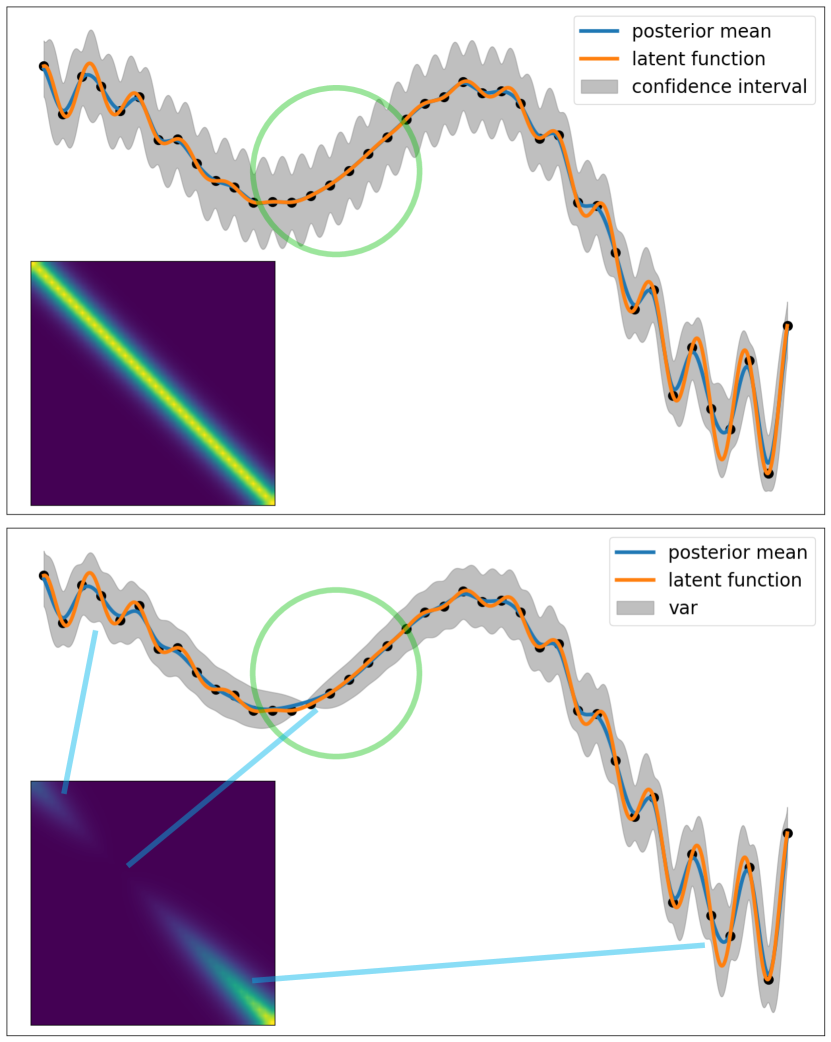
Figure 1: The key concept and essence of non-stationary kernels. A synthetic function — that is also later used for our computational experiments — was sampled at 40 equidistant points. The function is comprised of high-frequency regions (far left and right), and near-constant-gradient regions (center, green circle). A Gaussian process (GP) is tasked with interpolating the data using a stationary (top) and a non-stationary (bottom) kernel. For each case, the function approximation and the prior covariance matrix are presented. While the posterior mean is similar in both cases, the posterior variance differs substantially. Focusing on the central region, the uncertainty increases between data points, even though the function is very well-behaved there. The covariance matrix can deliver clues as to why this might happen. The matrix is constant along diagonals, which translates into uncertainties that depend on the distance from surrounding data points only, independent of where in the domain they are located. The non-stationary kernel has no such restriction and provides more realistic estimates of the uncertainty. The covariance entries are not constant along diagonals but correspond to different regions of the function (blue line connections).

2 Preliminaries

The purpose of this section is to give the reader the necessary tools to follow along with our computational experiments. It is not intended to be a complete or comprehensive overview of the GP theory or related methodologies. For the remainder of this paper, we consider some input space $\mathcal{X}\subset\mathbb{R}^{n}$ with elements $\mathbf{x}$. While we often think of the input space as a subspace of the Euclidean space, this is not a necessary assumption of the framework in general. We assume data $\mathcal{D}$ as a set of tuples $\{\mathbf{x}_{i},\mathbf{y}_{i}\}\leavevmode\nobreak\ \forall\leavevmode\nobreak\ i=\{1,2,3,...,|\mathcal{D}|\}$. In this work, except for a remark on multivariate GPs at the end, we will assume scalar $y_{i}$.

2.1 GPs in a Nutshell

The GP is a versatile statistical learning tool that can be applied to any black-box function. The ability of GPs to estimate both the mean and the variance of the latent function makes it an ideal ML tool for quantifying uncertainties in the function approximation. The prior Gaussian probability distribution is optimized or inferred, and then conditioned on the observational data $\mathcal{D}$ to yield a posterior probability density function (PDF). GPs assume a model of the form $y(\mathbf{x})\leavevmode\nobreak\ =\leavevmode\nobreak\ f(\mathbf{x})+\epsilon(\mathbf{x})$, where $f(\mathbf{x})$ is the unknown latent function, $y(\mathbf{x})$ is the noisy function evaluation (the measurement), $\epsilon(\mathbf{x})$ is the noise term, and $\mathbf{x}$ is an element of the input space $\mathcal{X}$. We define a prior over function values

$$p(\mathbf{f})=\frac{1}{\sqrt{(2\pi)^{|\mathcal{D}|}|\mathbf{K}|}}\exp\left[-\frac{1}{2}(\mathbf{f}-\mathbf{m})^{T}\mathbf{K}^{-1}(\mathbf{f}-\mathbf{m})\right],$$ (1)

where $\mathbf{K}$ is the covariance matrix defined by the kernel function $K_{ij}\leavevmode\nobreak\ =\leavevmode\nobreak\ k(\mathbf{x}_{i},\mathbf{x}_{j})$, and $\mathbf{m}$ is the prior mean obtained by evaluating the prior-mean function at points $\mathbf{x}_{i}$. We also define a likelihood $p(\mathbf{y}|\mathbf{f})$ which allows us to perform Bayesian inference, typically (but necessarily) using a multivariate Gaussian distribution

$$p(\mathbf{y}|\mathbf{f})=\frac{1}{\sqrt{(2\pi)^{|\mathcal{D}|}|\mathbf{V}|}}\exp\left[-\frac{1}{2}(\mathbf{y}-\mathbf{f})^{T}\mathbf{V}^{-1}(\mathbf{y}-\mathbf{f})\right],$$ (2)

where the covariance matrix $\mathbf{V}$ is used to describe measurement error arising from $\epsilon(\mathbf{x})$. Training the hyperparameters, extending the prior over latent function values at points of interest, marginalizing over $\mathbf{f}$, and conditioning on the data $\mathbf{y}$ yield the posterior PDF for the requested points [Williams and Rasmussen(2006)]. For example, for a Gaussian process with Gaussian likelihood, marginalization over $\mathbf{f}$ can be obtained in closed form

$$p(\mathbf{y}|h)=\int_{\mathcal{\mathbb{R}^{|\mathcal{D}|}}}p(\mathbf{y}|\mathbf{f})p(\mathbf{f})d\mathbf{f}=\frac{1}{\sqrt{(2\pi)^{|\mathcal{D}|}|\mathbf{K}+\mathbf{V}|}}\exp\left[-\frac{1}{2}(\mathbf{y}-\mathbf{m})^{T}(\mathbf{K}+\mathbf{V})^{-1}(\mathbf{y}-\mathbf{m})\right],$$ (3)

where we suppress the implicit conditioning on the hyperparameters. Training the GP is done by maximizing the log marginal likelihood — i.e., the log of Equation eq:margLik taken as a function of the hyperparameters $h$ when the data $\mathbf{y}$ is given —

$$\ln(p(\mathbf{y}|h))\propto-\frac{1}{2}(\mathbf{y}-\mathbf{m}(h))^{T}(\mathbf{K}(h)+\mathbf{V}(h))^{-1}(\mathbf{y}-\mathbf{m}(h))-\frac{1}{2}\ln(|\mathbf{K}(h)+\mathbf{V}(h)|)$$ (4)

with respect to the hyperparameters $h$. After the hyperparameters are found, the posterior is defined as p(f_0—y,h) &= ∫_R^—D— p(f_0—f,y,h) p(f—y,h) df
 ∝N(m_0 +κ^T  (K+V)^-1 (y-m ), K - κ^T (K+V)^-1 κ), where $\pmb{\kappa}=k(\mathbf{x}_{0},\mathbf{x}_{j})$, $\pmb{\mathcal{K}}=k(\mathbf{x}_{0},\mathbf{x}_{0})$, and $\mathbf{m}_{0}$ is the prior mean function evaluated at the prediction points $\mathbf{x}_{0}$. If, in a Bayesian setting, we want to further incorporate uncertainties in the hyperparameters $h\in\Theta$, Equation eq:pred_distr becomes p(f_0—y) &=  ∫_Θ p(f_0— y,h) p(h—y) dh, where $p(\mathbf{f}_{0}|\mathbf{y},h)$ is available in closed form eq:pred_distr. This basic framework can be extended by more flexible mean, noise, and kernel functions [Picheny and Ginsbourger(2013), Pilario et al.(2020)Pilario, Shafiee, Cao, Lao, and Yang, Noack and Sethian(2022), Noack and Sethian(2022), Noack et al.(2021)Noack, Zwart, Ushizima, Fukuto, Yager, Elbert, Murray, Stein, Doerk, Tsai, et al.].

2.2 The Covariance Operator of a GP: The Kernel or Covariance Function

In this work, the focus is on the kernel function — also called covariance function — of a GP, denoted $k:\mathcal{X}\times\mathcal{X}\rightarrow\mathbb{R}$. In the GP framework, the kernel function assumes the role of a covariance operator, i.e., the elements of the covariance matrix $\mathbf{K}$ in Equation eq:priorGP are defined by ${K}_{ij}=k(\mathbf{x}_{i},\mathbf{x}_{j})$. Because of that, kernel functions have to be symmetric and positive semi-definite (psd); a complete characterization of the class of valid kernel functions is given by Bochner’s theorem bochner1959lectures,adler1981geometry. At the same time, the kernel uniquely defines the underlying reproducing kernel Hilbert space (RKHS), which is the function or hypothesis space of the Gaussian process posterior mean.

Kernels are called “stationary” if the function only depends on the distance between the two inputs, not their respective locations, i.e., $k(\mathbf{x}_{i},\mathbf{x}_{j})=k(|\mathbf{x}_{i}-\mathbf{x}_{j}|)$. The arguably most prominent members are kernels of the Matérn class (see for instance [Stein(1999)]), which includes the exponential

$$k(\mathbf{x}_{i},\mathbf{x}_{j})=\sigma_{s}e^{-0.5\frac{||\mathbf{x}_{i}-\mathbf{x}_{2}||_{2}}{l}}$$ (5)

and the squared exponential (RBF) kernel

$$k(\mathbf{x}_{i},\mathbf{x}_{j})=\sigma_{s}e^{-0.5\frac{||\mathbf{x}_{i}-\mathbf{x}_{2}||_{2}^{2}}{l^{2}}},$$ (6)

the by-far most used kernel by practitioners [Pilario et al.(2020)Pilario, Shafiee, Cao, Lao, and Yang]; here, $||\cdot||_{2}$ is the Euclidean norm, which makes the kernel function both stationary and isotropic. These two special cases of the Matérn kernel class have two hyperparameters: $\sigma_{s}$, the signal variance, and $l$, the length scale, both of which are constant scalars applied to the entire domain $\mathcal{X}$. Stationary and isotropic kernels can be advanced by allowing anisotropy in the norm, i.e., $((\mathbf{x}_{i}-\mathbf{x}_{j})^{T}\mathbf{M}(\mathbf{x}_{i}-\mathbf{x}_{j}))^{1/2}$ where $\mathbf{M}$ is some symmetric positive definite matrix whose entries are typically included in the vector of hyperparameters that need to be found. Incorporating anisotropy allows the kernel function to stretch distances such that the implied covariances have ellipsoidal patterns (as opposed to spherical patterns for isotropic kernels). When $\mathbf{M}=\frac{1}{l}\mathbf{I}_{n}$ the isotropic kernels in Equations eq:expK and eq:rbfK are recovered; more generally, when $\mathbf{M}$ is diagonal with different elements along the diagonal, automatic relevance detection is recovered [Wipf and Nagarajan(2007)]. Other stationary kernel designs include the spectral kernel, the periodic kernel, and the rational quadratic kernel.

Non-stationary kernels do not have the restriction of only depending on the distance between the input points, but depend on their explicit positions $\mathbf{x}_{i}$ and $\mathbf{x}_{j}$, i.e., $k(\mathbf{x}_{i},\mathbf{x}_{j})\neq k(|\mathbf{x}_{i}-\mathbf{x}_{j}|)$. Formulating new non-stationary kernels comes with the difficulty of proving positive semi-definiteness which is often challenging. However, the statistics and machine learning literature has a variety of general approaches for applying valid non-stationary kernels; this is the primary topic of this paper which is discussed in Section 3. For now, it is important to keep in mind that the essence of stationary versus non-stationary kernels — due to the way they deal with the locations in the input space — manifests itself in the covariance matrix which, in the stationary case, has to be constant along all bands parallel to the diagonal for sorted and equidistant input points, a property that is not observed in the non-stationary case (see Figure 1). Therefore, non-stationary kernels lead to more descriptive, expressive, and flexible encodings of covariances and therefore uncertainties. Of course, in addition, the function space (the RKHS) contains a much broader class of functions as well when non-stationary kernels are used.

2.3 A Note on Scalability

Computational complexity is a significant challenge for GPs, for both stationary and non-stationary kernels. The need to calculate the log-determinant of and invert the covariance matrix — or solve a linear system instead — results in computational complexity of $\mathcal{O}(|\mathcal{D}|^{3})$, where $|\mathcal{D}|$ is the number of data points williams2006gaussian,luo2022sparse. This complexity limits the application of GPs for large-scale datasets. Several methods have been proposed to overcome this issue. Sparse methods snelson2005sparse,luo2022sparse and scalable GPR approaches hensman2015scalable have been developed for stationary GPs. For non-stationary GPs, methods such as local GPs gramacy2015local and the Bayesian treed GP gramacy2008bayesian have been proposed to tackle this issue. These methods have an origin in divide-and-conquer methods attempting to break down the problem into smaller, manageable pieces that can be solved independently hrluo_2022e, thereby reducing the computational complexity for each piece. However, these approaches can lead to a loss of global information, so finding the right balance between computational efficiency and model accuracy remains a key challenge. A recent approach can scale GPs to millions of data points without using approximations by allowing a compactly supported, non-stationary kernel to discover naturally occurring sparsity [Noack et al.(2023)Noack, Krishnan, Risser, and Reyes].

3 Non-Stationary Kernels

Stationary kernels are widely used primarily because they are easy and convenient to implement, even though the implied assumption of translation-invariant covariances is almost never exactly true for real-world data sets. As mentioned in Section 2, there are serious challenges associated with both deriving non-stationary kernels and choosing an appropriate and practical non-stationary kernel from the valid options for any given implementation of a Gaussian process. We now provide a brief overview of the literature on non-stationary kernels, including both a historical perspective of early developments followed by greater detail on three modern frameworks for non-stationary kernels as well as metrics for quantifying non-stationarity in data sets.

3.1 Historical Perspective

It has now been over three decades since the first paper on non-stationary kernels via “deformations” or warping of the input space appeared sampson1992nonparametric. Since then, the statistics literature has developed a number of approaches for non-stationary kernels, mostly in the context of modeling spatially-referenced data. These methods can broadly be categorized as basis function expansions and kernel convolutions, in addition to the aforementioned deformation approach. We now briefly summarize each method, focusing on aspects that apply directly to kernel functions for Gaussian processes.

The fundamental idea underpinning the deformation or warping approach sampson1992nonparametric is that instead of deriving new classes of non-stationary kernels one can keep isotropic kernels but obtain non-stationarity implicitly by rescaling interpoint distances in a systematic way over the input space. In other words, this approach transforms $\mathcal{X}$ to a new domain, say $\mathcal{X}^{*}$, wherein stationarity holds. The transformation, say $\boldsymbol{\phi}:\mathbb{R}^{n}\rightarrow\mathbb{R}^{n^{*}}$, is a (possibly nonlinear) mapping applied to elements of $\mathcal{X}$ to yield a non-stationary kernel via

$$k(\mathbf{x}_{i},\mathbf{x}_{j})=k_{stat}(||\boldsymbol{\phi}(\mathbf{x}_{i})-\boldsymbol{\phi}(\mathbf{x}_{j})||),$$ (7)

where $k_{stat}$ is an arbitrary stationary kernel function. Two extensions were later proposed to this approach damian2001bayesian,schmidt2003bayesian that supposed the mapping $\boldsymbol{\phi}(\cdot)$ was itself a stochastic process. For example, [Schmidt and O’Hagan(2003)] placed a Gaussian process prior on $\boldsymbol{\phi}(\cdot)$ — essentially coming up with the idea of deep kernels more than a decade before related ideas appeared in the machine learning literature. In some cases $n^{*}>n$, i.e., the mapping involves dimension expansion [Bornn et al.(2012)Bornn, Shaddick, and Zidek]. Ultimately, early approaches to warping the input space were largely unused due to a lack of computational tools for optimizing the mapping function $\boldsymbol{\phi}(\cdot)$ in a reliable and robust manner.

In contrast to deformations, basis function expansion methods provide constructive approaches for developing non-stationary kernel functions. The main idea for this approach arises from the Karhunen-Loève Expansion karhunen1946spektraltheorie,loeve1955probability of a (mean-zero) stochastic process in terms of orthogonal eigenfunctions $E_{m}(\cdot)$ and weights $w_{m}$:

$$f(\mathbf{x})=\sum_{m=1}^{\infty}w_{m}\hskip 1.50696ptE_{m}(\mathbf{x}).$$ (8)

This framework defines a Gaussian process if the weights have a Gaussian distribution; the implied kernel function is

$$k(\mathbf{x}_{i},\mathbf{x}_{j})=\sum_{m=1}^{\infty}{v_{m}}E_{m}(\mathbf{x}_{i})E_{m}(\mathbf{x}_{j}),$$

where the eigenfunctions and weight variances $v_{m}$ come from the Fredholm integral equation

$$\int_{\mathcal{X}}k(\mathbf{x}_{i},\mathbf{x}_{j})E_{m}(\mathbf{x}_{i})d\mathbf{x}_{i}=w_{m}E_{m}(\mathbf{x}_{j}).$$ (9)

If the infinite series in Equation 8 is truncated to the leading $M$ terms, the finite sum approximation to the kernel can be used instead and is optimal in the sense that it minimizes the variance of the truncation error for all sets of $M$ basis functions when the $E_{m}(\cdot)$ are the exact solutions to the Fredholm equation wikleChapter. The main task is then to model the weight-eigenfunction pairs $\{w_{m},E_{m}(\cdot)\}$, which can be done empirically using singular value decomposition holland or parametrically using, e.g., wavelets nychka2002.

Like basis function expansions, the kernel convolution approach is useful in that it provides a constructive approach to specifying both stochastic models and their covariance functions. The main result is that a stochastic process can be defined by the kernel convolution

$$f(\mathbf{x})=\int_{\mathcal{X}}\kappa_{\mathbf{x}}(\mathbf{u})dW({\bf u})$$ (10)

thiebaux76,thiebaux_pedder, where $W(\cdot)$ is a $n$-dimensional stochastic process and $\kappa_{\mathbf{x}}(\cdot)$ is a kernel function that depends on input location $\mathbf{x}$. [Higdon(2002)] summarizes the extremely flexible class of stochastic models defined using Equation kernelconvolution: see, for example, [Barry and Ver Hoef(1996)], [Ickstadt and Wolpert(1998)], and [Ver Hoef et al.(2004)Ver Hoef, Cressie, and Barry]. The popularity of this approach is due largely to the fact that it is much easier to specify (possibly parametric) kernel functions than a covariance function directly since the kernel functions only require $\int_{\mathbb{R}^{d}}\kappa_{\mathbf{x}}({\bf u})d{\bf u}<\infty$ and $\int_{\mathbb{R}^{d}}\kappa^{2}_{\mathbf{x}}({\bf u})d{\bf u}<\infty$. The process $f(\cdot)$ in Equation 10 is a Gaussian process when $W(\cdot)$ is chosen to be Gaussian, and the associated covariance function is

$$k(\mathbf{x}_{i},\mathbf{x}_{j})=\int_{\mathcal{X}}\kappa_{\mathbf{x}_{i}}(\mathbf{u})\kappa_{\mathbf{x}_{j}}(\mathbf{u})d{\bf u},$$ (11)

which cannot be written in terms of $||\mathbf{x}_{i}-\mathbf{x}_{j}||$ and is hence non-stationary. Various choices can be made for using this general framework in practice: replace the integral in Equation kernelconvolution with a discrete sum approximation Higdon98 or choose specific $\kappa_{\mathbf{x}}(\cdot)$ such that the integral in Equation eq:cov_kc can be evaluated in closed form Higdon99. The latter choice can be generalized to yield a closed-form kernel function that allows all aspects of the resulting covariances to be input-dependent: the length-scale paciorek2003nonstationary,paciorek2006spatial, the signal variance risser2015regression, and even the differentiability of realizations from the resulting stochastic process when the Matérn kernel is leveraged stein2005. This approach is often referred to as “parametric” non-stationarity since a non-stationary kernel function is obtained by allowing its hyperparameters to depend on input location. In practice, some care needs to be taken to ensure that the kernel function is not too flexible and can be accurately optimized paciorek2006spatial,anderes2008. We return to a version of this approach in the next section.

In conclusion, the statistics literature contains a broad set of techniques (only some of which are summarized here) for developing non-stationary kernel functions. However, historically speaking, these techniques were not widely adopted because, in most of the cases described here, the number of hyperparameters is on the same order as the number of data points. This property makes it very difficult to apply the kernels to real-world data sets due to the complex algorithms required to fit or optimize such models.

Nonetheless, the potential benefits of applying non-stationary kernels far outweigh the risks in our opinion, and this perspective is all about managing this trade-off. To do so, we now introduce three modern approaches to handle non-stationarity in datasets in order to later test them and compare their performance (Section 4).

3.2 Non-Stationarity via a Parametric Signal Variance

This class of non-stationary kernels uses a parametric function as the signal variance. The term $g(\mathbf{x}_{1})g(\mathbf{x}_{2})$ is always symmetric and psd [Noack and Sethian(2022)] and is, therefore, a valid kernel function. Also, any product of kernels is a valid kernel, which gives rise to kernels of the form

$$k(\mathbf{x}_{i},\mathbf{x}_{j})=g(\mathbf{x}_{i})g(\mathbf{x}_{j})k_{stat}(\mathbf{x}_{i},\mathbf{x}_{j}).$$ (12)

This can be seen as a special case of the non-stationary kernel derived in [Paciorek and Schervish(2006)] and [Risser and Calder(2015)] wherein the length-scale is taken to be a constant. [Risser and Calder(2015)], in particular, consider parametric signal variance and (anisotropic) length scale. In an extension of eq:nonpara1, any sum of kernels is a valid kernel which allows us to write

$$k(\mathbf{x}_{i},\mathbf{x}_{j})=\sum_{l=1}^{N}g_{l}(\mathbf{x}_{i})g_{l}(\mathbf{x}_{j})k_{stat}(\mathbf{x}_{i},\mathbf{x}_{j}).$$ (13)

The function $g$ can be any function defined on the input domain, but we will restrict ourselves to functions of the form

$$g(\mathbf{x})=\sum_{k=1}^{N_{2}}c_{k}\beta(\mathbf{x}_{k},\mathbf{x}),$$ (14)

where $c_{k}$ are some coefficients (or parameters), and $\beta(\mathbf{x}_{k},\mathbf{x})$ are basis functions centered at $\mathbf{x}_{k}$. For our computational experiments, we use radial basis functions of the form

$$\beta(\mathbf{x}_{k},\mathbf{x})=e^{-\frac{||\mathbf{x}_{k}-\mathbf{x}||^{2}}{w}},$$ (15)

where $w$ is the width parameter.

3.3 Deep Kernels

Algorithm 1 Deep Kernel with Neural Network

Input Set of points as arrays $x_{1}$, $x_{2}$, Hyperparameters $h\in\Theta$

Output Deep kernel covariance matrix of shape ($len(x_{1})\times len(x_{2})$)

Step 1: Define the neural network architecture with input dimension $n$, hidden layers, and appropriate activation functions

Step 2: Initialize or set the weights and biases of the neural network using $h$

Step 3: Transform $x_{1}$ and $x_{2}$ through the neural network

• Apply the forward pass of the neural network to all points in sets $x_{1}$ and $x_{2}$

• Store the transformed values as $x_{1nn}$ and $x_{2nn}$

Step 4: Calculate the pairwise distance matrix between $x_{1nn}$ and $x_{2nn}$

Step 5: Compute the deep kernel value using the distance matrix

• Apply a kernel function (e.g., exponential) to the distance matrix

• Scale and combine with other kernel functions if needed

Step 6: Return the deep kernel value

Our version of parametric non-stationarity operates on the signal variance only. This is by design so that we can separate the effects of the different kernels later in our tests. This next approach uses a constant signal variance but warps the input space to yield flexible non-constant length scales. The set of valid kernels is closed under non-linear transformation of the input space as long as this transformation is constant across the domain and the resulting space is considered a linear space. This motivates the definition of kernels of the form

$$k(\mathbf{x}_{i},\mathbf{x}_{j})=k_{stat}(||\boldsymbol{\phi}(\mathbf{x}_{i})-\boldsymbol{\phi}(\mathbf{x}_{j})||_{2}),$$ (16)

where $\boldsymbol{\phi}:\mathbb{R}^{n}\rightarrow\mathbb{R}^{n^{*}}$ can again be any scalar or vector function on the input space. Deep neural networks have been established as a preferred choice for $\boldsymbol{\phi}$ due to their flexible approximation properties which gives rise to, so-called, deep kernels (see Algorithm 1 for an implementation example). For our tests, we define a 2-deep-layer network with varying layer widths. While it is possible through deep kernels to perform dimensionality reduction, in this work we map the original input space into a linear space of the same dimensionality, i.e., $n=n^{*}$. Care must be taken not to use neural networks whose weights and biases, given the dataset set size, are underdetermined. That is why comparatively small networks are commonly preferred. We use ReLu as an activation function. The neural network weights and biases are treated as hyperparameters and are trained accordingly. We set $k_{stat}$ in eq:deepkernel to be the Matérn with $\nu=3/2$.

Our deep kernel construction shares the perspective of using a neural network to estimate a warping function sampson1992nonparametric. In [Zammit-Mangion et al.(2022)Zammit-Mangion, Ng, Vu, and Filippone], the authors propose an approach of deep compositional spatial models that differs from traditional warping methods in that it models an injective warping function through a composition of multiple elemental injective functions in a deep-learning framework. This allows for greater flexibility in capturing non-stationary and anisotropic spatial data and is able to provide better predictions and uncertainty quantification than other deep stochastic models of similar complexity. This uncertainty quantification is point-wise, similar to the deep GPs we introduced next.

3.4 Deep GPs

Deep Gaussian process (DGP) models are hierarchical extensions of Gaussian processes where GP layers are stacked — similar to a neural network — enhancing modeling flexibility and accuracy damianou2013deep,dunlop2018deep,jones2023alignment (more details can be found in the Appendix LABEL:app:deepGP). The DGP model is one of the deep hierarchical models [Ranganath et al.(2014)Ranganath, Tang, Charlin, and Blei, Salakhutdinov and Larochelle(2010), Teh et al.(2004)Teh, Jordan, Beal, and Blei] and consists of a number of variational Gaussian process layers defined by a mean function and a stationary covariance (kernel) function. The first layer uses constant zero means for lower-dimensional representation of the input data. The second layer uses constant zero means and takes the first layer’s output, generating the final model output. Each layer’s forward method applies the mean and covariance functions to input data and returns a multivariate normal distribution. This output serves as the next layer’s input. An additional method allows for the implementation of concatenation-based skip connections. We can impose more than two hidden layers for a single DGP according to our needs. However, we match the 2-layer structure used in our deep kernel and point out that the complexity of the neural architecture may not always lead to better performance.

Although each layer of DGP is equipped with stationary kernels, the output of one GP layer becomes the input to the next GP layer, hence the final output will not be stationary. For a DGP with $L$ layers, we can represent the model as follows:

f^(1)(x)∼GP(m^(1)(x),k^(1)(x,x’))
f^(2)(x)∼GP(m^(2)(f^(1)(x)),k^(2)(f^(1)(x),f^(1)(x’)))
⋯
f^(L)(x)∼GP(m^(L)(f^(L-1)(x)),k^(L)(f^(L-1)(x),f^(L-1)(x’))) Then, an optimizer and the variational Evidence Lower Bound (ELBO) are used for training of the DGP model. Using a variational approximation in ELBO, instead of exact inference, leads to manageable computational complexity of deeper GP models titsias2010bayesian. The deep Gaussian Processes (GPs) can be perceived as hierarchical models whose kernel does not admit a closed form. Crucially, this “hierarchy of means” is constructed via the means of the layer-distributions in the deep GP, but not higher moments like [Allenby and Rossi(2006), Daniels and Kass(1999), Mohamed(2015)]. Only the mean functions at each layer of the deep GP are contingent upon computations from preceeding layers, signifying hierarchies that rely on the first-order structure at every layer of the model.

Using a slightly different framework based on the Vecchia approximation, [Jimenez and Katzfuss(2023)] introduced a “deep Vecchia ensemble,” a hybrid method combining Gaussian processes (GPs) and deep neural networks (DNNs) for regression. This model builds an ensemble of GPs on DNN hidden layers, utilizing Vecchia approximations for GP scalability. Mathematically, the joint distribution of variables is decomposed using Vecchia’s approximation, and predictions are combined using a generalized product of experts. This approach offers both representation learning and uncertainty quantification. As described in the last section, a GP model can utilize a deep kernel, constructively combining the neural network’s (NN) and the GP’s strength, leading to a model that benefits from the GP’s interpretability and the NN’s flexibility wilson2016deep.

Our Bayesian DGP architecture follows [Sauer et al.(2022)Sauer, Cooper, and Gramacy] and includes a two-layer neural network, applied as a transformation to the input data. The first layer uses a rectified linear unit (ReLU) activation function and the second employs a sigmoid activation. This non-linear feature mapping expresses complex input space patterns (See Appendix LABEL:sec:appB).

Contrasting DGPs with deep-kernel GPs, DGPs use multiple GP layers to capture intricate dependencies, whereas deep-kernel GPs employ a NN for input data transformation before GP application. Essentially, while DGPs exploit GP layering to manage complex dependencies, deep kernel learning leverages NNs for non-linear input data transformation, enhancing the GP’s high-dimensional function representation ability.

3.5 Measuring Non-Stationarity of Datasets

When it comes to characterizing non-stationarity, some methods focus on non-stationarity in the mean function (e.g., polynomial regression), while others concentrate on the non-stationarity in the variance (e.g., geographically weighted regression fotheringham2003geographically). Non-stationarity is typically characterized by a change in statistical properties over the input space, e.g., changes in the dataset’s mean, variance, or other higher moments. Quantifying non-stationarity is an active area of research and in this paper, we merely introduce a particular kind of non-stationarity measure for the purpose of judging our test kernels when applied to the test datasets without claiming to propose a new method to measure it. Overall, measuring a given dataset’s non-stationarity properties is an important ingredient in understanding the performance of a particular kernel. For the reader’s convenience, we offer our non-stationarity measure as a pseudocode (see Algorithm 2). For theoretical motivation of the non-stationarity measure we use int this work, please refer to A.

To avoid bias through user-based subset selection we draw the location and width of a uniform distribution over the domain $[0,1]^{n}$ with dimensionality $n$. We then draw data points randomly from this distribution 100 times and use MCMC to get a distribution for the length scale and the signal variance in each iteration. The distribution of the means of the distributions of signal variances and length scales is then assessed to measure non-stationarity (See Algorithm 2).

Algorithm 2 Measuring non-stationarity via local, stationary-GP hyperparameter distributions.

1:procedure MeasureNonStationarity($\mathbf{X}$, $\mathbf{y},m$)$\triangleright$ $\mathbf{X}$ is the set of data points, $\mathbf{y}$ is the collected data, $m$ is the number of iterations

2:     length scale list = []

3:     signal variance list

4:     for i in $0$ to $m$ do

5:         $mean\sim U([0,1])$

6:         $standard\leavevmode\nobreak\ dev\sim U((0,1])$ $\triangleright$ alternatively draw size of subdomain.

7:         draw $m$ test data points:

8:         $\mathbf{X}_{t}\sim\mathcal{N}(mean,standard\leavevmode\nobreak\ dev)$ $\triangleright$ alternatively draw from uniform distr. over subdomain

9:         Find associated $\mathbf{y}_{t}$ in dataset

10:         initialize a stationary GP

11:         mean signal variance, mean length scale = run_mcmc()

12:         append new mean signal variance to signal variance list

13:         append new mean length scale to length scale list

14:     end for

15:     return signal variance list, length scale list

16:end procedure

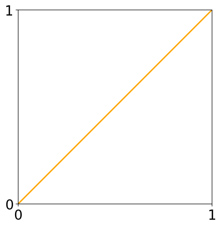
[b]0.3 [b]0.3 [b]0.3

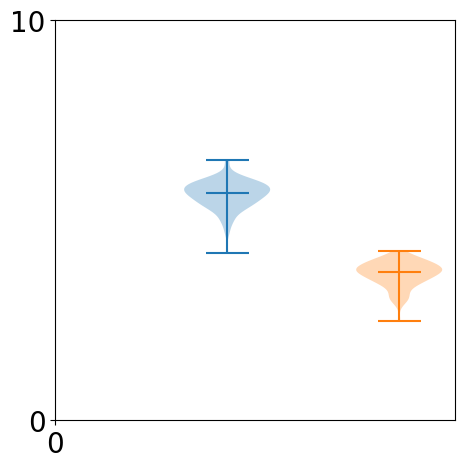
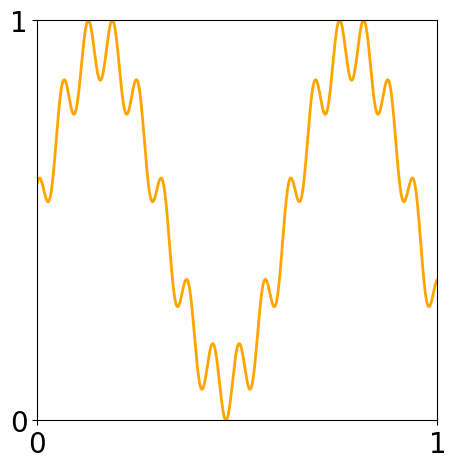
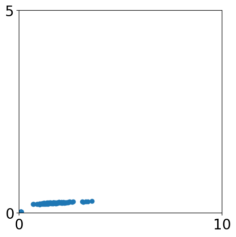
[b]0.3 [b]0.3 [b]0.3

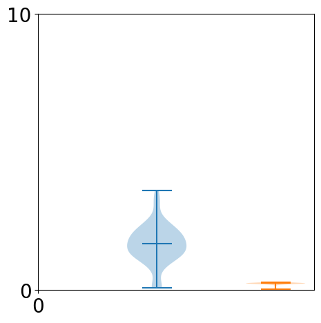
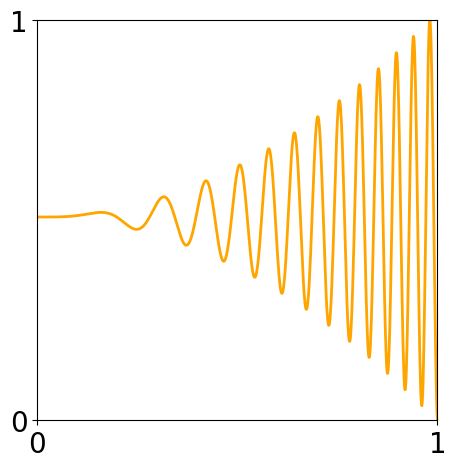
[b]0.3 [b]0.3 [b]0.3

Figure 2: A way of measuring the non-stationarity of a dataset or a synthetic function. When data is drawn randomly and a GP using a stationary kernel is trained via MCMC repeatedly, the distribution of the mean of the hyperparameters — here signal variance and isotropic length scale — can be used to measure non-stationarity. The stationary function (top) leads to a narrow distribution of the length scale and the signal variance. For the non-stationary function (bottom), the distribution for both hyperparameters is broader.

To test our non-stationary measure, we applied it to three synthetic functions (see Figure 2). In the first scenario (first row in Figure 2), where the signal is purely linear, the algorithm’s behavior leads to a high concentration of points in a single compact cluster when plotting the estimated length scale versus the signal variance. This concentration reflects the inherent stationarity of a linear signal, where the statistical properties do not change over the input space. The unimodal and concentrated distributions of both the estimated parameters in the violin plots further corroborate this observation. The consistency in the length scale and signal variance across multiple iterations of MCMC indicates that the underlying data structure is stationary. This case demonstrates the effectiveness of the proposed non-stationary measure in detecting the stationary nature of a linear signal.

In the second case (second row in Figure 2), the signal is a trigonometric curve with local oscillations. The algorithm’s response to this signal structure results in a single cluster when plotting the estimated length scale versus the signal variance but with a highly linear correlation. This linear correlation suggests a consistent relationship between the length scale and signal variance across different local oscillations. The unimodal concentrated distributions in the violin plots, coupled with a smaller variance in the estimated length scale, reflect a degree of stationarity within the local oscillations. The algorithm’s ability to capture this nuanced behavior underscores its sensitivity to variations in non-stationarity, even within a seemingly stationary pattern.

The third scenario (third row in Figure 2) presents a more complex signal structure, a trigonometric curve with varying amplitude and frequency. The algorithm’s reaction to this non-stationary signal is manifested in the clustering of points into two less concentrated clusters when plotting the estimated length scale versus the signal variance. This bimodal behavior in the clustering, as well as in the violin plots for both estimated parameters, reveals the underlying non-stationarity in the data. The varying magnitude of the signal introduces changes in statistical properties over space, leading to a broader distribution of the hyperparameters. The algorithm’s ability to discern this complex non-stationary pattern and reflect it in the clustering and distribution of the estimated hyperparameters illustrates its robustness and adaptability in measuring non-stationarity across diverse data structures.

The three cases in Figure 2 demonstrate the algorithm’s capability to measure non-stationarity through the local, stationary GP-hyperparameter distributions. The varying behaviors in clustering and distribution of the estimated parameters across the three cases provide insights into the underlying stationarity or non-stationarity of the signals. The algorithm’s sensitivity to these variations underscores its potential as a valuable tool for understanding and characterizing non-stationarity in different contexts.

3.6 Performance Measures

Throughout our computational experiments, we will measure the performance via three different error metrics as a function of training time. We argue that this allows us to compare methodologies across different implementations as long as all tests are run on the same computing architecture with similar hardware utilization. As for error metrics, we utilize the log marginal likelihood (Equation 4), the root mean square error (RMSE), and the Continuous Ranked Probability Score (CRPS). The RMSE is defined as

$$RMSE=\sqrt{\frac{\sum_{i}^{N}(y_{i}-f^{i}_{0})^{2}}{N}},$$ (17)

where $y_{i}$ are the data values of the test dataset and $f^{i}_{0}$ are the posterior mean predictions. The RMSE metric provides a measure of how closely the model’s predictions align with the actual values — approaching zero as fit quality improves — while the log marginal likelihood evaluates the fit of the Gaussian Process model given the observed data. The log marginal likelihood will increase as the model fits the data more accurately. The CRPS is defined as

$$CRPS(f_{0},y_{i})=\sigma\big{(}\frac{1}{\sqrt{\pi}}-2\psi(\frac{x-\mu}{\sigma})-\frac{x-\mu}{\sigma}(2\Psi(\frac{x-\mu}{\sigma}-1))\big{)},$$ (18)

where $\psi$ is the probability density function of a standard normal distribution and $\Psi$ is the associated cumulative distribution function. For a GP, $f_{0}$ is Gaussian with mean $\mu$ and variance $\sigma^{2}$. The CRPS is negative and approaches zero as fit quality improves. The CRPS is arguably the more important score compared to the RMSE because it is uncertainty aware. In other words, if the prediction accuracy is low, but sincerity in those regions is high — the algorithm is aware of its inaccuracy — the score improves.

Computational cost is becoming a main research topic in recent studies in large-scale non-parametric models hrluo_2022e,Scott2016cmcmc,hensman2015scalable, especially GPs litvinenko2019likelihood,geoga2020scalable,lin2023sampling,luo2022sparse. In our analysis, we sought to examine the progression of the optimization process. To achieve this, we established a callback function during the optimization phase, tracking the RMSE, the log marginal likelihood, and the CRPS as a function of compute time. In terms of interpretation, ideally, we expect the RMSE and the CRPS to decrease over time, suggesting that the model’s predictive accuracy and estimation of uncertainties are improving. On the other hand, the log marginal likelihood should increase, indicating a better fit of the model to the observed data. This analysis gives us a summary of the model’s learning process and helps us understand the progression of the optimization, thus providing valuable insights into the efficacy of our model and the optimization strategy employed.

4 Computational Experiments

The purpose of this section is to see how different kernels and a deep GP deal with non-stationarity in several datasets and to compare the characteristics and properties of the solutions. To make this comparison fair and easier, we ran all tests on the same Intel i9 CPU (Intel Core i9-9900KF CPU $@$ 3.60GHz $\times$ 8) and used the total compute time as the cost. As a performance metric, we calculate and observe the RMSE (Root Mean Squared Error, Equation 17), the CRPS (continuous rank probability score, Equation 18) of the prediction, and the log marginal likelihood of the observational data (Equation 2). We attempted to run fair tests in good faith; this means, the effort spent to set up each kernel or methodology was roughly proportional to a method’s perceived complexity, within reasonable bounds, similar to the effort expended by an ML practitioner — this meant minutes of effort for stationary kernels and hours to days for non-stationary kernels and DGPs. The optimizer to reach the final model was scipy’s differential evolution. We used an in-house MCMC (Markov Chain Monte Carlo) algorithm to create the plots showing the evolution of the performance metrics over time. In cases when our efforts did not lead to satisfactory performance, we chose to present the result “as is” to give the reader the ability to judge for themselves. To further the hands-on aspect of this section, we also included the used algorithms in the Appendix and on a specifically designed website together with links to download the data. The performance-measure-over-time plots were created without considering deep GPs due to incompatible differences in the implementations (see Section LABEL:app:deepGP). All computational experiments were run multiple times to make sure we showed representative results.

This section, first, introduces three datasets we use later to evaluate the performance of the test methodologies. Second, we present the unredacted, uncensored results of the test runs. The purpose is not to judge some kernels or methodologies as better or worse universally, but to evaluate how these techniques perform when tested under certain well-defined conditions and under the described constraints. We encourage the reader to follow our tests, to rerun them if desired, and to judge the performance of the methods for themselves.

4.1 Introducing the Test Datasets

We will consider three test data sets. All datasets are normalized such that the range and the image — the set of all measured function values — are in $[0,1]$.

For the first dataset, we define a one-dimensional synthetic function

$$f(x)=(\sin(5x)+\cos(10x)+(2(x-0.4)^{2})\cos(100x)+2.597)/3.94$$ (19)

data is drawn from. 50 data points are drawn randomly and the noise $\epsilon\sim\mathcal{N}(0,0.001)$ is added. Figure 3 presents the function and its non-stationary measures.

[b]

[b]0.45 [b]0.45

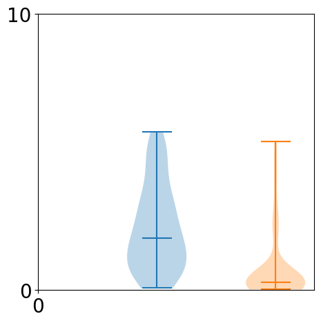
Figure 3: Test dataset 1 and its non-stationarity measures visualized as distributions in the hyperparameters of a stationary kernel trained on local subsets of that data. The dataset is derived from a one-dimensional synthetic function (see Equation eq:synthfunc). Non-stationarity appears to be present in the length scale and the signal variance.

Second, we consider a three-dimensional climate dataset that is available online (https://www.ncei.noaa.gov/data/global-historical-climatology-network-daily/),

consisting of in situ measurements of daily maximum surface air temperature (^∘C) collected from weather stations across the contiguous United States (geospatial locations defined by longitude and latitude) over time (the third dimension). The data and its non-stationarity measures are presented in Figure 4.

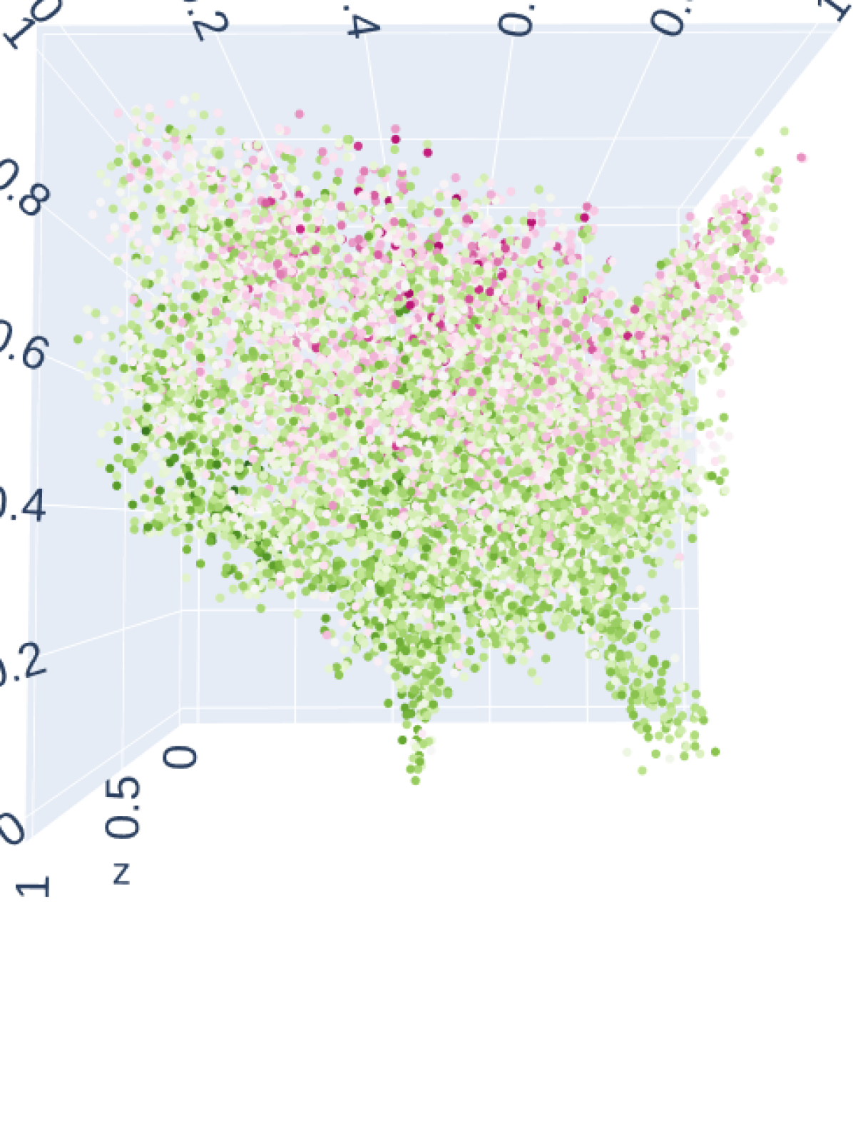
[b]0.45 [b]0.45

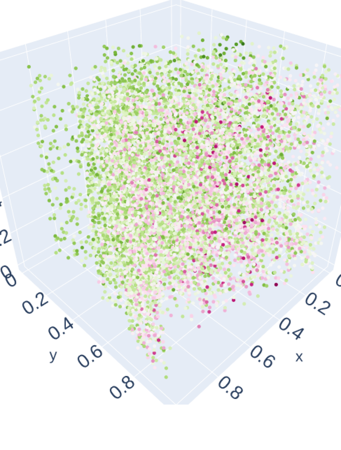
[b]0.45 [b]0.45

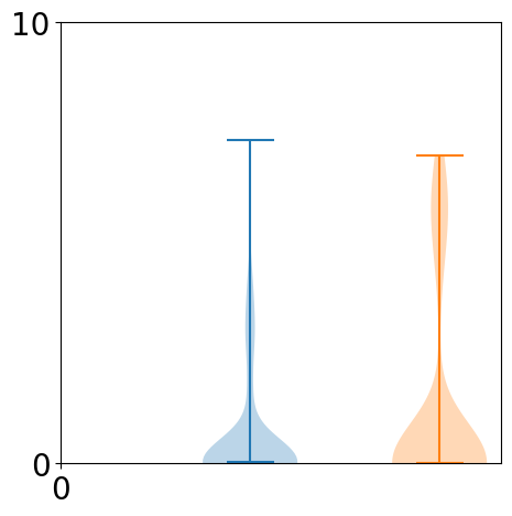
Figure 4: Test dataset 2 and its non-stationarity measures visualized as distributions in the hyperparameters of a stationary kernel trained on local subsets of that data. The dataset consists of recorded temperatures across the United States and a period of time. Weak non-stationarity appears to be present in the length scale and the signal variance.

Third, we consider a dataset that was collected during an X-ray scattering experiment at the CMS beamline at NSLSII, Brookhaven National Laboratory. The dataset originated from an autonomous exploration of multidimensional material state-spaces underlying the self-assembly of copolymer mixtures. Because the scientific outcome of this experiment has not been published yet, all scientific insights have been obscured by normalization and the removal of units. The dataset is presented in Figure 5.

[t]0.8

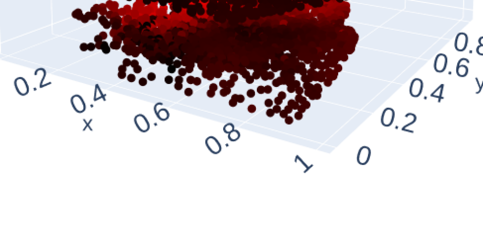
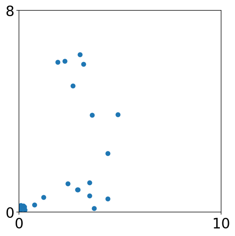
[b]0.45 [b]0.45

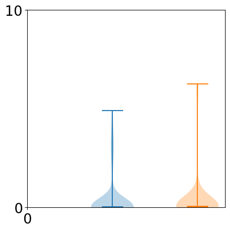
Figure 5: Test dataset 3 and its non-stationarity measures visualized as distributions in the hyperparameters of a stationary kernel trained on local subsets of that data. The dataset consists of analyzed X-ray scattering signals over $[0,1]^{3}$. Non-stationarity appears to be very weak but existent in both length scale and signal variance.

4.2 Results

In this section, we present quantitative results of how the different kernels and deep GPs performed when tasked to learn the underlying data-generating latent functions that produced the test datasets introduced in the previous section. For each test, we show the model and its uncertainties across the domain or a subdomain after convergence of a global evolutionary optimization of the log marginal likelihood, and the performance measures as a function of the compute time of an MCMC algorithm. Code snippets can be found in the Appendix and on our website (see the Code Availability paragraph at the end). To reiterate, for all tests, we put ourselves in the position of an ML practitioner setting up each algorithm under a reasonable-effort constraint — we did not optimize each method to its full extent because this would not lead to a fair comparison. However, we used our best judgment and followed online documentation closely. The same thought process was put into the exact design of the kernels; of course, one could always argue that a particular model would have performed better using more hyperparameters. For the fairness of the comparison, we kept the number of hyperparameters similar across the kernels for a particular computational experiment and increased the number of kernel parameters in a near-proportional fashion for the non-stationary kernels as we moved to higher dimensions. See Table 1 for the number of hyperparameters for the different experiments. All non-stationary kernels were implemented in the open-source GP package fvGP (https://github.com/lbl-camera/fvGP). We tried two different deep GPs, the gpflux package (https://github.com/secondmind-labs/GPflux) and the Bayesian deep GP (BDGP) by [Sauer et al.(2022)Sauer, Cooper, and Gramacy, Sauer et al.(2023)Sauer, Cooper, and Gramacy] (https://cran.r-project.org/web/packages/deepgp/index.html). We selected the latter in its two-layer version for our final comparisons because of performance issues with the gpflux package (see Figure 7).

Table 1: Number of hyperparameters for our computational experiments.

	Number of hyperparameters per experiment
Kernel functions	1D Synthetic	3D Climate	3D X-ray
Stationary, $k_{stat}$	2	3	3
Parametric non-stationary, $k_{para}$	15	58	58
Deep kernel, $k_{nn}$	48	186	186

4.2.1 One-Dimensional Synthetic Function

Our one-dimensional synthetic test function was introduced in Section 4.1. The stationary reference kernel ($k_{stat}$) is a Matérn kernel with $\nu=3/2$

$$k_{stat}(x_{i},x_{j})=\sigma^{2}\left(1+\frac{\sqrt{3}d}{l}\right)\exp\left(-\frac{\sqrt{3}d}{l}\right),$$ (20)

where $l$ is the length scale, and $d=||x_{i}-x_{j}||_{2}=|x_{i}-x_{j}|$. The parametric non-stationary kernel in this experiment was defined as

$$k_{para}(x_{i},x_{j})=\big{(}g_{1}(x_{i})g_{1}(x_{j})+g_{2}(x_{i})g_{2}(x_{j})\big{)}k_{stat},$$ (21)

where

$$g_{a}(x)=\sum_{b=1}^{6}c^{b}_{a}\exp{[-0.5(||\Tilde{x}_{b}-x||^{2})/w_{a}]},$$ (22)

$\Tilde{x}=\{0,0.2,0.4,0.6,0.8,1\}$, leading to a total of 15 hyperparameters — counting two $g_{a}$ functions in the sum, a constant width of the radial basis functions for each $g_{a}$, and a constant length scale. The deep kernel

$$k_{nn}(x_{i},x_{j})=k_{stat}(\phi(x_{i}),\phi(x_{j})),$$ (23)

where $\phi$ is a fully connected neural network mapping $\mathbb{R}\rightarrow\mathbb{R}$, with ReLu activation functions and two hidden layers of width five, which led to a total of 48 hyperparameters (weights, biases, and one constant signal variance). The results, presented in Figure 6, show a gradual improvement in approximation performance as more flexible kernels are used. The stationary kernel ($k_{stat}$) stands out through its fast computation time. However, the keen observer notices similar uncertainties independent of local properties of the latent function; only point spacing is considered in the uncertainty estimate. That is in stark contrast to the parametric non-stationary kernel ($k_{para}$) and the deep kernel ($k_{nn}$) which both predict lower uncertainties in the well-behaved center region of the domain. This is a very desirable characteristic of non-stationary kernels. The deep kernel and parametric non-stationary kernel reached very similar approximation performance but the deep kernel was by far the most costly to train. The BDGP predicts a very smooth model with subpar accuracy compared to the other methods. We repeated the experiment with different values for the nugget, and let the algorithm choose the nugget, without further success. This is not to say the method cannot perform better, but we remind the reader that we are working under the assumption of reasonable effort, which, in this case, was insufficient to reach a better performance. We share the code with the reader in the Appendix (see LABEL:sec:appB) for reproducibility purposes. The MCMC sampling runs revealed what was expected, the stationary kernel converges most robustly; however, all kernels led to a stable convergence within a reasonable compute time.

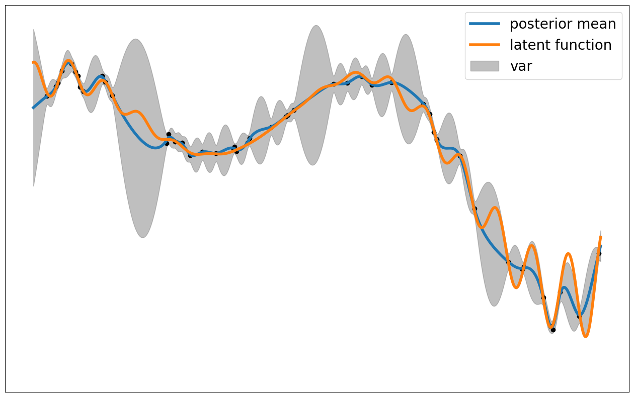
[b]0.45 [b]0.45

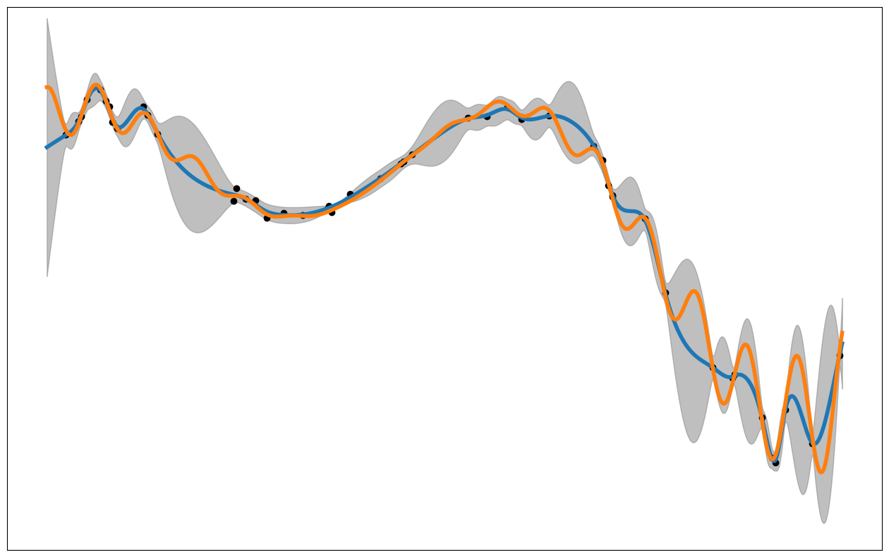
[b]0.45 [b]0.45

[b]0.8

[b]0.8

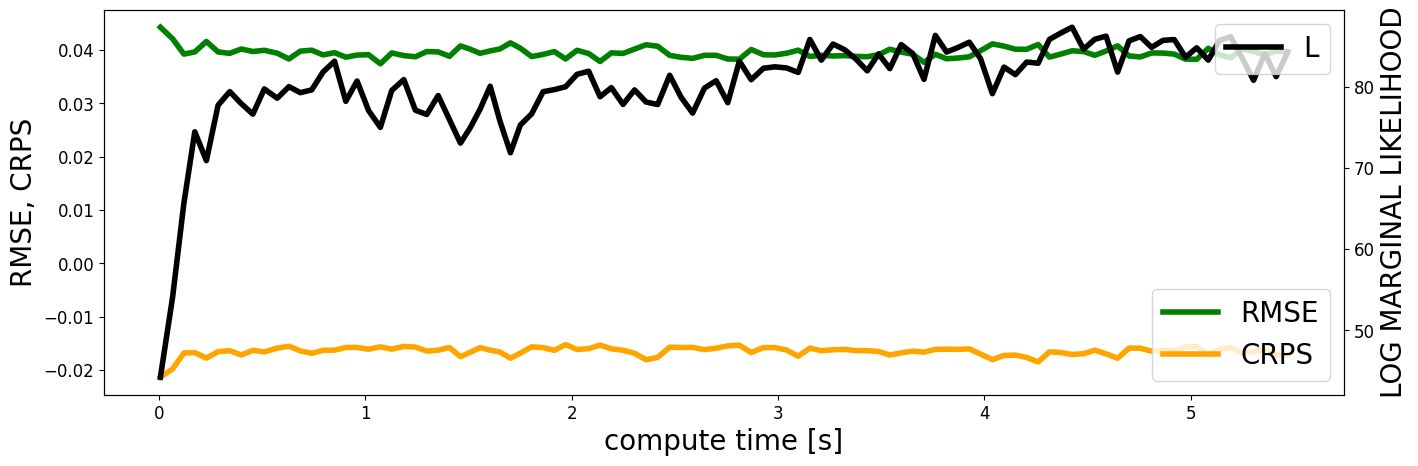
[b]0.8

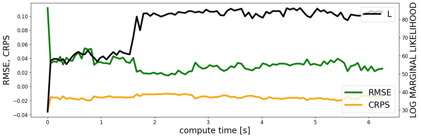
Figure 6: Performance overview for dataset 1. From the top-left: stationary reference kernel, parametric non-stationary kernel, deep kernel, and deep GP. In this test, the parametric non-stationary kernel and the deep kernel reached similar approximation performances, while the former used significantly fewer hyperparameters, which is why it can be trained significantly faster. The deep GP (see Appendix LABEL:app:deepGP for the algorithm), over-smoothed the model and took a long time to train. We note that the deep-GP result highly depended on the specified nugget — too small, and the algorithms produced NaNs, too large, and the presented smoothing was observed. The result was the same when we allowed the algorithm to choose its own nugget. Note the asterisk next to the deep-GP compute time, denoting that this is a separate software written in a different language (R), and compute times can therefore not be directly compared.

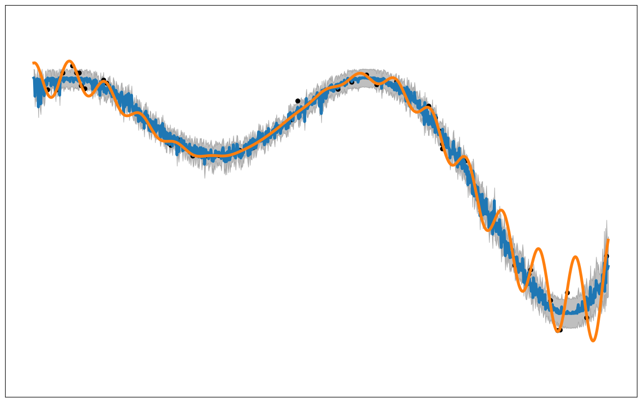
Figure 7: Approximation result for the one-dimensional synthetic dataset using the gpflux DGP. Despite following the online documentation closely, the model appears to show artifacts. This is the reason why we did not use the gpflux DGP for our higher-dimensional test cases. For reproducibility purposes, we publish our exact run script in the Appendix (see LABEL:sec:appA).

4.2.2 The Climate Model

Our three-dimensional climate dataset was introduced in Section 4.1. The stationary reference kernel ($k_{stat}$) is a Matérn kernel with $\nu=3/2$ (Equation 20). In all cases, stationary and non-stationary, we added to the kernel matrix the noise covariance matrix $\mathbf{V}=\sigma^{2}_{n}\mathbf{I}$, where $\sigma^{2}_{n}$ is the nugget variance, treated as an additional hyperparameter. The parametric non-stationary kernel is similar to Equation eq:kpara1d; however, we place radial basis functions eq:rbf at $\{0,0.5,1\}^{3}$ and added a nugget variance, leading to a total of 58 hyperparameters. The deep kernel $k_{nn}(\boldsymbol{\phi}(\mathbf{x}_{i}),\boldsymbol{\phi}(\mathbf{x}_{j})),\leavevmode\nobreak\ \boldsymbol{\phi}:\mathbb{R}^{3}\rightarrow\mathbb{R}^{3}$ has two hidden layers of width 10, but is otherwise identical to eq:knn1d, yielding 186 hyperparameters. The results, two-dimensional slices through the three-dimensional input space, are presented in Figure 8. For completeness, we included the deep GP result in Figure 10, which, however, in our run was not competitive. Once again, the stationary kernel ($k_{stat}$) delivers fast and robust results; however, lacks accuracy compared to the parametric non-stationary kernel ($k_{para}$) and the deep kernel ($k_{nn}$). The performance of the two non-stationary kernels is on par with a slight advantage in CRPS for the deep kernel and a significant advantage in compute time for the parametric non-stationary kernel. The MCMC (Figure 9) sample runs revealed stable convergence, however, at significantly different time scales.

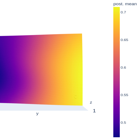
[b]0.45 [b]0.45

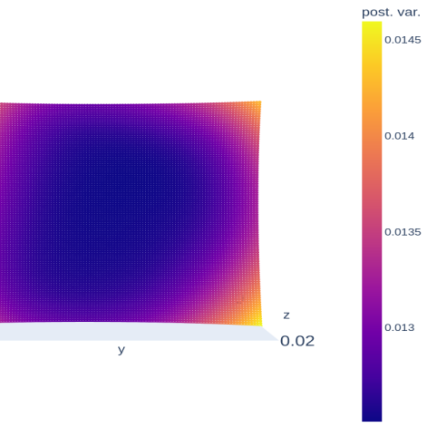
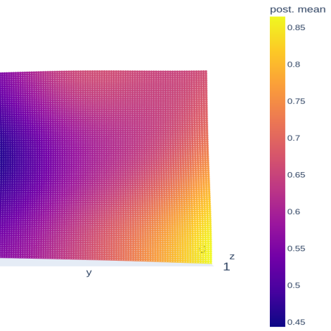
[b]0.45 [b]0.45

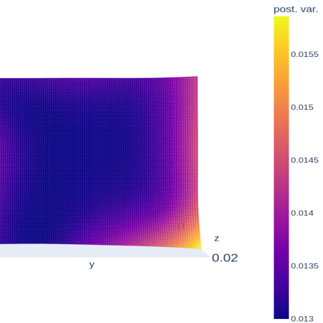
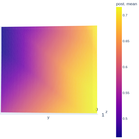
[b]0.45 [b]0.45

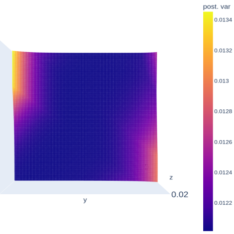
Figure 8: Performance overview for the climate model. From the top: $k_{stat}$, $k_{para}$, and $k_{nn}$. The posterior mean is displayed in the left column. The posterior variance is on the right. The model function is defined over $[0,1]^{2}\times\{0.5\}$. This model is obtained after the convergence of a global evolutionary optimizer. Notable is the fast computing time of the stationary kernel due to the fact that only three hyperparameters have to be found: a signal variance, one isotropic length scale, and the nugget (i.i.d. noise). This parametric non-stationary kernel led to a total number of 58 hyperparameters, which increases the computing time significantly compared to the stationary kernel. The accuracy, in this case, is slightly higher. It is debatable and highly application-driven whether the parametric non-stationary kernel should be used for this dataset. If time is not an issue, the increased accuracy can pay off in downstream operations. The deep kernel contains 186 hyperparameters which are identified robustly. The accuracy of the prediction and the UQ is similar to the parametric non-stationary kernel, with a slight advantage in the CRPS but approximately twice the compute time. As with all our test runs, this run was repeated several times with the same result.

[b]0.8

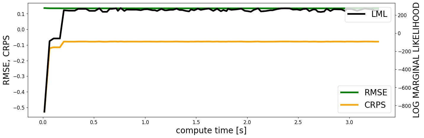
[b]0.8

[b]0.8

Figure 9: MCMC sampling convergence for the climate model and all kernels. From the top: $k_{stat}$, $k_{para}$, and $k_{nn}$. The MCMC is converging robustly but at vastly different time scales; the deep kernel is by far the slowest to converge.

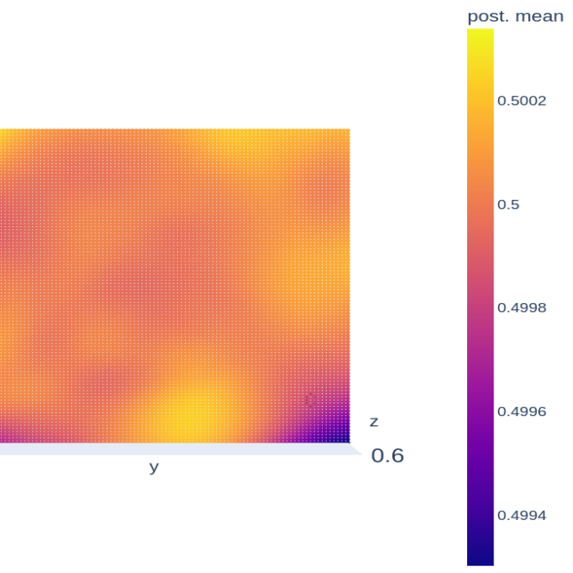
[b]0.45 [b]0.45

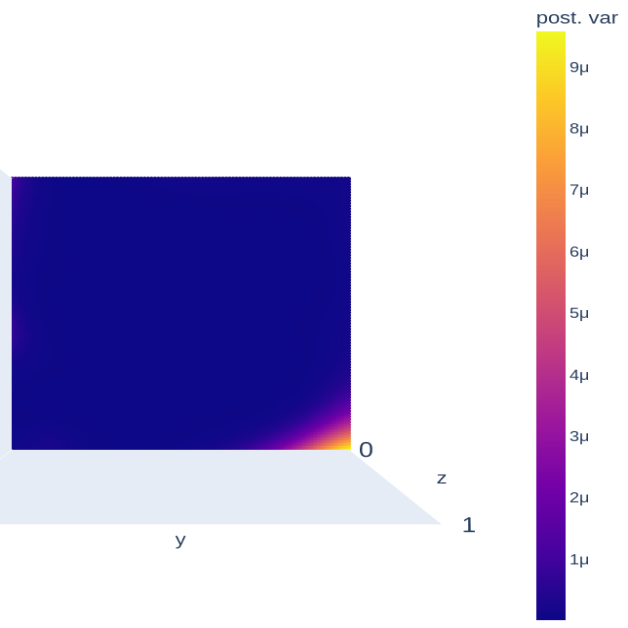
Figure 10: Performance overview for the climate model, computed with the BDGP. The model function — posterior mean (left) and variance (right) — is defined over $[0,1]^{2}\times\{0.5\}$. This result is only presented for completeness. Clearly, our BDGP setup is not competitive compared to the tested kernels. It is presented in Appendix LABEL:sec:appB.

4.2.3 The X-Ray Scattering Model

Our three-dimensional X-ray scattering dataset was introduced in Section 4.1. The kernel setup is identical to our climate example (see Section 4.2.2). The results are presented in Figure 11. This experiment shows improving performance as kernel complexity increases, however, the improvements are moderate. As before, if accuracy is the priority, non-stationary kernels should be considered. Again, the deep kernel ($k_{nn}$) performed very competitively — with a significant advantage in terms of RMSE and CRPS — but did not reach the same log marginal likelihood as the competitors, which can be traced back to solving a high-dimensional optimization due to a large number of hyperparameters. This opens the door to an even better performance if more effort and time is spent in training the model. What stands out in Figure 11 is the smaller and more detailed predicted uncertainties for the deep kernel which would affect decision-making in an online data acquisition context. Also, the posterior mean has more intricate details compared to the stationary and the parametric non-stationary kernel. Figure 12 reveals stable convergence of the MCMC sampling for all kernels at similar time scales supporting the deep kernel as the superior choice on for this model. We again included the BDGP, which however was not competitive (Figure 13).

[b]0.45 [b]0.45

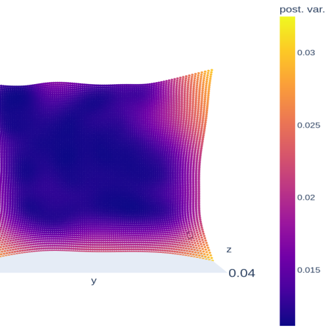
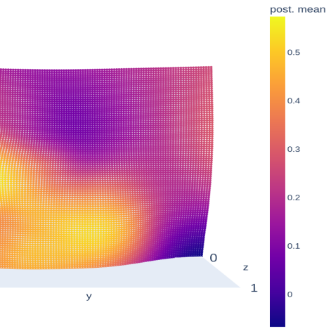
[b]0.45 [b]0.45

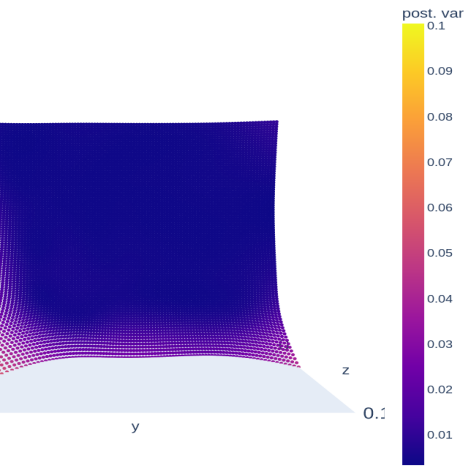
[b]0.45 [b]0.45

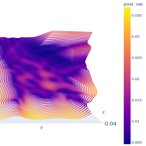
Figure 11: Performance overview for the X-ray model. From the top: $k_{stat}$, $k_{para}$, and $k_{nn}$. The posterior mean is displayed in the left column. The posterior variance is on the right. The model function is defined over $[0,1]^{2}\times\{0.24\}$. This model is obtained after the convergence of a global evolutionary optimizer. Once again, the stationary kernel stands out due to fast computing speeds. The compute time increases significantly for the parametric non-stationary kernel, due to the 58 hyperparameters that have to be found. Since the CRPS is our most relevant performance metric, the approximation and the UQ are better than for the stationary kernel. The deep kernel, for this dataset, performs best with respect to the RMSE and CRPS while achieving lower log marginal likelihood. The training time increases again because 186 hyperparameters have to be found.

[b]0.8

[b]0.8

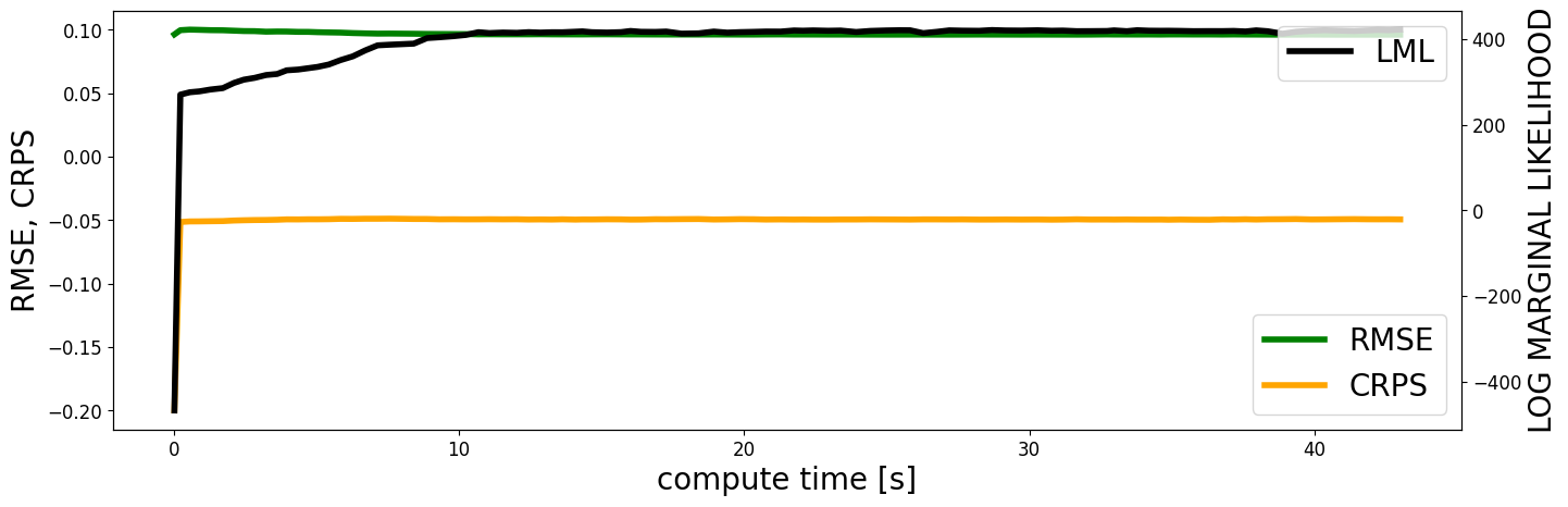
[b]0.8

Figure 12: MCMC sampling convergence for the X-ray model and all kernels. From the top: $k_{stat}$, $k_{para}$, and $k_{nn}$. The MCMC is converging robustly and, in this case, at similar time scales, making the case for the deep kernel that reached the best CRPS.

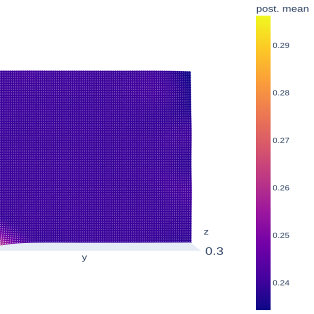
[b]0.45 [b]0.45

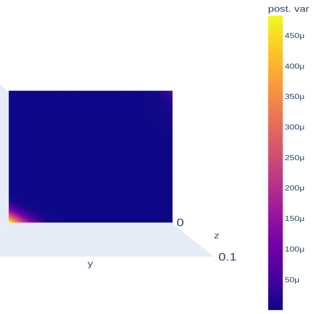
Figure 13: Performance overview for the X-ray scattering model, computed with the BDGP. The model function — posterior mean (left) and variance (right) — is defined over $[0,1]^{2}\times\{0.24\}$. This result is, again, included for completeness; it is not competitive compared to the tested kernels. Our script is presented in Appendix LABEL:sec:appB.

5 Discussion

5.1 Interpretations Test-by-Test

The one-dimensional synthetic function eq:synthfunc exhibits a complex behavior that is captured by our stationarity analysis through the clustering of the length scale versus signal variance and the characteristics observed in the violin plots. The clustering patterns reveal a multifaceted behavior, with different regions of the data exhibiting distinct statistical properties. The linear correlation within one cluster (lower-left, scatter plot, Figure 3) and the dispersion in the other cluster captures the interplay between the sinusoidal and quadratic components of the function. The linear cluster indicates a linear correlation between these two hyperparameters within a specific region of input data. This pattern may correspond to the sinusoidal components of the function, where local oscillations exhibit a consistent relationship between the length scale and signal variance. The additional dispersed points in the scatter plot likely correspond to the regions influenced by the quadratic term in the function, where the statistical properties vary, leading to a broader distribution of the hyperparameters. The bimodal distributions observed in the violin plots for both the length scale and signal variance further corroborate the non-stationarity. These distributions reflect the complexity of the signal, with different modes corresponding to different patterns within the data. The primary modes near zero may correspond to the high-frequency components of the sinusoidal terms, while the secondary mode captures the broader trend introduced by the quadratic term. The signal variance violin plot’s very weak bimodal pattern with a larger variance spread compared to the length scale violin plot reflects the varying magnitude and complexity of the signal. The larger spread in the signal variance captures the diverse behaviors within the synthetic function, including both oscillatory and quadratic patterns. The results provide insights into the intricate interplay between the sinusoidal and quadratic components of the function. The analysis underscores the algorithm’s robustness and sensitivity in measuring non-stationarity across complex data structures, demonstrating its potential as a valuable tool for understanding diverse and multifaceted latent functions. Due to the strong non-stationarity in the data, non-stationary kernels performed extremely well in this case. Due to the low dimensionality, the number of hyperparameters is low in all cases, leading to robust training. It is in our opinion safe to conclude, that in one-dimensional cases, with moderate dataset sizes, and suspected non-stationarity in the data, non-stationary kernels are to be preferred. Both our parametric and deep non-stationary kernels performed well with a slight edge in accuracy for the parametric kernel (see Figure 6). Our two tested deep GP setups (Figures 6 and 7) were not competitive given our reasonable-constraint effort, which in this case, was in the order of days.

Moving on to the climate data example, Figure 4 shows a concentrated cluster near $(0,0)$ and some dispersed points in the length-scale-signal-variance scatter plot which may indicate a strong stationarity in large parts of the input space. This concentration suggests that the statistical properties are consistent across this region, possibly reflecting a dominant pattern or behavior in the data. The presence of fewer dispersed points, forming another much less concentrated cluster, reveals some underlying non-stationarity. In the violin plot, we see a near-unimodal distribution in the signal variance with some weak non-stationarity in the length scale. The computational experiments (see Figures 11) reveal a trade-off between accuracy and compute time. One has to put much more effort — number of hyperparameters and time — into the computation for a relatively small gain in accuracy. Both the parametric non-stationary kernel and the deep kernel achieve higher accuracy than the stationary kernel but are costly. In time-sensitive situations, the stationary kernel is likely to be preferred in this situation; for best accuracy, the parametric non-stationary kernel or the deep kernel is the superior choice. Looking at the CRPS, the deep kernel has a slight edge in accurately estimating uncertainties over the parametric kernel; however, the parametric non-stationary kernel reaches the highest log marginal likelihood. For this dataset, we tested the BDGP without much success under our reasonable-effort constraint (see Figure 10).

Finally, for the X-ray scattering data, Figure 5 shows the presence of a very concentrated cluster near $(0,0)$ in the length-scale-signal-variance scatter plot. This concentration continues to indicate strong stationarity, reflecting consistent statistical properties in much of the domain. However, the inability of the scattered points to form even a weak second cluster represents a significant departure from the climate dataset. The unimodal distributions in the violin plots, with the mode near zero, support the presence of a strong stationary pattern. This leads to similar performances across our test kernels (see Figure 11), with the stationary kernel showing a high RMSE but the worst CRPS, and the deep kernel showing a slight edge in CRPS over its competitors — since stationary kernels only allow us to estimate uncertainties based on global properties of the data and local geometry it is expected that non-stationarity kernels estimate uncertainties more accurately which manifests itself in a higher CRPS. The parametric non-stationary kernel leads the field in log marginal likelihood. Surprisingly, among the three tested kernels, the deep kernel leads to by far the lowest log marginal likelihood, which, again, suggested a better optimizer might lead to a much-improved performance. Once again, our setup of the BDGP was not competitive (see Figure 13).

5.2 Key Takeaways from the Computational Experiments

While we included as much information in the computational experiments and the Appendix as possible to give the reader a chance to make up their own minds, here we summarize some key takeaways.

1. Stationary kernels proved to be surprisingly competitive in terms of the RMSE and are unbeatable when evaluating accuracy per time. It seems worth it in most cases to run a stationary GP first for comparison.

2. Uncertainty is estimated more accurately by non-stationary kernels; if UQ-driven decision-making is the goal, non-stationary kernels are to be preferred. This is not a surprise since, given a constant (possibly anisotropic) length scale and a signal variance, the posterior variance only depends on data-point geometry.

3. The parametric non-stationary kernel encodes a flexible non-stationarity while maintaining interpretability. The involved parametric functions over the input space can be visualized and interpreted.

4. Deep kernels are some of the most flexible kernels but interpretation is lost in all but the simplest cases, which can easily lead to model misspecifications (wrong model class and hyperparameters). Our models took a fair amount of experimenting before an acceptable performance was achieved. In online applications, in which testing beforehand is not possible, deep kernels should be used with caution.

5. Non-stationarity in the covariance structure appears in signal variance and length scale; ideally a kernel addresses both (see Equation 24).

6. While not included in the tests, experimenting with prior mean functions has shown that non-stationarity properties highly depend on the prior mean function of the GP. This is especially true for the non-stationary signal variance.

7. Extrapolation and non-stationary kernels are difficult to combine. While the parametric non-stationary kernel can be set up for extrapolation, traditional neural networks are poorly equipped for that task.

8. We should think of the number of hyperparameters conservatively; too many bear the risk of model misspecification (through local minima) and overfitting.

9. The parametric non-stationary kernel achieved overall better RMSE; the deep kernel led to better uncertainty quantification as indicated by the CRPS.

5.3 A Parametric Deep Kernel

Given the observation that non-stationarity in the covariance structure of a dataset originates from a non-constant signal variance and length scales, one might argue that both should be addressed in the kernel design. Our parametric non-stationary kernel attempts to account for all non-stationary purely through the signal variance; it leaves the length scale constant — however, implementations exist that allow non-constant and anisotropic length scales [Paciorek and Schervish(2006), Risser and Calder(2015)], generally in the same flavor as the parametric non-stationary signal variance. The deep kernel, on the other hand, only acts on the length scale by warping the input space. It seems logical to ask what happens if we combine the two concepts. The kernel

$$k(\mathbf{x}_{i},\mathbf{x}_{j})=\sum_{d=1}^{2}g_{d}(\mathbf{x}_{i})g_{d}(\mathbf{x}_{j})k(\boldsymbol{\phi}(\mathbf{x}_{i}),\boldsymbol{\phi}(\mathbf{x}_{j}))$$ (24)

achieves just that; it is a combination of our parametric non-stationary kernel and the deep kernel. Modeling our synthetic dataset, see Figure 14, we see good performance with moderate improvements compared to our earlier tests (Figure 6). The kernel might constitute somewhat of an overkill for such a simple problem but might lead to more significant gains in real applications. We encourage the reader to give this kernel a try in their next application.

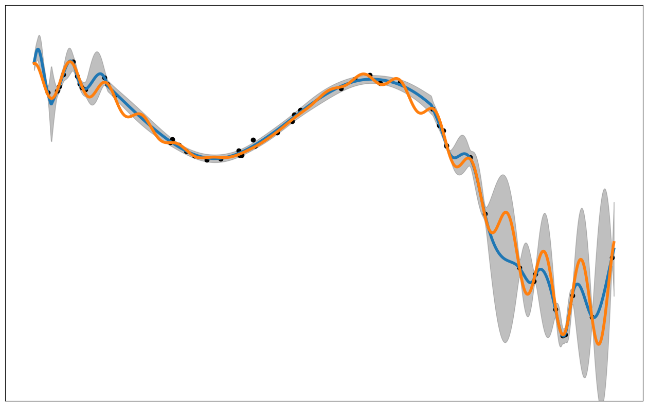
Figure 14: Approximation result for the one-dimensional synthetic dataset using the parametric deep non-stationary kernel eq:newkernel. The kernel combines non-stationarity in the signal variance and the length scale by leveraging both the parametric non-stationarity kernel design and a deep kernel. The approximation is on par with our previously tested methods but the reached likelihood is higher. This kernel might perform very well when strong non-stationarity is present in length scale and signal variance

5.4 Connection between Multi-Task Learning and Non-Stationary Kernels

Multi-task learning offers a powerful paradigm to leverage shared information across multiple related tasks, thereby enhancing the predictive performance of each individual task [Luo and Strait(2022), Sid-Lakhdar et al.((Alphabetic) 2020)Sid-Lakhdar, Cho, Demmel, Luo, Li, Liu, and Marques, Zhu et al.(2022)Zhu, Liu, Ghysels, Bindel, and Li]. This is particularly beneficial when data for some tasks are sparse, as information from data-rich tasks can be used to inform predictions for data-scarce tasks. Flexible non-stationary kernels offer an interesting benefit for multi-task learning: instead of employing specialized techniques, such as coregionalization, one can reformulate the problem to a single task problem and let a flexible non-stationary kernel learn intricate correlations between input ($\mathcal{X}_{i}$) and output ($\mathcal{X}_{o}$) space locations. By transforming the multi-task learning problem over $\mathcal{X}_{i}$ to a single-task learning problem over $\mathcal{X}_{i}\times\mathcal{X}_{o}$, no further changes to the core algorithm are required. This has been known for a long time and is referred to as problem-transformation methods [Borchani et al.(2015)Borchani, Varando, Bielza, and Larranaga]. These methods were originally dismissed as not being able to capture intricate correlations between the tasks; however, this is only true if stationary, separable kernels are used. A flexible non-stationary kernel is able to flexibly encode covariances across the input and the output domain, independent of the indexing of the tasks. This makes it possible to transfer all complexities of multi-task learning to the kernel design and use the rest of the GP framework as-is, inheriting the superior robustness and interpretability properties of single-task GPs.

6 Summary and Conclusion

In this paper, we put on the hat of a machine learning practitioner trying to find the best kernel or methodology within the scope of a Gaussian process (GP) to address non-stationarity in various datasets. We introduced three different datasets — one synthetic, one climate dataset, and one originating from an X-ray scatting experiment at the CMS beamline at NSLSII, Brookhaven National Laboratory. We introduced a non-stationarity measure and studied each dataset to be able to judge their non-stationarity properties quantitatively. We then presented four different methodologies to address the non-stationarity: Ignoring it by using a stationary kernel, a parametric non-stationary kernel, that uses a flexible non-constant signal variance, a deep kernel that uses a neural network to warp the input space, and a deep GP. We set all methodologies up under reasonable effort constraints to allow for a fair comparison; just like a a practitioner might encounter. In our case, that meant minutes of setup time for the stationary kernels and hours to days for the non-stationary kernels and the deep GPs. After the methodologies were set up, we ran our computational tests and presented the results unredacted and uncensored. This way, we hope, the reader gets the best value out of the comparisons. This is also to ensure that the reader has the chance to come up with conclusions different from ours. To further the readers’ ability to double-check and learn, we are publishing all our codes online.

Our tests have shown that even weak non-stationarity in a dataset motivates the use of non-stationary kernels if training time is not an issue of concern. If training time is very limited, stationary kernels are still the preferred choice. We have discovered that non-stationarity in the covariance comes in two flavors, in the signal variance and the length scale and, ideally, both should be addressed through novel kernel designs; we drew attention to one such kernel design. However, non-stationary kernels come with a great risk of model misspecification. If a new model should be relied on out-of-the-box, a stationary kernel might be the preferred choice.

We hope that this paper motivates more practitioners to deploy and experiment with non-stationary kernels but to also be aware of some of the risks.

Acknowledgements

The work was supported by the Laboratory Directed Research and Development Program of Lawrence Berkeley National Laboratory under U.S. Department of Energy Contract No. DE-AC02-05CH11231. This work was further supported by the Regional and Global Model Analysis Program of the Office of Biological and Environmental Research in the Department of Energy Office of Science under contract number DE-AC02-05CH11231. This document was prepared as an account of work sponsored by the United States Government. While this document is believed to contain the correct information, neither the United States Government nor any agency thereof, nor the Regents of the University of California, nor any of their employees, makes any warranty, express or implied, or assumes any legal responsibility for the accuracy, completeness, or usefulness of any information, apparatus, product, or process disclosed, or represents that its use would not infringe privately owned rights. Reference herein to any specific commercial product, process, or service by its trade name, trademark, manufacturer, or otherwise, does not necessarily constitute or imply its endorsement, recommendation, or favoring by the United States Government or any agency thereof, or the Regents of the University of California. The views and opinions of the authors expressed herein do not necessarily state or reflect those of the United States Government or any agency thereof or the Regents of the University of California.

We want to thank Kevin G. Yager from Brookhaven National Laboratory for providing the X-ray scattering dataset. This data collection used resources of the Center for Functional Nanomaterials (CFN), and the National Synchrotron Light Source II (NSLS-II), which are U.S. Department of Energy Office of Science User Facilities, at Brookhaven National Laboratory, funded under Contract No. DE-SC0012704.

Conflict of Interest

The authors declare no conflict of interest.

Data Availability

All data and the Jupyter notebook that runs all experiments can be found on gpcam.lbl.gov/examples/non_stat_kernels (available upon publication).

Code Availibility

All experiments (except deep GPs) were run using the open-source Python package fvGP (github.com/lbl-camera/fvGP) which is available stand-alone and within gpCAM(gpcam.lbl.gov). The run scripts are available at gpcam.lbl.gov/examples/non_stat_kernels (available upon publication).

Author Contributions

M.M.N. originally decided to write this paper, led the project, developed the test scripts and software with help from H.L. and M.R., and ran the computational experiments. H.L. suggested the non-stationarity measure and improved its practicality with help from M.M.N. and M.R. H.L. also did the majority of the work regarding deep GPs, both regarding the algorithms and the manuscript. M.R. oversaw all developments, especially regarding parametric non-stationary kernels, and further assisted with writing and editing the manuscript. All authors iteratively refined the core ideas, algorithms, and methods. All decisions regarding the work were made in agreement with all authors. All authors iteratively revised the manuscript.

APPENDIX

A Theoretical Motivation for Our Non-Stationarity Measure

The simple technique used in this paper is to measure non-stationarity in the covariance structure of a dataset based on the idea of model misspecification. If we assume that the true generating model (i.e., data-generating mechanism that generates the training data) and the fitted GP model both belong to the same model class $\mathcal{M}$ parameterized by the likelihood family $p(\mathbf{y},\mathbf{x}\mid(\sigma_{s},l))$, $(\sigma_{s},l)$ is the stationary-kernel parameterization (the hyperparameters) of a stationary and isotropic GP, then minimizing the KL divergence is equivalent to maximizing the likelihood. Assuming the stationary data-generating model $p(\mathbf{y},\mathbf{x}\mid(\sigma_{s},l)_{2})$ and a stationary GP model likelihood $p(\mathbf{y},\mathbf{x}\mid(\sigma_{s},l)_{1})$, the following argument shows this equivalence.

(σ_s,l)^* & =arg min_(σ_s,l)D_KL(p(y,x—(σ_s,l)_1)——p(y,x—(σ_s,l)_2))
=arg min_(σ_s,l)E_p(y,x—(σ_s,l)_1)[logp(y,x—(σ_s,l)_1)-logp(y,x—(σ_s,l)_2)]
=arg max_(σ_s,l)E_p(y,x—(σ_s,l)_1)[logp(y,x—(σ_s,l)_2)] Now, when the data-generating model and stationary GP models don’t belong to the same model class $\mathcal{M}$, the KL divergence can be decomposed as:

D_KL(p(y, x—(σ_s,l)_1)——p(y, x—(σ_s,l)_2))=(D_KL(p(y, x—(σ_s,l)_1)——M)-D_KL(p(y, x—(σ_s,l)_2)——M))
+D_KL(p(y, x—(σ_s,l)

References

- [Adler(1981)] Robert J. Adler. The Geometry of Random Fields. John Wiley & Sons, 1981.
- [Allenby and Rossi(2006)] Greg M Allenby and Peter E Rossi. Hierarchical bayes models. The handbook of marketing research: Uses, misuses, and future advances, pages 418–440, 2006.
- [Anderes and Stein(2008)] Ethan B. Anderes and Michael L. Stein. Estimating deformations of isotropic Gaussian random fields on the plane. The Annals of Statistics, 36(2):719–741, 04 2008.
- [Barry and Ver Hoef(1996)] Ronald Paul Barry and Jay M Ver Hoef. Blackbox kriging: Spatial prediction without specifying variogram models. Journal of Agricultural, Biological, and Environmental Statistics, 1(3):297–322, 1996.
- [Blomqvist et al.(2020)Blomqvist, Kaski, and Heinonen] Kenneth Blomqvist, Samuel Kaski, and Markus Heinonen. Deep convolutional gaussian processes. In Machine Learning and Knowledge Discovery in Databases: European Conference, ECML PKDD 2019, Würzburg, Germany, September 16–20, 2019, Proceedings, Part II, pages 582–597. Springer, 2020.
- [Bochner et al.(1959)] Salomon Bochner et al. Lectures on Fourier integrals, volume 42. Princeton University Press, 1959.
- [Borchani et al.(2015)Borchani, Varando, Bielza, and Larranaga] Hanen Borchani, Gherardo Varando, Concha Bielza, and Pedro Larranaga. A survey on multi-output regression. Wiley Interdisciplinary Reviews: Data Mining and Knowledge Discovery, 5(5):216–233, 2015.
- [Bornn et al.(2012)Bornn, Shaddick, and Zidek] Luke Bornn, Gavin Shaddick, and James V Zidek. Modeling nonstationary processes through dimension expansion. Journal of the American Statistical Association, 107(497):281–289, 2012.
- [Cutajar et al.(2017)Cutajar, Bonilla, Michiardi, and Filippone] Kurt Cutajar, Edwin V Bonilla, Pietro Michiardi, and Maurizio Filippone. Random feature expansions for deep gaussian processes. In International Conference on Machine Learning, pages 884–893. PMLR, 2017.
- [Dai et al.(2015)Dai, Damianou, González, and Lawrence] Zhenwen Dai, Andreas Damianou, Javier González, and Neil Lawrence. Variational auto-encoded deep gaussian processes. arXiv preprint arXiv:1511.06455, 2015.
- [Damian et al.(2001)Damian, Sampson, and Guttorp] Doris Damian, Paul D Sampson, and Peter Guttorp. Bayesian estimation of semi-parametric non-stationary spatial covariance structures. Environmetrics: The official journal of the International Environmetrics Society, 12(2):161–178, 2001.
- [Damianou and Lawrence(2013)] Andreas Damianou and Neil D Lawrence. Deep gaussian processes. In Artificial intelligence and statistics, pages 207–215. PMLR, 2013.
- [Daniels and Kass(1999)] Michael J Daniels and Robert E Kass. Nonconjugate bayesian estimation of covariance matrices and its use in hierarchical models. Journal of the American Statistical Association, 94(448):1254–1263, 1999.
- [Dunlop et al.(2018)Dunlop, Girolami, Stuart, and Teckentrup] Matthew M Dunlop, Mark A Girolami, Andrew M Stuart, and Aretha L Teckentrup. How deep are deep gaussian processes? Journal of Machine Learning Research, 19(54):1–46, 2018.
- [Dutordoir et al.(2021)Dutordoir, Salimbeni, Hambro, McLeod, Leibfried, Artemev, van der Wilk, Hensman, Deisenroth, and John] Vincent Dutordoir, Hugh Salimbeni, Eric Hambro, John McLeod, Felix Leibfried, Artem Artemev, Mark van der Wilk, James Hensman, Marc P Deisenroth, and ST John. Gpflux: A library for deep gaussian processes. arXiv preprint arXiv:2104.05674, 2021.
- [Fotheringham et al.(2003)Fotheringham, Brunsdon, and Charlton] A Stewart Fotheringham, Chris Brunsdon, and Martin Charlton. Geographically weighted regression: the analysis of spatially varying relationships. John Wiley & Sons, 2003.
- [Gardner et al.(2018)Gardner, Pleiss, Bindel, Weinberger, and Wilson] Jacob R Gardner, Geoff Pleiss, David Bindel, Kilian Q Weinberger, and Andrew Gordon Wilson. Gpytorch: Blackbox matrix-matrix gaussian process inference with gpu acceleration. In Advances in Neural Information Processing Systems, 2018.
- [Geoga et al.(2020)Geoga, Anitescu, and Stein] Christopher J Geoga, Mihai Anitescu, and Michael L Stein. Scalable gaussian process computations using hierarchical matrices. Journal of Computational and Graphical Statistics, 29(2):227–237, 2020.
- [Gramacy and Apley(2015)] Robert B Gramacy and Daniel W Apley. Local gaussian process approximation for large computer experiments. Journal of Computational and Graphical Statistics, 24(2):561–578, 2015.
- [Gramacy and Lee(2008)] Robert B Gramacy and Herbert K H Lee. Bayesian treed gaussian process models with an application to computer modeling. Journal of the American Statistical Association, 103(483):1119–1130, 2008.
- [Grünwald and Van Ommen(2017)] Peter Grünwald and Thijs Van Ommen. Inconsistency of bayesian inference for misspecified linear models, and a proposal for repairing it. 2017.
- [Havasi et al.(2018)Havasi, Hernández-Lobato, and Murillo-Fuentes] Marton Havasi, José Miguel Hernández-Lobato, and Juan José Murillo-Fuentes. Inference in deep gaussian processes using stochastic gradient hamiltonian monte carlo. In Advances in Neural Information Processing Systems, 2018.
- [Hensman et al.(2015)Hensman, Matthews, and Ghahramani] James Hensman, Alexander Matthews, and Zoubin Ghahramani. Scalable variational gaussian process classification. In Artificial Intelligence and Statistics, pages 351–360. PMLR, 2015.
- [Higdon(2002)] Dave Higdon. Space and space-time modeling using process convolutions. In CliveW. Anderson, Vic Barnett, PhilipC. Chatwin, and AbdelH. El-Shaarawi, editors, Quantitative Methods for Current Environmental Issues, pages 37–56. Springer London, 2002.
- [Higdon et al.(2022)Higdon, Swall, and Kern] Dave Higdon, Jenise Swall, and John Kern. Non-stationary spatial modeling. arXiv preprint arXiv:2212.08043, 2022.
- [Higdon(1998)] David Higdon. A process-convolution approach to modelling temperatures in the North Atlantic Ocean. Environmental and Ecological Statistics, 5(2):173–190, 1998.
- [Holland et al.(1998)Holland, Saltzman, Cox, and Nychka] David M. Holland, Nancy Saltzman, Lawrence H. Cox, and Douglas Nychka. Spatial prediction of dulfur dioxide in the eastern United States. In Jaime Gomez-Hernandez, Amilcar Soares, and Roland Friodevaux, editors, GeoENV II: Geostatistics for Environmental Applications., pages 65–75. Kluwer Academic Publishers, 1998.
- [Ickstadt and Wolpert(1998)] Katja Ickstadt and Robert L. Wolpert. Spatial regression for marked point processes. Bayesian Statistics, 6, 1998.
- [Jimenez and Katzfuss(2023)] Felix Jimenez and Matthias Katzfuss. Vecchia gaussian process ensembles on internal representations of deep neural networks. arXiv preprint arXiv:2305.17063, 2023.
- [Jones et al.(2023)Jones, Townes, Li, and Engelhardt] Andrew Jones, F William Townes, Didong Li, and Barbara E Engelhardt. Alignment of spatial genomics data using deep gaussian processes. Nature Methods, pages 1–9, 2023.
- [Karhunen(1946)] Kari Karhunen. Zur spektraltheorie stochastischer prozesse. Ann. Acad. Sci. Fennicae, AI, 34, 1946.
- [Kleijn and van der Vaart(2006)] Bas JK Kleijn and Aad W van der Vaart. Misspecification in infinite-dimensional bayesian statistics. 2006.
- [Kleijn and Van der Vaart(2012)] Bas JK Kleijn and Aad W Van der Vaart. The bernstein-von-mises theorem under misspecification. 2012.
- [Lin et al.(2023)Lin, Antorán, Padhy, Janz, Hernández-Lobato, and Terenin] Jihao Andreas Lin, Javier Antorán, Shreyas Padhy, David Janz, José Miguel Hernández-Lobato, and Alexander Terenin. Sampling from gaussian process posteriors using stochastic gradient descent. arXiv preprint arXiv:2306.11589, 2023.
- [Litvinenko et al.(2019)Litvinenko, Sun, Genton, and Keyes] Alexander Litvinenko, Ying Sun, Marc G Genton, and David E Keyes. Likelihood approximation with hierarchical matrices for large spatial datasets. Computational Statistics & Data Analysis, 137:115–132, 2019.
- [Loeve(1955)] Michel Loeve. Probability theory : foundations , random sequences. 1955.
- [Luo and Pratola(2022)] Hengrui Luo and Matthew T. Pratola. Sharded Bayesian Additive Regression Trees. Under rev., pages 1–46, 2022.
- [Luo and Strait(2022)] Hengrui Luo and Justin D. Strait. Nonparametric Multi-shape Modeling with Uncertainty Quantification. arXiv:2206.09127, pages 1–52, 2022.
- [Luo et al.(2022)Luo, Nattino, and Pratola] Hengrui Luo, Giovanni Nattino, and Matthew T Pratola. Sparse additive Gaussian process regression. Journal of Machine Learning Research, 23(61):1–34, 2022.
- [Mohamed(2015)] Shakir Mohamed. A statistical view of deep learning. ArXiv e-prints, 2015.
- [Noack and Reyes(2023)] Marcus M Noack and Kristofer G Reyes. Mathematical nuances of Gaussian process-driven autonomous experimentation. MRS Bulletin, pages 1–11, 2023.
- [Noack and Sethian(2022)] Marcus M Noack and James A Sethian. Advanced stationary and nonstationary kernel designs for domain-aware Gaussian processes. Communications in Applied Mathematics and Computational Science, 17(1):131–156, 2022.
- [Noack et al.(2021)Noack, Zwart, Ushizima, Fukuto, Yager, Elbert, Murray, Stein, Doerk, Tsai, et al.] Marcus M Noack, Petrus H Zwart, Daniela M Ushizima, Masafumi Fukuto, Kevin G Yager, Katherine C Elbert, Christopher B Murray, Aaron Stein, Gregory S Doerk, Esther HR Tsai, et al. Gaussian processes for autonomous data acquisition at large-scale synchrotron and neutron facilities. Nature Reviews Physics, 3(10):685–697, 2021.
- [Noack et al.(2023)Noack, Krishnan, Risser, and Reyes] Marcus M Noack, Harinarayan Krishnan, Mark D Risser, and Kristofer G Reyes. Exact Gaussian processes for massive datasets via non-stationary sparsity-discovering kernels. Scientific reports, 13(1):3155, 2023.
- [Nychka et al.(2002)Nychka, Wikle, and Royle] Douglas Nychka, Christopher Wikle, and J Andrew Royle. Multiresolution models for nonstationary spatial covariance functions. Statistical Modelling, 2(4):315–331, 2002.
- [Ober et al.(2021)Ober, Rasmussen, and van der Wilk] Sebastian W Ober, Carl E Rasmussen, and Mark van der Wilk. The promises and pitfalls of deep kernel learning. In Uncertainty in Artificial Intelligence, pages 1206–1216. PMLR, 2021.
- [Paciorek and Schervish(2003)] Christopher Paciorek and Mark Schervish. Nonstationary covariance functions for gaussian process regression. Advances in neural information processing systems, 16, 2003.
- [Paciorek and Schervish(2006)] Christopher J Paciorek and Mark J Schervish. Spatial modelling using a new class of nonstationary covariance functions. Environmetrics: The official journal of the International Environmetrics Society, 17(5):483–506, 2006.
- [Picheny and Ginsbourger(2013)] Victor Picheny and David Ginsbourger. A nonstationary space-time gaussian process model for partially converged simulations. SIAM/ASA Journal on Uncertainty Quantification, 1(1):57–78, 2013.
- [Pilario et al.(2020)Pilario, Shafiee, Cao, Lao, and Yang] Karl Ezra Pilario, Mahmood Shafiee, Yi Cao, Liyun Lao, and Shuang-Hua Yang. A review of kernel methods for feature extraction in nonlinear process monitoring. Processes, 8(1):24, 2020.
- [Ranganath et al.(2014)Ranganath, Tang, Charlin, and Blei] Rajesh Ranganath, Linpeng Tang, Laurent Charlin, and David M Blei. Deep exponential families. arXiv preprint arXiv:1411.2581, 2014.
- [Risser and Calder(2015)] Mark D Risser and Catherine A Calder. Regression-based covariance functions for nonstationary spatial modeling. Environmetrics, 26(4):284–297, 2015.
- [Salakhutdinov and Larochelle(2010)] Ruslan Salakhutdinov and Hugo Larochelle. Efficient learning of deep boltzmann machines. In Proceedings of the thirteenth international conference on artificial intelligence and statistics, pages 693–700. JMLR Workshop and Conference Proceedings, 2010.
- [Salimbeni and Deisenroth(2017)] Hugh Salimbeni and Marc Deisenroth. Doubly stochastic variational inference for deep gaussian processes. Advances in neural information processing systems, 30, 2017.
- [Salimbeni et al.(2019)Salimbeni, Dutordoir, Hensman, and Deisenroth] Hugh Salimbeni, Vincent Dutordoir, James Hensman, and Marc Deisenroth. Deep gaussian processes with importance-weighted variational inference. In International Conference on Machine Learning, pages 5589–5598. PMLR, 2019.
- [Sampson and Guttorp(1992)] Paul D Sampson and Peter Guttorp. Nonparametric estimation of nonstationary spatial covariance structure. Journal of the American Statistical Association, 87(417):108–119, 1992.
- [Sauer et al.(2022)Sauer, Cooper, and Gramacy] Annie Sauer, Andrew Cooper, and Robert B Gramacy. Vecchia-approximated deep gaussian processes for computer experiments. Journal of Computational and Graphical Statistics, pages 1–14, 2022.
- [Sauer et al.(2023)Sauer, Cooper, and Gramacy] Annie Sauer, Andrew Cooper, and Robert B Gramacy. Non-stationary gaussian process surrogates. arXiv preprint arXiv:2305.19242, 2023.
- [Schabenberger and Gotway(2017)] Oliver Schabenberger and Carol A Gotway. Statistical methods for spatial data analysis. CRC press, 2017.
- [Schervish(2012)] Mark J Schervish. Theory of statistics. Springer Science & Business Media, 2012.
- [Schmidt and O’Hagan(2003)] Alexandra M Schmidt and Anthony O’Hagan. Bayesian inference for non-stationary spatial covariance structure via spatial deformations. Journal of the Royal Statistical Society Series B: Statistical Methodology, 65(3):743–758, 2003.
- [Scott et al.(2016)Scott, Blocker, Bonassi, Chipman, George, and McCulloch] Steven L. Scott, Alexander W. Blocker, Fernando V. Bonassi, Hugh A. Chipman, Edward I. George, and Robert E. McCulloch. Bayes and big data: The consensus monte carlo algorithm. International Journal of Management Science and Engineering Management, 11:78–88, 2016.
- [Sid-Lakhdar et al.((Alphabetic) 2020)Sid-Lakhdar, Cho, Demmel, Luo, Li, Liu, and Marques] Wissam M. Sid-Lakhdar, Younghyun Cho, James W. Demmel, Hengrui Luo, Xiaoye S. Li, Yang Liu, and Osni Marques. GPTune User Guide, (Alphabetic) 2020.
- [Snelson and Ghahramani(2005)] Edward Snelson and Zoubin Ghahramani. Sparse gaussian processes using pseudo-inputs. Advances in neural information processing systems, 18, 2005.
- [Snoek et al.(2012)Snoek, Larochelle, and Adams] Jasper Snoek, Hugo Larochelle, and Ryan P Adams. Practical bayesian optimization of machine learning algorithms. Advances in neural information processing systems, 25, 2012.
- [Stein(1999)] Michael L Stein. Interpolation of spatial data: some theory for kriging. Springer Science & Business Media, 1999.
- [Stein(2005)] Michael L Stein. Nonstationary spatial covariance functions. Unpublished technical report, 2005.
- [Teh et al.(2004)Teh, Jordan, Beal, and Blei] Yee Teh, Michael Jordan, Matthew Beal, and David Blei. Sharing clusters among related groups: Hierarchical dirichlet processes. Advances in neural information processing systems, 17, 2004.
- [Thiébaux(1976)] H. Jean Thiébaux. Anisotropic correlation functions for objective analysis. Monthly Weather Review, 104:994–1002, 1976.
- [Thiébaux and Pedder(1987)] H. Jean Thiébaux and M. A. Pedder. Spatial objective analysis: with applications in atmospheric science. Academic Press, 1987.
- [Titsias and Lawrence(2010)] Michalis Titsias and Neil D Lawrence. Bayesian gaussian process latent variable model. In Proceedings of the thirteenth international conference on artificial intelligence and statistics, pages 844–851. JMLR Workshop and Conference Proceedings, 2010.
- [Ver Hoef et al.(2004)Ver Hoef, Cressie, and Barry] Jay M Ver Hoef, Noel Cressie, and Ronald Paul Barry. Flexible spatial models for kriging and cokriging using moving averages and the fast fourier transform (fft). Journal of Computational and Graphical Statistics, 13(2):265–282, 2004.
- [Wikle(2010)] Christopher K. Wikle. Low-rank representations for spatial processes. In A.E. Gelfand, M. Fuentes, P. Guttorp, and P. Diggle, editors, Handbook of Spatial Statistics, Chapman & Hall/CRC Handbooks of Modern Statistical Methods. Taylor & Francis, 2010.
- [Williams and Rasmussen(2006)] Christopher KI Williams and Carl Edward Rasmussen. Gaussian processes for machine learning, volume 2. MIT press Cambridge, MA, 2006.
- [Wilson et al.(2016)Wilson, Hu, Salakhutdinov, and Xing] Andrew Gordon Wilson, Zhiting Hu, Ruslan Salakhutdinov, and Eric P Xing. Deep kernel learning. In Artificial intelligence and statistics, pages 370–378. PMLR, 2016.
- [Wipf and Nagarajan(2007)] David Wipf and Srikantan Nagarajan. A new view of automatic relevance determination. Advances in neural information processing systems, 20, 2007.
- [Zammit-Mangion et al.(2022)Zammit-Mangion, Ng, Vu, and Filippone] Andrew Zammit-Mangion, Tin Lok James Ng, Quan Vu, and Maurizio Filippone. Deep compositional spatial models. Journal of the American Statistical Association, 117(540):1787–1808, 2022.
- [Zhu et al.(2022)Zhu, Liu, Ghysels, Bindel, and Li] Xinran Zhu, Yang Liu, Pieter Ghysels, David Bindel, and Xiaoye S Li. GPTuneBand: Multi-task and multi-fidelity autotuning for large-scale high performance computing applications. In Proceedings of the 2022 SIAM Conference on Parallel Processing for Scientific Computing, pages 1–13. SIAM, 2022.