Cosmology on a Gravitational Wave Background

Abstract

It is a fact that the universe lives on a Gravitational Wave Background (GWB), which it may be in the form of extra energy, which is not contained in Einstein’s field equations. In Matos:2021jef , a new model was developed to explain the current accelerating expansion of the universe where a GWB was incorporated by extending Einstein’s equations to $R_{\mu\nu}-\frac{1}{2}Rg_{\mu\nu}+\frac{2\pi^{2}}{{\lambda}^{2}}g_{\mu\nu}=\kappa^{2}T_{\mu\nu}$, where ${\lambda}$ is the Compton wavelength of the graviton. In the present work we show that this extended form agrees very well with the observations of Cosmic chronometers, Baryon Acoustic Oscillations and Pantheon SN type Ia, reproducing the observational data with a $\Delta\chi^{2}=3.26$ in favor of the present model compared to the $\Lambda$CDM. The values favored by these observations are $\Omega_{\rm m}=0.31\pm 0.02$, $H_{0}=68\pm 0.02$ Km/s/Mpc, $\Omega_{\rm k}=0.001\pm 0.011$; we also find an excellent consistence of this model with the Cosmic Microwave Background and the Matter Power Spectrum. We conclude that this model is an excellent alternative to explain the accelerating expansion of the universe without incorporating the cosmological constant.

I Introduction

In the realm of cosmology, one of the most significant revelations of the past century was the observation that the universe is not only expanding but also experiencing accelerated expansion. This extraordinary finding defied our expectations and sparked research endeavors to comprehend the underlying causes driving this peculiar behavior. It is within this context that the concept of Dark Energy emerged as a compelling explanation for the accelerated expansion. However, the fundamental nature of Dark Energy still remains a perplexing enigma, and unraveling its mysteries continues to be a captivating pursuit. Despite the multitude of proposals and ideas aimed to decipher this phenomenon, we have not yet arrived to a fully convincing solution (see, for instance, Poulin:2023lkg ; Bamba:2022jyz ; Frusciante:2019xia ).

In a previous study Matos:2021jef , a novel model dubbed as the Compton Mass Dark Energy (CMaDE) was introduced, whose main goal is to incorporate the quantum nature of the gravitational field into Einstein’s equations, which could also be considered as the Gravitational Waves Background (GWB), and it could be a viable explanation of the accelerated expansion of the universe. Very recently it has been demonstrated by several observatories that the universe is immersed in a GWB NANOGrav:2023gor ; Reardon:2023gzh ; Xu:2023wog ; Antoniadis:2023lym , in this case the frequencies observed are of the order of nanohertz and their origin is still unknown. However, there is no clear justification for restricting the GWB solely to nanohertz frequencies and therefore we will consider their wavelength may be extended to other scales, specifically those on cosmological scales. In this context, we let the specific origin of the GWB for other works, but it is important to clarify that it is an additional energy not incorporated into the Einstein’s equations a priori, which is intrinsically connected to the space-time metric. Thus, similar to the aforementioned study, the proposal is to incorporate the gravitational wave energy of spacetime into Einstein’s equations. Gravitational waves and the mediator of the gravitational interaction, here for simplicity named as graviton, has zero mass. To study the universe we focus on frequencies on cosmological scales. In Matos:2021jef (see also Escobar-Aguilar:2023ekv ) this energy was introduced into the Einstein equation to obtain

$$R^{\mu\nu}-\frac{1}{2}g^{\mu\nu}R+\frac{2\pi^{2}}{{\lambda}^{2}}g^{\mu\nu}=\kappa^{2}T^{\mu\nu},$$ (1)

where $\kappa^{2}=8\pi G/c^{4}$; $G$ is Newton’s gravitational constant and ${\lambda}$ is the cosmological Compton wavelength of the graviton, which for cosmological scales depends only on the time $t$ coordinate due to the expansion of the universe. For a similar approach, but with a completely different philosophy, see for example Li:2004rb ; Cai:2007us .

In a previous study Matos:2022jzf , it was demonstrated that these equations not only provide an explanation for the accelerated expansion of the universe but may also exhibit an agreement with key cosmological observations such as the Mass Power Spectrum (MPS) and the Cosmic Microwave Background (CMB) radiation. However, it is worth noting that the aforementioned works Matos:2021jef and Matos:2022jzf , were performed by an approximation where the covariant derivative of the energy-momentum tensor ${T^{\mu\nu}}_{;\nu}$ vanished. Although this approximation results in a minimal violation of the general principle of covariance, it is important to address this issue. Therefore, in the present study, we aim to remove the approximation and evaluate the performance of the CMaDE model against the standard $\Lambda$CDM model by confronting it with background data.

II The CMaDE model

Figure 1: In the left panel we show the relationship of the Hubble parameters through $1-H_{\rm{CMaDE}}/H_{\rm{LCDM}}$, from the solutions of the set of equations (II). We notice a similar behaviour, with a few percent level difference at small redshift. Here we set $\mathcal{H}_{0}=1$, $\Omega^{0}_{\rm{0b}}=0.044$, $\Omega^{0}_{\rm{0dm}}=0.27$, $\Omega^{0}_{\rm{0r}}=9.539\times 10^{-5}$ and $\Omega^{0}_{\rm{0k}}=0.08$ for both models. In the left panel we see the evolution of EoS (12) in equation (II). Notice that the effective EoS converges to $-1$ at high redshifts, specially on the recombination epoch.

In order to obtain the conservation equations of the system, in a FLRW universe, we perform the covariant derivative of equation (1). Observe that ${G^{\mu\nu}}_{;\nu}=0$ by construction and ${g^{\mu\nu}}_{;\nu}=0$ because the metric is compatible with respect to the connection. For index $\mu\not=0$ the covariant derivative of equation (1) is an identity, but for $\mu=0$, we obtain

$$\dot{\mathcal{M}}c^{2}=-\kappa^{2}\left(\dot{\rho}+3H(\rho+p)\right),$$ (2)

where

$${\mathcal{M}}=\frac{2\pi^{2}}{\lambda^{2}},$$ (3)

is the extra term in the Einstein’s equations; where $H=\dot{a}/a$ is the Hubble parameter and $\rho$ and $p$ are the total energy density and pressure of the system, respectively. Here, we consider the components of the universe are the matter $\rho_{\rm m}$, which is made up of dark matter $\rho_{\rm dm}$ and baryons $\rho_{\rm b}$, and radiation $\rho_{\rm r}$ made up of neutrinos $\rho_{\nu}$ and photons $\rho_{\gamma}$. Bearing in mind we know the equations of state for baryons and radiation, hence $\dot{\rho}_{\rm b}+3H\rho_{\rm b}=0$ and $\dot{\rho}_{\rm r}+4H\rho_{\rm r}=0$, then we can plug in these results into equation (2). On the other hand, because the lack of information about the nature of the dark matter, as a first approximation we can assume it is made up of dust with $p_{\rm dm}=0$, just like baryons. The main difference with the previous works Matos:2021jef ; Matos:2022jzf is that here we let the dark matter interact with the GWB energy of space-time, avoiding the violation of the general covariance principle. Furthermore, we know that $\rho=\rho_{\rm m}+\rho_{\rm r}=\rho_{\rm dm}+\rho_{\rm b}+\rho_{\rm r}$, and $p=p_{\rm r}+p_{\rm m}=\frac{1}{3}\rho_{\rm r}$. Using these results, the equation (2) becomes

$$k_{c}\dot{\mathcal{M}}c^{2} = -\kappa^{2}\left(\dot{\rho}_{\rm dm}+3H\rho_{\rm dm}\right),$$

$$\dot{\rho}_{\rm b} = -3H\rho_{\rm b},$$

$$\dot{\rho}_{\rm r} = -4H\rho_{\rm r},$$ (4)

where $k_{c}$ is a bias parameter that mediates the contribution of the space-time energy of the GWB to the dark matter.

Next we derive an equation for ${\mathcal{M}}$. We know that the wavelength ${\lambda}$ satisfies the relation ${\lambda}=(c/H_{0})R_{H}$ Matos:2021jef , with

$$R_{H}=H_{0}\int\frac{dt}{a}=H_{0}\int\frac{e^{-N}}{H}dN.$$ (5)

It is convenient to use the e-folding coordinate $N$ defined as $N=\ln(a)$. We denote the derivative with respect to $t$ with an over dot, and a prime means the derivative with respect to $N$. Then, from (3) we have that

$${\mathcal{M}}^{\prime}=-\frac{4\pi^{2}}{{\lambda}^{3}}{\lambda}^{\prime}.$$ (6)

Thus, we use equation (5) to obtain

$${\mathcal{M}}^{\prime}=\pm\frac{\sqrt{2}c}{\pi}{\mathcal{M}}^{3/2}\frac{e^{-N}}{H}.$$ (7)

However, different frequencies of the fluctuations may contribute in a different way to the accelerated expansion, that is, part of these fluctuations can be transformed into black holes, structures of the universe, etc. To mediate this contribution, we can set a bias parameter $Q$ in front of the equation (7). Equations (II) together with the Friedmann equation

$$H^{2}+\frac{k}{a^{2}}-\frac{{\mathcal{M}}c^{2}}{3}=\frac{\kappa^{2}\rho}{3},$$ (8)

where $k=1,-1,0$, is the curvature parameter, are a complete set of equations for the variables $\rho_{\rm b}$, $\rho_{\rm r}$, $\rho_{\rm dm}$ and ${\mathcal{M}}$. It is convenient to rewrite these equations in terms of dimensionless quantities, then we introduce

$$\Omega_{X}^{0}=\frac{\rho_{X}\kappa^{2}}{3H_{0}^{2}}=\Omega^{0}_{0X}a^{-3(1+\omega_{X})},$$ (9)

for each component of the system and $\mathcal{H}=H/H_{0}$, where the second identity is valid only for barotropic fluids with $\omega_{X}=$ constant. Observe that in the definition of $\Omega_{X}^{0}$ we use $H_{0}$ instead of the traditional $H$. Therefore, we obtain a complete system of equations

$$\mathcal{H}^{2} = \Omega^{0}_{\rm b}+\Omega^{0}_{\rm dm}+\Omega^{0}_{\rm r}+\Omega^{0}_{0k}e^{-2N}+\Omega^{0}_{\mathcal{M}},$$

$$\Omega^{0^{\prime}}_{\rm dm} = -3\Omega^{0}_{\rm dm}-k_{c}\Omega^{0^{\prime}}_{\mathcal{M}},$$

$$\Omega^{0^{\prime}}_{\rm b} = -3\Omega^{0}_{\rm b},$$

$$\Omega^{0^{\prime}}_{\rm r} = -4\Omega^{0}_{\rm r},$$

$$\Omega^{0^{\prime}}_{\mathcal{M}} = Q\frac{\sqrt{6}}{\pi}{\Omega^{0}_{\mathcal{M}}}^{3/2}\frac{e^{-N}}{\mathcal{H}},$$ (10)

where the first one is the Friedmann equation. Observe that due to the $\pm$ sign of the square root of $\mathcal{M}$, we have the possibilities that $Q$ can be positive or negative in the evolution of $H$.

Figure 2: Functional posterior probability of the reconstruction with flat curvature. The probability as normalised in each slice of constant $z$, with colour scale in confidence interval values. The 68% ($1\sigma$) and 95% ($2\sigma$) confidence intervals are plotted as black lines. Left: the effective EoS 12 and Right: the Hubble Parameter $H(z)/(1+z)$. The dashed black line corresponds to the standard $\Lambda$CDM values.

Figure 3: Triangular marginal posterior distributions for the inferred parameters; 1D posteriors are displayed over the diagonal and 2D below it; they are colour coded with the inclusion of curvature and the Planck information as shown in the labels.

Figure 4: Top: The CMB and the MPS profiles for the CMaDE model. In this figure we set $H_{0}=72.6$ Km/s/Mpc, $\Omega_{0\rm{b}}=0.044$ and $\Omega_{0\rm{k}}=0$. Bottom: The CMB and the MPS profiles for the CMaDE model. In this figure we set $H_{0}=68$ km/s/Mpc, $\Omega_{0b}=0.048$, $\Omega_{0\rm{DM}}=0.23$ and $\Omega_{0\rm{k}}=0.001$.

III Comparing with Cosmological observations

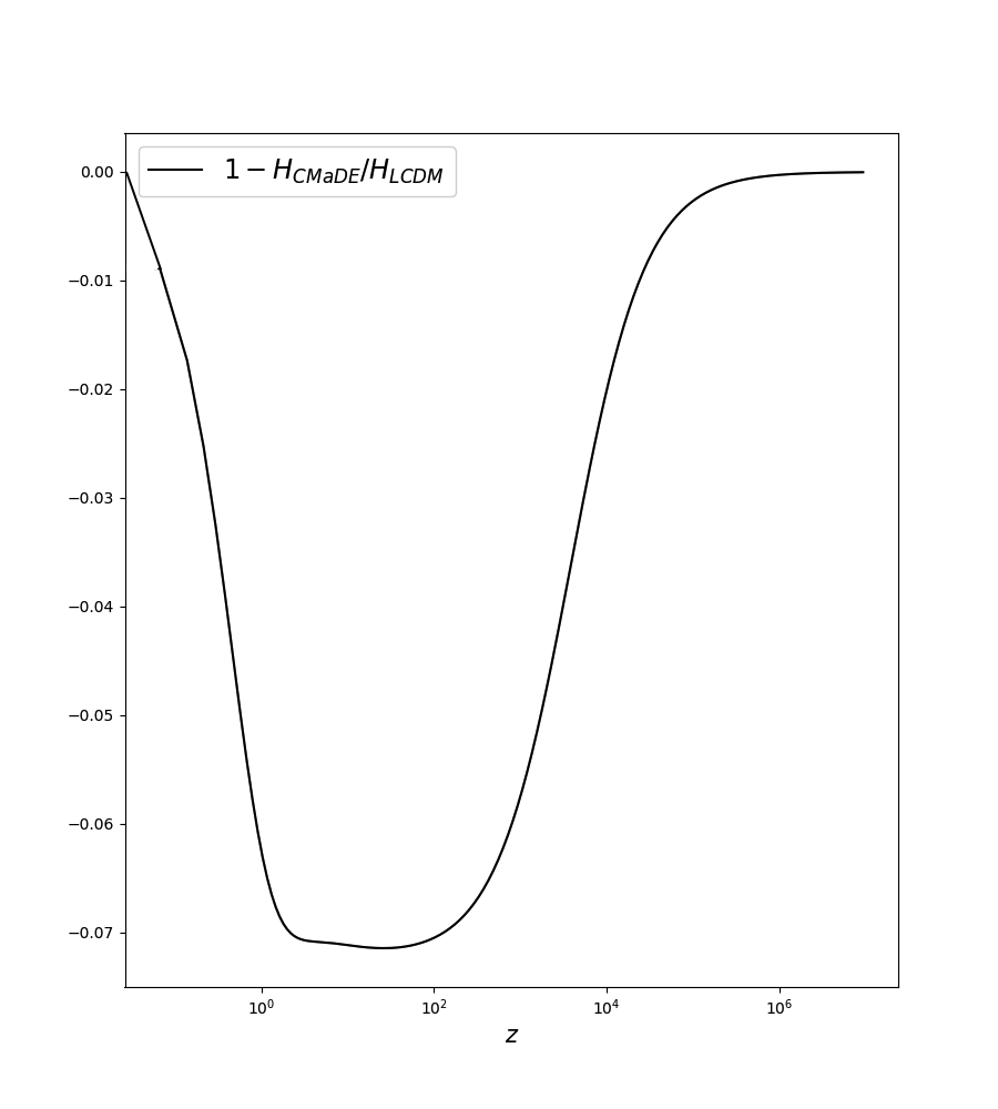
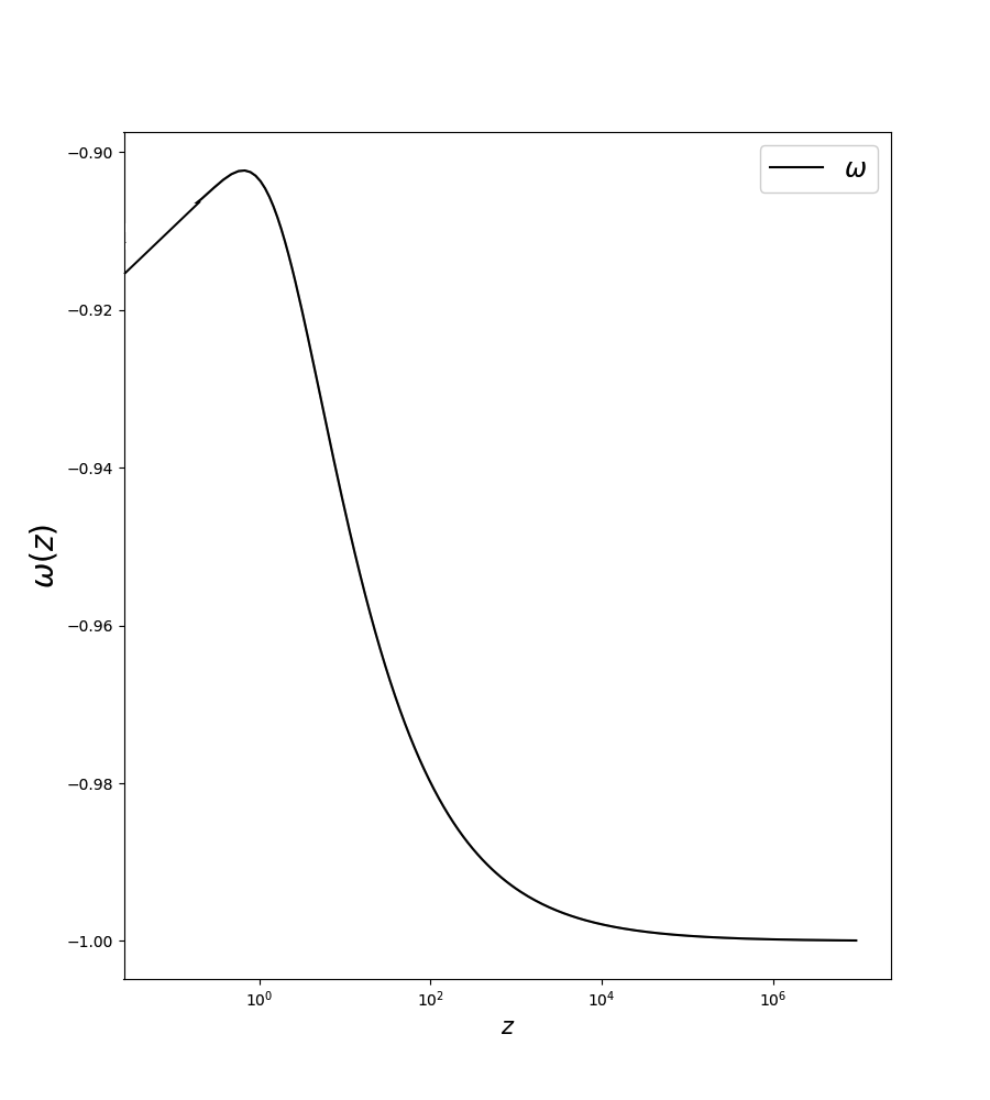
It is straightforward to find numerical solutions of the system (II); as a test we use the initial conditions obtained from the Lambda Cold Dark Matter ($\Lambda$CDM) model, and implemented a python code with an Adams–Badsforth–Moulton algorithm that integrates the system from $N=0$ to $N=-7$. As a proof of the concept, we set as initial conditions $\mathcal{H}_{0}=1$, $\Omega^{0}_{0b}=0.044$, $\Omega^{0}_{0\rm{dm}}=0.27$, $\Omega^{0}_{0\rm{r}}=9.539\times 10^{-5}$ and $\Omega^{0}_{0\rm{k}}=0.08$ for both, the CMaDE and the $\Lambda$CDM models. In figure 1 we show a comparison of the Hubble parameter behaviour for the CMaDE and $\Lambda$CDM models. In the left panel of this figure we establish the current value of the Hubble constant $H_{0}=1$ to compare both evolutions. We plot the rate $1-H_{\rm{CMaDE}}/H_{\rm{LCDM}}$ in order to see the difference between both models and notice its difference does increase at small redshifts, within observable regions, but converges to the $\Lambda$CDM at the present time and as well as at the early universe. We think this could be an indication that the CMaDE model might ameliorate the Hubble constant tension by maintaining consistency with the CMB and modifying mainly the late time observables.

Now we introduce an effective equation of state (EoS) for the CMaDE model. In order to do so, we define a function $w_{\rm eff}$ such that

$$\Omega^{0^{\prime}}_{\mathcal{M}}+3(1+w_{\rm eff})\Omega^{0}_{\mathcal{M}}=0.$$ (11)

We use the last equation of system (II) to obtain the effective equation of state

$$w_{\rm eff}=-Q\sqrt{\frac{2}{3}}\sqrt{\Omega^{0}_{\mathcal{M}}}\frac{e^{-N}}{\pi\mathcal{H}}-1.$$ (12)

We plot the results in the right panel in Fig. 1. Note that the EoS tends to $-1$ in the early universe, then changes its value after recombination. We will see that the CMB values are very much in agreement with this behaviour.

Finally we want to compare the CMaDE model with the main cosmological observations at the background level, and let the perturbative study for future works. In order to do this we performed a statistical analysis of our model parameter space with a publicly available Bayesian inference code named SimpleMC simplemc ; aubourg2015cosmological , which includes the dynesty library speagle2020dynesty , a nested sampling algorithm used to compute the Bayesian evidence. The data sets used in this work consist of:

• Baryon Acoustic Oscillations (BAO) measurements. The BAOs utilized in this study are obtained from SDSS, SDSS-II, BOSS, and eBOSS. The data sets encompass the SDSS Galaxy Consensus, quasars, and Lyman-$\alpha$ forests alam2017clustering ; de2019baryon ; ata2018clustering ; blomqvist2019baryon ; beutler20116df ; eBOSS:2020yzd . The sound horizon is calibrated by using Big Bang Nucleosynthesis aubourg2015cosmological . Henceforth, these measurements will be referred to as BAO.

• The complete catalog of supernovae from the Pantheon Plus SN Ia sample (referred to as SN). This SN data set builds upon the original Pantheon compilation, aiming to enhance the precision and inclusiveness of the supernova sample. Both the covariance matrix and the data are available in Scolnic:2021amr .

• The Hubble Parameter, denoted as $H(z)$, is derived by compiling measurements from cosmic chronometers (referred to as CC), which are old stars functioning as ”standard clocks” in cosmology. The CC dataset employed in this study is available in the repository hz .

• We utilize data from the Planck satellite to extract information from the Cosmological Microwave Background (CMB). However, our focus solely rests on the cosmological background, excluding perturbations. In this context, the Planck data functions as a BAO measurement at a redshift of approximately $z\approx 1100$, corresponding to the last scattering epoch. This implies that we are capturing the angular scale of the sound horizon at a high redshift. As elaborated in aubourg2015cosmological , the CMB information on a background level can be condensed into three parameters: $w_{\rm b}$ (physical baryon density parameter), $w_{\rm cb}$ (physical matter density parameter), and $D_{A}(1100)/r_{\rm d}$, accompanied by their associated covariance matrix.

Given that we are only focusing on background data the parameters to be used are those relevant to the background only. The flat priors used for these parameters are: $\Omega_{\rm m}=[0.1,0.5]$ for the matter density parameter, $\Omega_{\rm b}h^{2}=[0.02,0.025]$ for the baryon density, $h=[0.4,0.9]$ for the dimensionless Hubble constant $h=H_{0}/100\,{\rm km\,s}^{-1}{\rm Mpc}^{-1}$, the radiation is negligible so we will set $\Omega_{0\rm r}=0$ and for the curvature’s density parameter $\Omega_{0\rm k}=[-0.02,0.02]$. For the bias parameters we choose $k_{c}=[0,1]$ and $Q=[-2,2]$.

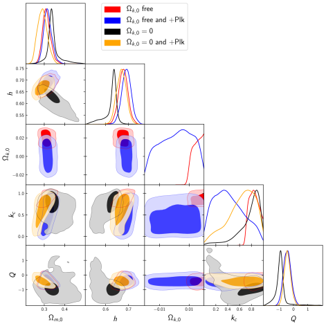
The results of the parameter inference procedure can be found in Fig. 3: the marginalized posteriors for the parameters; along with Table 1. For best-fit values (last row of the table), with their 1$\sigma$, we have: $\Omega_{\rm m}=0.315\pm 0.053$, $h=0.699\pm 0.012$, $\Omega_{\rm k}=0.017\pm 0.002$, $k_{c}=0.83\pm 0.09$ and $Q=-0.67\pm 0.12$. To compare how the CMaDE model performs we assess the fitness to the data via $-2\Delta\ln\mathcal{L_{\rm max}}=-2\ln\mathcal{L_{\rm max,LCDM}}+2\ln\mathcal{L_{\rm max,CMaDE}}$, which is the difference between our model’s best-fit to the data versus $\Lambda$CDM’s; and the Bayes’ Factor $B_{1,2}=E_{1}/E_{2}$, or, more specifically, its natural logarithm $\ln{B_{1,2}}$ where $E_{i}$ is the Bayesian Evidence for a model $i$. In this study we obtained $-2\Delta\ln\mathcal{L_{\rm max}}=3.65$ in favour of the CMaDE model, indicating a better fitness to the data used. The Bayes’ factor obtained is $\ln{B_{1,2}}=2.3$, indicating that CMaDE is in a slight disadvantage (almost moderate evidence) against the standard model when explaining the observations according to the empirical Jeffrey’s Scale in Table 2 following the convention from Trotta:2008qt . This is not unexpected given that our model has two extra parameters and the Bayesian Evidence penalizes the added complexity.

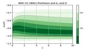
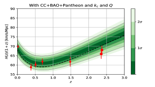
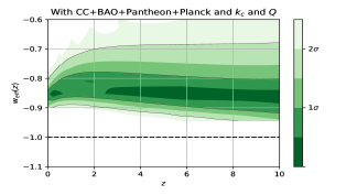
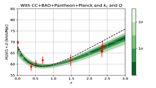
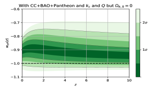
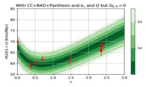
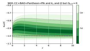
On the other hand, in Figure 2 we observe the functional posteriors for CMaDE’s EoS and the Hubble Parameter $H(z)/(1+z)$. The effective EoSs present Quintessence-like behaviour, and as we go further into the past, CMaDE’s EoS starts resembling that of LCDM as expected. The deviation of CMaDE’s Hubble Parameter from the standard model is significant enough so that it fits better the BAO data at $z\approx 2.35$. We consider this a positive indication for our model since, despite possessing a distinct theoretical foundation and dynamic behavior in the equation of state, our model yields characteristics that closely resemble those of the standard model and even explains better some observations.

Table 1: Mean values, and standard deviations, for the parameters used throughout the reconstructions. For each model, the last two columns present the Bayes Factor, and the $-2\Delta\ln\mathcal{L_{\rm max}}\equiv-2\ln(\mathcal{L_{\rm max}}_{,\Lambda\text{CDM}}/\mathcal{L_{\rm max,}}_{i}$) for fitness comparison. Here $-2\ln\mathcal{L_{\rm max}}_{,\Lambda\text{CDM}}=1429.71$, $\ln E_{\Lambda\text{CDM}}=-721.59(0.14)$ when not including the Planck data set and $-2\ln\mathcal{L_{\rm max}}_{,\Lambda\text{CDM}}=1431.4$, $\ln E_{\Lambda\text{CDM}}=-726.16(0.14)$ when including it.

Model	$h$	$\Omega_{0\rm m}$	$\Omega_{0\rm k}$	$\ln B_{\Lambda\text{CDM},i}$	$-2\Delta\ln\mathcal{L_{\rm max}}$
$\Lambda$CDM	0.694 (0.016)	0.311 (0.012)	–	0	0
CMaDE $\Omega_{0\rm k}=0$	0.646 (0.029)	0.335 (0.058)	–	0.83 (0.21)	3.21
CMaDE	0.683 (0.014)	0.311 (0.065)	0.001 (0.011)	0.10 (0.19)	3.25
With Planck data
$\Lambda$CDM	0.682 (0.008)	0.302 (0.011)	–	0	0
CMaDE $\Omega_{0\rm k}=0$	0.685 (0.019)	0.301 (0.051)	–	2.15 (0.21)	1.35
CMaDE	0.699 (0.012)	0.315 (0.053)	0.017 (0.002)	2.3 (0.21)	3.65

Table 2: Jeffreys’ scale for model selection.

$\ln{B_{12}}$	Odds	Probability	Strength of evidence
$<$ 1.0	$<$3:1	$<$0.75	Inconclusive
1.0	$\sim$3:1	0.750	Weak evidence
2.5	$\sim$12:1	0.923	Moderate evidence
5.0	$\sim$150:1	0.993	Strong evidence

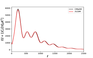
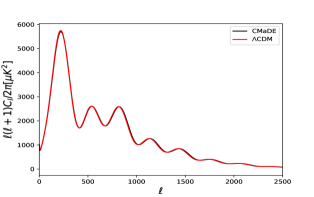
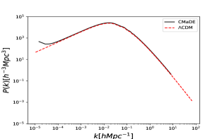
For the comparison of the CMaDE model with CMB and MPS we use the CLASS code Lesgourgues:2011re ; Matos:2021jef ; Lesgourgues:2011rg ; Lesgourgues:2011rh , with the preferred values for $k_{c}=0.42$ and $Q=-0.43$ and we use an approximation similar to the one in Matos:2022jzf . With this modification to the code, we generate Fig. 4 whose best fit corresponds to $H_{0}=68$ km/s/Mpc, $\Omega_{0\rm b}=0.048$, $\Omega_{0DM}=0.23$ and $\Omega_{0\rm k}=0.001$. We see a very good coincidence with the best fit to the CMB and MPS of $\Lambda$CDM and consistency with the values of the previous results.

IV Conclusions

In this work we follow the idea of the reference Matos:2021jef where the space-time fluctuations produced by the big bang are incorporated into Einstein’s equations. The Einstein’s equations (1) contain an extra term $2\pi^{2}/{\lambda}^{2}$ that incorporates the energy of these fluctuations in space-time if ${\lambda}$ is the Compton wavelength of the graviton. In Matos:2021jef it was found that these fluctuations can explain the accelerated expansion of the universe and in Matos:2022jzf it was shown that these fluctuations represented in this new term in Einstein’s equations are in agreement with the main observations of cosmology profiles of MPS and CMB. Note that the CMaDE model does not use an alternative theory of gravity, the only difference of the equations (1) with Einstein’s originals is the term $2\pi^{2}/{\lambda}^{2}$, which is a consequence of GWB fluctuations in space-time. We can interpret this extra term as the contribution of the GWB produced by the big bang to the energy of the universe. In the present work we do not use the approximation ${T^{\mu\nu}}_{;\nu}=0$ to eliminate the small violation of the covariance principle, without this approximation we show that the agreement between the observations of CC, BAO and Pantheon is in favor with the CMaDE model, with $\Delta\chi^{2}=3.65$ over $\Lambda$CDM. In addition, we compare the CMaDE model with the CMB and MPS and we observe that the fit is again in agreement by using the values for the free constants of the model, reducing the so-called tension $H_{0}$. The final conclusion is that the accelerated expansion of the universe can be explained taking into account the GWB energy of space-time, without cosmological constant or modifications of Einstein’s equations.

References

- (1) T. Matos and L. L-Parrilla, “The graviton Compton mass as Dark Energy,” Rev. Mex. Fis., vol. 67, no. 4, p. 040703, 2021.
- (2) V. Poulin, T. L. Smith, and T. Karwal, “The ups and downs of early dark energy solutions to the hubble tension: a review of models, hints and constraints circa 2023,” arXiv preprint arXiv:2302.09032, 2 2023.
- (3) K. Bamba, “Review on Dark Energy Problem and Modified Gravity Theories,” LHEP, vol. 2022, p. 352, 2022.
- (4) N. Frusciante and L. Perenon, “Effective field theory of dark energy: A review,” Phys. Rept., vol. 857, pp. 1–63, 2020.
- (5) G. Agazie et al., “The NANOGrav 15 yr Data Set: Evidence for a Gravitational-wave Background,” Astrophys. J. Lett., vol. 951, no. 1, p. L8, 2023.
- (6) D. J. Reardon et al., “Search for an Isotropic Gravitational-wave Background with the Parkes Pulsar Timing Array,” Astrophys. J. Lett., vol. 951, no. 1, p. L6, 2023.
- (7) H. Xu et al., “Searching for the Nano-Hertz Stochastic Gravitational Wave Background with the Chinese Pulsar Timing Array Data Release I,” Res. Astron. Astrophys., vol. 23, no. 7, p. 075024, 2023.
- (8) J. Antoniadis et al., “The second data release from the European Pulsar Timing Array I. The dataset and timing analysis,” arXiv preprint arXiv:2306.16224, 6 2023.
- (9) E. S. Escobar-Aguilar, T. Matos, and J. I. Jimenez-Aquino, “On the physics of the Gravitational Wave Background,” arXiv preprint arXiv:2303.07111, 3 2023.
- (10) M. Li, “A Model of holographic dark energy,” Phys. Lett. B, vol. 603, p. 1, 2004.
- (11) R.-G. Cai, “A Dark Energy Model Characterized by the Age of the Universe,” Phys. Lett. B, vol. 657, pp. 228–231, 2007.
- (12) T. Matos and L. O. Tellez-Tovar, “The cosmic microwave background and mass power spectrum profiles for a novel and efficient model of dark energy,” Rev. Mex. Fis., vol. 68, no. 2, p. 020705, 2022.
- (13) A. Slosar and J. A. Vazquez. https://github.com/ja-vazquez/SimpleMC.
- (14) E. Aubourg et al., “Cosmological implications of baryon acoustic oscillation measurements,” Phys. Rev. D, vol. 92, no. 12, p. 123516, 2015.
- (15) J. S. Speagle, “dynesty: a dynamic nested sampling package for estimating Bayesian posteriors and evidences,” Mon. Not. Roy. Astron. Soc., vol. 493, no. 3, pp. 3132–3158, 2020.
- (16) S. Alam, M. Ata, S. Bailey, F. Beutler, D. Bizyaev, J. A. Blazek, A. S. Bolton, J. R. Brownstein, A. Burden, C.-H. Chuang, et al., “The clustering of galaxies in the completed SDSS-III Baryon Oscillation Spectroscopic Survey: cosmological analysis of the DR12 galaxy sample,” Mon. Not. Roy. Astron. Soc., vol. 470, no. 3, pp. 2617–2652, 2017.
- (17) V. de Sainte Agathe, C. Balland, H. du Mas des Bourboux, M. Blomqvist, J. Guy, J. Rich, A. Font-Ribera, M. M. Pieri, J. E. Bautista, K. Dawson, et al., “The Extended Baryon Oscillation Spectroscopic Survey: Measuring the Cross-correlation between the MgII Flux Transmission Field and Quasars and Galaxies at ,” Astrophys. J., vol. 878, no. 1, p. 47, 2019.
- (18) M. Ata, F. Baumgarten, J. Bautista, F. Beutler, D. Bizyaev, M. R. Blanton, J. A. Blazek, A. S. Bolton, J. Brinkmann, J. R. Brownstein, et al., “The clustering of the SDSS-IV extended Baryon Oscillation Spectroscopic Survey DR14 quasar sample: first measurement of baryon acoustic oscillations between redshift 0.8 and 2.2,” Mon. Not. Roy. Astron. Soc., vol. 473, no. 4, pp. 4773–4794, 2018.
- (19) M. Blomqvist, H. d. M. d. Bourboux, N. G. Busca, V. d. S. Agathe, J. Rich, C. Balland, J. E. Bautista, K. Dawson, A. Font-Ribera, J. Guy, et al., “Baryon acoustic oscillations from the cross-correlation of lyman- absorption and quasars in eboss dr14,” arXiv preprint arXiv:1904.03430, 2019.
- (20) F. Beutler, C. Blake, M. Colless, D. H. Jones, L. Staveley-Smith, L. Campbell, Q. Parker, W. Saunders, and F. Watson, “The 6dF Galaxy Survey: Baryon Acoustic Oscillations and the Local Hubble Constant,” Mon. Not. Roy. Astron. Soc., vol. 416, pp. 3017–3032, 2011.
- (21) S. Alam et al., “Completed SDSS-IV extended Baryon Oscillation Spectroscopic Survey: Cosmological implications from two decades of spectroscopic surveys at the Apache Point Observatory,” Phys. Rev. D, vol. 103, no. 8, p. 083533, 2021.
- (22) D. Scolnic et al., “The Pantheon+ Analysis: The Full Data Set and Light-curve Release,” Astrophys. J., vol. 938, no. 2, p. 113, 2022.
- (23) M. Moresco. https://gitlab.com/mmoresco/CCcovariance.
- (24) R. Trotta, “Bayes in the sky: Bayesian inference and model selection in cosmology,” Contemp. Phys., vol. 49, pp. 71–104, 2008.
- (25) J. Lesgourgues, “The Cosmic Linear Anisotropy Solving System (CLASS) I: Overview,” arXiv preprint arXiv:1104.2932, 4 2011.
- (26) J. Lesgourgues, “The cosmic linear anisotropy solving system (class) iii: Comparision with camb for lambdacdm,” arXiv preprint arXiv:1104.2934, 4 2011.
- (27) J. Lesgourgues and T. Tram, “The Cosmic Linear Anisotropy Solving System (CLASS) IV: efficient implementation of non-cold relics,” JCAP, vol. 09, p. 032, 2011.