vSHARP: variable Splitting Half-quadratic Admm algorithm for Reconstruction of inverse-Problems

Abstract

Medical Imaging (MI) tasks, such as accelerated Parallel Magnetic Resonance Imaging (MRI), often involve reconstructing an image from noisy or incomplete measurements. This amounts to solving ill-posed inverse problems, where a satisfactory closed-form analytical solution is not available. Traditional methods such as Compressed Sensing (CS) in MRI reconstruction can be time-consuming or prone to obtaining low-fidelity images. Recently, a plethora of supervised and self-supervised Deep Learning (DL) approaches have demonstrated superior performance in inverse-problem solving, surpassing conventional methods. In this study, we propose vSHARP (variable Splitting Half-quadratic ADMM algorithm for Reconstruction of inverse Problems), a novel DL-based method for solving ill-posed inverse problems arising in MI. vSHARP utilizes the Half-Quadratic Variable Splitting method and employs the Alternating Direction Method of Multipliers (ADMM) to unroll the optimization process. For data consistency, vSHARP unrolls a differentiable gradient descent process in the image domain, while a DL-based denoiser, such as a U-Net architecture, is applied to enhance image quality. vSHARP also employs a dilated-convolution DL-based model to predict the Lagrange multipliers for the ADMM initialization. We evaluate the proposed model by applying it to the task of accelerated Parallel MRI Reconstruction on two distinct datasets. We present a comparative analysis of our experimental results with state-of-the-art approaches, highlighting the superior performance of vSHARP.

Keywords Medical Imaging Reconstruction, Inverse Problems, Deep MRI Reconstruction, Mathematical Optimization, Half-Quadratic Variable Splitting, Alternating direction method of multipliers

1 Introduction

Medical Imaging (MI) possesses a wide range of modalities that can by employed in the clinic that can assist in diagnosis, treatment, and treatment planning of patients. The need to acquire high-quality images in a timely manner has been a driving force behind many medical advancements. Inverse problems play a pivotal role in this pursuit, providing a framework to reconstruct accurate images from the limited and often noisy measurements obtained through imaging modalities such as Magnetic Resonance Imaging (MRI). These inverse problems have been the focal point of intensive research, as they lie at the intersection of mathematical modeling, signal processing, and MI.

Traditionally, solving inverse problems arising in MI has relied on well-established mathematical techniques and iterative numerical algorithms. These methods involve imposing prior knowledge about the imaging process, such as sparsity or smoothness constraints, to regularize the ill-posed nature of the problem. In the context of accelerated parallel MRI reconstruction, for instance, techniques like Compressed Sensing (CS) have been employed to recover high-resolution images from undersampled $k$-space data [1].

Recent years have witnessed a transformative shift in the field of medical imaging, largely driven by advancements in the realms of Deep Learning (DL) and Computer Vision. DL-based techniques, particularly convolutional neural networks (CNNs), have shown remarkable potential in solving a diverse range of inverse problems [2, 3, 4]. These methods leverage the capacity of CNNs to learn complex relationships directly from data, eliminating the need for hand-crafted mathematical models and heuristics. This shift has enabled the development of innovative solutions that surpass the limitations of traditional methods in MI. By leveraging large datasets, DL-based reconstruction methods can solve inverse problems by learning complex image representations and effectively reconstruct high-fidelity images, often in a supervised learning (SL) settings [5, 6, 7, 8, 9, 10, 11] or in self-supervised settings [12, 13].

In this study, we propose vSHARP (variable Splitting Half-quadratic ADMM algorithm for Reconstruction of inverse-Problems), an innovative approach to solving inverse problems in Medical Imaging using Deep Learning. The vSHARP method leverages the Half-Quadratic Variable Splitting (HQVS) [14] method and integrates the Alternating Direction Method of Multipliers (ADMM) [15] to unroll an optimization process. By combining a differentiable gradient descent process in the image domain for data consistency and a DL-based denoiser, such as a U-Net [16] or a U-Former [17] architecture, for image enhancement, in addition to utilizing a trained initializer for the ADMM Lagrange multipliers, vSHARP aims to achieve high-quality reconstructions.

To evaluate the performance of vSHARP, we conducted comprehensive experiments focused on accelerated parallel MRI reconstruction and applied vSHARP to two distinct datasets, the Calgary Campinas brain [18] and fastMRI T2 prostate datasets [19].

Our main contributions can be summarized as follows:

• We propose the vSHARP algorithm, a novel versatile DL-based inverse problem solver that can be applied on inverse problems arising in (Medical) Imaging with well-defined forward and adjoint operators.

• We provide a comprehensive mathematical derivation of vSHARP using the general formulation of inverse problems and employing the HQVS and ADMM methods.

• We assess vSHARP’s performance in the context of accelerated parallel MRI reconstruction, utilizing brain and prostate MRI datasets alongside two different sub-sampling schemes. Our results demonstrate vSHARP’s exceptional capabilities, surpassing current baseline methods.

2 Theoretical Background

In imaging, the concept of an inverse problem involves the task of recovering an underlying image $\mathbf{x}\in\mathcal{X}$ from given noisy or incomplete measurements $\tilde{\mathbf{y}}\in\mathcal{Y}$, where $\mathcal{X},\mathcal{Y}$ are Hilbert spaces, with $\mathcal{X}$ representing the space of possible images and $\mathcal{Y}$ representing the space of measurement acquisitions. These measurements, obtained through a known process known as the forward model, are related according to the equation

$$\tilde{\mathbf{y}}=\mathcal{A}\left(\mathbf{x}\right)+\boldsymbol{\epsilon},$$ (1)

where $\mathcal{A}:\mathcal{X}\rightarrow\mathcal{Y}$ denotes the forward measurement operator. Here we assume that $\boldsymbol{\epsilon}\sim\mathcal{N}(\boldsymbol{0},\mathbf{I}_{\mathcal{Y}})$ represents additive measurement noise, although this might not be the case for some inverse problems. The operator $\mathcal{A}$, known as the forward operator, is often a composition of various processes, such as blurring, subsampling, sensor sensitivity, and others, depending on the specific problem.

The adjoint [20] operator of $\mathcal{A}$ is denoted as $\mathcal{A}^{*}:\mathcal{Y}\rightarrow\mathcal{X}$ and is defined as the unique linear operator such that

$$\left<\mathcal{A}\left(\mathbf{x}\right),\,\mathbf{y}\right>_{\mathcal{Y}}\,=\,\left<\mathbf{x},\,\mathcal{A}^{*}\left(\mathbf{y}\right)\right>_{\mathcal{X}},\quad\forall\mathbf{x}\in\mathcal{X},\,\mathbf{y}\in\mathcal{Y},$$ (2)

where $\left<\cdot,\cdot\right>_{\mathcal{X}},\left<\cdot,\cdot\right>_{\mathcal{Y}}$ are inner products on $\mathcal{X},\mathcal{Y}$ respectively. The adjoint operator is easy to evaluate for modalities such as Magnetic Resonance Imaging and Computed Tomography, and it allows us to reconstruct an image from observed measurements as $\mathcal{A}^{*}\left(\tilde{\mathbf{y}}\right)$. However, $\mathcal{A}^{*}$ is not necessarily equal to the inverse $\mathcal{A}^{-1}$ of $\mathcal{A}$, even when $\mathcal{A}$ is invertible. In general, due to the noise $\boldsymbol{\epsilon}$ introduced by the measurement process and the fact that $\mathcal{A}$ might have nontrivial kernel (e.g. in accelerated MRI or sparse-view CT), the problem stated in (1) becomes ill-posed [21].

Instead of trying derive an analytical approximation to $\mathcal{A}^{-1}$ to arrive at an approximate reconstruction of $\mathbf{x}$, a common approach is to formulate and solve a regularized least squares optimization problem, combining data fidelity and regularization terms:

$$\mathbf{x}^{*}=\operatorname*{argmin}_{\mathbf{x}\in\mathcal{X}}\left|\left|\mathcal{A}(\mathbf{x})-\mathbf{y}\right|\right|_{2}^{2}+\lambda\mathcal{R}(\mathbf{x}).$$ (3)

Here, the regularization functional $\mathcal{R}:\mathcal{X}\rightarrow\mathbb{R}$ encodes prior knowledge about the underlying image, and $\lambda>0$ controls the trade-off between data fidelity and regularization strength. Solving this optimization problem entails employing numerical techniques, often iterative algorithms that alternate between forward and adjoint operations, aiming to converge towards a solution that effectively balances measurement fidelity and adherence to prior image information.

Common optimization methods for solving (3) include gradient-based techniques like Gradient Descent, Proximal Gradient [22], and Conjugate Gradient [23]. More sophisticated algorithms such as ADMM [24] and Primal-Dual hybrid gradient [25] are also utilized. In this work, we propose an approach that combines the Half-Quadratic Variable Splitting algorithm with an Alternating Direction Method of Multipliers formulation.

2.1 Variable Half-quadratic Splitting

We employ the HQVS method [14] by first introducing an auxiliary variable $\mathbf{z}\in\mathcal{X}$ and reformulating (3) in the following equivalent form:

$$\mathbf{x}^{*}=\operatorname*{argmin}_{\mathbf{x}\in\,\mathcal{X}}\left(\min_{\mathbf{z}\in\mathcal{X},\mathbf{z}-\mathbf{x}=0}\,\frac{1}{2}\big{|}\big{|}\mathcal{A}\left(\mathbf{x}\right)-\tilde{\mathbf{y}}\big{|}\big{|}_{2}^{2}+\lambda\,\mathcal{R}(\mathbf{z})\right).$$ (4)

This constrained optimization problem can be solved by applying the augmented Lagrangian method [26], i.e.,

$$\mathbf{x}^{*}=\operatorname*{argmin}_{\mathbf{x}\in\mathcal{X}}\left(\min_{\mathbf{z}\in\mathcal{X}}\max_{\mathbf{u}\in\mathcal{X}}\mathcal{L}_{\rho}(\mathbf{x},\mathbf{z},\mathbf{u})\right),$$ (5)

where $\mathcal{L}_{\rho}$ denotes the augmented Lagrangian for (4), defined as:

$$\mathcal{L}_{\rho}(\mathbf{x},\mathbf{z},\mathbf{u})=\frac{1}{2}\big{|}\big{|}\mathcal{A}(\mathbf{x})-\tilde{\mathbf{y}}\big{|}\big{|}_{2}^{2}+\lambda\,\mathcal{R}(\mathbf{z})+\left<\mathbf{u},\mathbf{x}-\mathbf{z}\right>_{\mathbb{X}}+\frac{\rho}{2}\big{|}\big{|}\mathbf{x}-\mathbf{z}\big{|}\big{|}_{2}^{2},$$ (6)

where $\mathbf{u}$ denotes the Lagrange multipliers and $\rho>0$ is a penalty parameter.

2.2 Unrolling via ADMM

Equation 4 can be iteratively solved over $T$ iterations by applying the ADMM algorithm which comprises the following updates:

$$\mathbf{z}^{t+1}=\operatorname*{argmin}_{\mathbf{z}\in\mathcal{X}}\,\lambda\,\mathcal{R}(\mathbf{z})+\frac{{\rho}_{t+1}}{2}\big{|}\big{|}\mathbf{x}^{t}-\mathbf{z}+\frac{\mathbf{u}^{t}}{{\rho}_{t+1}}\big{|}\big{|}_{2}^{2}\quad\quad\text{{[z-step]}}$$ (7a)

$$\mathbf{x}^{t+1}=\operatorname*{argmin}_{\mathbf{x}\in\mathcal{X}}\,\frac{1}{2}\big{|}\big{|}\mathcal{A}(\mathbf{x})-\tilde{\mathbf{y}}\big{|}\big{|}_{2}^{2}+\frac{{\rho}_{t+1}}{2}\big{|}\big{|}\mathbf{x}-\mathbf{z}^{t+1}+\frac{\mathbf{u}^{t}}{{\rho}_{t+1}}\big{|}\big{|}_{2}^{2}\quad\quad\text{{[x-step]}}$$ (7b)

$$\mathbf{u}^{t+1}=\mathbf{u}^{t}+{\rho}_{t+1}(\mathbf{x}^{t+1}-\mathbf{z}^{t+1})\quad\quad\text{{[u-step]}}$$ (7c)

where $0\,\leq\,t\,\leq\,T-1$ denotes the iteration index. In Appendix A we provide analytically the ADMM algorithm as well as a more detailed derivation of (7c). Note that instead of using a single penalty parameter for all iterations, we employ a varying penalty parameter per iteration: $\boldsymbol{\rho}=(\rho_{1},\,\rho_{2},\cdots,\,\rho_{T})\in(\mathbb{R}^{+})^{T}$.

3 Methods

3.1 From Unrolled ADMM to vSHARP

In this section, we introduce the variable Splitting Half-quadratic Algorithm for Reconstruction of inverse-Problems (vSHARP) network. vSHARP is a DL-based approach designed to solve (7c).

At iteration $t$, vSHARP addresses the $\mathbf{z}$-step in (7a) by learning a representation of $\mathbf{z}^{t+1}$ based on $\mathbf{z}^{t}$, $\mathbf{x}^{t}$, and $\mathbf{u}^{t}$, using a deep neural network denoiser $\mathcal{R}_{{\boldsymbol{\theta}}_{t}}$ with trainable parameters ${\boldsymbol{\theta}}_{t}$:

$$\mathbf{z}^{t+1}\,=\,\mathcal{R}_{{\boldsymbol{\theta}}_{t+1}}(\mathbf{z}^{t},\,\mathbf{x}^{t},\,\frac{\mathbf{u}^{t}}{{\rho}_{t+1}}).$$ (8)

Options for $\mathcal{R}_{{\boldsymbol{\theta}}_{t}}$ include architectural choices such as U-Nets, U-Formers, or other Deep Learning-based (convolutional) structures like ResNet [27], DIDN [28], or simple convolution blocks.

Moving on to the $\mathbf{x}$-step in (7b), the closed-form solution can be expressed as

$$\mathbf{x}^{t+1}\,=\,\big{(}\mathcal{A}^{*}\circ\mathcal{A}\,+\,{\rho}_{t+1}\mathbf{I}_{n}\big{)}^{-1}\big{(}\mathcal{A}^{*}(\tilde{\mathbf{y}})\,+\,{\rho}_{t+1}\,\mathbf{z}^{t+1}\,-\,\mathbf{u}^{t}\big{)}.$$ (9)

However, in practice, computing the operator $\big{(}\mathcal{A}^{*}\circ\mathcal{A}\,+\,{\rho}_{t+1}\mathbf{I}_{n}\big{)}^{-1}$ can be computationally intensive or even infeasible. To address this, vSHARP unrolls (7b) in $T_{\mathbf{x}}$ steps using Data Consistency via Gradient Descent (DCGD), a differentiable Gradient Descent scheme, as outlined by Algorithm 1, with step sizes $\boldsymbol{\eta}\in(\mathbb{R}^{+})^{T_{\mathbf{x}}}$.

1

2Input:
$\rho>0$, $T_{x}>0$, step sizes $\boldsymbol{\eta}$ ;
From current iteration: $\mathbf{z}^{t+1}$ ;
From previous iteration: $\mathbf{x}^{t}$, $\mathbf{u}^{t}$ ;

3Set $\mathbf{w}^{0}\,=\,\mathbf{x}^{t}$ ;

4for $s\,=\,0$ to $T_{x}-1$ do

5       Calculate gradient update: $\mathbf{\nabla}_{\mathbf{w}}^{s+1}\,=\,\mathcal{A}^{*}\Big{(}\mathcal{A}(\mathbf{w}^{s})\,-\tilde{\mathbf{y}}\Big{)}\,+\,\rho\,\Big{(}\mathbf{w}^{s}\,-\,\mathbf{z}^{t+1}\,+\,\frac{\mathbf{u}^{t}}{\rho}\Big{)}$ ;

6      Update $\mathbf{w}^{s+1}\,=\,\mathbf{w}^{s}\,-\,\eta_{s+1}\,\mathbf{\nabla}_{\mathbf{w}}^{s+1}$ ;

7

8Set $\mathbf{x}^{t+1}\,=\,\mathbf{w}^{T_{x}}$ ;

Output: $\mathbf{x}^{t+1}$ ;

Algorithm 1 $\mathbf{x}$-step: Data Consistency via Gradient Descent (DCGD)

Lastly, the $\mathbf{u}$-step in Equation 7c is straightforward as described by (7c). This step updates the Lagrange multipliers based on the difference between the current estimates of $\mathbf{x}$ and $\mathbf{z}$. The parameter ${\rho}_{t+1}$ controls the step size of the update.

3.2 Initialization of Variables and Parameters of vSHARP

Proper initialization of the image $\mathbf{x}^{0}$, auxiliary variable $\mathbf{z}^{0}$, and Lagrange multiplier $\mathbf{u}^{0}$ can enhance the convergence of the ADMM algorithm and promote better reconstruction outcomes.

3.2.1 Image and Auxiliary Variable Initialization

A reasonable initialization for $\mathbf{x}^{0}$ and $\mathbf{z}^{0}$ can be produced by using the observed measurements $\tilde{\mathbf{y}}$, for instance:

$$\mathbf{x}^{0},\,\mathbf{z}^{0}\,=\,\mathcal{A}^{*}\left(\tilde{\mathbf{y}}\right),$$ (10)

although different task-specific initializations can be used.

3.2.2 Lagrange Multipliers Initialization

In our framework, the initialization of the Lagrange multiplier $\mathbf{u}^{0}$ involves the use of a neural network $\mathcal{G}_{\boldsymbol{\psi}}$ with trainable parameters $\boldsymbol{\psi}$:

$$\mathbf{u}^{0}=\mathcal{G}_{\boldsymbol{\psi}}\left(\mathbf{x}^{0}\right).$$ (11)

The purpose of this network is to provide an initial estimation of the Lagrange multipliers based on the initial image guess $\mathbf{x}^{0}$. The architecture of the Lagrange multiplier initializer model draws inspiration from previous works, specifically the replication padding (ReplicationPadding) module [29] and dilated convolutions [30]. The model consists of four layers of replication padding followed by a two-dimensional dilated convolution with a specified dilation factor and filter size. The output of this convolutional layer is then passed through a series of two-dimensional $1\times 1$ convolutions, followed by a rectified linear unit (ReLU) activation function.

By incorporating these initialization steps, vSHARP sets the initial values of $\mathbf{x}$, $\mathbf{z}$, and $\mathbf{u}$, enabling the iterative reconstruction process to begin from a reasonable starting point.

3.2.3 Initialization of Optimization Parameters

Instead of making the penalty $\boldsymbol{\rho}$ a hyper-parameter, its chosen as a trainable parameter of vSHARP and it is initialized from the truncated normal distribution $\mathcal{N}_{\text{trunc}}(0,\,\mathbf{I}_{T})$. Furthermore, vSHARP also learns the values of the step sizes $\boldsymbol{\eta}$ for the DCGD step, which is also initialized from $\mathcal{N}_{\text{trunc}}(0,\,\mathbf{I}_{T_{x}})$.

3.3 End-to-end Pipeline of vSHARP

1

2Input:
$T\,>\,0,\,T_{\mathbf{x}}\,>\,0$, $\boldsymbol{{\rho}}\in\mathbb{R}^{T}$, $\boldsymbol{\eta}\in\mathbb{C}^{T_{\mathbf{x}}}$ ;

3Initialize:
$\mathbf{x}^{0}\,=\,\mathcal{A}^{*}(\tilde{\mathbf{y}})$ ;
$\mathbf{z}^{0}\,=\,\mathbf{x}^{0}$ ;
$\mathbf{u}^{0}\,=\,\mathcal{G}_{\boldsymbol{\psi}}(\mathbf{x}^{0})$ ;

4for $t\,=\,0$ to $T-1$ do

       Update $\mathbf{z}^{t+1}\,=\,\mathcal{R}_{\theta_{t+1}}(\mathbf{z}^{t},\,\mathbf{x}^{t},\,\frac{\mathbf{u}^{t}}{{\rho}_{t+1}})$ ;

        // $\mathcal{R}_{\theta_{t}}$ denoiser at $t$-th step

5      

6      

      Update $\mathbf{x}^{t+1}\,=\,\text{DCGC}_{({\rho}_{t+1},T_{x},\boldsymbol{\eta})}(\mathbf{z}^{t+1},\,\mathbf{x}^{t},\,\mathbf{u}_{t})$ ;

        // Data Consistency via Gradient Descent

7      

8      

9      Update $\mathbf{u}^{t+1}=\mathbf{u}^{t}+{\rho}_{t+1}(\mathbf{x}^{t+1}-\mathbf{z}^{t+1})$ ;

10

11

12Output: $\left\{\mathbf{x}^{t}\right\}_{t=1}^{T}$ ;

Algorithm 2 vSHARP: variable Splitting Half-quadratic ADMM algorithm for Reconstruction of inverse-Problems

The complete vSHARP reconstruction process follows a systematic pipeline, leveraging the strategies outlined in the previous sections. Algorithm 2, combines all aforementioned strategies and outlines the end-to-end vSHARP pipeline. We also provide a graphical illustration of the end-to-end pipeline in Fig. 1.

At each iteration, vSHARP refines the estimates of $\mathbf{x}$, $\mathbf{z}$, and $\mathbf{u}$, moving closer to an accurate reconstruction. vSHARP outputs a sequence of reconstructions obtained at all optimization time-steps $\left\{\mathbf{x}^{t}\right\}_{t=1}^{T}$. Although $\mathbf{x}^{*}=\mathbf{x}_{T}$ is the prediction of the underlying image, all time-step predictions can be used for the loss computation in Section 3.4 to train the model.

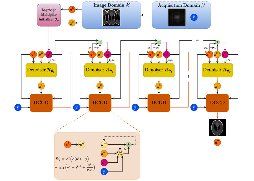
Figure 1: Graphical Illustration of vSHARP. Utilizing acquired measurements $\tilde{\mathbf{y}}$ from the acquisition domain $\mathcal{Y}$, initial estimations are made for the image $\mathbf{x}_{0}$ and the auxiliary variable $\mathbf{z}_{0}$ (in the image domain $\mathcal{X}$. The Lagrange Multiplier Initializer Network $\mathcal{G}_{\boldsymbol{\psi}}$ [6] generates an initialization $\mathbf{u}_{0}$ for the Lagrange multipliers, using $\mathbf{x}_{0}$ as input. These images, namely $\mathbf{z}_{0}$, $\mathbf{x}_{0}$, and $\mathbf{u}_{0}$, serve as the initial quantities in the unrolled ADMM algorithm spanning $T$ iterations. During each iteration, a DL-based denoiser $\mathcal{R}_{\boldsymbol{\theta}_{t}}$ (in this case, a U-Net) is employed to refine $\mathbf{z}_{t}$, while $\mathbf{x}_{t}$ undergoes optimization through a differentiable Data Consistency via Gradient Descent (DCGD) algorithm. The DCGD algorithm itself is further unrolled over $T_{\mathbf{x}}$ iterations. As the result of these operations, vSHARP produces $\mathbf{x}_{T}$ as the predicted reconstructed image.

In our experimental setup (Section 4), we particularize vSHARP for an ill-posed inverse problem, specifically accelerated parallel MRI reconstruction.

3.4 vSHARP Training

Let $\mathbf{x}$ be the ground truth image, $\mathbf{y}$ and $\left\{\mathbf{y}^{t}\right\}_{t=1}^{T}$ the corresponding ground truth and predicted measurements (obtained from the predicted images $\left\{\mathbf{x}^{t}\right\}_{t=1}^{T}$ using some relevant transformation for the specific task). Then, for arbitrary loss functions $\mathcal{L}_{\mathcal{X}}$ and $\mathcal{L}_{\mathcal{Y}}$, computed in the image and measurements domains respectively, vSHARP is trained by computing the following:

$$\mathcal{L}\left(\mathbf{x},\mathbf{x}^{t}\right)=\sum_{t=1}^{T}w_{t}\left[\mathcal{L}_{\mathcal{X}}\left(\mathbf{x},\mathbf{x}^{t}\right)+\mathcal{L}_{\mathcal{Y}}\left(\mathbf{y},\mathbf{y}^{t}\right)\right],\quad w_{t}=10^{\frac{t-T}{T-1}},\quad t=1,\cdots,T$$ (12)

4 Experiments

4.1 Accelerated Parallel MRI Reconstruction

4.1.1 Defining the Problem

In the context of accelerated Parallel MRI Reconstruction, the primary objective is to generate a reconstructed complex image $\mathbf{x}\in\mathcal{X}=\mathbb{C}^{n}$ from undersampled $k$-space data collected from multiple ($n_{c}$) coils, denoted as $\tilde{\mathbf{y}}\in\mathcal{Y}=\mathbb{C}^{n\times n_{c}}$. An essential aspect of parallel MRI involves calculating coil sensitivity maps $\mathbf{C}=(\mathbf{C}_{1},\mathbf{C}_{2},\ldots,\mathbf{C}_{n_{c}})\in\mathbb{C}^{n\times n_{c}}$, which indicate the spatial sensitivity of each individual coil. Typically, these maps are pre-computed from the central region of the multi-coil $k$-space, often referred to as the autocalibration (ACS) region.

The forward operator $\mathcal{A}_{\mathbf{M},\mathbf{C}}:\mathbb{C}^{n}\rightarrow\mathbb{C}^{n\times n_{c}}$ and the adjoint operators $\mathcal{A}_{\mathbf{M},\mathbf{C}}^{*}:\mathbb{C}^{n\times n_{c}}\rightarrow\mathbb{C}^{n}$ for accelerated parallel MRI can be defined as follows:

$$\mathcal{A}_{\mathbf{M},\mathbf{C}}(\mathbf{x})=\mathbf{M}\circ\mathcal{F}\circ\mathcal{E}_{\mathbf{C}}(\mathbf{x}),\quad\mathcal{A}_{\mathbf{M},\mathbf{C}}^{*}=\mathcal{R}_{\mathbf{C}}\circ\mathcal{F}^{-1}\circ\mathbf{M}.$$ (13)

In the forward operator, an undersampling operator $\mathbf{M}$ is combined with the two-dimensional Fourier transform $\mathcal{F}$ and the coil-encoding operator $\mathcal{E}_{\mathbf{C}}:\mathbb{C}^{n}\rightarrow\mathbb{C}^{n\times n_{c}}$, which transforms the image $\mathbf{x}\in\mathbb{C}^{n}$ into separate coil images using $\mathbf{C}$ as shown below:

$$\mathcal{E}_{\mathbf{C}}(\mathbf{x})\,=\,\big{(}\mathbf{C}_{1}\mathbf{x},\,\mathbf{C}_{2}\mathbf{x},\cdots,\,\mathbf{C}_{n_{c}}\mathbf{x}\big{)}.$$ (14)

On the other hand, the adjoint operator performs undersampling on the multi-coil $k$-space data, followed by the two-dimensional inverse Fourier transform $\mathcal{F}^{-1}$, and then applies the SENSE operator $\mathcal{R}_{\mathbf{C}}:\mathbb{C}^{n\times n_{c}}\rightarrow\mathbb{C}^{n}$, which combines individual coil images $\mathbf{z}\in\mathbb{C}^{n\times n_{c}}$ using $\mathbf{C}$:

$$\mathcal{R}_{\mathbf{C}}(\mathbf{z})=\sum_{k=1}^{n_{c}}\mathbf{C}_{k}^{*}\mathbf{z}_{k}.$$ (15)

4.1.2 Estimation and Refinement of Sensitivity Maps

In our experimental framework, we employ the ACS $k$-space data to initially compute $\tilde{\mathbf{C}}$ as an estimation of the sensitivity maps. Subsequently, we employ a deep learning-based model $\mathcal{S}_{\theta_{\mathcal{S}}}$ with trainable parameters $\theta_{\mathcal{S}}$ to refine the sensitivity maps, utilizing $\tilde{\mathbf{C}}$ as input:

$$\mathbf{C}_{k}=\mathcal{S}_{\theta_{\mathcal{S}}}(\tilde{\mathbf{C}}_{k}),\quad k=1,\cdots,n_{c}.$$ (16)

This module is trained end-to-end along with vSHARP.

4.1.3 Experimental Setup

Datasets

In our experimentation, as aforementioned, we utilized two publicly accessible datasets: the Calgary-Campinas (CC) brain dataset released as part of the Multi-Coil MRI Reconstruction (MCMRI) Challenge [18] and the fastMRI T2 prostate dataset [19]. Both datasets consist of fully-sampled, 2D axial, multi-coil k-space measurements. The CC dataset encompasses 67 T1-weighted acquisitions, which we divided into training (40 volumes, 7332 2D slices), validation (10 volumes, 1560 2D slices), and test (10 volumes, 1560 2D slices) subsets. The fastMRI T2 prostate dataset comprises data from 312 subjects, partitioned into training (218 volumes, 6602 2D slices), validation (48 volumes, 1462 2D slices), and test (46 volumes, 1399 2D slices) sets.

Undersampling

In order to comprehensively assess our model’s capabilities, we incorporated the use of distinct undersampling patterns in our experiments.

Given that the available data was fully-sampled, we retrospectively applied undersampling techniques to simulate acceleration factors of 4, 8, and 16. It is noteworthy that for each acceleration factor, we retained an 8%, 4%, and 2% center fraction of the fully-sampled data within the autocalibration region. During the training phase, we applied random undersampling to the data, whereas during the inference phase, we evaluated the model’s performance by undersampling the data across all acceleration levels.

For the CC dataset, we employed Variable Density Poisson disk masks, which were provided along with the dataset. On the other hand, for the fastMRI prostate data, we opted for vertical rectilinear equispaced subsampling [31]. This choice was influenced by the practicality of implementing equispaced subsampling, which closely aligns with standard MRI scanner procedures.

Training Details

Given these conditions, the training of vSHARP was executed utilizing the retrospectively undersampled $k$-space measurements $\tilde{\mathbf{y}}=\mathbf{M}(\mathbf{y})$, where $\mathbf{y}$ represents the fully-sampled $k$-space measurements. A ground truth image $\mathbf{x}$ was obtained from applying the inverse Fourier transform on $\mathbf{y}$ followed by the root-sum-of-squares (RSS) operation:

$$\mathbf{x}=\text{RSS}\circ\mathcal{F}^{-1}(\mathbf{y})=\left(\sum_{k=1}^{n_{c}}|\mathcal{F}^{-1}(\mathbf{y}_{k})|^{2}\right)^{1/2}.$$ (17)

It is worth noting that the RSS method was chosen as it has been demonstrated to be the optimal unbiased estimator for the underlying ground truth image [32].

Furthermore, we initialized (10) as $\mathbf{x}_{0}=\mathbf{z}_{0}=\mathcal{A}_{\mathbf{M},\mathbf{C}}^{*}(\tilde{\mathbf{y}})$.

For the purpose of computing the loss and obtaining predicted $k$-space measurements from the model, we transformed the predicted images from vSHARP $\left\{\mathbf{x}^{t}\right\}_{t=1}^{T}$ to the $k$-space domain using the following transformation:

$$\left\{\mathbf{y}^{t}\right\}_{t=1}^{T}=\left\{\mathcal{F}\circ\mathcal{E}_{\mathbf{C}}\left(\mathbf{x}^{t}\right)\right\}_{t=1}^{T}$$ (18)

We computed a combination of various loss functions with equal weighting computed in both the image and $k$-space domains. To be specific, we formulated the training losses as:

$$\mathcal{L}_{\mathcal{X}}:=\mathcal{L}_{1}+\text{SSIMLoss}+\text{HFEN}_{1}+\text{HFEN}_{2},\quad\mathcal{L}_{\mathcal{Y}}:=\text{NMSE}+\text{NMAE}.$$ (19)

For the aforementioned loss functions, we utilized the loss definitions as described in [31]. In the interest of brevity, we have refrained from providing their explicit delineation here and instead, we refer readers to Appendix Section B.

Model Implementation

For accelerated parallel MRI reconstruction, we designed a vSHARP model with $T=12$ ADMM optimization steps and $T_{\mathbf{x}}=10$ DCGD steps. Within the $\mathbf{z}$-step denoising process, we utilized two-dimensional U-Nets [16] with four scales and initiated the first scale with 32 convolutional filters. For the sensitivity maps refinement, we integrated a U-Net with four scales and 16 filters in the first scale.

5 Experimental Results

5.1 Accelerated Parallel MRI Reconstruction

For our experiments in this section, including the model implementations, datasets handling, and all DL utilities, we employed the DIRECT toolkit [33].

5.1.1 Comparative Analysis

We conducted a comprehensive comparison involving our vSHARP implementation (as detailed in Section 4.1.3), alongside a baseline and two state-of-the-art MRI reconstruction techniques:

1. A U-Net with four scales, where the first scale comprised 64 convolutional filters.

2. An End-to-End Variational Network (E2EVarNet) [34] with 12 cascades and U-Net regularizers, incorporating four scales and initializing the first scale with 64 convolutional filters.

3. A Recurrent Variational Network (RecurrentVarNet) [6], winning solution to the MCMRI Challenge [18], adhering to the architectural specifics outlined in the original publication.

To maintain consistency, a sensitivity map refinement module was incorporated into all approaches using identical hyperparameters as the one integrated with vSHARP.

Training Details

In our experimental setup for accelerated parallel MRI reconstruction, the optimization process for our proposed model and the comparison models was carried out using the Adam optimizer. The optimizer’s hyperparameters were set as follows: $\beta_{1}=0.9$, $\beta_{2}=0.999$, and $\epsilon=1e-8$. The experiments were conducted on separate NVIDIA A6000 GPUs.

For the Calgary-Campinas dataset, the models were trained with a batch size of 2 two-dimensional slices over 100,000 iterations. Similarly, for the FastMRI prostate dataset, models were trained with a batch size of 1 two-dimensional slice for 120,000 iterations.

To initiate training, a warm-up schedule was implemented. This schedule linearly increased the learning rate to its initial value of 0.002 over the course of 1000 warm-up iterations, applied to both datasets.

Subsequently, a learning rate decay strategy was employed during training. Specifically, for the Calgary-Campinas experiment, the learning rate was reduced by a factor of 0.2 every 20,000 training iterations. In contrast, for the FastMRI prostate experiments, the learning rate decay occurred every 30,000 iterations.

Quantitative Results

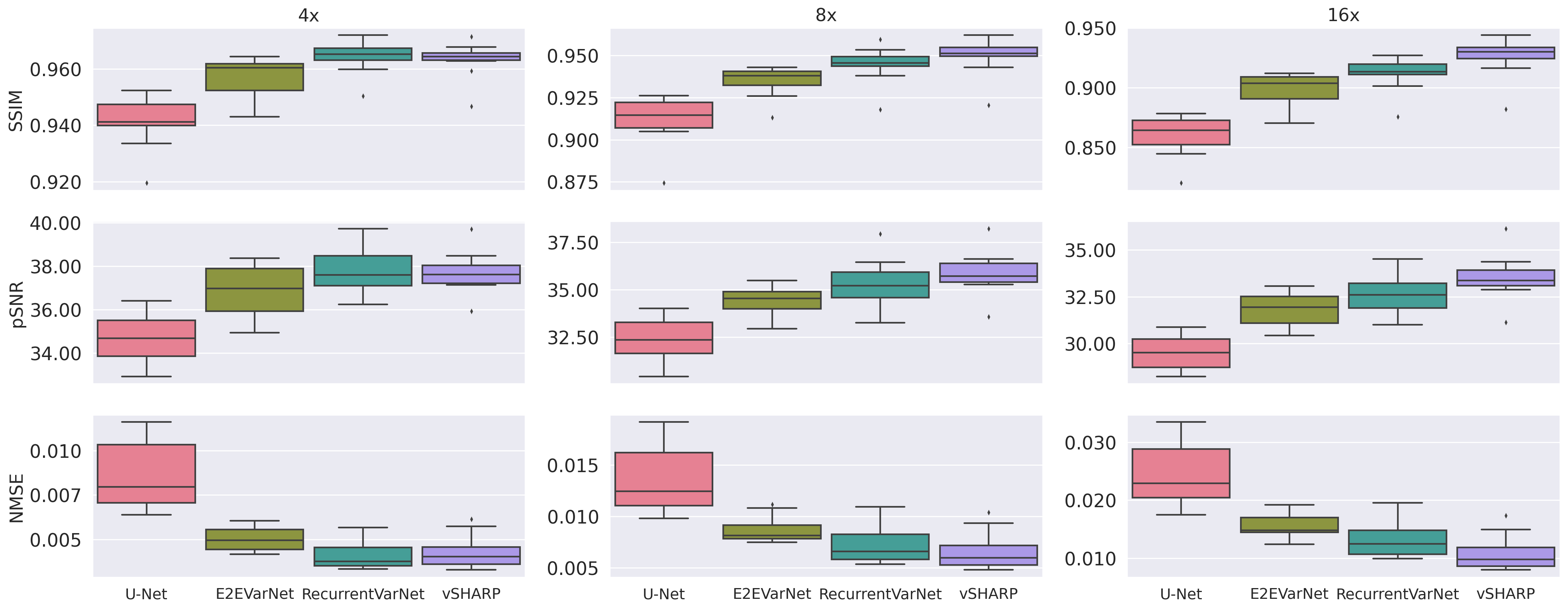
Figure 2: Box Plots illustrating the quantitative results on the Calgary-Campinas test set.

Table 1: Average evaluation metrics on the Calgary-Campinas test set.

Model	Metrics
	$4\times$			$8\times$			$16\times$
	SSIM	pSNR	NMSE	SSIM	pSNR	NMSE	SSIM	pSNR	NMSE
U-Net	0.9413 $\pm$ 0.0091	34.63 $\pm$ 1.14	0.0086 $\pm$ 0.0018	0.9116 $\pm$ 0.0144	32.37 $\pm$ 1.07	0.0137 $\pm$ 0.0033	0.8599 $\pm$ 0.0167	29.53 $\pm$ 0.89	0.0247 $\pm$ 0.0053
VarNet	0.9565 $\pm$ 0.0071	36.88 $\pm$ 1.19	0.0050 $\pm$ 0.0006	0.9345 $\pm$ 0.0086	34.42 $\pm$ 0.79	0.0087 $\pm$ 0.0012	0.8986 $\pm$ 0.0127	31.80 $\pm$ 0.86	0.0156 $\pm$ 0.0020
RecurrentVarNet	0.9641 $\pm$ 0.0056	37.82 $\pm$ 1.00	0.0041 $\pm$ 0.0008	0.9443 $\pm$ 0.0104	35.34 $\pm$ 1.21	0.0073 $\pm$ 0.0019	0.9114 $\pm$ 0.0136	32.61 $\pm$ 0.98	0.0132 $\pm$ 0.0031
vSHARP	0.9631 $\pm$ 0.0062	37.71 $\pm$ 0.94	0.0043 $\pm$ 0.0009	0.9491 $\pm$ 0.0107	35.84 $\pm$ 1.13	0.0066 $\pm$ 0.0018	0.9255 $\pm$ 0.0161	33.52 $\pm$ 1.20	0.0109 $\pm$ 0.0030

For quantitative comparative evaluation, we adopted three well established metrics: the Structural Similarity Index Measure (SSIM), peak signal-to-noise ratio (pSNR), and normalized mean squared error (NMSE).

In Figures 2 and 3 we report box plots with the evaluation results obtained from the test subsets from the Calgary Campinas and fastMRI prostate datasets across distinct acceleration factors (4x, 8x, and 16x) for all considered techniques. Additionally, Tables 1 and 2 report the corresponding average metrics evaluation along with their respective standard deviations.

Upon reviewing the results presented in Fig. 2 and Tab. 1 for the CC dataset, it is apparent that the vSHARP technique demonstrates competitive performance. Particularly, it showcases high SSIM and pSNR and low NMSE values for all acceleration factors. While RecurrentVarNet slightly outperforms vSHARP at 4x acceleration in terms of SSIM, vSHARP remains a robust contender with compelling results across all factors.

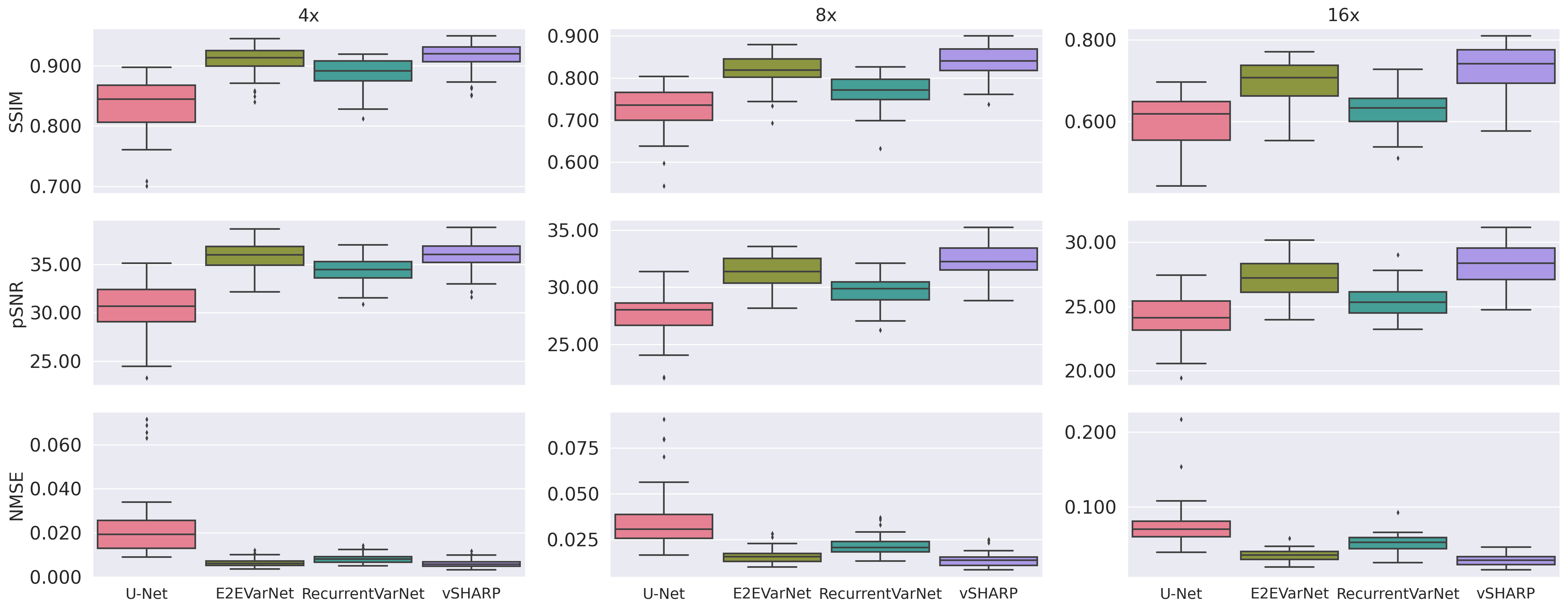
Figure 3: Box Plots illustrating the quantitative results on the fastMRI T2 prostate test set.

Table 2: Average evaluation metrics on the fastMRI T2 prostate test set.

Model	Metrics
	$4\times$			$8\times$			$16\times$
	SSIM	pSNR	NMSE	SSIM	pSNR	NMSE	SSIM	pSNR	NMSE
U-Net	0.8339 $\pm$ 0.0444	30.35 $\pm$ 2.60	0.0230 $\pm$ 0.0151	0.7264 $\pm$ 0.0536	27.48 $\pm$ 1.92	0.0361 $\pm$ 0.0163	0.6030 $\pm$ 0.0613	24.07 $\pm$ 1.80	0.0750 $\pm$ 0.0290
VarNet	0.9092 $\pm$ 0.0259	35.91 $\pm$ 1.69	0.0066 $\pm$ 0.0018	0.8171 $\pm$ 0.0386	31.37 $\pm$ 1.46	0.0162 $\pm$ 0.0042	0.6962 $\pm$ 0.0510	27.18 $\pm$ 1.41	0.0360 $\pm$ 0.0078
RecurrentVarNet	0.8861 $\pm$ 0.0256	34.36 $\pm$ 1.38	0.0084 $\pm$ 0.0020	0.7678 $\pm$ 0.0385	29.63 $\pm$ 1.25	0.0216 $\pm$ 0.0051	0.6271$\pm$ 0.0452	25.36 $\pm$ 1.30	0.0525 $\pm$ 0.0051
vSHARP	0.9150 $\pm$ 0.0255	36.00 $\pm$ 1.75	0.0061 $\pm$ 0.0018	0.8383 $\pm$ 0.0386	32.31 $\pm$ 1.64	0.0139 $\pm$ 0.0039	0.7295 $\pm$ 0.0557	28.26 $\pm$ 1.62	0.0299 $\pm$ 0.0076

Turning to Fig. 3 and Tab. 2, which showcase the quantitative results for the fastMRI prostate dataset, vSHARP once again emerges as a top performer. It consistently achieves the highest SSIM, pSNR, and lowest NMSE values across all acceleration factors.

Additional Comparisons

In Table 3, we present supplementary comparisons beyond the core performance metrics. In particular, we report inference time per volume in seconds (s) for the fastMRI prostate dataset and the total number of parameters in millions (M) for each of the considered MRI reconstruction methods.

Table 3: Average time (in seconds) to reconstruct a volume at inference (for the fastMRI prostate dataset) and total number of parameters (in millions) for each method.

Model	Average Inference Time per volume (s)	Number of Parameters (M)
U-Net	18	31
VarNet	22	373
RecurrentVarNet	32	7
vSHARP	37	93

Table 3 shows that vSHARP, while slightly slower in terms of inference time compared to some of the other methods, strikes a balance between computational efficiency and model size while maintaining a relatively moderate number of parameters (93 M). It’s important to note that the choice of the number of parameters for each method was carefully considered to ensure practical applicability during training. For instance, RecurrentVarNet’s inherently recurrent nature demands substantial GPU memory during training, limiting our capacity to use a higher number of parameters.

5.2 vSHARP Inference Ablation

As detailed in Section 3, our vSHARP model generates a sequence of reconstructions $\left\{\mathbf{x}^{t}\right\}_{t=1}^{T}$ during training, encompassing results from all optimization steps. These reconstructions, combined in a weighted average, contribute to the computation of the training loss function (Eq. 12). This motivates the idea of exploring the feasibility of using a reduced subset of optimization blocks for the reconstruction process.

Within this context, we revisited the inference phase using the vSHARP model, which was originally trained for our comparison experiments (as detailed in the preceding subsection). Instead of utilizing all trained optimization blocks (T=12), we opted to work with a select subset, specifically blocks 1, 2, 7, 10, 11, and 12, while removing the remaining trained blocks (3, 4, 5, 7, 8, 9). The rationale behind this selection lies in the fact that, as indicated by (12), the latter blocks contribute more weight to the loss computation and therefore, we retained blocks 10, 11, and 12. Blocks 1 and 2, being the first to interact with the zero-filled image, were also preserved. The inclusion of the $6^{\text{th}}$ block, positioned approximately in the middle of the optimization procedure, further diversified our selection.

This approach enabled us to evaluate the balance between computational efficiency and reconstruction quality of vSHARP, providing insights into the performance implications of employing a reduced number of optimization steps during the inference phase. In Fig. 4 and Tab. 4, we present the quantitative performance metrics for the reduced-vSHARP configuration applied to the fastMRI prostate dataset. Additionally, in Tab. 5, we provide the corresponding inference times. These results are compared with those obtained using the original vSHARP as well as the other methods used for comparison.

Despite the slightly lower reconstruction scores observed with the reduced configuration across all acceleration factors (4x, 8x, and 16x) compared to the full optimization process, it’s noteworthy that these results consistently outperformed those achieved by U-Net and RecurrentVarNet. Furthermore, the performance remained comparable with E2EVarNet, as detailed in in Fig. 4 and Tab. 4.

Nevertheless, as shown by Tab. 5, this configuration demonstrates a substantial reduction in the average inference time per volume, outperforming both the original vSHARP and state-of-the-art methods like RecurrentVarNet and E2EVarNet.

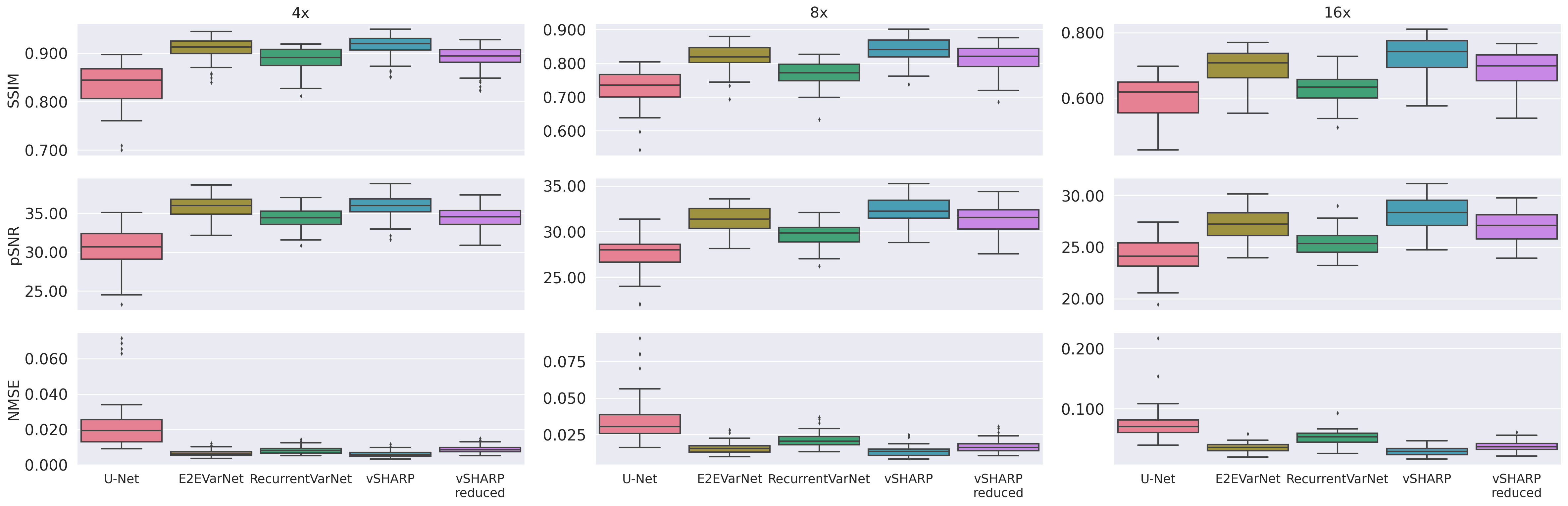
Figure 4: Box Plots illustrating the quantitative results on test set of fastMRI prostate dataset including vSHARP with reduced inference configuration using a subset of the $T$ optimization blocks (blocks 1, 2, 6, 10, 11, 12).

Table 4: Average Evaluation Metrics on Test Set of fastMRI prostate Dataset including vSHARP with reduced inference configuration using a subset of the $T$ optimization blocks (blocks 1, 2, 6, 10, 11, 12).

Model	Metrics
	$4\times$			$8\times$			$16\times$
	SSIM	pSNR	NMSE	SSIM	pSNR	NMSE	SSIM	pSNR	NMSE
U-Net	0.8339 $\pm$ 0.0444	30.35 $\pm$ 2.60	0.0230 $\pm$ 0.0151	0.7264 $\pm$ 0.0536	27.48 $\pm$ 1.92	0.0361 $\pm$ 0.0163	0.6030 $\pm$ 0.0613	24.07 $\pm$ 1.80	0.0750  pm 0.0290
VarNet	0.9092 $\pm$ 0.0259	35.91 $\pm$ 1.69	0.0066 $\pm$ 0.0018	0.8171 $\pm$ 0.0386	31.37 $\pm$ 1.46	0.0162 $\pm$ 0.0042	0.6962 $\pm$ 0.0510	27.18 $\pm$ 1.41	0.0360 $\pm$ 0.0078
RecurrentVarNet	0.8861 $\pm$ 0.0256	34.36 $\pm$ 1.38	0.0084 $\pm$ 0.0020	0.7678 $\pm$ 0.0385	29.63 $\pm$ 1.25	0.0216 $\pm$ 0.0051	0.6271$\pm$ 0.0452	25.36 $\pm$ 1.30	0.0525 $\pm$ 0.0051
vSHARP	0.9150 $\pm$ 0.0255	36.00 $\pm$ 1.75	0.0061 $\pm$ 0.0018	0.8383 $\pm$ 0.0386	32.31 $\pm$ 1.64	0.0139 $\pm$ 0.0039	0.7295 $\pm$ 0.0557	28.26 $\pm$ 1.62	0.0299 $\pm$ 0.0076
vSHARP-reduced	0.8896 $\pm$ 0.0270	34.36 $\pm$ 1.55	0.0089 $\pm$ 0.0023	0.8136 $\pm$ 0.0425	31.33 $\pm$ 1.67	0.0171 $\pm$ 0.0045	0.6881 $\pm$ 0.0535	27.02 $\pm$ 1.43	0.0380 $\pm$ 0.0086

Table 5: Average time (in seconds) to reconstruct a volume at inference (for the fastMRI prostate dataset) and total number of parameters for each method including vSHARP with reduced inference configuration using a subset of the $T$ optimization blocks (blocks 1, 2, 6, 10, 11, 12).

Model	Average Inference Time per volume (s)	Number of Parameters (m)
U-Net	18	31
VarNet	22	373
RecurrentVarNet	32	7
vSHARP	37	93
vSHARP-reduced	21	49

6 Conclusion and Discussion

In this work, we introduced vSHARP, a novel Deep Learning-based approach for solving ill-posed inverse problems in (Medical) Imaging. We proposed a versatile algorithm that combines the Half-Quadratic Variable Splitting method with the Alternating Direction Method of Multipliers, unrolling the optimization process and incorporating deep neural architectures for denoising and initialization. We applied vSHARP to the challenging task of accelerated parallel MRI reconstruction and conducted a comprehensive evaluation against state-of-the-art methods.

Our results in Section 5 demonstrate that vSHARP achieves superior performance in terms of quantitative evaluation metrics (SSIM, pSNR, NMSE) on two public $k$-space datasets, the Calgary Campinas brain and fastMRI prostate datasets. In our experiments, vSHARP consistently outperformed existing methods, showcasing its effectiveness in tackling the complex problem of accelerated MRI reconstruction, especially for high acceleration factors (8$\times$, 16$\times$).

One noteworthy observation stemming from our results is the fact that RecurrentVarNet, despite its competitive performance against vSHARP on the CC dataset, performed significantly poorer on the fastMRI prostate dataset. We attribute this discrepancy to its limited receptive field, which became a bottleneck when dealing with equispaced undersampling in the fastMRI prostate dataset, known for introducing substantial aliasing in the image domain. While increasing the number of parameters might enhance its performance, the recurrent nature of the network makes it challenging to fit in GPU memory during training. In contrast, both vSHARP and E2EVarNet, which employed U-Nets, benefited from a larger receptive field, enabling them to handle the aliasing caused by the equispaced undersampling more effectively.

Although in our experiments vSHARP exhibited superior performance against other state-of-the-art methods, it was bounded by longer reconstruction times when compared to the other methods. However, one notable aspect of vSHARP is its adaptability. In an ablation study in Section 5.2, we showed that it can be configured to use a reduced subset of optimization blocks during inference, which significantly reduces computational time while maintaining high reconstruction quality. This adaptability makes vSHARP a practical choice for applications where a trade-off between computation and reconstruction quality is needed. Note that we only experimented with using blocks 1, 2, 6, 10, 11, and 12 as a reduced set of optimization blocks, but alternative selections may yield even more promising results. The selection of these optimization blocks was primarily driven by their substantial contribution to the loss computation during training, sparking the idea of employing different weighting schemes, such as an equal weighting scheme across all optimization blocks.

Nevertheless, it is important to acknowledge some limitations and considerations. vSHARP assumes knowledge of the forward and adjoint operators, which might not always be straightforward to compute. For instance, in non-Cartesian accelerated MRI reconstruction, the computation of the non-uniform fast Fourier transform and its adjoint can be computationally expensive as it involves a gridding proccess. Additionally, while vSHARP demonstrated competitive performance in MRI reconstruction, its applicability to other ill-posed inverse problems in medical imaging, such as sparse-view CT or CBCT reconstruction, remains a subject of our future research.

In conclusion, vSHARP represents a promising advancement in the field of Medical Imaging. Its ability to combine the power of deep learning with mathematical optimization methods makes it a versatile and effective tool for solving ill-posed inverse problems.

Appendix A Additional Theory

A.1 ADMM Algorithm

ADMM in general, aims in solving problems possessing the following form:

$$\min_{\mathbf{x}\in\mathcal{X},\mathbf{z}\in\mathcal{Z}}f(\mathbf{x})+g(\mathbf{z}),\quad\text{subject to }{B}(\mathbf{x})+{C}(\mathbf{z})=d,\quad d\in\mathcal{D},$$ (20)

where $\mathcal{X}$, $\mathcal{Z}$, $\mathcal{D}$ are Hilbert spaces, and ${B}:\mathcal{X}\rightarrow\mathcal{D}$, ${C}:\mathcal{Z}\rightarrow\mathcal{D}$ are operators on $\mathcal{X}$ and $\mathcal{Z}$, respectively.

The Lagrangian for (20) is formulated as follows:

$$\mathcal{L}_{\rho}\left(\mathbf{x},\mathbf{z},\mathbf{u}\right)=f(\mathbf{x})+g(\mathbf{z})+\left<\mathbf{u},{B}(\mathbf{x})+{C}(\mathbf{z})-d\right>_{\mathcal{D}}+\frac{\rho}{2}\left|\left|{B}(\mathbf{x})+{C}(\mathbf{z})-d\right|\right|_{2}^{2},$$ (21)

where $\rho>0$, $\mathbf{u}$ are Lagrange multipliers, and $<\cdot,\cdot>_{\mathcal{D}}$ is an inner product on $\mathcal{D}$. ADMM then, consists of the following updated over $T$ iterations:

$$\mathbf{z}^{t+1}=\operatorname*{argmin}_{\mathbf{z}\in\mathcal{Z}}\mathcal{L}_{\rho}\left(\mathbf{x}^{t},\mathbf{z},\mathbf{u}^{t}\right)$$ (22a)

$$\mathbf{x}^{t+1}=\operatorname*{argmin}_{\mathbf{x}\in\mathcal{X}}\mathcal{L}_{\rho}\left(\mathbf{x},\mathbf{z}^{t+1},\mathbf{u}^{t}\right)$$ (22b)

$$\mathbf{u}^{t+1}=\mathbf{u}^{t}+\rho(\mathbf{x}^{t+1}-\mathbf{z}^{t+1}).$$ (22c)

A.2 ADMM for Inverse Problems

A solution to an inverse problem as defined in (1) can be formulated as a solution to (4). By using the notations for inverse problems defined in Section 2 and setting the following:

$$\mathcal{X}=\mathcal{Z}=\mathcal{D}$$ (23a)

$$f(\cdot):=\left|\left|\mathcal{A}(\cdot)-\tilde{\mathbf{y}}\right|\right|_{2}^{2}+\lambda\mathcal{R}(\cdot),\quad g:=0$$ (23b)

$${B}:=\boldsymbol{1}_{\mathcal{X}},\quad{C}:=-\boldsymbol{1}_{\mathcal{X}},\quad\mathbf{d}:=0,$$ (23c)

we can derive the ADMM updates for solving inverse problems as stated in (7c).

Appendix B Supplemental Material

B.1 Accelerated Parallel MRI Reconstruction

B.1.1 Image Domain Loss Functions Definitions

Absolute Differences Loss

$$\mathcal{L}_{1}(\mathbf{v},\mathbf{w})=||\mathbf{v}-\mathbf{w}||_{1}$$ (24)

Structural Similarity Index Measure Loss

$$\text{SSIMLoss}(\mathbf{v},\mathbf{w})=1-\text{SSIM}(\mathbf{v},\mathbf{w}),\quad\text{SSIM}(\mathbf{v},\,\mathbf{w})=\frac{1}{M}\sum_{i=1}^{M}\frac{(2\mu_{\mathbf{v}_{i}}\mu_{\mathbf{w}_{i}}+0.01)(2\sigma_{\mathbf{v}_{i}\mathbf{w}_{i}}+0.03)}{({\mu^{2}_{\mathbf{v}_{i}}}+{\mu^{2}_{\mathbf{w}_{i}}}+0.01)({\sigma^{2}_{\mathbf{v}_{i}}}+{\sigma^{2}_{\mathbf{w}_{i}}}+0.03)},$$ (25a)

$$\mu_{\mathbf{v}_{i}}=\text{Mean}(\mathbf{v}_{i}),\quad\mu_{\mathbf{w}_{i}}=\text{Mean}(\mathbf{w}_{i}),\quad\sigma^{2}_{\mathbf{v}_{i}}=\text{Var}(\mathbf{v}_{i}),\quad\sigma^{2}_{\mathbf{w}_{i}}=\text{Var}(\mathbf{w}_{i}),\quad\sigma_{\mathbf{v}_{i}\mathbf{w}_{i}}=\text{Cov}(\mathbf{v}_{i},\mathbf{w}_{i}),$$ (25b)

where $\mathbf{v}_{i},\,\mathbf{w}_{i},\,i=1,\cdots,M$ are $7\times 7$ image windows from $\mathbf{v}$ and $\mathbf{w}$, respectively.

High Frequency Error Norm Loss

$$\text{{HFEN}}_{1}(\mathbf{v},\,\mathbf{w})\,=\,\frac{||\text{{LoG}}(\mathbf{v})-\text{{LoG}}(\mathbf{w})||_{1}}{||\text{{LoG}}(\mathbf{v})||_{1}},\quad\text{{HFEN}}_{2}(\mathbf{v},\,\mathbf{w})\,=\,\frac{||\text{{LoG}}(\mathbf{v})-\text{{LoG}}(\mathbf{w})||_{2}}{||\text{{LoG}}(\mathbf{v})||_{2}},$$ (26)

where where LoG denotes a $15\times 15$ kernel filter of the Laplacian of a Gaussian distribution with standard deviation of 2.5.

B.1.2 k-space Domain Loss Functions

Normalized Mean Squared Error (NMSE)

$$\text{NMSE}(\mathbf{v},\,\mathbf{w})\,=\,\frac{||\mathbf{v}\,-\,\mathbf{w}||_{2}^{2}}{||\mathbf{v}||_{2}^{2}}$$ (27)

Normalized Mean Average Error (NMAE)

$$\text{NMAE}(\mathbf{v},\,\mathbf{w})\,=\,\frac{||\mathbf{v}\,-\,\mathbf{w}||_{1}}{||\mathbf{v}||_{1}}$$ (28)

B.1.3 Qualitative Results

In Figures A1 and A2, we present sample reconstructions obtained from our experiments conducted on the Calgary-Campinas and fastMRI prostate test sets. These reconstructions are accompanied by their corresponding undersampling patterns for all acceleration factors. Both Figures illustrate that vSHARP consistently delivers reconstructions with superior visual fidelity, underscoring its effectiveness in handling accelerated parallel MRI reconstruction, even for high acceleration factors such as 16$\times$.

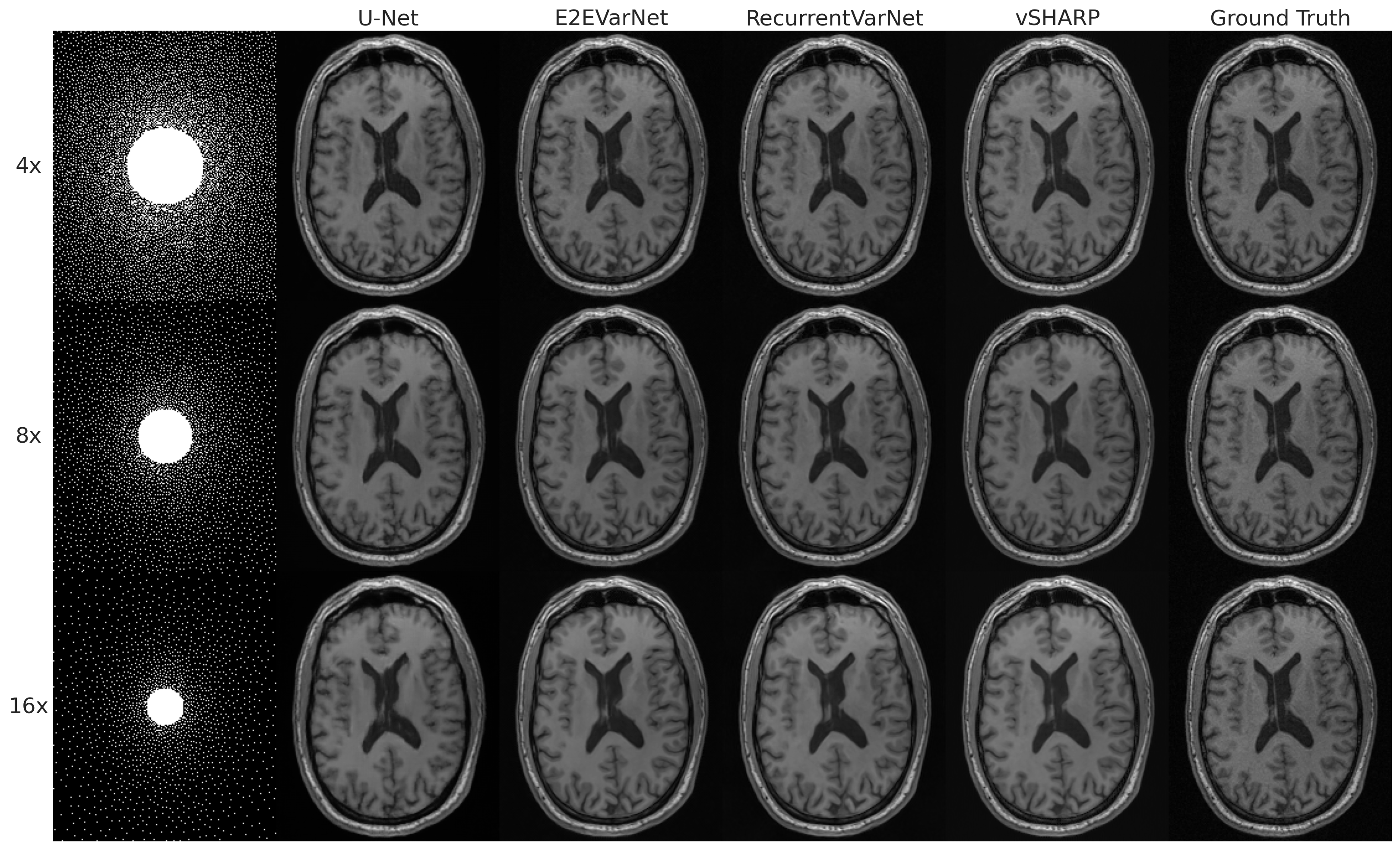
Figure A1 : Sample reconstructions from the Calgary-Campinas test set.

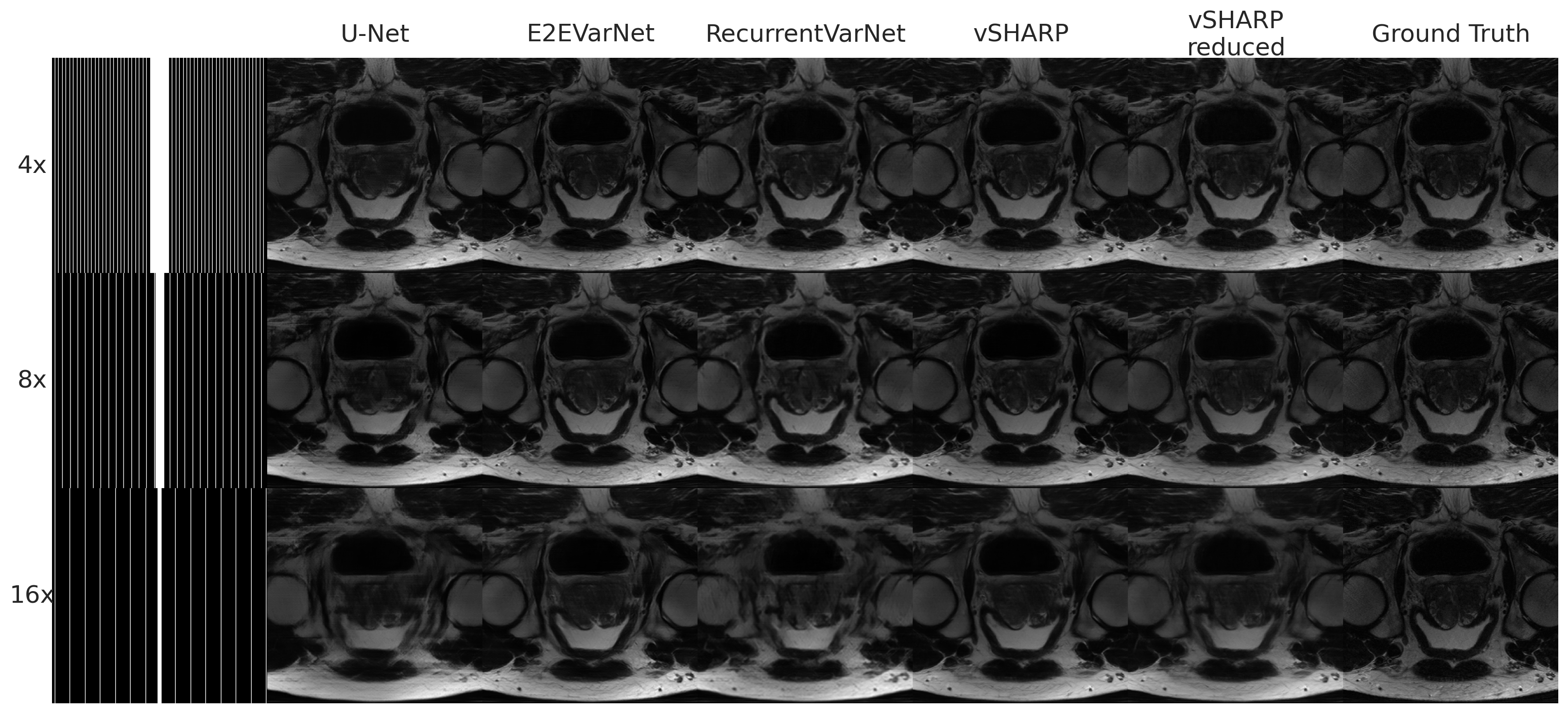
Figure A2 : Sample reconstructions from the fastMRI prostate test set.

References

- [1] James F. Glockner, Houchun H. Hu, David W. Stanley, Lisa Angelos, and Kevin King. Parallel MR imaging: A user’s guide. RadioGraphics, 25(5):1279–1297, September 2005.
- [2] Gregory Ongie, Ajil Jalal, Christopher A Metzler, Richard G Baraniuk, Alexandros G Dimakis, and Rebecca Willett. Deep learning techniques for inverse problems in imaging. IEEE Journal on Selected Areas in Information Theory, 1(1):39–56, 2020.
- [3] Maziar Raissi, Paris Perdikaris, and George E Karniadakis. Physics-informed neural networks: A deep learning framework for solving forward and inverse problems involving nonlinear partial differential equations. Journal of Computational physics, 378:686–707, 2019.
- [4] Alice Lucas, Michael Iliadis, Rafael Molina, and Aggelos K. Katsaggelos. Using deep neural networks for inverse problems in imaging: Beyond analytical methods. IEEE Signal Processing Magazine, 35(1):20–36, 2018.
- [5] Hemant K. Aggarwal, Merry P. Mani, and Mathews Jacob. Modl: Model-based deep learning architecture for inverse problems. IEEE Transactions on Medical Imaging, 38(2):394–405, 2019.
- [6] George Yiasemis, Jan-Jakob Sonke, Clarisa Sánchez, and Jonas Teuwen. Recurrent variational network: A deep learning inverse problem solver applied to the task of accelerated mri reconstruction. In Proceedings of the IEEE/CVF Conference on Computer Vision and Pattern Recognition (CVPR), pages 732–741, June 2022.
- [7] Anuroop Sriram, Jure Zbontar, Tullie Murrell, Aaron Defazio, C. Lawrence Zitnick, Nafissa Yakubova, Florian Knoll, and Patricia Johnson. End-to-end variational networks for accelerated mri reconstruction. In Anne L. Martel, Purang Abolmaesumi, Danail Stoyanov, Diana Mateus, Maria A. Zuluaga, S. Kevin Zhou, Daniel Racoceanu, and Leo Joskowicz, editors, Medical Image Computing and Computer Assisted Intervention – MICCAI 2020, Cham, 2020. Springer International Publishing.
- [8] Roberto Souza, Mariana Bento, Nikita Nogovitsyn, Kevin J. Chung, Wallace Loos, R. Marc Lebel, and Richard Frayne. Dual-domain cascade of u-nets for multi-channel magnetic resonance image reconstruction. Magnetic Resonance Imaging, 71:140–153, 2020.
- [9] Nikita Moriakov, Jan-Jakob Sonke, and Jonas Teuwen. Lire: Learned invertible reconstruction for cone beam ct. arXiv preprint arXiv:2205.07358, 2022.
- [10] Yang Zhang, Ning Yue, Min-Ying Su, Bo Liu, Yi Ding, Yongkang Zhou, Hao Wang, Yu Kuang, and Ke Nie. Improving cbct quality to ct level using deep learning with generative adversarial network. Medical physics, 48(6):2816–2826, 2021.
- [11] Frederic Madesta, Thilo Sentker, Tobias Gauer, and René Werner. Self-contained deep learning-based boosting of 4d cone-beam ct reconstruction. Medical Physics, 47(11):5619–5631, 2020.
- [12] Allard Adriaan Hendriksen, Daniel Maria Pelt, and K. Joost Batenburg. Noise2inverse: Self-supervised deep convolutional denoising for tomography. IEEE Transactions on Computational Imaging, 6:1320–1335, 2020.
- [13] Jaakko Lehtinen, Jacob Munkberg, Jon Hasselgren, Samuli Laine, Tero Karras, Miika Aittala, and Timo Aila. Noise2noise: Learning image restoration without clean data, 2018.
- [14] Kuanhong Cheng, Juan Du, Huixin Zhou, Dong Zhao, and Hanlin Qin. Image super-resolution based on half quadratic splitting. Infrared Physics & Technology, 105:103193, 2020.
- [15] Jian-Feng Cai and Ke Wei. Chapter 2 - exploiting the structure effectively and efficiently in low-rank matrix recovery. In Ron Kimmel and Xue-Cheng Tai, editors, Processing, Analyzing and Learning of Images, Shapes, and Forms: Part 1, volume 19 of Handbook of Numerical Analysis, pages 21–51. Elsevier, 2018.
- [16] Olaf Ronneberger, Philipp Fischer, and Thomas Brox. U-net: Convolutional networks for biomedical image segmentation, 2015.
- [17] Zhendong Wang, Xiaodong Cun, Jianmin Bao, Wengang Zhou, Jianzhuang Liu, and Houqiang Li. Uformer: A general u-shaped transformer for image restoration. In Proceedings of the IEEE/CVF Conference on Computer Vision and Pattern Recognition (CVPR), pages 17683–17693, June 2022.
- [18] Youssef Beauferris, Jonas Teuwen, Dimitrios Karkalousos, Nikita Moriakov, Matthan Caan, George Yiasemis, Lívia Rodrigues, Alexandre Lopes, Helio Pedrini, Letícia Rittner, Maik Dannecker, Viktor Studenyak, Fabian Gröger, Devendra Vyas, Shahrooz Faghih-Roohi, Amrit Kumar Jethi, Jaya Chandra Raju, Mohanasankar Sivaprakasam, Mike Lasby, Nikita Nogovitsyn, Wallace Loos, Richard Frayne, and Roberto Souza. Multi-coil MRI reconstruction challenge—assessing brain MRI reconstruction models and their generalizability to varying coil configurations. Frontiers in Neuroscience, 16, July 2022.
- [19] Radhika Tibrewala, Tarun Dutt, Angela Tong, Luke Ginocchio, Mahesh B Keerthivasan, Steven H Baete, Sumit Chopra, Yvonne W Lui, Daniel K Sodickson, Hersh Chandarana, and Patricia M Johnson. Fastmri prostate: A publicly available, biparametric mri dataset to advance machine learning for prostate cancer imaging, 2023.
- [20] David G Luenberger. Optimization by vector space methods. John Wiley & Sons, Nashville, TN, January 1997.
- [21] Sergey I. Kabanikhin. Inverse and Ill-posed Problems. DE GRUYTER, December 2011.
- [22] Amir Beck and Marc Teboulle. A fast iterative shrinkage-thresholding algorithm for linear inverse problems. SIAM Journal on Imaging Sciences, 2(1):183–202, 2009.
- [23] Wang Shuai, Xu Baiyan, and Liu Tao. A conjugate gradient method for inverse problems of non-linear coupled diffusion equations. Journal of Physics: Conference Series, 1634(1):012165, September 2020.
- [24] Stephen Boyd, Neal Parikh, Eric Chu, Borja Peleato, and Jonathan Eckstein. 2011.
- [25] Antonin Chambolle and Thomas Pock. A first-order primal-dual algorithm for convex problems with applications to imaging. Journal of Mathematical Imaging and Vision, 40(1):120–145, December 2010.
- [26] Manya V. Afonso, José M. Bioucas-Dias, and Mário A. T. Figueiredo. Fast image recovery using variable splitting and constrained optimization. IEEE Transactions on Image Processing, 19(9):2345–2356, 2010.
- [27] Kaiming He, Xiangyu Zhang, Shaoqing Ren, and Jian Sun. Deep residual learning for image recognition, 2015.
- [28] Songhyun Yu, Bumjun Park, and Jechang Jeong. Deep iterative down-up cnn for image denoising. In 2019 IEEE/CVF Conference on Computer Vision and Pattern Recognition Workshops (CVPRW), pages 2095–2103, 2019.
- [29] Guilin Liu, Aysegul Dundar, Kevin J. Shih, Ting-Chun Wang, Fitsum A. Reda, Karan Sapra, Zhiding Yu, Xiaodong Yang, Andrew Tao, and Bryan Catanzaro. Partial convolution for padding, inpainting, and image synthesis. IEEE Transactions on Pattern Analysis and Machine Intelligence, pages 1–15, 2022.
- [30] Fisher Yu and Vladlen Koltun. Multi-scale context aggregation by dilated convolutions. In International Conference on Learning Representations, 2016.
- [31] George Yiasemis, Clara I. Sánchez, Jan-Jakob Sonke, and Jonas Teuwen. On retrospective k-space subsampling schemes for deep mri reconstruction, 2023.
- [32] Erik G. Larsson, Deniz Erdogmus, Rui Yan, Jose C. Principe, and Jeffrey R. Fitzsimmons. SNR-optimality of sum-of-squares reconstruction for phased-array magnetic resonance imaging. Journal of Magnetic Resonance, 163(1):121–123, July 2003.
- [33] George Yiasemis, Nikita Moriakov, Dimitrios Karkalousos, Matthan Caan, and Jonas Teuwen. Direct: Deep image reconstruction toolkit, 2022.
- [34] Anuroop Sriram, Jure Zbontar, Tullie Murrell, Aaron Defazio, C. Lawrence Zitnick, Nafissa Yakubova, Florian Knoll, and Patricia Johnson. End-to-end variational networks for accelerated MRI reconstruction. In Medical Image Computing and Computer Assisted Intervention – MICCAI 2020, pages 64–73. Springer International Publishing, 2020.