TESS Spots a Super-Puff: The Remarkably Low Density of TOI-1420b

Abstract

We present the discovery of TOI-1420b, an exceptionally low-density ($\rho=0.08\pm 0.02$ g cm^-3) transiting planet in a $P=6.96$ day orbit around a late G dwarf star. Using transit observations from TESS, LCOGT, OPM, Whitin, Wendelstein, OAUV, Ca l’Ou, and KeplerCam along with radial velocity observations from HARPS-N and NEID, we find that the planet has a radius of $R_{\mathrm{p}}=11.9\pm 0.3R_{\earth}$ and a mass of $M_{\mathrm{p}}=25.1\pm 3.8M_{\earth}$. TOI-1420b is the largest-known planet with a mass less than $50M_{\earth}$, indicating that it contains a sizeable envelope of hydrogen and helium. We determine TOI-1420b’s envelope mass fraction to be $f_{\mathrm{env}}=82^{+7}_{-6}\%$, suggesting that runaway gas accretion occurred when its core was at most $4-5\times$ the mass of the Earth. TOI-1420b is similar to the planet WASP-107b in mass, radius, density, and orbital period, so a comparison of these two systems may help reveal the origins of close-in low-density planets. With an atmospheric scale height of 1950 km, a transmission spectroscopy metric of 580, and a predicted Rossiter-McLaughlin amplitude of about $17$ m s^-1, TOI-1420b is an excellent target for future atmospheric and dynamical characterization.

1 Introduction

Since the discovery of 51 Pegasi b nearly thirty years ago (Mayor & Queloz, 1995), over 5000 exoplanets have been detected to date. Many of these planets challenge our intuition from the Solar system. For instance, the Kepler mission (Borucki et al., 2010) revealed that sub-Neptunes and super-Earths (with $1R_{\earth}<R_{\mathrm{p}}<4R_{\earth}$ and $P<100$ days) occur around $30-60\%$ of Sun-like stars (e.g. Latham et al., 2011), despite not having a direct counterpart within the Solar System. The Solar System also exhibits a clear distinction between the ice giants ($M_{\mathrm{p}}\lesssim 20M_{\earth}$) and the gas giants ($M_{\mathrm{p}}\gtrsim 100M_{\earth}$). Many planets have now been detected with masses between that of Neptune and Saturn, although they are less common than sub-Neptunes and more challenging to detect than gas giants (Petigura et al., 2018).

Table 1: Summary of Stellar Parameters for TOI-1420

Parameters	Description (Units)	Values	Source
Main Identifiers:
TOI	…	1420	TESS Mission
TIC	…	321857016	TIC
Tycho-2	…	4261-149-1	Tycho-2
2MASS	…	J21314590+6620556	2MASS
AllWISE	…	J213145.99+662056.2	AllWISE
Gaia DR3	…	2221164434736927360	Gaia DR3
Coordinates & Proper Motion:
$\alpha_{J2000}$	Right Ascension (RA)	21:31:45.917	Gaia DR3
$\delta_{J2000}$	Declination (Dec)	+66:20:55.925	Gaia DR3
$\mu_{\alpha}$	RA Proper Motion (mas/yr)	45.482 ± 0.013	Gaia DR3
$\mu_{\delta}$	Dec Proper Motion (Dec, mas/yr)	31.874 ± 0.012	Gaia DR3
$\varpi$	Parallax (mas)	4.9134 ± 0.0105	Gaia DR3
$d$	Distance (pc)	201.84 ± 0.43	Gaia DR3
Magnitudes:
$G$	Gaia $G$ Magnitude	11.7323 ± 0.0002	Gaia DR3
$B_{P}$	Gaia $B_{P}$ Magnitude	12.1338 ± 0.0007	Gaia DR3
$R_{P}$	Gaia $R_{P}$ Magnitude	11.1707 ± 0.0006	Gaia DR3
$T$	TESS Magnitude	11.229 ± 0.006	TIC
$J$	2MASS $J$ Magnitude	10.557 ± 0.022	2MASS
$H$	2MASS $H$ Magnitude	10.191 ± 0.021	2MASS
$K_{s}$	2MASS $K_{s}$ Magnitude	10.119 ± 0.022	2MASS
$W1$	WISE $W1$ Magnitude	10.059 ± 0.023	AllWISE
$W2$	WISE $W2$ Magnitude	10.120 ± 0.021	AllWISE
$W3$	WISE $W3$ Magnitude	10.084 ± 0.044	AllWISE
Spectroscopic Parameters:
$[$Fe/H]	Metallicity (dex)	0.29 ± 0.08	This work (HARPS-N)
$T_{\mathrm{eff}}$	Effective Temperature (K)	5493 ± 50	This work (HARPS-N)
$\log(g)$	Surface gravity (cgs)	4.49 ± 0.10	This work (HARPS-N)
$v\sin i_{\star}$	Rotational velocity (km s-1)	<2	This work (HARPS-N)

Note. — References are: TIC (Stassun et al., 2018), Tycho-2 (Høg et al., 2000), 2MASS (Cutri et al., 2003), AllWISE (Cutri et al., 2021), Gaia DR3 (Gaia Collaboration et al., 2022). Gaia DR3 RA and Dec have been corrected from epoch J2016 to J2000. $v\sin i_{\star}$ has not been corrected for macroturbulence, and is therefore larger than the true $v\sin i_{\star}$. Floor errors have been adopted on $[\mathrm{Fe/H]}$, $T_{\mathrm{eff}}$, and $\log(g)$ to account for residual systematic errors.

One important feature of this intermediate-mass population is its compositional diversity, which (at least in a bulk sense) can be inferred when both masses and radii are well-measured (Lopez & Fortney, 2014; Thorngren et al., 2016). Transiting planets with $20M_{\earth}<M_{\mathrm{p}}<100M_{\earth}$ span a wide range of sizes, indicating a wide range of compositions for the population (Petigura et al., 2017). Their compositions are broadly consistent with expectations from formation models except for a striking population of low-mass low-density outliers, sometimes called “super-puffs” (Lee & Chiang, 2016; Lee, 2019). These mysteriously low-density ($\rho\lesssim 0.2$ g cm^-3) planets were unanticipated by formation models, as they appear to have accreted voluminous H/He envelopes despite having smaller cores than typically required for runaway gas accretion.

Such low-density outcomes of planet formation are still not fully understood, in part because they are rare. There are only 15 planets in this intermediate mass regime ($20M_{\earth}<M_{\mathrm{p}}<100M_{\earth}$) with densities below $\rho\leq 0.2$ g cm^-3 (per the NASA Exoplanet Archive on 23 March 2023; Akeson et al., 2013), and many reside in systems too faint for precise characterization. Detecting new low-density worlds in bright systems will help enable comparative planetology in this puzzling population. The Transiting Exoplanet Survey Satellite (TESS; Ricker et al., 2015) is playing an important role in detecting new puffy planets in systems amenable to follow-up efforts (e.g. McKee & Montet, 2022).

To this end, we report the discovery of an exceptionally low-density ($\rho=0.08\pm 0.02$ g cm^-3) planet orbiting the late G dwarf star TOI-1420 every 6.96 days. The planet TOI-1420b has a size similar to that of Jupiter ($R_{\mathrm{p}}=11.9\pm 0.3R_{\earth}$) but a mass similar to that of Neptune ($M_{\mathrm{p}}=25.1\pm 3.8M_{\earth}$). In Section 2 we describe the TESS observations that revealed the initial transit signals, as well as the follow-up photometric, spectroscopic, and imaging observations that ultimately confirmed the planet. In Section 3, we present a global fit to the aforementioned observations using EXOFASTv2. We then examine the structure of this intriguingly low-density planet in Section 4, and finally we conclude with a look towards future observations in Section 5.

2 Observations

2.1 TESS Photometry

TOI-1420 (stellar parameters provided in Table 1) was selected for 2-minute cadence observations with the TESS mission starting in Sector 16. Raw photometric data were processed by the TESS Science Processing Operations Center (SPOC; Jenkins et al., 2016), based at the NASA Ames Research Center, and the resulting light curves were available to download from the Mikulski Archive for Space Telescopes (MAST). The SPOC conducted a transit search of Sector 16 on 2019 October 22 with an adaptive, noise-compensating matched filter (Jenkins, 2002; Jenkins et al., 2010), producing a threshold-crossing event (TCE) for which an initial limb-darkened transit model was fitted (Li et al., 2019) and a suite of diagnostic tests were conducted to help make or break the planetary nature of the signal (Twicken et al., 2018). The TESS Science Office (TSO) reviewed the vetting information and issued an alert on 2019 November 6 (Guerrero et al., 2021). The signal was repeatedly recovered as additional observations were made in sectors 24, 56, 57 and 58. The transit signature passed all the diagnostic tests presented in the Data Validation reports. According to the difference image centroiding tests, the host star is located within $0\farcs 339\pm 2\farcs 61$ of the transit signal source.

In our analysis, we included the 2 minute cadence data from Sectors 16, 24, 56, 57, and 58 (Figure 1). Data from Sectors 17 and 18 were taken only at 30 minute cadence and were not included. For the five 2 minute cadence Sectors, we obtained the Presearch Data Conditioning Simple Aperture Photometry (PDCSAP) light curves (Smith et al., 2012; Stumpe et al., 2012, 2014) using the lightkurve package (Lightkurve Collaboration et al., 2018). We used lightkurve to detrend the light curves with a Savitsky-Golay filter, applying a window length of 66.7 hours (with the transit events masked, each with a duration of 3.37 hours), and we subsequently removed any $\geq 5\sigma$ outliers from the light curves.

While detrending the TESS light curves, we noticed that some of the sectors exhibit periodic photometric variability on a 7 day timescale (close to the planetary orbital period); this was confirmed via a Lomb-Scargle periodogram and autocorrelation analysis. Moreover, in these cases the planetary transits seem to be phased up with the $\sim$500 ppm photometric variability. We show in Figure 2 that the periodic variability appears fairly persistent across most TESS sectors, although the signal is not detected in Sector 57 and is fairly weak in Sector 58. Given this, it was especially important to use ground-based follow-up observations to test whether an on-target eclipsing binary (EB) or nearby eclipsing binaries (NEBs) blended with the target star within the TESS aperture were responsible for the observed transit signals in TESS. We note that the system is currently included in the TESS Eclipsing Binary catalog albeit with an “ambiguous” disposition (Prša et al., 2022).

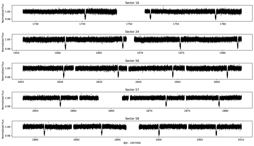
Figure 1: TESS 2 min cadence PDCSAP light curves for TOI-1420. Transit events are visible roughly every 7 days.

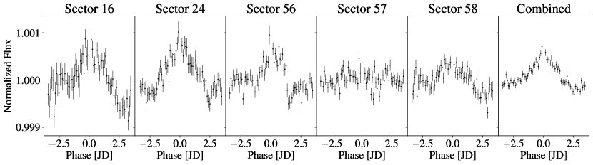
Figure 2: TESS PDCSAP light curves for TOI-1420 phased to the planetary ephemeris and binned to 0.1 day cadence. The transits are masked and occur at a phase of 0 days.

2.2 Ground-based Photometry

Table 2: Summary of Ground-Based Light Curve Observations

Date	Observatory	Filter	Coverage	Size	Pixel Scale
(UT)				(m)	($\arcsec$)
2019-11-27	LCOGT	$I$	Ingress	2.0	0.30
2020-02-04	OPM	$B$	Full	0.2	0.69
2020-11-08	Whitin	$z^{\prime}$	Full	0.7	0.67
2021-01-03	Wendelstein	$i$	Full	0.4	0.64
2021-05-15	OAUV	$B$	Egress	0.5	0.54
2021-11-06	Ca l’Ou	$B$	Full	0.4	1.11
2022-06-23	KeplerCam	$i^{\prime}$	Ingress	1.2	0.67
2022-08-11	LCOGT	$B$	Full	1.0	0.39
2022-08-11	LCOGT	$g^{\prime}$	Full	1.0	0.39
2022-08-11	LCOGT	$i^{\prime}$	Full	1.0	0.39
2022-08-11	LCOGT	$z_{s}$	Full	1.0	0.39

The TESS pixel scale is $\sim 21\arcsec$ pixel^-1 and photometric apertures typically extend out to roughly 1 arcminute, generally causing multiple stars to blend in the TESS aperture. To rule out an NEB blend as the potential source of the TOI-1420.01 TESS detection and attempt to detect the signal on-target, we observed the field as part of the TESS Follow-up Observing Program Sub Group 1 (TFOP; Collins, 2019). We observed in multiple bands across the optical spectrum to check for wavelength dependent transit depth, which can also be suggestive of a planet candidate false positive. We used the TESS Transit Finder, which is a customized version of the Tapir software package (Jensen, 2013), to schedule our transit observations. All light curve data are available on the EXOFOP-TESS website.

In total, we obtained 11 follow-up observations from seven unique observatories: Observatoire Privé du Mont (OPM), Whitin Observatory, Wendelstein Observatory, Observatori Astronòmic de la Universitat de València (OAUV), Observatori de Ca l’Ou, KeplerCam, and the Las Cumbres Observatory Global Telescope (LCOGT; Brown et al., 2013) 1 m and 2 m networks. Parameters for these follow-up observations are provided in Table 2. All data were both calibrated and processed using AstroImageJ (Collins et al., 2017) except for the LCOGT light curves, which were initially calibrated using the standard LCOGT BANZAI pipeline (McCully et al., 2018a, b).

The transit light curves are shown in Figure 3. In all cases, transit events were detected on-target, and on-time relative to the ephemerides from TESS. The depth of the detected events matched the depth in the TESS light curves, and the transits were achromatic (as determined by independent fits to the light curves, where the transit depths were all consistent with that observed by TESS). Thus, NEB blends were confidently ruled out as the source of the transit signal.

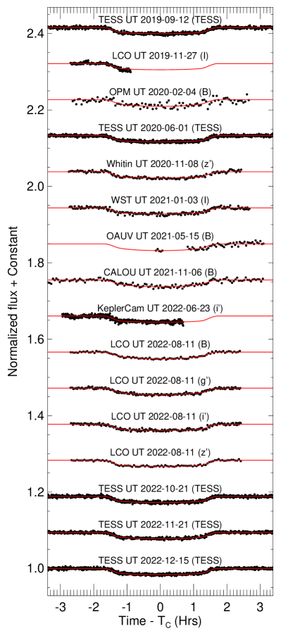
Figure 3: Transit light curves of TOI-1420b with TESS and ground-based observatories. Red curves indicate the best-fit EXOFASTv2 model.

2.3 Radial Velocity Observations

To measure the mass of TOI-1420.01 and/or rule out an on-target EB as the source of the transit events, we scheduled reconnaissance spectroscopy observations with the Tillinghast Reflector Echelle Spectrograph (TRES). TRES is a fiber-fed optical echelle spectrograph on the 1.5-meter Tillinghast telescope at the Fred Lawrence Whipple Observatory on Mt. Hopkins in Arizona with a resolving power of 44,000 (Szentgyorgyi & Furész, 2007). Eight measurements were taken between 2019 December 6 and 2021 June 27 with exposure times ranging from 1200 s to 2700 s. Though the planet was not massive enough to be detected by TRES with radial velocities (RVs), the non-detection ruled out the possibility of an EB.

The TRES observations indicated the spectrum of TOI-1420b was well suited for precise radial-velocity observations using the High Accuracy Radial velocity Planet Searcher for the Northern hemisphere (HARPS-N) at the 3.6m Telescopio Nazionale Galileo (TNG) in La Palma, Spain (Cosentino et al., 2012, 2014). HARPS-N is a highly stabilized echelle spectrograph with a resolving power of $R\sim 115,000$ capable of measuring radial velocities in the m s^-1 regime. We observed TOI-1420 between 2021 October 25 and 2022 September 5 (Table 3) and amassed a total of 44 observations using 1800 s exposures. We extracted RVs from these observations using v2.3.5 of the HARPS-N Data Reduction Software, which cross-correlates each observed spectrum with a weighted binary mask to estimate the RV (Pepe et al., 2002; Dumusque, 2018). Five observations were removed either due to their low SNRs ($<20$) or due to the Rossiter-McLaughlin effect during transits (Ohta et al., 2005). The final data set had internal precisions ranging from 1.9 to 5.4 m s^-1, in line with the anticipated precisions. A Lomb-Scargle periodogram of the HARPS-N RVs alone revealed a signal at 6.9 days, consistent with the orbital period obtained from the TESS light curve. We also verified that the phasing of the RVs was independently consistent with the reported transit ephemeris. We used the HARPS-N spectra to constrain the stellar effective temperature $T_{\mathrm{eff}}$, surface gravity $\log(g)$, metallicity [Fe/H], and projected rotational velocity $v\sin i$ using the Stellar Parameter Classification code (SPC; Buchhave et al., 2012; Bieryla et al., 2021). These measurements are reported in Table 1 along with other stellar parameters from the literature.

We also obtained 14 RV measurements with the NN-explore Exoplanet Investigations with Doppler spectroscopy (NEID) instrument, a high-resolution ($R\sim 110,000$) spectrograph at the WIYN 3.5-meter telescope on Kitt Peak, Arizona (Halverson et al., 2016; Schwab et al., 2016; Stefansson et al., 2016; Kanodia et al., 2018; Robertson et al., 2019). We obtained 990 s exposures with the high resolution fiber between 2022 April 2 and 2022 June 6. The standard NEID data reduction pipeline was used to obtain RVs from these observations, which are included in Table 3. RV precisions ranged from 2.5 to 7.5 m s^-1, in line with the anticipated precision of 3.2 m s^-1 from the NEID Exposure Time Calculator and sufficient to detect the planetary signal at $>3\sigma$ confidence in the NEID data. We also re-derived the RVs using the SERVAL pipeline optimized for NEID (Zechmeister et al., 2018; Stefànsson et al., 2022), and confirmed that the RV signal observed with NEID was robust to different data processing schemes.

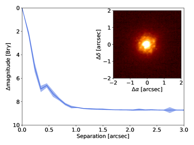
Figure 4: Sensitivities of our SAI-2.5 m $I_{c}$-band speckle image (left) and Gemini/NIRI Br$\gamma$ AO image (right). The insets are the high-resolution images of TOI-1420. The star appears single, and no visual companions are observed anywhere in either field of view, which extend to $5\farcs 1\times 10\farcs 6$ for the SAI image and $26\arcsec\times 26\arcsec$ for the Gemini/NIRI image (we only show the central few $\arcsec$ in the contrast curves and inset images for visual clarity).

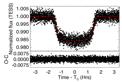
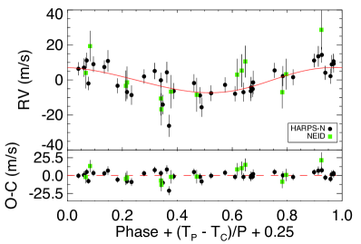
Figure 5: Left: Phase-folded light curve of TESS transits (left) and phase-folded HARPS-N and NEID RVs of TOI-1420 (right) with residuals. The black data points are the observations and the red lines are the overlaying best-fit models from ExoFASTv2.

Table 3: TOI-1420 RV Measurements from HARPS-N and NEID

BJDTDB	RV (m s-1)	$\sigma_{\mathrm{RV}}$ (m s-1)
HARPS-N Measurements:
2459513.43049	-10332.6	3.2
2459514.45289	-10325.9	3.1
2459515.39936	-10325.3	2.8
…	…	…
2459826.46509	-10328.9	5.8
2459828.50094	-10316.8	2.8
NEID Measurements:
2459736.87178	-10253.7	2.8
2459733.95347	-10263.7	4.6
2459732.84176	-10258.4	3.5
…	…	…
2459679.98135	-10254.0	3.6
2459672.00255	-10265.5	4.9

Note. — Table 3 is published in its entirety in machine-readable format. A portion is shown here for guidance regarding its form and content.

2.4 High-Resolution Imaging

It is important to vet for close visual companions that can dilute the lightcurve and thus alter the measured radius, or cause false positives if the companion is itself an eclipsing binary (e.g. Ciardi et al., 2015). To search for nearby companions that are unresolved in TESS or in ground-based seeing-limited images, we obtained high-resolution images of TOI-1420.

We observed TOI-1420 on 2020 December 2 UT with the Speckle Polarimeter (Safonov et al., 2017) on the 2.5 m telescope at the Caucasian Observatory of Sternberg Astronomical Institute (SAI) of Lomonosov Moscow State University. The speckle polarimeter uses an Electron Multiplying CCD Andor iXon 897 as a detector. The atmospheric dispersion compensator allowed observation of this relatively faint target through the wide-band $I_{c}$ filter. The power spectrum was estimated from 4000 frames with 30 ms exposure. The detector has a pixel scale of $20.6$ mas pixel^-1, and the angular resolution was 89 mas. We did not detect any stellar companions brighter than $\Delta I_{C}=4.5$ and $6.6$ at $\rho=0\farcs 25$ and $1\farcs 0$, respectively, where $\rho$ is the separation between the source and the potential companion. The speckle image of the target is shown in Figure 4 along with the 5$\sigma$ contrast curve.

We also vetted for close companions with adaptive optics (AO) imaging using Gemini/NIRI (Hodapp et al., 2003). We collected 9 science images on 2019 November 13, each with exposure time 18 s, using the Br$\gamma$ filter. The telescope was dithered between exposures in a grid pattern. We used the dither frames themselves to reconstruct a sky background, which was subtracted from all frames. We also corrected for bad pixels, flat-fielded, and then aligned frames based on the stellar position and co-added the stack of images. We finally determined the sensitivity of these observations as a function of radius by injecting fake companions, and scaling their brightness such that they are detected at 5$\sigma$. This was repeated at several radii and position angles, and sensitivities were averaged azimuthally. We do not detect companions anywhere within the field of view ($26\arcsec\times 26\arcsec$ centered on TOI-1420). The data are sensitive to companions 5 magnitudes fainter than the star (=1% flux dilution) beyond 232 mas from TOI-1420, and to companions 8.7 magnitudes fainter than the star in the background-limited regime. In Figure 4 we show the AO image of the target, as well as the sensitivity as a function of radius of these observations.

2.5 Summary of Follow-Up Observations

With our follow-up data, we can confidently rule out false positive scenarios for TOI-1420.01. The seeing-limited photometry from Section 2.2 localizes the transit signal to TOI-1420, which is not in a visual binary, and thus NEB blend scenarios are ruled out. The high-resolution imaging from Section 2.4 rules out a closer AO binary with multiple independent observations. Taken together with the low Gaia DR3 Renormalized Unit Weight Error (RUWE) of 0.866 (indicative of an acceptable single-star astrometric fit), these data indicate that TOI-1420 is indeed a single star. If the system were an EB, our RVs in Section 2.3 would have easily detected a stellar-mass object in a 7 day orbit around TOI-1420. Instead, they show that the object is only $25.1\pm 3.8M_{\earth}$, as described in the following section. Thus we conclude that that object in orbit is unambiguously a planet. We hereafter refer to the planet as TOI-1420b and proceed to fit for the planetary parameters.

While we have ruled out EB false positive scenarios, the nature of the variability signal in the PDCSAP light curves shown in Figure 2 remains somewhat unclear. We searched for similar variability in the PDCSAP light curves of nearby stars, but did not detect it, suggesting that the signal may not be instrumental in origin. The variability is not detected in ASAS-SN photometry of TOI-1420 (Shappee et al., 2014; Kochanek et al., 2017), but the photometric errors are too large (1-2%) to be definitive. Next, we addressed the possibility that the variability was tracing stellar rotation. In Figure 6, we show periodograms for a number of spectroscopic activity tracers from HARPS-N alongside a periodogram of the HARPS-N RVs. None of the activity tracers exhibit variations on a 7 d timescale, suggesting that this is not the true stellar rotation period.

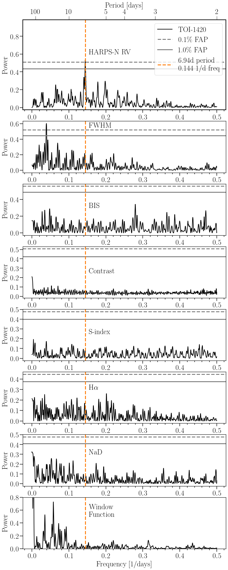
Figure 6: Periodograms of TOI-1420’s HARPS-N radial velocities, activity indicators, and window function. The False Alarm Probabilities (FAPs) are calculated via 100,000 bootstrap simulations. The only significant peak (<0.1% FAP) in the RV periodogram is at 6.94 days, which we attribute to the planet candidate. This periodic signal is not present in any of the activity indicators.

To test whether this signal could be attributed to an uncorrected TESS systematic in the PDCSAP reduction, we used the Systematics-Insensitive Periodogram (SIP; Hedges et al., 2020), which fits a linear noise model to the SAP light curves (with the transits masked) alongside a periodogram. We found that the SIP was unable to recover the 7 day periodicity, suggesting that the noise model was able to remove the variability signal. We conclude that the variability in Figure 2 may be a TESS systematic that was left uncorrected by the PDCSAP pipeline. The orbital period of the TESS spacecraft is close to 14 days, nearly twice the orbital period of the planet, which may explain why the signal appeared to be correlated with the planetary orbit. In any case, the detrending procedure we applied in Section 2.1 removed the out-of-transit variations, minimizing any impact on our final inferred radius in the global fit.

Table 4: TOI-1420 Stellar and Planetary Properties

Parameters	Description (Units)	Posterior Values
Stellar Parameters:
$M_{*}$	Stellar Mass ($M_{\odot}$)	0.987 ± 0.048
$R_{*}$	Stellar Radius ($R_{\odot}$)	0.923 ± 0.024
$L_{*}$	Stellar Luminosity ($L_{\odot}$)	0.705 ± 0.059
$\rho_{*}$	Stellar Density (g cm-3)	1.77 ± 0.16
$\log(g)$	Stellar surface gravity (cgs)	4.502 ± 0.029
$[$Fe/H]	Metallicity (dex)	0.280 ± 0.074
$\varpi$	Parallax (mas)	4.951 ± 0.030
$T_{\mathrm{eff}}$	Effective Temperature (K)	5510 ± 110
Age	Age (Gyr)	$<10.7$
$d$	Distance (pc)	202 ± 1.2
$A_{v}$	$V$-band Extinction (mag)	0.22 ± 0.11
Planetary Parameters:
$P$	Orbital Period (days)	6.9561063 ± 0.0000017
$T_{0}$	Transit Epoch (BJDTDB)	2459517.43305 ± 0.00012
$R_{p}$	Planetary Radius ($R_{\earth}$)	11.89 ± 0.33
$M_{p}$	Planetary Mass ($M_{\earth}$)	25.1 ± 3.8
$\rho_{p}$	Density (g cm-3)	0.082 ± 0.015
$R_{p}/R_{\star}$	Planet-to-star radius ratio	0.11816 ± 0.00059
$a/R_{\star}$	Semi-major axis/Stellar radius	16.53 ± 0.47
$\delta$	Transit Depth (%)	1.396 ± 0.014
$i$	Orbital Inclination (∘)	88.58 ± 0.13
$a$	Semi-major axis (au)	0.0710 ± 0.0012
$e$	Eccentricity	$<0.17$
$\omega_{\star}$	Argument of periastron (∘)	-165 ± 77
$K$	RV Semi-amplitude (m s-1)	8.5 ± 1.3
$T_{14}$	Transit duration (days)	0.1405 ± 0.0061
$b$	Impact Parameter	0.412 ± 0.036
$F$	Incident Flux (Gerg s-1 cm-2)	0.189 ± 0.014
$T_{\mathrm{eq}}$	Equilibrium Temperature (K)	957 ± 17

Note. — Priors are as described in EXOFASTv2 described in Eastman et al. (2019) with the addition of a metallicity prior from HARPS-N (Table 1) and a parallax prior from Gaia DR3 (Table 1) corrected for the bias reported by Lindegren et al. (2021). We did not impose additional priors on the spectroscopic parameters $T_{\mathrm{eff}}$ and $\log(g)$, as these can suffer from systematic errors (e.g. Eastman et al., 2019), so we fit them in ExoFAST independently to ensure we are not biased by systematic errors in the spectroscopy. Equilibrium temperature assumes zero albedo as described in Eastman et al. (2019). Upper limits are at 2$\sigma$.

3 Global Fit

We used the software package EXOFASTv2 (Eastman et al., 2019) to derive the stellar and planetary masses and radii from a joint solution of all the available photometry and spectroscopy. We used the TESS 2-minute cadence light curves, all ground based light curve observations, and the HARPS-N and NEID RV measurements. For the RV datasets, we fit for separate zero-point offsets and jitter values. We fit for the planetary radius, planetary mass, orbital inclination, orbital eccentricity, argument of periastron, orbital period, transit epoch, stellar temperature, stellar mass, stellar radius, stellar metallicity, stellar limb darkening coefficients visual extinction, distance, and parallax. The Markov Chain Monte Carlo (MCMC) fit was run with parallel tempering using 8 temperatures and 152 chains. We saved 7200 steps after thinning by a factor of 40. A burn-in period removed as described in Section 23.2 of Eastman et al. (2019). We ensured that the Gelman-Rubin statistics for all parameters were $<$ 1.01 to indicate that the fit had sufficiently full convergence (Gelman & Rubin, 1992).

The results of this global fit are presented in Table 4. Posteriors on additional fitting parameters including quadratic limb darkening coefficients, RV offsets and jitters, and added photometric variances are provided in the Appendix. We show the best-fit model with all ground and space-based light curves in Figure 3. The phased TESS photometry, HARPS-N RVs, and NEID RVs are shown in Figure 5 along with our best-fit solution. We find that the planet has a remarkably low density of just $0.082\pm 0.015$ g cm^-3. We verified the results of this global analysis by fitting the TESS photometry, HARPS-N RVs, and NEID RVs using the exoplanet package (Foreman-Mackey et al., 2021). We used broad uniform priors on all parameters except for the stellar mass and radius, where we used the distributions from Table 4. The posterior probability distributions from the exoplanet fit agreed with those from the EXOFASTv2 fit to better than 1$\sigma$.

4 Discussion

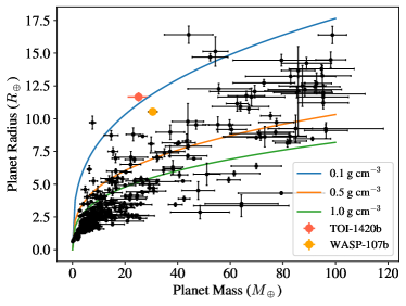
Figure 7: Mass-radius diagram of transiting planets from the NASA Exoplanet Archive with $0_{\earth}<M_{\mathrm{p}}<100M_{\earth}$ and better than 30% precision on the mass. The blue, orange, and green curves indicate 0.1 g cm^-3, 0.5 g cm^-3, and 1.0 g cm^-3, respectively. TOI-1420 (red point) is extremely low density and falls along the 0.1 g cm^-3 line.

In Figure 7, we present this new discovery in context on a mass-radius diagram of all known sub-Saturn mass planets (i.e. $20M_{\earth}<M_{p}<100M_{\earth}$) from the NASA Exoplanet Archive. The nearest neighbor to TOI-1420b on this plot is WASP-107b (Anderson et al., 2017), an important target for studies of planetary atmospheres, dynamics, structure, and formation (Kreidberg et al., 2018; Spake et al., 2018; Piaulet et al., 2021; Rubenzahl et al., 2021). TOI-1420b is larger and lower-mass than WASP-107b. Our newly-discovered planet also has a similar density to KELT-11b (Pepper et al., 2017), WASP-127b (Lam et al., 2017), and WASP-193b (Barkaoui et al., 2023), three puffy ($\rho\lesssim 0.1$ g cm^-3) planets with around twice the total mass of TOI-1420b. However, these three planets have equilibrium temperatures $T_{\mathrm{eq}}>1000$ K and are thus likely to be inflated by the hot Jupiter radius inflation mechanism (e.g. Fortney et al., 2021), whereas WASP-107b and TOI-1420b are too cool for substantial radius inflation.

Of these nearest neighbors, WASP-107b is particularly notable because it has an extreme envelope mass fraction of $>85\%$, corresponding to a low core mass of $<4.6M_{\earth}$ (Piaulet et al., 2021). Given that TOI-1420b appears to be even more anomalous than WASP-107b, we constrained its bulk metallicity using a planetary structure model. We use the cool giant planet interior structure models of (Thorngren et al., 2016) updated to use the Chabrier et al. (2019) equations of state for H and He. Matching these models to the observed parameters was done using the Bayesian framework described in Thorngren & Fortney (2019).

In Figure 8, we show the posterior probability distribution for the bulk metallicity, where we find $Z_{p}=0.18^{+0.07}_{-0.06}$. This corresponds to an envelope mass fraction $f_{\mathrm{env}}=1-Z_{p}=0.82^{+0.07}_{-0.06}$ and an inferred core mass of at most $M_{\mathrm{core}}=M_{p}Z_{p}<4.3^{+2.0}_{-1.7}M_{\earth}$, similar to that of WASP-107b. The inferred core mass is an upper limit because the atmosphere may contain some metals (decreasing the amount available in the assumed core). There is a covariance with the age of the system (which is not well-constrained by our data): even with a larger metal fraction, a young planet would be puffy and match the observed radius. These calculations were run with no anomalous heating included, but because the planet is close to the hot Jupiter heating threshold of $F=2\times 10^{8}$ erg s^-1 cm^-2 (see e.g. Miller & Fortney, 2011), we re-ran the structure models with the radius decreased by 5% to account for the possible weak heating. In this case we found $Z_{p}=0.20\pm 0.06$, i.e. weak anomalous heating does not appreciably change our inferred bulk metallicity.

We estimated the maximum atmospheric metallicity (corresponding to an equally metal-rich atmosphere and interior) to be only $30\times$ Solar. The atmospheric metallicity was estimated by converting the 2$\sigma$ upper limit on bulk metallicity into a number fraction following Equation (3) in Thorngren & Fortney (2019), using a mean molecular mass for the metals of 18 amu (corresponding to water) and a helium to hydrogen mass ratio of 0.3383. This procedure assumes that the planet is fully mixed, which gives the largest (and therefore most conservative) upper limit on the atmospheric metallicity. The solar metallicity number ratio was taken to be $1.03\times 10^{-3}$, multiplied by two to account for hydrogen being molecular in atmospheric conditions.

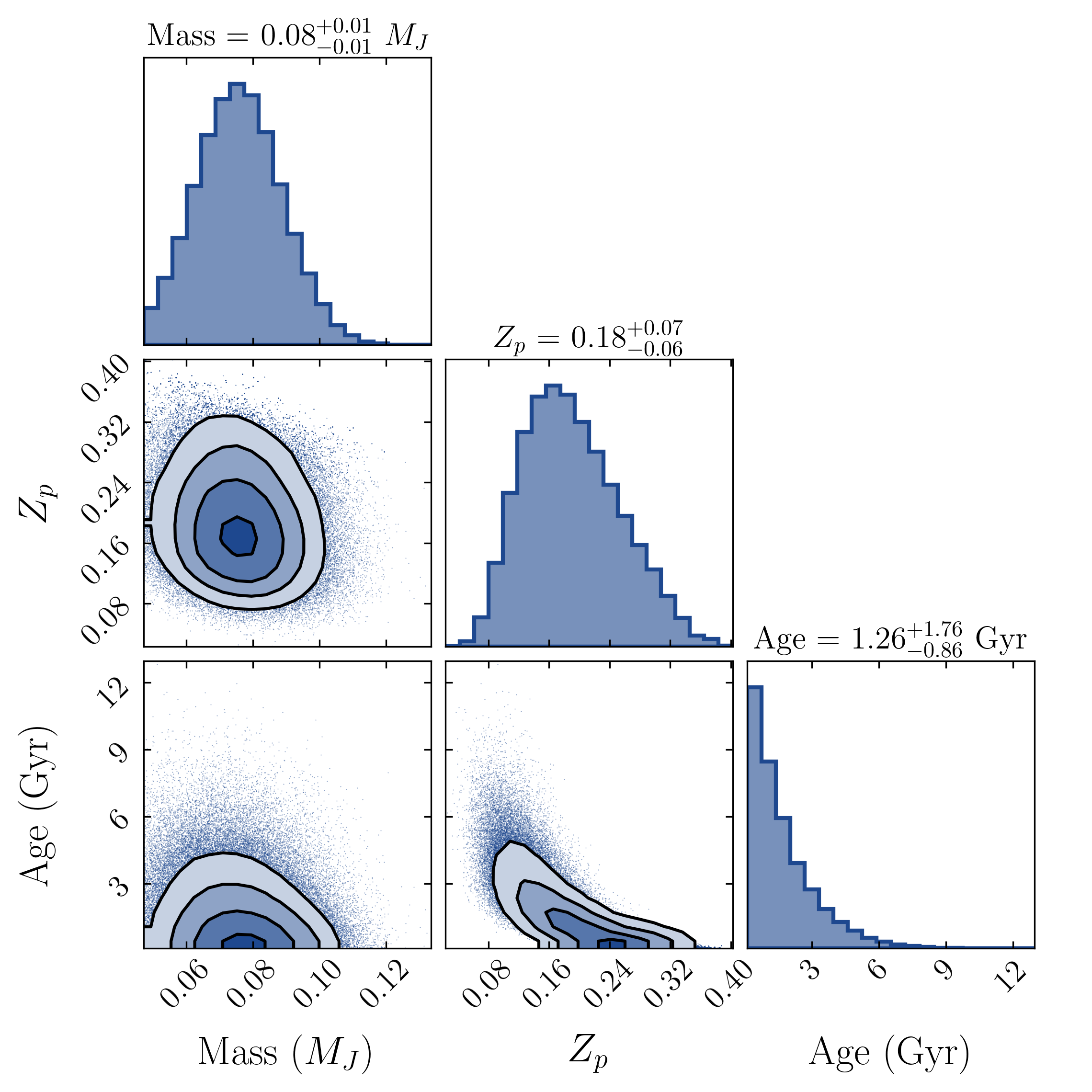
Figure 8: Posterior distributions on the planetary mass, bulk metallicity, and age from the planet evolution model described in the text.

Planets with such large envelopes despite their small cores are an interesting puzzle for core-nucleated accretion. In classic core-accretion models for planet formation, planets undergo runaway gas accretion when their cores grow to $\sim 10M_{\earth}$ (e.g. Pollack et al., 1996). TOI-1420b and WASP-107b both appear to have accreted their envelopes with $\lesssim 5M_{\earth}$ cores. Stevenson (1984) and Venturini et al. (2015) noted that runaway accretion can occur at relatively small core masses ($\lesssim 2M_{\earth}$) if the core forms water-rich beyond the ice line. On the other hand, Lee & Chiang (2016) suggest that such planets may form in “dust-free” regions of the disk, i.e. where the opacity is low and the planet can cool and accrete rapidly. Both of these scenarios require the planets to form further out before migrating inwards to their current positions. Alternatively, some investigators have proposed that the observed radii of low-density planets are inflated, either physically via tidal inflation (Millholland, 2019; Millholland et al., 2020) or because high-altitude dust and/or hazes may set the photosphere at lower pressures than otherwise expected (Kawashima et al., 2019; Wang & Dai, 2019; Gao & Zhang, 2020). Determining which (if any) of these mechanisms is at play for TOI-1420b will require more data: for instance, we could test the possibility of high-altitude dust/hazes (e.g Gao & Zhang, 2020) and tidal heating (Fortney et al., 2020) with a transmission spectrum, and additional RV observations could be used to search for a companion capable of driving the migration of TOI-1420b. Our current RV residuals are not yet sensitive to the presence of additional planets in the system. We also searched for transit-timing variations that could indicate another planet, but we found no detectable variations above a $2$ min amplitude.

5 Conclusions and Future Work

We have confirmed TOI-1420b as an exceptionally low-density planet in a 6.96 day orbit around a late G dwarf. Using data from TESS, HARPS-N, NEID, and a number of other ground-based photometric and imaging facilities, we showed that the radius of this planet is 11.9 $\pm$ 0.3 $R_{\earth}$ and the mass is 25.1 $\pm$ 3.8 $M_{\earth}$. TOI-1420b is the largest known planet with a mass less than $50M_{\earth}$, and it is similar to the planet WASP-107b in mass, radius, and irradiation. Using planetary structure models we showed that TOI-1420b has a large envelope mass fraction of 0.82${}^{+0.07}_{-0.06}$, implying a core mass of only $M_{\mathrm{core}}\sim 4M_{\earth}$.

We encourage continued RV monitoring to further constrain the system architecture, which may reveal the dynamical history of TOI-1420b. An outer companion to WASP-107b was detected only after four years of Keck/HIRES monitoring (Piaulet et al., 2021), so similar long-term investments are warranted for the TOI-1420 system. Detecting an outer companion would strengthen the argument that close-in, low-density planets like WASP-107b and TOI-1420b form further out before dynamically migrating to their present positions (Lee & Chiang, 2016). Additionally, Rossiter-McLaughlin (RM) constraints on the planet’s sky-projected obliquity can also be informative about the migration history. Large obliquities (like that observed for WASP-107b; Dai & Winn, 2017; Rubenzahl et al., 2021) may be expected for planets that underwent scattering and/or high-eccentricity migration (e.g Dawson & Johnson, 2018). The misalignment can be damped via tidal interactions with the host star (Albrecht et al., 2012), but with $a/R_{\star}>10$, TOI-1420b is unlikely to be significantly re-aligned by tides (Rice et al., 2021). Thus, if the system truly did have a dynamically-hot migration history, we may expect to observe a high obliquity. Using the upper limit on $v\sin i$ from Table 1 and the transit parameters from Table 4, the predicted RM amplitude for this system is (e.g. Triaud, 2018) $\frac{2}{3}(v\sin i_{\star})\delta\sqrt{1-b^{2}}<17$ m s^-1, well within reach for precise RV facilities assuming $v\sin i$ is close to our reported upper limit.

TOI-1420b is also an excellent target for atmospheric characterization. The planet’s atmospheric scale height $H=\frac{kT}{\mu g}$ is 1950 km (assuming $\mu=2.3$ amu), twice that of WASP-107b. TOI-1420b has a Transmission Spectroscopy Metric (TSM; Kempton et al., 2018) of 580, where we have assumed the scale factor to be 1 as the scale factors in Kempton et al. (2018) are defined only up to 10$R_{\earth}$. This puts the planet in rare company: TOI-1420b is the seventh-best exoplanet for transmission spectroscopy based on TSM, behind only WASP-107b, HD 209458b, HD 189733b, WASP-127b, KELT-11b, and WASP-69b. Low-density planets are also good targets for upper atmospheric characterization, as they are more susceptible to outflows than higher-gravity planets. We present evidence for helium in the upper atmosphere of TOI-1420b in a companion paper (Vissapragada et al. submitted).

In all, TOI-1420b presents a number of exciting future prospects for atmospheric and dynamical characterization. Comparative planetology of TOI-1420b, WASP-107b, and other similarly low-density worlds will ultimately help unveil their formation and evolution histories.

Table 5: Additional posterior values from ExoFASTv2 fit.

Parameters	Description (Units)	Posterior Values
$\gamma_{0}$	HARPS-N RV offset (m s-1)	-10327.60 ± 0.96
$\gamma_{1}$	NEID RV offset (m s-1)	-10255.2 ± 2.9
$\sigma_{\mathbf{J},0}$	HARPS-N Jitter (m s-1)	4.75 ± 0.96
$\sigma_{\mathbf{J},1}$	NEID Jitter (m s-1)	9.7 ± 3.1
$\sigma^{2}_{0}$	TESS Added Variance	-0.00000351 ± 0.00000011
$\sigma^{2}_{1}$	LCO $I$ Added Variance	0.00000725 ± 0.00000089
$\sigma^{2}_{2}$	OPM Added Variance	0.0000377 ± 0.0000061
$\sigma^{2}_{3}$	TESS Added Variance	-0.000001935 ± 0.000000087
$\sigma^{2}_{4}$	Whitin Added Variance	0.00000525 ± 0.00000080
$\sigma^{2}_{5}$	WST Added Variance	0.00000703 ± 0.00000081
$\sigma^{2}_{6}$	OAUV Added Variance	0.0000150 ± 0.0000040
$\sigma^{2}_{7}$	Calou Added Variance	0.0000114 ± 0.0000016
$\sigma^{2}_{8}$	KeplerCam Added Variance	-0.00009439 ± 0.00000061
$\sigma^{2}_{9}$	LCO $B$ Added Variance	0.00000074 ± 0.00000035
$\sigma^{2}_{10}$	LCO $g^{\prime}$ Added Variance	0.00000154 ± 0.00000035
$\sigma^{2}_{11}$	LCO $i^{\prime}$ Added Variance	0.00000281 ± 0.00000051
$\sigma^{2}_{12}$	LCO $z_{s}$ Added Variance	0.00000055 ± 0.00000029
$\sigma^{2}_{13}$	TESS Added Variance	-0.000000222 ± 0.000000096
$\sigma^{2}_{14}$	TESS Added Variance	-0.000000048 ± 0.000000098
$\sigma^{2}_{15}$	TESS Added Variance	-0.000000090 ± 0.000000088
$u_{1,0}$	$B$ Quadratic Limb Darkening	0.756 ± 0.036
$u_{2,0}$	$B$ Quadratic Limb Darkening	0.070 ± 0.037
$u_{1,1}$	$I$ Quadratic Limb Darkening	0.345 ± 0.036
$u_{2,1}$	$I$ Quadratic Limb Darkening	0.266 ± 0.035
$u_{1,2}$	$g^{\prime}$ Quadratic Limb Darkening	0.671 ± 0.044
$u_{2,2}$	$g^{\prime}$ Quadratic Limb Darkening	0.122 ± 0.052
$u_{1,3}$	$i^{\prime}$ Quadratic Limb Darkening	0.345 ± 0.034
$u_{2,3}$	$i^{\prime}$ Quadratic Limb Darkening	0.235 ± 0.035
$u_{1,4}$	$z_{s}$ Quadratic Limb Darkening	0.291 ± 0.033
$u_{2,4}$	$z_{s}$ Quadratic Limb Darkening	0.257 ± 0.033
$u_{1,5}$	TESS Quadratic Limb Darkening	0.356 ± 0.022
$u_{2,5}$	TESS Quadratic Limb Darkening	0.243 ± 0.023

References

- Agol et al. (2020) Agol, E., Luger, R., & Foreman-Mackey, D. 2020, AJ, 159, 123
- Akeson et al. (2013) Akeson, R. L., Chen, X., Ciardi, D., et al. 2013, PASP, 125, 989
- Albrecht et al. (2012) Albrecht, S., Winn, J. N., Johnson, J. A., et al. 2012, ApJ, 757, 18
- Anderson et al. (2017) Anderson, D. R., Collier Cameron, A., Delrez, L., et al. 2017, A&A, 604, A110
- Astropy Collaboration et al. (2013) Astropy Collaboration, Robitaille, T. P., Tollerud, E. J., et al. 2013, A&A, 558, A33
- Astropy Collaboration et al. (2018) Astropy Collaboration, Price-Whelan, A. M., Sipőcz, B. M., et al. 2018, AJ, 156, 123
- Barkaoui et al. (2023) Barkaoui, K., Pozuelos, F. J., Hellier, C., et al. 2023, arXiv e-prints, arXiv:2307.08350
- Bieryla et al. (2021) Bieryla, A., Tronsgaard, R., Buchhave, L. A., et al. 2021, in Posters from the TESS Science Conference II (TSC2, 124
- Borucki et al. (2010) Borucki, W. J., Koch, D., Basri, G., et al. 2010, Science, 327, 977
- Brown et al. (2013) Brown, T. M., Baliber, N., Bianco, F. B., et al. 2013, PASP, 125, 1031
- Buchhave et al. (2012) Buchhave, L. A., Latham, D. W., Johansen, A., et al. 2012, Nature, 486, 375
- Chabrier et al. (2019) Chabrier, G., Mazevet, S., & Soubiran, F. 2019, ApJ, 872, 51
- Ciardi et al. (2015) Ciardi, D. R., Beichman, C. A., Horch, E. P., & Howell, S. B. 2015, ApJ, 805, 16
- Collins (2019) Collins, K. 2019, in American Astronomical Society Meeting Abstracts, Vol. 233, American Astronomical Society Meeting Abstracts #233, 140.05
- Collins et al. (2017) Collins, K. A., Kielkopf, J. F., Stassun, K. G., & Hessman, F. V. 2017, AJ, 153, 77
- Cosentino et al. (2012) Cosentino, R., Lovis, C., Pepe, F., et al. 2012, in Society of Photo-Optical Instrumentation Engineers (SPIE) Conference Series, Vol. 8446, Ground-based and Airborne Instrumentation for Astronomy IV, ed. I. S. McLean, S. K. Ramsay, & H. Takami, 84461V
- Cosentino et al. (2014) Cosentino, R., Lovis, C., Pepe, F., et al. 2014, in Society of Photo-Optical Instrumentation Engineers (SPIE) Conference Series, Vol. 9147, Ground-based and Airborne Instrumentation for Astronomy V, ed. S. K. Ramsay, I. S. McLean, & H. Takami, 91478C
- Cutri et al. (2003) Cutri, R. M., Skrutskie, M. F., van Dyk, S., et al. 2003, VizieR Online Data Catalog, II/246
- Cutri et al. (2021) Cutri, R. M., Wright, E. L., Conrow, T., et al. 2021, VizieR Online Data Catalog, II/328
- Dai & Winn (2017) Dai, F., & Winn, J. N. 2017, AJ, 153, 205
- Dawson & Johnson (2018) Dawson, R. I., & Johnson, J. A. 2018, ARA&A, 56, 175
- Dumusque (2018) Dumusque, X. 2018, A&A, 620, A47
- Eastman et al. (2019) Eastman, J. D., Rodriguez, J. E., Agol, E., et al. 2019, arXiv e-prints, arXiv:1907.09480
- Foreman-Mackey et al. (2021) Foreman-Mackey, D., Luger, R., Agol, E., et al. 2021, arXiv e-prints, arXiv:2105.01994
- Foreman-Mackey et al. (2021) Foreman-Mackey, D., Savel, A., Luger, R., et al. 2021, exoplanet-dev/exoplanet v0.5.1, , , doi:10.5281/zenodo.1998447. https://doi.org/10.5281/zenodo.1998447
- Foreman-Mackey et al. (2021) Foreman-Mackey, D., Luger, R., Agol, E., et al. 2021, arXiv e-prints, arXiv:2105.01994
- Fortney et al. (2021) Fortney, J. J., Dawson, R. I., & Komacek, T. D. 2021, Journal of Geophysical Research (Planets), 126, e06629
- Fortney et al. (2020) Fortney, J. J., Visscher, C., Marley, M. S., et al. 2020, AJ, 160, 288
- Gaia Collaboration et al. (2022) Gaia Collaboration, Vallenari, A., Brown, A. G. A., et al. 2022, arXiv e-prints, arXiv:2208.00211
- Gao & Zhang (2020) Gao, P., & Zhang, X. 2020, ApJ, 890, 93
- Gelman & Rubin (1992) Gelman, A., & Rubin, D. B. 1992, Statistical Science, 7, 457 . https://doi.org/10.1214/ss/1177011136
- Guerrero et al. (2021) Guerrero, N. M., Seager, S., Huang, C. X., et al. 2021, ApJS, 254, 39
- Halverson et al. (2016) Halverson, S., Terrien, R., Mahadevan, S., et al. 2016, in Society of Photo-Optical Instrumentation Engineers (SPIE) Conference Series, Vol. 9908, Ground-based and Airborne Instrumentation for Astronomy VI, ed. C. J. Evans, L. Simard, & H. Takami, 99086P
- Harris et al. (2020) Harris, C. R., Millman, K. J., van der Walt, S. J., et al. 2020, Nature, 585, 357
- Hedges et al. (2020) Hedges, C., Angus, R., Barentsen, G., et al. 2020, Research Notes of the American Astronomical Society, 4, 220
- Hodapp et al. (2003) Hodapp, K. W., Jensen, J. B., Irwin, E. M., et al. 2003, PASP, 115, 1388
- Høg et al. (2000) Høg, E., Fabricius, C., Makarov, V. V., et al. 2000, A&A, 355, L27
- Jenkins (2002) Jenkins, J. M. 2002, ApJ, 575, 493
- Jenkins et al. (2010) Jenkins, J. M., Caldwell, D. A., Chandrasekaran, H., et al. 2010, ApJ, 713, L87
- Jenkins et al. (2016) Jenkins, J. M., Twicken, J. D., McCauliff, S., et al. 2016, in Society of Photo-Optical Instrumentation Engineers (SPIE) Conference Series, Vol. 9913, Software and Cyberinfrastructure for Astronomy IV, ed. G. Chiozzi & J. C. Guzman, 99133E
- Jensen (2013) Jensen, E. 2013, Tapir: A web interface for transit/eclipse observability, Astrophysics Source Code Library, , , ascl:1306.007
- Kanodia et al. (2018) Kanodia, S., Mahadevan, S., Ramsey, L. W., et al. 2018, in Society of Photo-Optical Instrumentation Engineers (SPIE) Conference Series, Vol. 10702, Ground-based and Airborne Instrumentation for Astronomy VII, ed. C. J. Evans, L. Simard, & H. Takami, 107026Q
- Kawashima et al. (2019) Kawashima, Y., Hu, R., & Ikoma, M. 2019, ApJ, 876, L5
- Kempton et al. (2018) Kempton, E. M. R., Bean, J. L., Louie, D. R., et al. 2018, PASP, 130, 114401
- Kipping (2013) Kipping, D. M. 2013, MNRAS, 435, 2152
- Kochanek et al. (2017) Kochanek, C. S., Shappee, B. J., Stanek, K. Z., et al. 2017, PASP, 129, 104502
- Kreidberg et al. (2018) Kreidberg, L., Line, M. R., Thorngren, D., Morley, C. V., & Stevenson, K. B. 2018, ApJ, 858, L6
- Kumar et al. (2019) Kumar, R., Carroll, C., Hartikainen, A., & Martin, O. A. 2019, The Journal of Open Source Software, doi:10.21105/joss.01143. http://joss.theoj.org/papers/10.21105/joss.01143
- Lam et al. (2017) Lam, K. W. F., Faedi, F., Brown, D. J. A., et al. 2017, A&A, 599, A3
- Latham et al. (2011) Latham, D. W., Rowe, J. F., Quinn, S. N., et al. 2011, ApJ, 732, L24
- Lee (2019) Lee, E. J. 2019, ApJ, 878, 36
- Lee & Chiang (2016) Lee, E. J., & Chiang, E. 2016, ApJ, 817, 90
- Li et al. (2019) Li, J., Tenenbaum, P., Twicken, J. D., et al. 2019, PASP, 131, 024506
- Lightkurve Collaboration et al. (2018) Lightkurve Collaboration, Cardoso, J. V. d. M., Hedges, C., et al. 2018, Lightkurve: Kepler and TESS time series analysis in Python, Astrophysics Source Code Library, , , ascl:1812.013
- Lindegren et al. (2021) Lindegren, L., Bastian, U., Biermann, M., et al. 2021, A&A, 649, A4
- Lopez & Fortney (2014) Lopez, E. D., & Fortney, J. J. 2014, ApJ, 792, 1
- Luger et al. (2019) Luger, R., Agol, E., Foreman-Mackey, D., et al. 2019, AJ, 157, 64
- Mayor & Queloz (1995) Mayor, M., & Queloz, D. 1995, Nature, 378, 355
- McCully et al. (2018a) McCully, C., Volgenau, N. H., Harbeck, D.-R., et al. 2018a, in Society of Photo-Optical Instrumentation Engineers (SPIE) Conference Series, Vol. 10707, Proc. SPIE, 107070K
- McCully et al. (2018b) McCully, C., Turner, M., H., V. N., et al. 2018b, LCOGT/banzai: Initial Release, v0.9.4, Zenodo, doi:10.5281/zenodo.1257560. https://doi.org/10.5281/zenodo.1257560
- McKee & Montet (2022) McKee, B. J., & Montet, B. T. 2022, arXiv e-prints, arXiv:2212.07450
- Miller & Fortney (2011) Miller, N., & Fortney, J. J. 2011, ApJ, 736, L29
- Millholland (2019) Millholland, S. 2019, ApJ, 886, 72
- Millholland et al. (2020) Millholland, S., Petigura, E., & Batygin, K. 2020, ApJ, 897, 7
- Ohta et al. (2005) Ohta, Y., Taruya, A., & Suto, Y. 2005, ApJ, 622, 1118
- Pepe et al. (2002) Pepe, F., Mayor, M., Galland, F., et al. 2002, A&A, 388, 632
- Pepper et al. (2017) Pepper, J., Rodriguez, J. E., Collins, K. A., et al. 2017, AJ, 153, 215
- Petigura et al. (2017) Petigura, E. A., Sinukoff, E., Lopez, E. D., et al. 2017, AJ, 153, 142
- Petigura et al. (2018) Petigura, E. A., Marcy, G. W., Winn, J. N., et al. 2018, AJ, 155, 89
- Piaulet et al. (2021) Piaulet, C., Benneke, B., Rubenzahl, R. A., et al. 2021, AJ, 161, 70
- Pollack et al. (1996) Pollack, J. B., Hubickyj, O., Bodenheimer, P., et al. 1996, Icarus, 124, 62
- Prša et al. (2022) Prša, A., Kochoska, A., Conroy, K. E., et al. 2022, ApJS, 258, 16
- Rice et al. (2021) Rice, M., Wang, S., Howard, A. W., et al. 2021, AJ, 162, 182
- Ricker et al. (2015) Ricker, G. R., Winn, J. N., Vanderspek, R., et al. 2015, Journal of Astronomical Telescopes, Instruments, and Systems, 1, 014003
- Robertson et al. (2019) Robertson, P., Anderson, T., Stefansson, G., et al. 2019, Journal of Astronomical Telescopes, Instruments, and Systems, 5, 015003
- Rubenzahl et al. (2021) Rubenzahl, R. A., Dai, F., Howard, A. W., et al. 2021, AJ, 161, 119
- Safonov et al. (2017) Safonov, B. S., Lysenko, P. A., & Dodin, A. V. 2017, Astronomy Letters, 43, 344
- Salvatier et al. (2016) Salvatier, J., Wiecki, T. V., & Fonnesbeck, C. 2016, PeerJ Computer Science, 2, e55
- Schwab et al. (2016) Schwab, C., Rakich, A., Gong, Q., et al. 2016, in Society of Photo-Optical Instrumentation Engineers (SPIE) Conference Series, Vol. 9908, Ground-based and Airborne Instrumentation for Astronomy VI, ed. C. J. Evans, L. Simard, & H. Takami, 99087H
- Shappee et al. (2014) Shappee, B. J., Prieto, J. L., Grupe, D., et al. 2014, ApJ, 788, 48
- Smith et al. (2012) Smith, J. C., Stumpe, M. C., Van Cleve, J. E., et al. 2012, PASP, 124, 1000
- Spake et al. (2018) Spake, J. J., Sing, D. K., Evans, T. M., et al. 2018, Nature, 557, 68
- Stassun et al. (2018) Stassun, K. G., Oelkers, R. J., Pepper, J., et al. 2018, AJ, 156, 102
- Stefansson et al. (2016) Stefansson, G., Hearty, F., Robertson, P., et al. 2016, ApJ, 833, 175
- Stefànsson et al. (2022) Stefànsson, G., Mahadevan, S., Petrovich, C., et al. 2022, ApJ, 931, L15
- Stevenson (1984) Stevenson, D. J. 1984, in Lunar and Planetary Science Conference, Lunar and Planetary Science Conference, 822–823
- Stumpe et al. (2014) Stumpe, M. C., Smith, J. C., Catanzarite, J. H., et al. 2014, PASP, 126, 100
- Stumpe et al. (2012) Stumpe, M. C., Smith, J. C., Van Cleve, J. E., et al. 2012, PASP, 124, 985
- Szentgyorgyi & Furész (2007) Szentgyorgyi, A. H., & Furész, G. 2007, in Revista Mexicana de Astronomia y Astrofisica Conference Series, Vol. 28, Revista Mexicana de Astronomia y Astrofisica Conference Series, ed. S. Kurtz, 129–133
- Theano Development Team (2016) Theano Development Team. 2016, arXiv e-prints, abs/1605.02688. http://arxiv.org/abs/1605.02688
- Thorngren & Fortney (2019) Thorngren, D., & Fortney, J. J. 2019, ApJ, 874, L31
- Thorngren et al. (2016) Thorngren, D. P., Fortney, J. J., Murray-Clay, R. A., & Lopez, E. D. 2016, ApJ, 831, 64
- Triaud (2018) Triaud, A. H. M. J. 2018, in Handbook of Exoplanets, ed. H. J. Deeg & J. A. Belmonte, 2
- Twicken et al. (2018) Twicken, J. D., Catanzarite, J. H., Clarke, B. D., et al. 2018, PASP, 130, 064502
- Venturini et al. (2015) Venturini, J., Alibert, Y., Benz, W., & Ikoma, M. 2015, A&A, 576, A114
- Virtanen et al. (2020) Virtanen, P., Gommers, R., Oliphant, T. E., et al. 2020, Nature Methods, 17, 261
- Wang & Dai (2019) Wang, L., & Dai, F. 2019, ApJ, 873, L1
- Zechmeister et al. (2018) Zechmeister, M., Reiners, A., Amado, P. J., et al. 2018, A&A, 609, A12