Holographic Limitations and Corrections to Quantum Information Protocols

Abstract

We discuss the limitations imposed on entanglement distribution, quantum teleportation, and quantum communication by holographic bounds, such as the Bekenstein bound and Susskind’s spherical entropy bound. For continuous-variable (CV) quantum information, we show how the naive application of holographic corrections disrupts well-established results. These corrections render perfect CV teleportation impossible, preclude uniform convergence in the teleportation simulation of lossy quantum channels, and impose a revised PLOB bound for quantum communication. While these mathematical corrections do not immediately impact practical quantum technologies, they are critical for a deeper theoretical understanding of quantum information theory.

I Introduction

Inspired by the holographic principle, the holographic bounds [1] set fundamental limits on the amount of information that can be contained within a given volume of space. Rooted in theories that intersect quantum mechanics, general relativity, and thermodynamics, these bounds suggest that the maximum entropy in a spatial region is directly proportional to its surface area, rather than its volume. Prominent examples include the Bekenstein Bound [2], Susskind’s spherical entropy bound [3], and the Bekenstein-Hawking entropy formula for black holes [4, 5]. These have profound implications for our understanding of gravity, information theory, and the fabric of the universe itself.

It is very interesting to explore such bounds in the context of quantum information theory. Assuming a simple connection between thermodynamic and von Neumann entropy [6], and assuming that quantum protocols can be operated in the same way no matter if in flat or curved space-time, one can derive simple limitations for the number of qubits that can be entangled or teleported over a certain distance. More interesting, because standard results in continuous-variable (CV) quantum information are related to high-entropy limits, the direct application of the holographic bounds to CV protocols leads to fundamental restrictions and corrections. This is the case for CV teleportation [7, 8], its associated tools for quantum channel simulation [9, 10], and also for the fundamental limit of quantum communication, known as the Pirandola-Laurenza-Ottaviani-Banchi (PLOB) bound [11].

II General scenario

Consider an entanglement source between two parties, Alice and Bob. As shown in Fig. 1, the source is located at the origin $x=0$ while Alice is at position $x=-R-\varepsilon$ and Bob at $x=R+\varepsilon$ with $\varepsilon\geq 0$ arbitrarily small. Alice-Bob distance is therefore equal to $D=2R+2\varepsilon\geq 2R$. Suppose that the source distributes a maximally entangled state $\Psi_{AB}:=|\Psi\rangle_{AB}\langle\Psi|$ where $|\Psi\rangle_{AB}=d^{-1/2}\sum_{i}|ii\rangle$ with $d$ being the local dimension of systems $A$ (reaching Alice) and $B$ (reaching Bob). Because of entanglement distillation, this state is equivalent to $n=\mathrm{log}_{2}d$ Bell pairs or entanglement bits (ebits), i.e., $n$ copies of the state $|\Psi_{0}\rangle=2^{-1/2}(|00\rangle+|11\rangle)$. This resource may be used to implement quantum protocols, including teleportation.

Using this shared distilled resource, Alice may teleport an arbitrary state of $n$ qubits to Bob. She may measure each input qubit (in a reduced state $\rho$) with the $A$-part of an ebit by performing a joint Bell detection. The effect of the measurement is to project Bob’s $B$-part of the same ebit onto the state $P_{u}\rho P_{u}^{\dagger}$, where $\{P_{u}\}_{u=0}^{3}=\{I,X,Y,Z\}$ is the set of Pauli operators [6] plus the identity. Then, Alice transmits the 2-bit value $u$ to Bob. Thanks to this classical communication (CC), Bob can undo the unitary $P_{u}$ from his $B$ qubit, thus reconstructing the state of Alice’s input qubit. This procedure can be repeated for all the $n$ input qubits, so that Alice’s global state is perfectly transferred to Bob’s qubits. For this transfer, $n$ ebits are consumed and $2n$ classical bits need to be communicated. It is natural to assume that input qubits and shared ebits are of the same nature (e.g., same mass). Here we refer to $D\simeq 2R$ as to entanglement or teleportation distance.

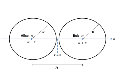
Figure 1: Double-sphere scenario. An entanglement source is located at the origin $x=0$ of the position coordinate $x$, while Alice is at $-R-\varepsilon$ and Bob at $R+\varepsilon$, with $\varepsilon$ arbitrarily small. Alice’s and Bob’s local labs are within spheres of radius $R$. The middle source distributes $n$ Bell pairs to the remote parties, separated by $D=2R+2\varepsilon\simeq 2R$. We call $D$ entanglement or teleportation distance.

Because the non-local state $\Psi_{AB}$ is pure, it has von Neumann entropy $S_{AB}=0$. At the same time, the reduced local states of Alice and Bob are maximally mixed, i.e., $\rho_{A}=\rho_{B}=d^{-1}I$ where $I$ is the identity operator. Thus, in Alice’s and Bob’s labs, the local systems have maximal von Neumann entropy $S_{A}=S_{B}=n$ qubits. This is also known as entanglement entropy.

For the following derivations, we make the following naive assumptions:

• The von Neumann entropy of a subsystem provides its thermodynamic entropy. More precisely, we assume that the thermodynamic entropy is obtained by changing the log-base to nats and including the Boltzmann constant $k$, so that $S_{A}^{\mathrm{th}}=S_{B}^{\mathrm{th}}=kn\ln 2$.

• Quantum protocols for entanglement distribution, teleportation, and quantum communication are assumed to be operated in the same way no matter if they are in flat or curved space-time.

III Holographic bounds

Given the assumptions above one can easily show the immediate and general limitations that holographic bounds impose on protocols for entanglement distribution and quantum teleportation. These limitations are expressed in terms of the number of ebits that can be distributed or qubits that can be teleported over some distance $D$. We discuss these limitations from the perspective of the Bekenstein bound [2], and we then extend the discussion to Susskind’s spherical bound [3].

III.1 Holographic limits from the Bekenstein bound

The Bekenstein bound holds for any weakly gravitating matter system in an asymptotically flat space-time. In such an approximately flat scenario, consider a single sphere of radius $R$ centered on Alice’s local system $A$ (e.g., see the left sphere of Fig. 1). The thermodynamic entropy of Alice’s system must satisfy the bound [2]

$$S_{A}^{\mathrm{th}}(=kn\ln 2)\leq\frac{2\pi kRE}{\hbar c},$$ (1)

where $E$ is the energy within the sphere, $\hbar$ is the Planck constant, and $c$ is the speed of light in vacuum. It is easy to see that this inequality provides a macroscopic upper bound to the number $n$ of qubits that can be compressed within a sphere of radius $R$ and internal energy $E$.

Because $D\geq 2R$, we may write

$$DE\geq\frac{\hbar c\ln 2}{\pi}n\simeq 6.97\times 10^{-27}n~{}~{}~{}\mathrm{[J\cdot m]}.$$ (2)

This can be seen as an upper bound on the number of ebits that can be shared by two parties that are separated by $D$ and have local energy $E$ (as depicted in the two-sphere scenario of Fig. 1). In turn, this is also an upper bound on the number of qubits that can be teleported over distance $D$ by consuming an entanglement source with total energy $2E$ [12].

Now assume that the local systems $A$ and $B$ in Fig. 1 are at rest, so that their local mass $M$ provides an equivalent energy of $E=Mc^{2}$ (we assume there is no charge or momentum associated with the qubits, so we also ignore relativistic effects). Then, Eq. (2) becomes

$$DM\geq\frac{\hbar\ln 2}{\pi c}n\simeq 7.77\times 10^{-44}n~{}~{}~{}\mathrm{[m\cdot Kg/s]},$$ (3)

which provides a macroscopic bound to the number $n$ of qubits that can be entangled at distance $D$ with local mass $M$. If we assume that $M$ is also the mass of an object to be teleported (in a mass-preserving teleportation), then Eq. (3) bounds the number $n$ of massive qubits that can be teleported over distance $D$. It is clear that, fixing the number $n$ of qubits in Eq. (3), we get a trade-off between entanglement/teleportation distance $D$ and local mass $M$. Surprisingly, the lesser $M$ is, the greater $D$ needs to be, so that we can entangle or teleport massive objects only beyond a minimum distance, which becomes infinite in the limit of $M\rightarrow 0$.

III.2 Limitations from the spherical entropy bound

The violation of the Bekenstein bound is associated with a violation of the second law of thermodynamics. It is generally considered to be valid for weakly gravitating systems in spherical symmetry [1]. Under the same kind of symmetry, one may consider Susskind’s spherical entropy bound [3] which can be extended to strongly gravitating systems, i.e., truly curved space-time.

The thermodynamic entropy in a volume of space bounded by a spherical surface with area $\mathcal{A}=4\pi R^{2}$ and radius $R$ must satisfy the bound

$$S^{\mathrm{th}}\leq\frac{k\mathcal{A}}{4l_{p}^{2}}=\frac{\pi kR^{2}}{l_{p}^{2}},$$ (4)

where $l_{p}=\sqrt{G\hbar/c^{3}}\simeq 1.6\times 10^{-35}$m is the Planck length, with $G$ being the gravitational constant. The saturation of this bound is achieved by the most entropic possible object, a black hole. This extremal value is also known as Bekenstein-Hawking (BH) entropy $S_{\mathrm{BH}}$, in which case $R$ and $\mathcal{A}$ are radius and area of the event horizon, respectively. In the absence of charge and angular momentum, we may consider a Schwarzschild black hole with mass $M$ whose event horizon has radius $R_{\text{S}}=2GM/c^{2}$. Then the BH entropy becomes

$$S_{\mathrm{BH}}=\frac{\pi kR_{\text{S}}^{2}}{l_{p}^{2}}=\frac{2\pi kcR_{\text{S}}M}{\hbar}.$$ (5)

In our entanglement distribution scenario (see Fig. 1), Alice’s and Bob’s local systems have $S_{A}^{\mathrm{th}}=S_{B}^{\mathrm{th}}=kn\ln 2$, so the entropy bound in Eq. (4) directly provides

$$n\leq\frac{\pi}{\ln 2}(R/l_{p})^{2},~{}~{}\frac{D}{l_{p}}\geq\sqrt{\frac{4\ln 2}{\pi}n}~{}~{}.$$ (6)

Thus, independently of their mass, the maximum number $n$ of qubits that can be entangled or teleported between Alice and Bob is limited by the area of the circle $\pi R^{2}$ in Planck units. Similarly, there is a universal minimum distance $D/l_{p}$ for $n$-qubit entanglement and teleportation that scales quadratically in the number of qubits [13].

Note that tighter restrictions can be derived from the ‘t Hooft bound for ordinary matter [14, 15]. If we exclude energies leading to gravitational collapse and assume an approximately flat spacetime, the maximum thermodynamic entropy within a sphere with area $\mathcal{A}$ scales as $S^{\mathrm{th}}\lesssim k(\mathcal{A}/l_{p}^{2})^{3/4}$. Replacing $S^{\mathrm{th}}=kn\ln 2$, we then find

$$n\lesssim(R/l_{p})^{3/2},~{}~{}\frac{D}{l_{p}}\gtrsim n^{2/3}.$$ (7)

These scalings are clearly tighter than those in Eq. (6).

III.3 Black-hole creation dynamics

For the sake of completeness, let us describe the previous process by setting equality in Eq. (3), so that $D_{\text{min}}M=n\hbar\ln 2/(\pi c)$. This is equivalent to say that we are considering the smallest spheres capable of enclosing Alice’s and Bob’s systems. By increasing the local mass $M$, the entanglement/teleportation distance $D_{\text{min}}$ decreases. Simultaneously, the Schwarzschild radius associated with Alice’s and Bob’s systems increases as $R_{\text{S}}=2GM/c^{2}$. At the critical point $D_{\text{min}}=2R_{\text{S}}$, Alice’s and Bob’s systems become a pair of entangled black holes whose event horizons are tangent. Clearly, teleportation can no longer work because the CC needed to perform the protocol cannot escape the horizons.

One can easily check that, at the critical point, the local masses must be equal to

$$\frac{{M}}{{m_{p}}}=\sqrt{\frac{n\ln 2}{4\pi}},$$ (8)

where $m_{p}=\sqrt{\hbar c/G}\simeq 21.76$$\mu$g is the Planck mass. It is then easy to see that the minimum distance is $D_{\text{min}}/l_{p}=\sqrt{4n\ln 2/\pi}$, which saturates the bound in Eq. (6). For $D>D_{\text{min}}$, $n$-qubit protocols for entanglement distribution and teleportation become in principle possible because Alice’s and Bob’s labs can be located outside the event horizons within their local spheres.

IV Holographic limitations to CV protocols

Let us now show what type of implications and limitations the spherical bound would have for continuous-variable (CV) quantum information. This is a field where a number of fundamental results are obtained by taking limits for infinite entanglement, squeezing or modulation, which means that these limits imply infinite entropy.

IV.1 Limits to Gaussian modulation and two-mode squeezing

Let us start from the problem of signal modulation. In a typical CV protocol for quantum communication, Alice prepares an input alphabet of coherent states whose amplitude $\alpha$ is modulated according to a Gaussian distribution. On average this is a thermal state with $\bar{n}$ mean number of photons and entropy

$$h(\bar{n}):=(\bar{n}+1)\log_{2}(\bar{n}+1)-\bar{n}\log_{2}\bar{n}.$$ (9)

It is easy to show that $h(\bar{n})\geq\log_{2}(e\bar{n})$ so that, multiplying by $\ln 2$ and including the Boltzmann constant $k$, we compute Alice’s thermodynamic entropy $S_{A}^{\mathrm{th}}\geq k\ln(e\bar{n})$. Using the latter inequality in the spherical bound of Eq. (4) leads to

$$\bar{n}\leq e^{\pi R_{p}^{2}-1},$$ (10)

where $R_{p}:=R/l_{p}$ is the radius in Planck units. The first immediate consequence of Eq. (10) is that Alice’s signal alphabet must be limited by her radius, so that infinite modulation is not allowed for any finite $R_{p}$.

The same bound clearly holds for the maximal amount of CV entanglement that can be shared by Alice and Bob. The fundamental state to consider here is the two-mode squeezed vacuum (TMSV) state $\Phi_{AB}^{\mu}$ with parameter $\mu=\bar{n}+1/2$. Tracing out Bob’s $B$-part of this state provides Alice with a local thermal state $\rho_{A}^{\bar{n}}$ with $\bar{n}=\mu-1/2$ mean photons. Therefore Alice’s reduced state has thermodynamic entropy $S_{A}^{\mathrm{th}}\geq k\ln(e\bar{n})$ and the spherical bound provides Eq. (10) or, equivalently,

$$\mu\leq\mu_{\max}(R_{p}):=e^{\pi R_{p}^{2}-1}+1/2.$$ (11)

As we will see below, the bound in Eq. (11) has drastic consequences for CV teleportation [7, 8] and the teleportation simulation of channels [11]. It will also impose holographic corrections to the quantum capacities of bosonic channels [16].

IV.2 Holographic no-go for ideal CV teleportation

Let us apply the CV teleportation protocol to mode $a$ of an input TMSV state $\Phi_{Ca}^{\tilde{\mu}}$ by using another TMSV state $\Phi_{AB}^{\mu}$ as a resource. The ideal CV Bell detection on modes $a$ and $A$, and the CC of the outcome realizes an approximate identity channel $\mathcal{I}_{a\rightarrow B}^{\mu}$ from mode $a$ to mode $B$. This is strongly (i.e., point-wise) equivalent to an additive-noise Gaussian channel with added noise [17, 18, 19, 20]

$$\xi=2\mu-\sqrt{4\mu^{2}-1}.$$ (12)

When applied to $\Phi_{Ca}^{\tilde{\mu}}$, we get the output $\Phi_{CB}^{\mu,\tilde{\mu}}:=\mathcal{I}_{C}\otimes\mathcal{I}_{a\rightarrow B}^{\mu}(\Phi_{Ca}^{\tilde{\mu}})$ where $\mathcal{I}_{C}$ is the identity channel applied to system $C$. Consider the (square-root) quantum fidelity

$$F(\mu,\tilde{\mu})=\left\|\sqrt{\Phi_{Ca}^{\tilde{\mu}}}\sqrt{\Phi_{CB}^{\mu,\tilde{\mu}}}\right\|_{1}$$ (13)

between the input and the output (teleported) state, where $||O||_{1}:=\mathrm{Tr}\sqrt{O^{\dagger}O}$ is the trace norm. In the present case, this is the fidelity of teleporting CV entanglement [21]. Using the formula for Gaussian states [22], we explicitly compute (see also Ref. [9, App. A])

$$F(\mu,\tilde{\mu})=\left\{1-4\tilde{\mu}\left[\sqrt{4\mu^{2}-1}+\tilde{\mu}-2\mu\left(1+2\tilde{\mu}\xi\right)\right]\right\}^{-1/4}.$$ (14)

This expression would go to 1 if we could take the limit of $\mu\rightarrow+\infty$ but, unfortunately, we have the holographic bound $\mu\leq\mu_{\max}(R_{p})$ of Eq. (11) for any radius $R_{p}$. This implies $F<1$ for any finite $R_{p}$, so we cannot perfectly teleport CV entanglement. The maximum fidelity in Eq. (14) is achieved for $\tilde{\mu}=1/2$, corresponding to the teleportation of the vacuum state from $a$ to $B$. At Planckian distance $R_{p}=1$, we have maximal fidelity $F\simeq 0.986403$. At larger $R_{p}$, the fidelity approaches $1$ but remains $<1$ at any finite radius.

This reasoning implies that CV teleportation would not strongly converge to the identity channel unless Alice and Bob are separated by an infinite distance. Note that this problem affects not only the strong convergence but also the uniform convergence of CV teleportation [9, 10].

IV.3 No uniform convergence in teleportation simulation

Because the holographic bounds implies that CV teleportation cannot be perfect at finite distance, we have that many applications of this tool are also affected. This includes the teleportation simulation of bosonic Gaussian channels. To illustrate the idea consider the bosonic pure-loss channel which is the most relevant Gaussian channel. This may be represented by a beam splitter with transmissivity $0<\eta<1$ which mixes an incoming bosonic mode with an environmental vacuum mode.

Because the pure-loss channel $\mathcal{E}_{\eta}$ is teleportation covariant [11], it may be simulated by using the CV teleportation protocol $\mathcal{T}$ implemented over its quasi-Choi matrix $\chi_{\eta}^{\mu}:=\mathcal{I}_{A}\otimes\mathcal{E}_{\eta}(\Phi_{AB}^{\mu})$. In other words, we may write the simulation channel $\mathcal{E}_{\eta}^{\mu}(\rho):=\mathcal{T}(\rho\otimes\chi_{\eta}^{\mu})$ for any input state $\rho$. One can check that $\mathcal{E}_{\eta}^{\mu}=\mathcal{E}_{\eta}\circ\mathcal{I}^{\mu}$ and write

$$\lim_{\mu\rightarrow\infty}\left\|\mathcal{E}_{\eta}-\mathcal{E}_{\eta}^{\mu}\right\|_{\diamond}=0.$$ (15)

Recall that the diamond distance is the appropriate distance between channels and defined by the following optimization of the trace distance over bipartite states $\rho_{AB}$

$$\left\|\mathcal{E}_{\eta}-\mathcal{E}_{\eta}^{\mu}\right\|_{\diamond}:=\sup_{\rho_{AB}}\left\|\mathcal{I}_{A}\otimes\mathcal{E}_{\eta}(\rho_{AB})-\mathcal{I}_{A}\otimes\mathcal{E}_{\eta}^{\mu}(\rho_{AB})\right\|_{1}.$$ (16)

Holographically, we cannot take the limit in Eq. (15) due to Eq. (11), so that the uniform convergence is excluded by a non-zero lower bound. In fact, we have

$$\left\|\mathcal{E}_{\eta}-\mathcal{E}_{\eta}^{\mu}\right\|_{\diamond}\overset{(1)}{\geq}\left\|\left|00\right\rangle\left\langle 00\right|-\left|0\right\rangle\left\langle 0\right|\otimes\mathcal{E}_{\eta}^{\mu}(\left|0\right\rangle\left\langle 0\right|)\right\|_{1}$$

$$\overset{(2)}{\geq}2[1-\left\langle 0\right|\mathcal{E}_{\eta}^{\mu}(\left|0\right\rangle\left\langle 0\right|)\left|0\right\rangle]$$

$$\overset{(3)}{=}2\eta\xi(1+\eta\xi)^{-1},$$ (17)

where: (1) we pick a particular state (the vacuum $\rho_{AB}=\rho_{00}:=\left|00\right\rangle\left\langle 00\right|$) in the optimization in Eq. (16) and use the fact that $\mathcal{I}(\rho_{00})=\mathcal{E}_{\eta}(\rho_{00})=\rho_{00}$; (2) we use the quantum Chernoff bound [23] $\left\|\rho-\sigma\right\|_{1}\geq 2[1-C(\rho,\sigma)]$ where $C(\rho,\sigma):=\inf_{s\in[0,1]}\mathrm{Tr}(\rho^{s}\sigma^{1-s})$ for any pair of states $\rho$ and $\sigma$, and the fact that, for pure $\rho:=\left|\varphi\right\rangle\left\langle\varphi\right|$, we may write $C(\left|\varphi\right\rangle,\sigma)=F(\left|\varphi\right\rangle,\sigma)^{2}=\left\langle\varphi\right|\sigma\left|\varphi\right\rangle$. Finally, in (3) we use the fact that $\mathcal{E}_{\eta}^{\mu}(\left|0\right\rangle\left\langle 0\right|)$ is a thermal state with variance $\eta\xi+1/2$ and we apply the formula of the fidelity between Gaussian states [22].

The tighter lower bound for the diamond distance $\left\|\mathcal{E}_{\eta}-\mathcal{E}_{\eta}^{\mu}\right\|_{\diamond}$ is obtained when Eq. (11) is saturated, i.e., for $\mu=\mu_{\max}(R_{p})$. Correspondingly, the added noise $\xi$ in Eq. (12) takes the minimum possible value

$$\xi_{\min}(R_{p})=2\mu_{\max}-\sqrt{4\mu_{\max}^{2}-1}.$$ (18)

However, for any finite $R_{p}$, we have $\xi_{\min}(R_{p})>0$ so that

$$\min_{\mu}\left\|\mathcal{E}_{\eta}-\mathcal{E}_{\eta}^{\mu}\right\|_{\diamond}=\left\|\mathcal{E}_{\eta}-\mathcal{E}_{\eta}^{\mu_{\max}}\right\|_{\diamond}$$

$$\geq 2\eta\xi_{\min}(R_{p})[1+\eta\xi_{\min}(R_{p})]^{-1}>0~{}.$$ (19)

For instance, for $\eta=1/2$ and Planckian radius $R_{p}=1$, we have $\left\|\mathcal{E}_{\eta}-\mathcal{E}_{\eta}^{\mu_{\max}}\right\|_{\diamond}>0.0273791$. For large $R_{p}$, we expand the lower bound at the leading order and write

$$\left\|\mathcal{E}_{\eta}-\mathcal{E}_{\eta}^{\mu_{\max}}\right\|_{\diamond}\geq\frac{\eta}{2}e^{-\pi R_{p}^{2}}>0,$$ (20)

so the uniform convergence to $\mathcal{E}_{\eta}$ is not possible.

Similarly, we may enforce an holographic upper bound to the diamond distance. In fact, we may compute [24]

$$\left\|\mathcal{E}_{\eta}-\mathcal{E}_{\eta}^{\mu}\right\|_{\diamond} \leq\delta:=2\sqrt{\frac{\eta\xi}{\eta\xi+1-\eta}}$$ (21)

$$\simeq\sqrt{\frac{\eta}{(1-\eta)\mu}}+O(\mu^{-3/2}).$$ (22)

Using Eq. (11), for large $R_{p}$ we then derive

$$\left\|\mathcal{E}_{\eta}-\mathcal{E}_{\eta}^{\mu_{\max}}\right\|_{\diamond}\lesssim\sqrt{\frac{\eta}{1-\eta}}e^{-\frac{\pi}{2}R_{p}^{2}}.$$ (23)

As we see below, this bound imposes conditions on the quantum capacities of the pure-loss channel.

V Holographic corrections to the quantum communication limit

The ultimate performance for quantum key distribution (QKD), entanglement distribution, and quantum state transmission over a pure-loss channel is provided by the PLOB bound [11]. More precisely, since the PLOB (upper) bound coincides with the lower bound proven in Ref. [25], it automatically establishes several capacities for the lossy channel $\mathcal{E}_{\eta}$. It shows that $K(\mathcal{E}_{\eta})=D_{2}(\mathcal{E}_{\eta})=Q_{2}(\mathcal{E}_{\eta})=-\log_{2}(1-\eta)$, where $K$ is the secret key capacity, $D_{2}$ is the two-way assisted entanglement distribution capacity, and $Q_{2}$ is the two-assisted quantum capacity. All these capacities are generally assumed to be assisted by two-way classical communication.

One of the techniques used to prove the PLOB bound is teleportation stretching, where the tool of quantum channel simulation is used to re-organize the most general possible two-assisted adaptive quantum protocol into a simpler block version, with no need for feedback CC between the remote parties (see Ref. [9] for a general review). In the bosonic setting, the optimal simulation of a channel via teleportation requires taking the limit for infinite CV entanglement in the resource state. Because this limit cannot be taken according to Eq. (11), we need to compute holographic corrections.

Consider Alice and Bob, each within a radius $R_{p}$ and connected by pure-loss channel $\mathcal{E}_{\eta}$. Assume that they implement the most general $(N,\mathcal{R},\varepsilon)$-protocol for entanglement distribution. This means that they use the channel $N$ times interleaved with local operations (LOs) and two-way CCs, and finally share a bipartite state $\rho_{N}$ which is $\varepsilon$-close (in trace distance) to a tensor product $\phi^{\otimes N\mathcal{R}}$ of $N\mathcal{R}$ Bell pairs. Due to the spherical bound, we must have Eq. (6) and therefore

$$\mathcal{R}\leq\pi R_{p}^{2}/(N\ln 2).$$ (24)

At macroscopic distances, $R_{p}$ is so extremely large that the bound in Eq. (24) is very large even with $N\gg 1$.

To compute a tighter upper bound, we replace each instance of the channel $\mathcal{E}_{\eta}$ with its simulation $\mathcal{E}_{\eta}^{\mu}(\rho)=\mathcal{T}(\rho\otimes\chi_{\eta}^{\mu})$ for some LOCC $\mathcal{T}$, where $\chi_{\eta}^{\mu}$ is the channel’s quasi-Choi matrix. This operation generates a simulated protocol with output $\rho_{N}^{\mu}$ such that $\left\|\rho_{N}^{\mu}-\rho_{N}\right\|_{1}\leq N\delta$ where $\delta$ is the bound defined in Eq. (21) [26]. Using the triangle inequality, we get

$$\left\|\rho_{N}^{\mu}-\phi^{\otimes N\mathcal{R}}\right\|_{1} \leq\left\|\rho_{N}^{\mu}-\rho_{N}\right\|_{1}+\left\|\rho_{N}-\phi^{\otimes N\mathcal{R}}\right\|_{1}$$

$$\leq\varepsilon+N\delta:=\tilde{\varepsilon}~{}.$$ (25)

Assuming the condition $\tilde{\varepsilon}\leq 1/2$ we may write a Fannes-type inequality for the relative entropy of entanglement (REE) [27, 28] $E_{\text{R}}$. Following Ref. [11], this is given by

$$E_{\text{R}}(\phi^{\otimes N\mathcal{R}})\leq E_{\text{R}}(\rho_{N}^{\mu})+4\tilde{\varepsilon}\log_{2}d+2H_{2}(\tilde{\varepsilon}),$$ (26)

where $d=2^{2N\mathcal{R}}$ is the total dimension of the target state $\phi^{\otimes N\mathcal{R}}$ and $H_{2}$ is the binary Shannon entropy.

Because the REE bounds the two-way distillable entanglement of a quantum state, we may write $N\mathcal{R}\leq E_{\text{R}}(\phi^{\otimes N\mathcal{R}})$. Then, because the channel $\mathcal{E}_{\eta}^{\mu}$ is simulated by the resource state $\chi_{\eta}^{\mu}$, we may apply the stretching technique from Ref. [11] and decompose the output state as $\rho_{N}^{\mu}=\Lambda(\chi_{\eta}^{\mu\otimes N})$ for a trace-preserving LOCC $\Lambda$. Finally, because the REE is monotonic under $\Lambda$ and multiplicative over tensor products, we may write $E_{\text{R}}(\rho_{N}^{\mu})\leq NE_{\text{R}}(\chi_{\eta}^{\mu})$. Therefore, by employing all these considerations, we have that Eq. (26) becomes

$$\mathcal{R}\leq\frac{E_{\text{R}}(\chi_{\eta}^{\mu})+2N^{-1}H_{2}(\tilde{\varepsilon})}{1-8\tilde{\varepsilon}}.$$ (27)

For a given radius $R_{p}$, we can take the maximum value $\mu=\mu_{\max}(R_{p})$, so that we get

$$\tilde{\varepsilon}=\tilde{\varepsilon}_{\min}:=\varepsilon+2N\sqrt{\frac{\eta\xi_{\min}(R_{p})}{\eta\xi_{\min}(R_{p})+1-\eta}},$$ (28)

where we have used Eqs. (18) and (21). By replacing $\mu_{\max}$ and $\tilde{\varepsilon}_{\min}$ in Eq. (27), we get a bound for the optimal rate of an $(N,\mathcal{R},\varepsilon)$-protocol implemented at distance $2R_{p}$ over a pure-loss channel with transmissivity $\eta$.

Take the limits for large $\mu\simeq e^{\pi R_{p}^{2}}$ and small $\varepsilon$, so that

$$\tilde{\varepsilon}\simeq\varepsilon+N\sqrt{\frac{\eta}{1-\eta}}e^{-\frac{\pi}{2}R_{p}^{2}}\simeq 0.$$ (29)

Let us expand $(1-8\tilde{\varepsilon})^{-1}\simeq 1+8\tilde{\varepsilon}+O(\tilde{\varepsilon}^{2})$ and $H_{2}(\tilde{\varepsilon})\simeq\tilde{\varepsilon}/\ln 2+O(\tilde{\varepsilon}\ln\tilde{\varepsilon})$, so that Eq. (27) becomes

$$\mathcal{R}\leq(1+8\tilde{\varepsilon})E_{\text{R}}(\chi_{\eta}^{\mu})+O\left(\tilde{\varepsilon}^{2},\tilde{\varepsilon}N^{-1}\right).$$ (30)

At the leading order in $\mu$ we may also write [11]

$$E_{\text{R}}(\chi^{\mu}_{\eta})\lesssim-\log_{2}(1-\eta)+O(\mu^{-1}).$$ (31)

By using Eqs. (29) and (31) in Eq. (30), we derive the following modified version of the PLOB bound

$$\mathcal{R}\lesssim\left(1+8\varepsilon+8N\sqrt{\frac{\eta}{1-\eta}}e^{-\frac{\pi}{2}R_{p}^{2}}\right)[-\log_{2}(1-\eta)],$$ (32)

where we see the holographic correction due to $R_{p}$.

This minor adjustment may not hold immediate practical significance for quantum technologies. However, it suggests that the PLOB upper bound might not be precisely aligned with a corresponding lower bound. Further work is needed in this direction, specifically in terms of extending the coherent [29, 30] and reverse coherent [25] information to include holographic corrections.

VI Conclusions

We have investigated the implications of directly imposing holographic bounds on the processes of entanglement distribution and quantum teleportation. In the first general discussion, we over-viewed how these bounds would provide direct constraints to the maximum number of ebits and qubits that can be involved in these quantum protocols, together with limitations on the minimum distance for entanglement distribution or teleportation. More interestingly, we have analyzed the effects of holography on continuous-variable quantum information, where results are typically achieved in the limit of unbounded entropy. In this case, we have explored how standard results would break down, such as ideal CV teleportation, while others would need corrections, such as the PLOB bound for quantum communication.

References

- [1] R. Bousso, The holographic principle, Rev. Mod. Phys. 74, 825-874 (2002).
- [2] J. D. Bekenstein, Universal upper bound on the entropy-to-energy ratio for bounded systems, Phys. Rev. D23, 287-298 (1981).
- [3] L. Susskind, The World as a Hologram, J. Math. Phys. 36, 6377 (1995).
- [4] J. D. Bekenstein, Black Holes and Entropy, Phys. Rev. D 7, 2333–2346 (1973).
- [5] S. W. Hawking, Particle creation by black holes, Communications in Mathematical Physics. 43, 199–220 (1975).
- [6] M. A. Nielsen, and I. L. Chuang, Quantum Computation and Quantum Information, 10th Anniversary Edition (Cambridge University Press, 2011).
- [7] S. L. Braunstein, and H. J. Kimble, Teleportation of continuous quantum variables, Phys. Rev. Lett. 80, 869–872 (1998).
- [8] S. Pirandola, J. Eisert, C. Weedbrook, A. Furusawa, and S. L. Braunstein, Advances in quantum teleportation, Nat. Photon. 9, 641-652 (2015).
- [9] S. Pirandola, S. L. Braunstein, R. Laurenza, C. Ottaviani, T. P. W. Cope, G. Spedalieri, and L. Banchi, Theory of channel simulation and bounds for private communication, Quantum Sci. Technol. 3, 035009 (2018).
- [10] S. Pirandola, R. Laurenza, and S. L. Braunstein, Teleportation simulation of bosonic Gaussian channels: strong and uniform convergence, Eur. Phys. J. D 72, 162 (2018).
- [11] S. Pirandola, R. Laurenza, C. Ottaviani and L. Banchi, Fundamental limits of repeaterless quantum communications, Nat. Commun. 8, 15043 (2017).
- [12] In this approximate description, we are not accounting for the fact that the sender station in teleportation needs to have input qubits besides the qubits part of the shared ebits. If we account for this, then we saturate the bound with , i.e., we need to consider for teleportation in Eq. (2) [and Eq. (3)]. Due to the macroscopic size of the upper bound, we ignore this extra factor 2 in our derivation.
- [13] Note that we also recover the previous results for massive qubits. In fact, assume that each local system, or , has a symmetrically distributed mass with zero charge and angular momentum. Then, we can use and Eq. (5) to retrieve the result in Eq. (3) with . Using the mass-energy equivalence, we then transform Eq. (3) in Eq. (2).
- [14] G. ’t Hooft, Dimensional reduction in quantum gravity, pp. 284–296 in Salamfestschrift: A collection of talks, edited by A. Ali, J. Ellis and S. Randjbar-Daemi (World Scientific, Singapore, 1993)
- [15] S. D. H. Hsu and D. Reeb, Black hole entropy, curved space and monsters, Phys. Lett. B 658, 244 (2008).
-
[16]
Note that, in a typical quantum communication protocol, Alice is
assumed to distribute identical copies of a TMSV state.
Therefore her total entropy is equal to and the
spherical bound imposes a more stringent condition on the average number of
photons per copy
Considering that the asymptotic performance for is assumed in the definition of quantum capacities, we may appreciate how the bound in Eq. (33) may affect the current results in quantum information theory. Because one may argue that the various TMSV states can be prepared and consumed at different times, we weakly assume the condition of Eq. (10) in our next derivations.(33) - [17] S. Pirandola, and S. Mancini, Quantum teleportation with continuous variables: A survey, Laser Physics 16, 1418 (2006).
- [18] P. Liuzzo-Scorpo, A. Mari, V. Giovannetti, and G. Adesso, Optimal Continuous Variable Quantum Teleportation with Limited Resources, Phys. Rev. Lett. 119, 120503 (2017); ibid, Erratum: Optimal Continuous Variable Quantum Teleportation with Limited Resources, Phys. Rev. Lett. 120, 029904 (2018).
- [19] R. Laurenza, S. L. Braunstein, and S. Pirandola, Finite-resource teleportation stretching for continuous-variable systems, Sci. Rep. 8, 15267 (2018).
- [20] In particular, this can be derived from Sec. II.B of Ref. [19], by setting there and then . This choice will provide and which is the added noise of the additive Gaussian channel that is induced by a unit-gain BK teleportation protocol over a TMSV state with finite variance . In this paper we denote with the symbol .
- [21] B. Schumacher, Sending entanglement through noisy quantum channels, Phys. Rev. A 54, 2614-2628 (1996).
- [22] L. Banchi, S. L. Braunstein, and S. Pirandola, Quantum Fidelity for Arbitrary Gaussian States, Phys. Rev. Lett. 115, 260501 (2015).
- [23] K. M. R. Audenaert, J. Calsamiglia, L. Masanes, R. Munoz-Tapia, A. Acin, E. Bagan, and F. Verstraete, Discriminating States: The Quantum Chernoff Bound, Phys. Rev. Lett. 98, 160501 (2007).
-
[24]
To do this computation, we first note that the channel acting on mode is equivalent to a thermal-loss channel with
transmissivity and thermal variance . This can be easily proven from the composition ,
where is pure-loss with transmissivity and is additive Gaussian with noise [related to via Eq. (12)]. Thus, can be
dilated into a beam-splitter transformation mixing the input mode with an environmental mode in a thermal state with variance . For , we can do the same dilation but into a vacuum environment. For any , we may therefore write
Here we exploited several properties of the trace distance, such as its decrease under partial trace and data processing. Then we also used in and computed the fidelity. Because the result holds for any state , it also holds for the supremum in Eq. (16) and, therefore, for the diamond distance. - [25] S. Pirandola, R. García-Patrón, S. L. Braunstein, and S. Lloyd, Direct and Reverse Secret-Key Capacities of a Quantum Channel, Phys. Rev. Lett. 102, 050503 (2009).
- [26] This can be shown by performing the peeling technique described in Eqs. (103) and (104) of Ref. [11].
- [27] V. Vedral, and M. B. Plenio, Entanglement measures and purification procedures, Phys. Rev. A 57, 1619–1633 (1998).
- [28] V. Vedral, The role of relative entropy in quantum information theory, Rev. Mod. Phys. 74, 197–234 (2002).
- [29] B. Schumacher and M. A. Nielsen, Quantum data processing and error correction, Phys. Rev. A 54, 2629 (1996)
- [30] S. Lloyd, Capacity of the noisy quantum channel, Phys. Rev. A 55, 1613 (1997).