Increasing the dimension of linear systems solved by classical or quantum binary optimization: A new method to solve large linear equation systems.

Abstract

Recently, binary optimization has become an attractive research topic due to the development of quantum computing and specialized classical systems inspired by quantum computing. These hardware systems promise to speed up the computation significantly. In this work, we propose a new method to solve linear systems written as a binary optimization problem. The procedure solves the problem efficiently and allows it to handle large linear systems. Our approach is founded on the geometry of the original linear problem and resembles the gradient conjugate method. The conjugated directions used can significantly improve the algorithm’s convergence rate. We also show that a partial knowledge of the intrinsic geometry of the problem can divide the original problem into independent sub-problems of smaller dimensions. These sub-problems can then be solved using quantum or classical solvers. Although determining the geometry of the problem has an additional computational cost, it can substantially improve the performance of our method compared to previous implementations.

I Introduction

Quadratic unconstrained binary optimization problems (QUBO, see Kochenberger2014 and references therein) are equivalent formulations of some specific type of combinatorial optimization problems, where one (or a few) particular configuration is sought among a finite huge space of possible configurations. This configuration maximizes the gain (or minimizes the cost) of a real function $f$ defined in the total space of possible configurations. In QUBO problems, each configuration is represented by a binary $N$-dimensional vector $\mathbf{q}$ and the function $f$ to be optimized is constructed using a $N\times N$ symmetric matrix $\mathbf{Q}$. For each possible configuration, we have:

$$f(\mathbf{q})=\mathbf{q}^{T}.\mathbf{Q}.\mathbf{q}.$$ (1)

The sought optimal solution $\mathbf{q}^{*}$ satisfies $f(\mathbf{q}^{*})<\epsilon$, with $\epsilon$ a sufficiently small positive number. It is often easier to build a system configured near the optimal solution than to build a system configured at the optimal solution.

Qubo problem is NP-Hard and is equivalent to finding the ground state of a general Ising model with an arbitrary value and numbers of interactions, commonly used in condensed matter physics Lucas2014 ; Barahona1982 . The ground state of the related quantum Hamiltonian encodes the optimal configuration and can be obtained from a general initial Hamiltonian using a quantum evolution protocol. This is the essence of quantum computation by quantum annealing Kadowaki1998 , where the optimal solution is encoded in an physical Ising quantum ground state. Hybrid quantum–classical methods, digital analog algorithms, and classical computing inspired by quantum computation are promising Ising solvers, see Mohseni2022 .

Essential classes of problems, non-necessarily combinatorial, can be handled using QUBO-solvers. For example, the problem of solving systems of linear equations was previously studied in references OMalley2016 ; Rogers2020 ; Souza2021 , in the context of quantum annealing. The complexity and usefulness of the approach were discussed in references Borle2019 ; Borle2022 . From those, we can say that quantum annealing is promising for solving linear equations even for ill-conditioned systems and when the number of rows far exceeds the number of columns.

Another recent example is the study of simplified binary models of inverse problems where the QUBO matrix represents a quadratic approximation of the forward non-linear problem, see Greer2023 . It is interesting to note that in classical inverse problems, the necessity of solving linear system equations is an essential step in the total process. Therefore, the classical and quantum QUBO approaches can soon be essential for expensive computational inverse problems.

Harrow-Hassidim-Lloyd algorithm proposed another interesting path; the procedure uses the unitary quantum gate computation approach and, in the final state, the solution of the linear system is encoded in a quantum superposition obtained by unitary quantum transformations Harrow2009 ; Aaronson2015 . Although the construction of this final quantum state can be reached with exponential growth, the solution sometimes exists as a quantum superposition. Due to the probabilistic nature of the quantum state, an exponential number of measurements will be needed to obtain the solution. On the other hand, the output of quantum annealing is already the solution.

This work proposes a new method to solve an extensive system of equations in a QUBO-solver, classical or quantum (extensive concerning previous QUBO implementations). The more powerful classical algorithms (such as the gradient conjugated and Krylov subspace methods) entirely use the implicit geometry of the problem. The geometry defines a different inner product, and a set of “orthogonal” vectors in the new metric establishes a set of conjugated directions. We show that the total determination of the conjugate directions trivially solves the QUBO problem. On the other hand, partial knowledge of the conjugate directions decomposes the QUBO problem into independent sub-problems of smaller dimensions; this enables the resolution of an arbitrarily extensive set of linear equations, converting the problem into an amenable group of sub-problems with small sizes. There are a total of $2^{N-1}$ possible decompositions. We select one and decompose the original problem in $m$ sub-problems ($m<N$), which can be treated with any quantum or classical Ising solvers. This geometry’s total or partial determination has an additional computational cost, so more operations are required in the algorithm to construct the associated vectors. Still, once the geometry (full or partial) is known, the modified algorithm makes solving an extensive system of equations possible.

The paper is organized as follows: section II briefly introduces how to convert the problem of solving a system of linear equations in a QUBO problem. The conventional algorithm for this problem is presented and illustrated with examples. Subsequently, we analyze the geometrical structure of the linear problem $\mathbf{A}\cdot\mathbf{x}=\mathbf{b}$ and their relation with the functional (1); from them, a new set of QUBO configurations is proposed, attending the intrinsic geometry in a new lattice configuration. In section III, we implement these ideas in a new algorithm using a different orthogonality notion (that we call $\mathbf{H}$-orthogonality) related to the well-known gradient descent method. Using the $N\times N$ matrix $\mathbf{A}$, we find a new set of $N$ vectors $\mathbf{H}$-orthogonal, which are the basis for the new resolution method. We compare the new algorithm with the previous version revised in section II. Section IV uses the tools of the previous section to construct a different set of vectors grouped in many subsets mutually $\mathbf{H}$-orthogonal. This construction allows the decomposing of the original QUBO problem into independent QUBO sub-problems of smaller dimensions. Each sub-problem can be attached using quantum or classical QUBO-solvers, allowing large linear equation systems to be resolved. We implement this idea in another new algorithm and show their performance compared with the previous version. In section V, we present the final considerations.

II System of linear equations

II.1 Writing a system of equations as a QUBO problem

Solving a system of $N$ linear equations of $N$ variables is identical to finding a $N$-dimensional vector $\mathbf{x}$ $\in$ $\mathbb{R}^{N}$ that satisfies

$$\mathbf{A}\cdot\mathbf{x}=\mathbf{b},$$ (2)

where $\mathbf{A}$ is the matrix constructed with the coefficients of the $N$ linear equations and $\mathbf{b}$ is the vector formed with the inhomogeneous coefficients. If the determinant $\mathrm{Det}(A)\neq 0$, then there exists one unique vector $\mathbf{x}^{*}$ that solves the linear system. The recursive approach uses an initial guess $\mathbf{x}_{0}$ within a $N$-cube. The unknown $\mathbf{x}^{*}$ that minimize $f$ is defined, and the QUBO search algorithm seeks $\mathbf{x}^{*}$ (or an approximation) testing many vectors $\mathbf{x}$ in the $N$-cube.

The number of “tested” vectors $\mathbf{x}$ considered by the algorithm is given by the numerical binary approximation of the components of one standard $N$-dimensional vector $\hat{\mathbf{x}}$ with components

$$\hat{x}_{i}=\sum_{r=0}^{R-1}q_{i}^{(r)}2^{-r},$$ (3)

where $\hat{x}_{i}$ is written in an approximation of $R$ binary digits $(q_{i}^{(0)},q_{i}^{(1)},\cdots,q_{i}^{(R-1)})$. The relation between $\mathbf{x}$ and $\hat{\mathbf{x}}$ is

$$\mathbf{x}=\mathbf{x}_{0}+L\left(\hat{\mathbf{x}}-\mathbf{I}\right),$$ (4)

where $L$ is the edge length of the $N$-cube and $\mathbf{I}$ is the $N$-vector $(1,1,\cdots,1)$. Therefore, with this notation, each binary vector

$$\mathbf{q}=(q_{1}^{(0)}\cdots,q_{1}^{(R-1)},q_{2}^{(0)},\cdots,q_{2}^{(R-1)},\cdots,q_{N}^{(R-1)})$$

of length $RN$ define a unique vector $\mathbf{x}$.

To construct the QUBO problem associated with the resolution of the linear system, we exemplify a concrete example with $N=2$; the generalization to arbitrary $N$ is direct. Be the matrix $\mathbf{A}$ and the vector $\mathbf{b}$

$$\mathbf{A}=\begin{pmatrix}1&2\\ 3&4\end{pmatrix},\,\,\,\,\,\,\,\,\mathbf{b}=\begin{pmatrix}5\\ 6\end{pmatrix}.$$ (5)

The solution $\mathbf{x}^{*}=(-4,9/2)$ of the system minimizes the function

$$f(\mathbf{x})=||\mathbf{A}\cdot\mathbf{x}-\mathbf{b}||^{2},$$ (6)

with $f(\mathbf{x}^{*})=0$. We choose $R=3$, $L=10$ and $\mathbf{x}_{0}=(0,0)$. The binary vectors $\mathbf{q}$ have $6$ components. In figure 1, we show the $2^{6}$ vectors to be analyzed. To construct the QUBO problem, we insert equation (3) into (4) and the corresponding result in (6). It is not difficult to see that the functional (6) is redefined in the binary space of the 64 $\mathbf{q}$’s constructing a new $N\times RN$ matrix $\mathbf{A}_{\mathbf{q}}$ and a $N$-vector $\mathbf{b}_{\mathbf{q}}$ satisfying

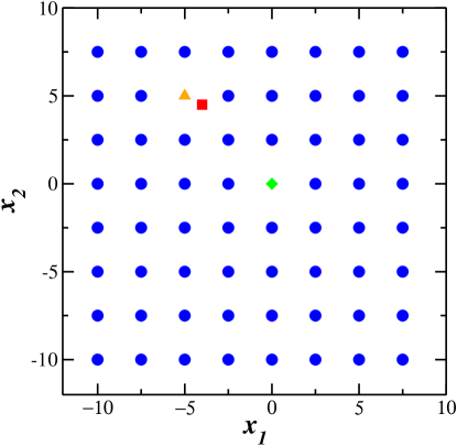
Figure 1: The $64=2^{3\times 2}$ vectors $\mathbf{x}(\mathbf{q})$ used to represent possible solutions, with $R=3$ e $N=2$. The green diamond corresponds with the initial guess $\mathbf{x}_{0}$, the red square is the exact solution, and the orange triangle is the vector $\mathbf{x}(\mathbf{q}^{*})$ that minimizes the functional $f(\mathbf{x})$ restricted to the possible 64 QUBO vectors, with $f\left(\mathbf{x(\mathbf{q}^{*})}\right)=1$ and $\mathbf{q}^{*}=(0,1,0,1,1,0)$. In the figure, $x_{1}$ and $x_{2}$ express the first and second coordinates of the vectors.

$$f(\mathbf{q})=||\mathbf{A}_{\mathbf{q}}\cdot\mathbf{q}-\mathbf{b}_{\mathbf{q}}||^{2},$$ (7)

where $\mathbf{A}_{\mathbf{q}}=\mathbf{A}\otimes(2^{0},2^{-1},2^{-2},\cdots,2^{1-R})$, with $\otimes$ the matrix kronecker product and $\mathbf{b}_{\mathbf{q}}=(\mathbf{b}+L\mathbf{A}\cdot\mathbf{I}-\mathbf{A}\cdot\mathbf{x}_{0})/L$

In our particular case we have

$$\mathbf{A}_{\mathbf{q}}=\begin{pmatrix}1&0.5&0.25&2&1&0.5\\ 3&1.5&0.75&4&2&1\ \end{pmatrix},\,\,\mathrm{and}\,\,\mathbf{b}_{\mathbf{q}}=\begin{pmatrix}3.5\\ 7.6\end{pmatrix}$$ (8)

To construct the QUBO matrix used in eq. (1), we expand $f(\mathbf{q})=\left[(\mathbf{A}_{\mathbf{q}}\cdot\mathbf{q}-\mathbf{b}_{\mathbf{q}})\cdot(\mathbf{A}_{\mathbf{q}}\cdot\mathbf{q}-\mathbf{b}_{\mathbf{q}})\right]$. Neglecting the constant positive term $\mathbf{b}_{\mathbf{q}}\cdot\mathbf{b}_{\mathbf{q}}$, we obtain the symmetric QUBO matrix

$$\mathbf{Q}=\mathbf{A}_{\mathbf{q}}^{T}\cdot\mathbf{A}_{\mathbf{q}}-2*\mathrm{Diag}\left(\mathbf{A}_{\mathbf{q}}^{T}\cdot\mathbf{b}_{\mathbf{q}}\right),$$ (9)

where $\mathrm{Diag}(\cdots)$ converts a $N$-vector in a diagonal $N\times N$ matrix. For our concrete case, we have:

$$\mathbf{Q}=\begin{pmatrix}-42.6&5&2.5&14&7&3.5\\ 5&-23.8&1.25&7&3.5&1.75\\ 2.5&1.25&-12.525&3.5&1.75&0.875\\ 14&7&3.5&-54.8&10&5\\ 7&3.5&1.75&10&-32.4&2.5\\ 3.5&1.75&0.875&5&2.5&-17.45\end{pmatrix}.$$

The binary vector $\mathbf{q}^{*}=(0,1,0,1,1,0)$ minimizes the functional $f(\mathbf{q})$. In figure 1, the orange point represents $x(\mathbf{q}^{*})$, and it is the closest point to the exact solution of the problem (the red end). Once the vector $\mathbf{x}(\mathbf{q}^{*})$ is found using a QUBO-solver, we repeat the process to find a better solution (closest to the exact solution $\mathbf{x}^{*}$) redefining $\mathbf{x}_{0}\to\mathbf{x}(\mathbf{q}^{*})$  and a new $L^{*}$, smaller than the previous $L$, in such way that the new $N$-cube contains a solution closer to the exact one.

For our concrete example ($RN=6$), verifying all the configurations and determining the best solution is easy. However, when $N$ is big, this procedure is not possible because the space of configurations is too large. A new search algorithm, different than the brute force approach, is necessary. There are different possibilities, such as simulated annealing algorithm Alkhamis1998 , Metaheuristic algorithms Dunning2018 , particular purpose quantum hardware such as quantum annealing machines Hauke2020 ; Souza2021 and classical Ising machines Mohseni2022 . Hybrid procedures using quantum and classical computation are still possible Booth2020 .

Other algorithms to tackle QUBO problems are mentioned in the review Kochenberger2014 . Once a QUBO-solver is chosen, we can use the iterative process to find the solution of the linear equations system. The Pseudo-code is presented in algorithm 1

  Function Solve($\mathbf{A}$, $\mathbf{b}$, $\mathbf{x}_{0}$, $L$, $N_{\mathrm{Iter}}$, $R$, c):

          $\mathbf{I}\leftarrow(1,1,1,\cdots,1)$

          $\mathbf{A}_{\mathbf{q}}\leftarrow\mathbf{A}\otimes(2^{0},2^{-1},2^{-2},\cdots,2^{1-R})$

          $\mathbf{Q}_{0}\leftarrow\mathbf{A}_{\mathbf{q}}^{T}\cdot\mathbf{A}_{\mathbf{q}}$

          for $k\leftarrow 1$ to $N_{\mathrm{Iter}}$ do:

                 $\mathbf{b}_{\mathbf{q}}\leftarrow(\mathbf{b}+L\mathbf{A}\cdot\mathbf{I}-\mathbf{A}\cdot\mathbf{x}_{0})/L$

                 $\mathbf{Q}\leftarrow\mathbf{Q}_{0}-2*\mathrm{Diag}\left(\mathbf{A}_{\mathbf{q}}^{T}\cdot\mathbf{b}_{\mathbf{q}}\right)$

                 Apply QUBO-solver($\mathbf{Q}$)

                 obtain $\mathbf{q}$

                 for $i\leftarrow 1$ to $N$ do:

                         $\hat{x}_{i}\leftarrow\sum_{r=0}^{R-1}q_{i}^{(r)}2^{-r}$

                 end for

                 $\hat{\mathbf{x}}\leftarrow(\hat{x}_{1},\cdots,\hat{x}_{N})$

                 $\mathbf{x}_{0}\leftarrow\mathbf{x}_{0}+L\left(\hat{\mathbf{x}}-\mathbf{I}\right)$

                 $L\leftarrow L/c$

          end for

          $\mathbf{x}^{*}\leftarrow\mathbf{x}_{0}$

  end Function

Algorithm 1 Preparation of the QUBO problem to solve a linear system of equations $\mathbf{A}\cdot\mathbf{x}=\mathbf{b}$, where $\mathbf{x}_{0}$ is the initial guess, $N_{\mathrm{Iter}}$ is the number of iterations used in the algorithm, $R$ is the bit approximation used for $\hat{x}_{i}$ and $c$ is a constant with $1<c$

Once obtained $\mathbf{x}^{*}$, we can determine $f(\mathbf{x}^{*})$ to see how much the vector $\mathbf{x}^{*}$ is close to the exact solution.

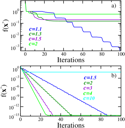
Figure 2: Iterative QUBO resolution of the linear system (5). For each iteration, a vector $\mathbf{x}^{*}$ is obtained, and we plot $f(\mathbf{x}^{*})$.We use $R=2$ in (a) and $R=3$ (b). In both cases, the convergence is faster for higher values of c. However, if c is too high, the convergence is lost.

In figure 2, we study the convergence of the iterative algorithm for different values of $R$ and $c$. As the dimension of the QUBO matrix is small, we guarantee that in each step, the QUBO solution $\mathbf{q}^{*}$ is the one that minimizes $f(\mathbf{q})$ between all the possible $\mathbf{q}$’s. Notice the particular dependence of the parameters $R$ and $c$. For sufficiently small $c$, we always have convergence with many iterations. This parameter determines the size of the search area in each iteration; for small c, we have a large area, which results in a slow convergence. A larger $c$ may improve convergence or may cause the exact solution to fall outside the neighborhood defined by the cube $N$, eliminating convergence.

Figure 3: Iterative QUBO resolution of a system with $N=20$. For each iteration, a vector $\mathbf{x}^{*}$ is obtained, and we plot $f(\mathbf{x}^{*})$. In the figure (a), we use $R=3$ and three different values of the constant $c$. In the figure (b), we use $R=6$. In both cases, a heuristic algorithm was used to solve the QUBO problem in each step. The chosen values of c are small, which implies a large number of iterations.

In figure 3, we solve 20 linear equations with 20 variables. The matrix $\mathbf{A}$ and the vector $\mathbf{b}$ associated with the problem were generated using random numbers between 0 and 200. Here, we use the open-source heuristic algorithm Qbsolv in classical simulation (which uses Tabu search and classical simulated annealing). In figure 3, we see that the efficiency of the heuristic algorithm is better for the case $R=3$ than for $R=6$. The $R=6$ case has a higher concentration of configurations around the solution. However, the associated QUBO problem is bigger than the $R=3$ case, and the QUBO-solver can not find optimal solutions for iterations. We note that the algorithm’s efficiency depends on the particular problem to solve when we use the heuristic. In the specific case shown in the figure, we have a good performance, but for other matrices with the same dimension and parameters, we could have less efficiency in finding the solution. We have no guarantee that the heuristic algorithm always determines the minimal solution. Sometimes, the heuristic algorithm can determine wrong solutions, influencing the convergence in the total iterative process.

The convergence of the iterative process also depends on the initial guess $\mathbf{x}_{0}$. This property resembles the gradient descent algorithm used in minimization problems, where the convergence rate can intensely depend on the initial guess. This drawback is solved in the descent methods, considering the geometry of the problem and reformulating it in a more powerful conjugate gradient descent method. Next, we show that the geometry associated with the system of linear equations can improve the convergence and break a sizeable original system into smaller ones that could be solved separately.

III The rhombus geometry applied to the problem $\mathbf{A}\cdot\mathbf{x}=\mathbf{b}$

III.1 The geometry of the problem $\mathbf{A}\cdot\mathbf{x}=\mathbf{b}$

The entire discrete set of possible configurations defines the QUBO. Generally, there is little structure in this set. However, since the problem is written in the language of vector space, there is a robust mathematical structure that we can use to improve the performance of existing algorithms. It is not difficult to see that the subset of $\mathbb{R}^{N}$ where $f(\mathbf{x})$ (given by eq (6) with $\mathbf{A}$ invertible) is constant corresponds to ellipsoidal hyper-surfaces of dimension $N-1$. For $N=2$ see figure 4

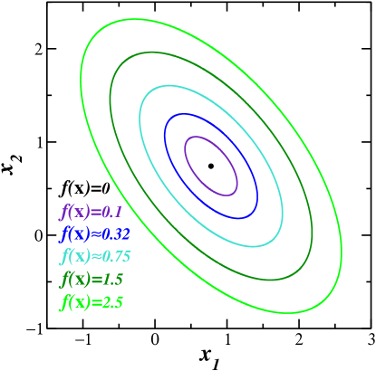
Figure 4: Concentric ellipsoidal geometry in the inversion problem (6) for a particular case when $N=2$. $\mathbf{A}$ is invertible and the ellipsoids corresponds to the regions in $\mathbb{R}^{N}$ where $f(\mathbf{x})$ is constant. All the ellipsoids are concentric and contractible to the point $\mathbf{x}^{*}$ (black point), which is the unique point that satisfies $\mathbf{A}\cdot\mathbf{x}^{*}=\mathbf{b}$. In the figure, $x_{1}$ and $x_{2}$ express the first and second coordinates of the vectors.

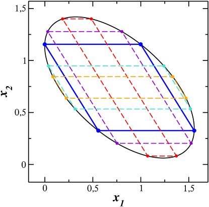
Figure 5: Family of parallelograms contained in a representative ellipse of the figure 4. The parallelograms have different side lengths and identical interior angles. In the figure, we highlight the parallelogram with equal-length sides (rhombus) in blue, which would be the base of our method to solve the problem $\mathbf{A}\cdot\mathbf{x}=\mathbf{b}$. In the figure, $x_{1}$ and $x_{2}$ express the first and second coordinates of the vectors.

All the ellipses in figure 4 are concentric and similar. Therefore, we can take a unique representative. Each ellipse contains a family of parallelograms with different sizes and interior angles; see figure 5. In figure 1, the problem is formulated in a square lattice geometry. However, nothing prevents us from using another geometry, especially one adapted to the problem. We can choose a lattice with the parallelogram geometry. In particular, we choose the parallelogram with equal-length sides (rhombus). In figure 6, we show how possible configurations are chosen using the rhombus geometry.

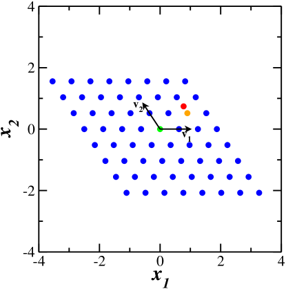
Figure 6: Space configurations of the QUBO problem in the rhombus geometry (The green point corresponds with the initial guess $\mathbf{x}_{0}$, the red point is the exact solution, and the orange circle is the point $\mathbf{x}(\mathbf{q}^{*})$ that minimizes the functional $f(\mathbf{x})$ between the lattice blue points). The unitary vectors $\mathbf{v}_{1}$ and $\mathbf{v}_{2}$ are the lattice vectors that define the rhombus geometry. In the figure, $x_{1}$ and $x_{2}$ express the first and second coordinates of the vectors.

The choice of this geometry brings advantages in the total algorithm efficiency since we need only a few quantities of iterations with the rhombus geometry to obtain convergence to the solution. In order to understand this, consider the optimal configuration $\mathbf{x}^{*}$ (big red point in figure 7), an arbitrary ellipsoid of figure 4 centered in $\mathbf{x}^{*}$ and $2^{N}$ points $\mathbf{x}_{k}$’s defining the rhombus geometry (red ellipse and the four tiny red points in figure 7). Consider another arbitrary point $\mathbf{x}_{0}$ (big blue point in figure 7), which defines a new set of similar rhombus vectors $\mathbf{y}_{k}$’s (four tiny cyan and blue points in figure 7); for $N=2$, these rhombus vectors define the dashed rhombus of figure 7 which is divided in $4$ sub-rhombus ($2^{N}$ in the arbitrary case). Suppose that $\mathbf{x}^{*}$ is inside of this rhombus and, therefore, also is inside of a particular sub-rhombus associated with the point $\mathbf{y}_{l}$ (tiny cyan point in the left inferior corner of figure 7), then, between the four $\mathbf{y}_{k}$’s the evaluated function $f(\mathbf{y}_{l})$ reach the minimal value (in the figure 7, the tiny cyan point in the left inferior corner is contained in the smaller cyan ellipse), see figure 7. We call this property the rhombus convergence, which is proved in the appendix. The property improves the convergence since the point associated with the QUBO solution $\mathbf{x}^{*}$ in each iteration is also contained in the next constructed tiny rhombus.

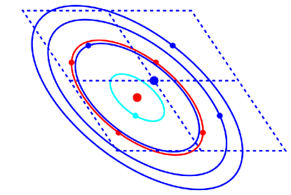
Figure 7: The figure shows the rhombus defined by the geometry of the problem; the tiny cyan and blue points are the QUBO configurations $\mathbf{y}_{k}$ around the big blue point $\mathbf{x}_{0}$ in the center of the rhombus. There are $2^{N}$ points (in the figure, $N=2$), and with each point, an associated sub-rhombus. The big red point $\mathbf{x}^{*}$ satisfy $f(\mathbf{x}^{*})=0$ and $\mathbf{x}^{*}=\mathbf{x}_{0}+\mathbf{t}$, with $\mathbf{t}$ the difference vector. In the figure, the tiny red vectors satisfy $\mathbf{x}_{k}=\mathbf{y}_{k}+\mathbf{t}$ and $f(\mathbf{x}_{k})=C$ for all $k$. The cyan and blue ellipses express the different values of $f(\mathbf{y}_{k})$. The big red point $\mathbf{x}^{*}$ is contained in the left-inferior sub-rhombus, and the associated cyan point $\mathbf{y}_{l}$ in their center satisfy $f(\mathbf{y}_{l})<f(\mathbf{y}_{k})$ for all $k\neq l$.

We emphasize that the square geometry used in previous works only coincides with the matrix inversion geometry when the matrix $\mathbf{A}$ is diagonal. For non-diagonal matrices in the square geometry, the closest point (in the conventional distance) to the exact solution $\mathbf{x}^{*}$ is not necessarily the point with the most negligible value of $f(\mathbf{x})$ between the finite QUBO vectors. In other words, the exact solution $\mathbf{x}^{*}$ would lay outside the region containing the QUBO configurations, breaking the convergence. We can avoid the lack of convergence by diminishing the parameter $c$ or increasing the number $R$ in the algorithm but with the consequence of increasing the number of iterations.

III.2 $\mathbf{H}$-orthogonality

The ellipsoid form in the matrix inversion problem is given by the symmetric matrix $\mathbf{H}=\mathbf{A}^{T}\mathbf{A}$, this is clear when we define the new function $f_{0}(\mathbf{x})=\|\mathbf{A}\cdot\mathbf{x}\|$, which define the same set of similar ellipsoids but centered in the zero vector. Particularly, the matrix $\mathbf{H}$ define a notion of orthogonality called in the review Shewchuk1994 as $\mathbf{H}$-orthogonality, where two vectors $\mathbf{v}_{1}$ and $\mathbf{v}_{2}$ in $\mathbb{R}^{N}$ are $\mathbf{H}$-orthogonal if they satisfy

$$\langle\mathbf{v}_{1},\mathbf{v}_{2}\rangle_{\mathbf{H}}\equiv\mathbf{v}_{1}\cdot\left(\mathbf{A}^{T}\mathbf{A}\cdot\mathbf{v}_{2}\right)=0.$$ (10)

Given the $N$’s canonical vectors $\mathbf{u}_{k}$, with the $k$-th coordinate equal to one and all others equal to zero. We can construct from them $N$ $\mathbf{H}$-orthogonal vectors $\mathbf{v}_{k}$ associated with each $\mathbf{u}_{k}$ using a generalized Gram-Schmidt $\mathbf{H}$-orthogonalization. The method selects the first vector as $\mathbf{v}_{1}=\mathbf{u}_{1}$. The vector $\mathbf{v}_{m}$ is constructed as

$$\mathbf{v}_{m}=\mathbf{u}_{m}+\sum_{k=1}^{m-1}\beta_{mk}\mathbf{v}_{k}.$$ (11)

The coefficients $\beta_{mk}$ are determined using the $\mathbf{H}$-orthogonality property $\langle\mathbf{v}_{m},\mathbf{v}_{k}\rangle_{\mathbf{H}}=0$. Explicitly

$$\beta_{mk}=-\frac{\langle\mathbf{v}_{k},\mathbf{u}_{m}\rangle_{\mathbf{H}}}{\langle\mathbf{v}_{k},\mathbf{v}_{k}\rangle_{\mathbf{H}}}.$$ (12)

  Function Ortho($\mathbf{A}$,$N$):

          $\mathbf{H}\leftarrow\mathbf{A}^{T}\cdot\mathbf{A}$

          for $k\leftarrow 1$ to $N$ do:

                 If $k=1$ then

                         $\mathbf{v}_{k}\leftarrow\mathbf{u}_{k}$

                 Else

                         $\mathbf{v}_{k}\leftarrow\mathbf{u}_{k}$

                         for $m\leftarrow 1$ to $k-1$ do:

                                $\mathbf{v}_{k}\leftarrow\mathbf{v}_{k}+\beta_{km}\mathbf{v}_{m}$

                         end for

                 $\mathbf{v}_{k}\leftarrow\mathbf{v}_{k}/\left(\mathbf{v}_{k}\cdot\mathbf{v}_{k}\right)^{1/2}$

                 end If

                 $\mathbf{O}_{k}\leftarrow\mathbf{H}\cdot\mathbf{v}_{k}$

                 $C_{k}\leftarrow\mathbf{v}_{k}\cdot\mathbf{O}_{k}$

                 for $r\leftarrow 1$ to $k+1$ do:

                         If $k<N$ then

                                $\beta_{(k+1)r}=-\mathbf{O}_{r}\cdot\mathbf{u}_{k+1}/C_{r}$

                         end If

                 end for

          end for

  end Function

Algorithm 2 Gram-Schmidt procedure for the calculus of the $N$’s $\mathbf{H}$-orthogonal vectors $(\mathbf{v}_{1},\cdots,\mathbf{v}_{N})$

The calculated non-orthogonal unitary vectors (in the standard scalar product) $\mathbf{v}_{k}$ define the rhombus geometry previously described.

III.3 The modified search region

Considering the intrinsic rhombus geometry, the iterative algorithm converges exponentially fast in the number of iterations and is sufficient to use $R=1$. The QUBO configurations in (4) around a determinate guess can be rewritten as

$$\mathbf{x}=\mathbf{x}_{0}+L\sum_{i=1}^{N}\left(\hat{x}_{i}-1\right)\mathbf{u}_{i}$$ (13)

with $\mathbf{u}_{i}$ the canonical base. Therefore, we modified the algorithm 1 changing $\mathbf{u}_{i}\to\mathbf{v}_{i}$, $\hat{x}_{i}\to q_{i}$ and $\mathbf{I}\to\mathbf{I}/2$. The last modification localizes the initial guess (or the previously founded QUBO solution) in the center of the rhombus. We have $q_{i}\in\{0,1\}$. The $2^{N}$ QUBO configurations are the vertices of a $N$-rhombus and are associated with all the possible binary vectors $\mathbf{q}=(q_{1},\cdots,q_{N})$. We can substitute this modifications in the function $f(\mathbf{x})$ and calculate $\mathbf{A}_{\mathbf{q}}$ and $\mathbf{b}_{\mathbf{q}}$. Considering the vectors $\mathbf{v}_{i}$ as the $i$th row of a matrix $\mathbf{V}$ (this is $V_{ij}=\mathbf{v}_{i}\cdot\mathbf{u}_{j}$) is not difficult to see that

$$\mathbf{A}_{\mathbf{q}}=\mathbf{A}\mathbf{V}^{T}$$ (14)

and

$$\mathbf{b}_{\mathbf{q}}=(\mathbf{b}+\frac{L}{2}\mathbf{A}_{\mathbf{q}}\cdot\mathbf{I}-\mathbf{A}\cdot\mathbf{x}_{0})/L.$$ (15)

From equation (9) and the $\mathbf{H}$-orthogonality of the vectors $\mathbf{v}_{i}$ (matrix rows of $\mathbf{V}$), it is possible to see that the QUBO matrix $\mathbf{Q}$ constructed from (14) is always diagonal. The QUBO solution is trivial (this means that there are no necessary heuristic algorithms or quantum computers to solve the QUBO problem). We show the modified iterative process in the algorithm 3.

  Function Solve($\mathbf{A}$, $\mathbf{b}$, $\mathbf{x}_{0}$, $L$, $N_{\mathrm{Iter}}$, $c$):

          from Ortho($\mathbf{A}$,$N$) obtain

                  $\mathbf{V}\leftarrow(\mathbf{v}_{1},\mathbf{v}_{2}\cdots,\mathbf{v}_{N})^{T}$

                  $\mathbf{C}\leftarrow(C_{1},C_{2},\cdots,C_{N})$

          $\mathbf{I}\leftarrow(1,1,1,\cdots,1)$

          $\mathbf{A}_{\mathbf{q}}\leftarrow\mathbf{A}\mathbf{V}^{T}$

          for $k\leftarrow 1$ to $N_{\mathrm{Iter}}$ do:

                 $\mathbf{b}_{\mathbf{q}}\leftarrow(\mathbf{b}+\frac{L}{2}\mathbf{A}_{\mathbf{q}}\cdot\mathbf{I}-\mathbf{A}\cdot\mathbf{x}_{0})/L$

                 $\mathbf{Q}\leftarrow\mathbf{C}-2*\mathbf{A}_{\mathbf{q}}^{T}\cdot\mathbf{b}_{\mathbf{q}}$

                 for $i\leftarrow 1$ to $N$ do:

                         If $Q_{i}<0$ then

                                $q_{i}\leftarrow 1$

                         Else

                                $q_{i}\leftarrow 0$

                         end If

                 end for

                 $\hat{\mathbf{x}}\leftarrow(q_{1},q_{2},\cdots,q_{N})$

                 $\mathbf{x}_{0}\leftarrow\mathbf{x}_{0}+L\mathbf{V}^{T}\cdot\left(\hat{\mathbf{x}}-\mathbf{I}/2\right)$

                 $L\leftarrow L/c$

          end for

          $\mathbf{x}^{*}\leftarrow\mathbf{x}_{0}$

  end Function

Algorithm 3 Modified iterative algorithm using the rhombus geometry. The $C_{k}$ numbers are calculated in algorithm 2.

The algorithm works whenever the rhombus that contains the QUBO configurations also includes the exact solution $\mathbf{x}^{*}$. This is guaranteed when $L$ is sufficiently large (in particular when $L>L_{0}$, where $L_{0}$ is the “critical” value parameter to obtain convergence). In figure 8, we show the algorithm performance for a particular dense matrix with dimension $5000\times 5000$. The initial guess is the $N$-dimensional zero vector ($N=5000$). Notice the dependence with the parameter value $c$; the critical value is $c=2$, and there is no convergence for $c>2$. To compare with the original algorithm, we study the case with $N=500$, corresponding to a QUBO problem with 1500 variables ($N=500$ and $R=3$). Figure 9 compares the two different approaches. The original algorithm in Figure b) has poor efficiency compared to the modified algorithm shown in Figure a).

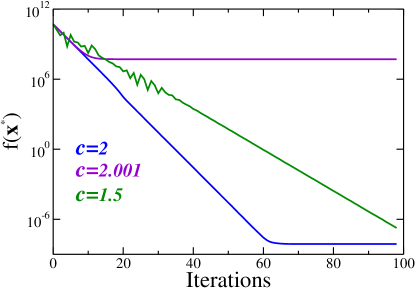
Figure 8: Iterative QUBO modified algorithm applied to a linear system with 5000 variables and 5000 equations. Note the fast convergence rate to the exact solution in a few iterations (cases $c=2$ and $c=1.5$). All the $2.5\times 10^{7}$ matrix coefficients of $\mathbf{A}$ and the 5000 vector coefficient of $\mathbf{b}$ were generated using random numbers between 0 and 200. In the modified algorithm we use $L=61000$ and initial guess $\mathbf{x}_{0}=(0,0,\cdots,0)$. Considering $\mathbf{x}_{\mathrm{Inv}}=\mathbf{A}^{-1}\cdot\mathbf{b}$ as the solution obtained by classical inversion algorithms, we have $f(\mathbf{x}_{\mathrm{Inv}})\approx 7.07\times 10^{-7}$. We obtain $f(\mathbf{x}^{*})\approx 7.08\times 10^{-9}$ with our modified QUBO algorithm. For $c>2$, the convergence is drastically destroyed.

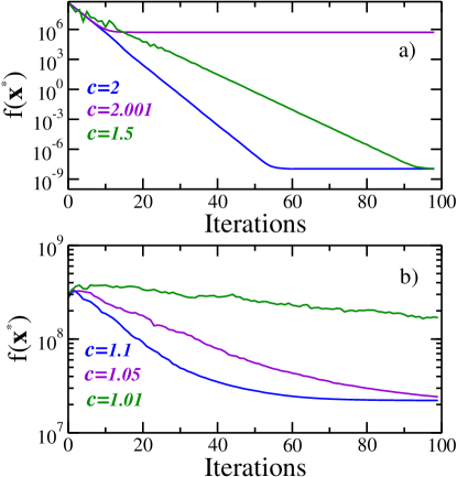
Figure 9: Comparison between the iterative algorithms 3 (Figure a)) and algorithm 1 Figure b) for a matrix with $N=500$ and the same initial $L$. The modified algorithm performs substantially better than the original (see Figure a)). The function $f(\mathbf{x}^{*})$ for the vector $\mathbf{x}^{*}$ obtained in the final iteration is very close to zero). Algorithm 1 (figure b)) using Qbsolv as QUBO-solver in the standard configuration does not show convergence. In the two cases, the initial guess $\mathbf{x}_{0}$ is the zero vector.

In the last section of this work, we show that a partial knowledge of the conjugated vectors $\mathbf{v}_{i}$ also simplifies the original QUBO problem enormously.

IV Solving Large systems of equations using binary optimization

IV.1 Decomposing QUBO matrices in small sub-problems.

In the previous section, we show that the knowledge of the conjugated vectors that generate the rhombus geometry simplifies the QUBO resolution and improves the convergence rate to the exact solution. However, the calculus of these vectors in our algorithm 2 has approximately $O(N^{3})$ steps. A faster algorithm would be desirable.

Another interesting possibility is to use the notion of $H$-orthogonality to construct a different set of $N$ vectors $\mathbf{v}_{i}$ grouped in $m$ different subsets in such a way that vectors in different subsets be $H$-orthogonal. In this last section, we show that such construction decomposes the original QUBO matrix in a Block diagonal form, and we can use a modified version of our algorithm 3. We can tackle each block independently for some QUBO-solver, and after joining the independent results, we obtain the total solution. There are a total of $2^{N-1}$ possible decompositions for each possible numerical composition of the number $N$. A composition of $N$ is $(a_{1},a_{2},\cdots,a_{m})$ where $N=a_{1}+a_{2}+\cdots+a_{m}$ and each $a_{k}\in\mathbb{N}$.

Techniques of decomposition in sub-problems are standard in the search process in some QUBO-solvers. We mention the QUBO-solver Qbsolv, a heuristic hybrid algorithm that decomposes the original problem into many QUBO sub-problems that can be approached using classical Ising or Quantum QUBO-solvers. The solution of each sub-problem is projected in the actual space to infer better initial guesses in the classical heuristic algorithm (Tabu search) and potentiate the search process; see reference Booth2017 for details. Our algorithm decomposes the original QUBO problem associated with $\mathbf{A}\cdot\mathbf{x}=\mathbf{b}$ in many independent QUBO sub-problems. We obtain the optimal solution directly from the particular sub-solutions of each QUBO sub-problem.

To see how the method works, we use the generalized Gram-Schmidt orthogonalization only between different groups of vectors. First call

$$\mathbf{v}_{i}^{(1)}=\mathbf{u}_{i},\,\,\,\,\,\,\,\,\mathrm{If}\,\,\,\,\,\,\,\,i\in\{1,\cdots,a_{1}\}.$$ (16)

For the other vectors, we use

$$\mathbf{v}_{j}^{(1)}=\mathbf{u}_{j}+\sum_{k=1}^{a_{1}}\beta_{jk}\mathbf{v}_{k}^{(1)},\,\,\,\,\,\,\,\,\mathrm{If}\,\,\,\,\,\,\,\,j\in\{a_{1}+1,\cdots,N\}.$$ (17)

We also demand that the first group of $a_{1}$ vectors be $H$-orthogonal to the second group of $N-a_{1}$ vectors, this is for $j\in\{a_{1}+1,\cdots,N\}$:

$$\langle\mathbf{v}_{k}^{(1)},\mathbf{v}_{j}^{(1)}\rangle_{\mathbf{H}}=0,\,\,\,\mathrm{If}\,\,\,\, k\in\{1,\cdots,a_{1}\}\,\,\,\mathrm{and}\,\,\,$$

$$j\in\{a_{1}+1,\cdots,N\}.$$ (18)

This last condition determines all the coefficients $\beta_{jk}$ for each $j$, solving a linear system of dimension $a_{1}\times a_{1}$. For fixed $j$ and defining $\bm{\mathbf{\beta}}_{j}=(\beta_{j1},\beta_{j2},\cdots,\beta_{ja_{1}})$, it is not difficult to see that the linear system to solve is

$$\bm{\mathbf{\beta}}_{j}=-\mathbf{H}_{a_{1}}^{-1}\cdot\mathbf{h}_{j},$$ (19)

where $\mathbf{H}_{a_{1}}$ is the sub-matrix of $\mathbf{H}$ corresponding with their first $a_{1}\times a_{1}$ block sub-matrix, and $\mathbf{h}_{j}$ are the first $a_{1}$’s coefficients of the $j$-column of $\mathbf{H}$. With the coefficients $\bm{\beta}_{j}$ we can calculate $\mathbf{v}_{j}^{(1)}$ and normalize it. Grouping all these vectors as the rows of the matrix $\mathbf{V}_{(1)}$, it is possible to verify that

$$\mathbf{V}_{(1)}\cdot\mathbf{H}\cdot\mathbf{V}_{(1)}^{T}=\mathbf{H}_{a_{1}}\oplus\mathbf{H}^{(1)},$$ (20)

where $\mathbf{H}^{(1)}$ is a $(N-a_{1})\times(N-a_{1})$ matrix. We can put $\mathbf{H}^{(1)}$ in a two-block diagonal form by the same process, where one block has dimension $a_{2}\times a_{2}$ and the second block has dimension $(N-a_{1}-a_{2})\times(N-a_{1}-a_{2})$. Briefly

$$\mathbf{v}_{i}^{(2)}=\mathbf{u}_{i},\,\,\,\,\,\,\,\,\mathrm{If}\,\,\,\,\,\,\,\,i\in\{0,1,\cdots,a_{1}+a_{2}\},$$ (21)

and

$$\mathbf{v}_{j}^{(2)}=\mathbf{v}_{j}^{(1)}+\sum_{k=a_{1}+1}^{a_{1}+a_{2}}\beta_{jk}^{(1)}\mathbf{v}_{k}^{(2)},\,\,\,\,\,\mathrm{If}\,\,\,\,\,j\in\{a_{1}+a_{2}+1,\cdots,N\}.$$ (22)

To determine the new set of $\beta$ coefficients, we use

$$\bm{\mathbf{\beta}}_{j}^{(1)}=-{\mathbf{H}_{a_{2}}^{-1}}\cdot\mathbf{h}_{j}^{(1)},$$ (23)

where $\bm{\mathbf{\beta}}_{j}^{(1)}=(\beta_{j,a_{1}+1}^{(1)},\beta_{j,a_{1}+2}^{(1)},\cdots,\beta_{j,a_{1}+a_{2}}^{(1)})$, $\mathbf{H}_{a_{2}}$ is the first $a_{2}\times a_{2}$ block diagonal matrix of $\mathbf{H}^{(1)}$ and $\mathbf{h}_{j}^{(1)}$ are the first $a_{2}$’s coefficients of the $j$-column of $\mathbf{H}^{(1)}$.  Repeating the previous procedure, we obtain a new matrix $\mathbf{V}_{(2)}$, which has the property

$$\mathbf{V}_{(2)}\cdot\left(\mathbf{V}_{(1)}\cdot\mathbf{H}\cdot\mathbf{V}_{(1)}^{T}\right)\cdot\mathbf{V}_{(2)}^{T}=\mathbf{H}_{a_{1}}\oplus\mathbf{H}_{a_{2}}\oplus\mathbf{H}^{(2)}.$$ (24)

Repeating the same process another $(m-3)$ times and defining

$$\mathbf{V}\equiv\mathbf{V}_{m-1}\cdot\mathbf{V}_{m-2}\cdots\mathbf{V}_{2}\cdot\mathbf{V}_{1}$$ (25)

and $\mathbf{H}^{(m-1)}\equiv\mathbf{H}_{a_{m}}$, we obtain

$$\mathbf{V}\cdot\mathbf{H}\cdot\mathbf{V}^{T}=\mathbf{H}_{a_{1}}\oplus\mathbf{H}_{a_{2}}\oplus\cdots\oplus\mathbf{H}_{a_{m}}$$ (26)

We use the notation with $\mathbf{H}_{a_{k}}$ to reinforce that this is a $a_{k}\times a_{k}$ matrix. For concrete problems is better to use $\mathbf{H}_{a_{k}}\equiv\mathbf{H}_{k}$. We implement this procedure in the pseudo-code 4.

  Function OrthoBlock($\mathbf{A}$,$N$,$\{a_{1},a_{2},\cdots,a_{m}\}$):

          $\mathbf{H}\leftarrow\mathbf{A}^{T}\cdot\mathbf{A}$

          for $k\leftarrow 1$ to $m-1$ do:

                 If $k=1$ then

                         $\mathbf{V}\leftarrow\mathrm{Diag}\left(\mathbf{I}\right)$

                 end If

                 $\mathbf{H}_{I}\leftarrow\mathbf{H}_{a_{k}}^{-1}$

                 for $r\leftarrow 1$ to $N$ do:

                         If $r\leq a_{1}+a_{2}+\cdots a_{k}$ then

                                $\mathbf{v}_{r}\leftarrow\mathbf{u}_{r}$

                         Else

                                $\bm{\beta_{r}}\leftarrow-\mathbf{H}_{I}\cdot\mathbf{H}[a_{k-1}::a_{k},r]$

                                $\mathbf{v}_{r}\leftarrow\mathbf{u}_{r}+\sum_{l=1}^{a_{k}}\beta_{rl}\mathbf{v}_{a_{1}+\cdots+a_{k-1}+l}$

                                $\mathbf{v}_{r}\leftarrow\mathbf{v}_{r}/\left(\mathbf{v}_{r}\cdot\mathbf{v}_{r}\right)^{1/2}$

                         end If

                 end for

                 $\mathbf{V}^{*}\leftarrow(\mathbf{v}_{1},\mathbf{v}_{2}\cdots,\mathbf{v}_{N})^{T}$

                 $\mathbf{H}\leftarrow\mathbf{V}^{*}\cdot\left(\mathbf{H}\cdot{\mathbf{V}^{*}}^{T}\right)$

                 $\mathbf{V}\leftarrow\mathbf{V}^{*}\cdot\mathbf{V}$

          end for

  end Function

Algorithm 4 Block diagonal transformation of the matrix $\mathbf{H}$ associated with the composition $(a_{1}.a_{2},\cdots,a_{m})$ from the partial $\mathbf{H}$-orthogonalization process described in the construction of equation (26). In the pseudo-code the notation is $\bm{\beta}_{r}=(\beta_{r1},\beta_{r2},\cdots,\beta_{ra_{k}})$ and $\mathbf{H}[a_{k-1}::a_{k},r]$ correspond with the $r$ sub-column of $\mathbf{H}$ beginning in the row component $a_{1}+\cdots+a_{k-1}+1$ and finishing in $a_{1}+\cdots+a_{k-1}+a_{k}$.

IV.2 Implementation of the algorithm

  Function Solve($\mathbf{A}$, $\mathbf{b}$, $\mathbf{x}_{0}$, $L$, $N_{\mathrm{Iter}},R,c$):

          from OrthoBlock($\mathbf{A}$,$N$,$\{a_{1},a_{2},\cdots,a_{m}\}$) obtain

                  $\mathbf{V}\leftarrow(\mathbf{v}_{1},\mathbf{v}_{2}\cdots,\mathbf{v}_{N})^{T}$

          $\mathbf{I}\leftarrow(1,1,1,\cdots,1)$

          $\mathbf{A}_{\mathbf{V}}\leftarrow\mathbf{A}\mathbf{V}^{T}$

          $\mathbf{H}_{\mathbf{V}}\leftarrow\mathbf{V}\mathbf{A}^{T}\mathbf{A}\mathbf{V}^{T}=\mathbf{H}_{1}\oplus\mathbf{H}_{2}\oplus\cdots\oplus\mathbf{H}_{m}$

          $\mathbf{A}_{\mathbf{q}}\leftarrow\mathbf{A}_{\mathbf{V}}\otimes(2^{0},2^{-1},2^{-2},\cdots,2^{1-R})$

          for $j\leftarrow 1$ to $m$ do:

                 $\mathbf{H}_{\mathbf{q}}^{(j)}\leftarrow\mathbf{H}_{j}\otimes(2^{0},2^{-1},2^{-2},\cdots,2^{1-R})$

                 $\mathbb{I}_{\mathbf{q}}^{(j)}\leftarrow\mathbb{I}_{a_{j}\times a_{j}}\otimes(2^{0},2^{-1},2^{-2},\cdots,2^{1-R})$

                 $\mathbf{Q}_{0}^{(j)}\leftarrow({\mathbb{I}_{\mathbf{q}}^{(j)}})^{T}\mathbf{H}_{\mathbf{q}}^{(j)}$

          end for

          for $k\leftarrow 1$ to $N_{\mathrm{Iter}}$ do:

                 $\mathbf{b}_{\mathbf{q}}\leftarrow(\mathbf{b}+\frac{L}{2}\mathbf{A}_{\mathbf{V}}\cdot\mathbf{I}-\mathbf{A}\cdot\mathbf{x}_{0})/L$

                 for $i\leftarrow 1$ to $m$ do:

                         $\mathbf{Q}_{i}\leftarrow\mathbf{Q}_{0}^{(i)}-2*\mathrm{Diag}^{(a_{i})}\left(\mathbf{A}_{\mathbf{q}}^{T}\cdot\mathbf{b}_{\mathbf{q}}\right)$

                         Apply QUBO-solver($\mathbf{Q}_{i}$)

                         obtain $\mathbf{q}_{i}$

                 end for

                 $\mathbf{q}\leftarrow\mathrm{Flatten}\left(\{\mathbf{q}_{1},\mathbf{q}_{2},\cdots,\mathbf{q}_{m}\}\right)$

                 for $l\leftarrow 1$ to $N$ do:

                         $\hat{x}_{l}\leftarrow\sum_{r=0}^{R-1}q_{l}^{(r)}2^{-r}$

                 end for

                 $\hat{\mathbf{x}}\leftarrow(\hat{x}_{1},\cdots,\hat{x}_{N})$

                 $\mathbf{x}_{0}\leftarrow\mathbf{x}_{0}+L\mathbf{V}^{T}\cdot\left(\hat{\mathbf{x}}-\mathbf{I}/2\right)$

                 $L\leftarrow L/c$

          end for

          $\mathbf{x}^{*}\leftarrow\mathbf{x}_{0}$

  end Function

Algorithm 5 Modified iterative algorithm using the block diagonal decomposition of $\mathbf{H}$. Here, $\mathrm{Diag}^{(a_{i})}\left(\mathbf{A}_{\mathbf{q}}^{T}\cdot\mathbf{b}_{\mathbf{q}}\right)$ take the components of the vector $\left(\mathbf{A}_{\mathbf{q}}^{T}\cdot\mathbf{b}_{\mathbf{q}}\right)$ from the coordinate $a_{1}+\cdots+a_{i-1}+1$ until the coordinate $a_{1}+\cdots+a_{i}$ and builds a diagonal $a_{i}\times a_{i}$ matrix.

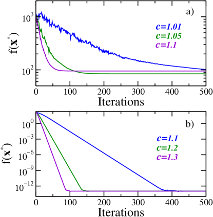
Figure 10: Iterative QUBO algorithms are applied to a linear system with 100 variables and 100 equations. All the $10^{4}$ matrix coefficients of $\mathbf{A}$ and the 100 vector coefficient of $\mathbf{b}$ were generated using random numbers between 0 and 200. We use $L=100$ and initial guess $\mathbf{x}_{0}=(0,0,\cdots,0)$. In a), we use the square geometry and Qbsolv software as the QUBO-solver. In the figure b), we decompose the original matrix in 10 sub-problems with dimension $10\times 10$. We only obtain an exact convergence to the solution using the block decomposition shown in the algorithm 5.

The procedure that decomposes and solves a QUBO problem is shown in algorithm 5. In each iterative step, a heuristic QUBO-solver is used. In figure 10, we offer the resolution of a matrix with size $100\times 100$ without the decomposition (figure 10a) and using the block decomposition (figure 10b). In figure 10a, we use the square geometry and the software Qbsolv Booth2017 as the QUBO-solver. In this case, we have obtained poor convergence for all values of $c$ tested. When the block decomposition is used, the convergence rate is fast, even in $c=1.1$; see figure 10b.

If the matrix $\mathbf{A}$ is large and has a decomposition with blocks of dimension bigger than 50, the QUBO sub-problem is still too tricky for classical algorithms. New QUBO-solvers, such as quantum annealers, can improve the general algorithm efficiency in this case. This question depends on each problem. However, if the QUBO-solver efficiently solves a specific problem, we can decompose larger matrices in many sub-problems where the QUBO-solver is effective. We intend to explore this delicate balance soon.

V Discussion

In this work, we propose a new method to solve a system of linear equations using binary optimizers. Our approach guarantees that the optimal configuration is the closest to the exact solution. Also, we show that a partial knowledge of the problem geometry allows the decomposition into a series of independent sub-problems that can be attained using conventional QUBO-solvers. The solution to each sub-problem is gathered, and an optimal solution can be rapidly found. Find the vectors that determine the sub-problem decomposition have a computational cost influencing the whole performance of the algorithm. Nevertheless, two factors can be essential to discover substantial improvements: better methods to find the vectors associated with the geometry and more powerful QUBO-solvers. In this respect, quantum computing and inspired quantum computation can be fundamental tools for finding better approaches that can be ensembled with the procedures presented here. We intend to explore these exciting questions in subsequent studies, and we hope that the methods present here can help to find better and more efficient procedures to solve extensive linear systems of equations.

Appendix A The sub-rhombus convergence

In section III.A, we define the sub-rhombus convergence statement: Given a rhombus geometry defined by a non-singular matrix $\mathbf{A}$ and a vector $\mathbf{b}$, for a given rhombus with center $\mathbf{x}_{0}$ and $2^{N}$ lattice vectors $\mathbf{y}_{k}$ (see figure 7), if the $\mathbf{x}^{*}$ point with $f(\mathbf{x}^{*})=0$ is inside of the rhombus and between the points $\mathbf{y}_{k}$, the point $\mathbf{y}_{1}$ satisfy $f(\mathbf{y}_{1})<f(\mathbf{y}_{k})$ for all $k\neq 1$, then the point $\mathbf{x}^{*}$ is inside of the sub-rhombus associated to $\mathbf{y}_{1}$. Where, $f(\mathbf{x})=\|\mathbf{A}\cdot\mathbf{x}-\mathbf{b}\|$ and $\mathbf{A}\cdot\mathbf{x}^{*}=\mathbf{b}$.

Consider that the point $\mathbf{x}^{*}$ belongs to the sub-rhombus defined by $\mathbf{y}_{1}$. We prove that the point $\mathbf{y}_{m}$ that minimize the functional $f(\mathbf{y}_{k})$ restricted to the QUBO vectors $\mathbf{y}_{k})$‘s satisfy $\mathbf{y}_{k}=\mathbf{y}_{1}$. As $\mathbf{x}^{*}$ belongs to the sub-rhombus defined by $\mathbf{y}_{1}$ we can write

$$\mathbf{x}^{*}=\mathbf{y}_{1}+\sum_{j=1}^{N}C_{j}\mathbf{v}_{j},\,\,\,\,\mathrm{with}\,\,|C_{j}|\leq\frac{L}{4}\,\,\forall\,\,j,$$ (27)

where $L$ is the side length of the principal rhombus shown in figure 7 and $\mathbf{v}_{j}$ is the vector that defines the rhombus geometry. All points inside of the sub-rhombus associated with $\mathbf{y}_{1}$ satisfied $|C_{j}|\leq\frac{L}{4}\,\,\forall\,\,j,$ and any point outside of this sub-rhombus breaks the inequality. The point $\mathbf{x}^{*}$ also belongs to the principal rhombus, therefore

$$\mathbf{x}^{*}=\mathbf{x}_{0}+\sum_{j=1}^{N}D_{j}\mathbf{v}_{j},\,\,\,\,\mathrm{with}\,\,|D_{j}|\leq\frac{L}{2}\,\,\forall\,\,j.$$ (28)

Consider a similar rhombus with the center in $\mathbf{x}^{*}$ and the associated rhombus points $\mathbf{x}_{k}$’s (blue tiny points in figure 7). It is clear that $\mathbf{x}^{*}-\mathbf{x}_{0}=\mathbf{x}_{k}-\mathbf{y}_{k}$, or

$$\mathbf{y}_{k}=\mathbf{x}_{k}-\sum_{j=1}^{N}D_{j}\mathbf{v}_{j}.$$ (29)

The functional $f(\mathbf{y}_{k})$ restricted to the points $\mathbf{y}_{k}$’s can be written as

$$f(\mathbf{y}_{k})=\|\mathbf{A}\cdot\left(\mathbf{x}^{*}-\mathbf{y}_{k}\right)\|^{2},$$ (30)

using eq.(28) and (29), we obtain

$$f(\mathbf{y}_{k})= \|\mathbf{A}\cdot(\sum_{j=1}^{N}D_{j}\mathbf{v}_{j})\|^{2}+\left\|\mathbf{A}\cdot(\mathbf{x}_{k}-\mathbf{x}^{*})\right\|^{2}$$

$$-2[\mathbf{A}\cdot(\sum_{j=1}^{N}D_{j}\mathbf{v}_{j})]\cdot[\mathbf{A}\cdot(\mathbf{x}_{k}-\mathbf{x}^{*})].$$ (31)

The two first terms of (A) are identical for all the possible $\mathbf{y}_{k}$ choices. Therefore, the minimal value of $f(\mathbf{y}_{m})$ is reached by the $\mathbf{x}_{m}$ that maximize

$$[\mathbf{A}\cdot(\sum_{j=1}^{N}D_{j}\mathbf{v}_{j})]\cdot[\mathbf{A}\cdot(\mathbf{x}_{m}-\mathbf{x}^{*})].$$

$\mathbf{x}_{k}$ belongs to the similar rhombus centered in $\mathbf{x}^{*}$ and is written as

$$\mathbf{x}_{k}=\mathbf{x}^{*}+\sum_{j=1}^{N}s_{j}^{(k)}\frac{L}{4}\mathbf{v}_{j},$$ (32)

with $s_{j}^{(k)}\in\{-1,1\}$ for all $j$. Using the property

$$(\mathbf{A}\cdot\mathbf{v}_{i})\cdot(\mathbf{A}\cdot\mathbf{v}_{j})=\mathbf{v}_{i}\cdot\left(\mathbf{A}^{T}\mathbf{A}\right)\cdot\mathbf{v}_{j}=h_{i}\delta_{ij},$$

we have

$$[\mathbf{A}\cdot(\sum_{j=1}^{N}D_{j}\mathbf{v}_{j})]\cdot[\mathbf{A}\cdot(\mathbf{x}_{k}-\mathbf{x}^{*})]=\sum_{j=1}^{N}s_{j}^{(k)}\frac{L}{4}h_{j}D_{j}.$$ (33)

To obtain the configuration that maximize (33) choose $s_{j}^{(m)}=\mathrm{Sign}(D_{j})$ (the $h_{i}$ numbers are always positive). Using

$$\|\mathbf{A}\cdot(\sum_{j=1}^{N}D_{j}\mathbf{v}_{j})\|^{2}=\sum_{j=1}^{N}h_{j}D_{j}^{2}$$ (34)

and

$$\left\|\mathbf{A}\cdot(\mathbf{x}_{m}-\mathbf{x}^{*})\right\|^{2}=\sum_{j=1}^{N}h_{j}\frac{L^{2}}{16}$$ (35)

we obtain

$$f(\mathbf{y}_{m})=\sum_{j=1}^{N}h_{j}\left(|D_{j}|-\frac{L}{4}\right)^{2}=\sum_{j=1}^{N}h_{j}E_{j}^{2},$$ (36)

or

$$\|\mathbf{A}\cdot\left(\mathbf{x}^{*}-\mathbf{y}_{m}\right)\|^{2}=\|\mathbf{A}\cdot(\sum_{j=1}^{N}E_{j}\mathbf{v}_{j})\|^{2}$$ (37)

implying in

$$\mathbf{x}^{*}=\mathbf{y}_{m}+\sum_{j=1}^{N}E_{j}\mathbf{v}_{j}$$ (38)

If we prove that $|E_{j}|\leq\frac{L}{4}\,\,\forall\,\,j$, then $E_{j}=C_{j}$ and $\mathbf{y}_{m}=\mathbf{y}_{1}$. From (36), we have

$$E_{j}^{2}=\left(|D_{j}|-\frac{L}{4}\right)^{2}$$ (39)

or

$$E_{j}^{2}-\frac{L^{2}}{16}=|D_{j}|^{2}-\frac{L}{2}|D_{j}|,$$ (40)

but

$$|D_{j}|\leq\frac{L}{2}\Rightarrow|D_{j}|^{2}-|D_{j}|\frac{L}{2}\leq 0$$ (41)

therefore

$$E_{j}^{2}-\frac{L^{2}}{16}\leq 0$$ (42)

that is equivalent to $|E_{j}|\leq L/4$, hence $\mathbf{y}_{m}=\mathbf{y}_{1}$.