Graph topological property recovery with heat and wave dynamics-based features on graphs

Abstract

In this paper, we propose Graph Differential Equation Network (GDeNet), an approach that harnesses the expressive power of solutions to PDEs on a graph to obtain continuous node- and graph-level representations for various downstream tasks. We derive theoretical results connecting the dynamics of heat and wave equations to the spectral properties of the graph and to the behavior of continuous-time random walks on graphs. We demonstrate experimentally that these dynamics are able to capture salient aspects of graph geometry and topology by recovering generating parameters of random graphs, Ricci curvature, and persistent homology. Furthermore, we demonstrate the superior performance of GDeNet on real-world datasets including citation graphs, drug-like molecules, and proteins.

1 INTRODUCTION

Real-world data increasingly originates from complex systems with intricate relationships, and graphs provide a versatile framework for modeling such complex data. Incorporating the inherent graph structure into signal processing tasks has led to the emergence of graph signal processing (GSP), a field that extends traditional signal processing concepts to graph data [1]. GSP has witnessed significant progress in understanding fundamental operations like filtering, sampling, and transformation of graph signals. However, these advancements often remain rooted in discrete-time methods, where signal operations are performed on nodes and edges directly, disregarding settings where data propagates across the network in continuous time.

To overcome this limitation, we propose an approach that utilizes learning and continuous dynamics governed by partial differential equations (PDEs) on graphs. By extending the principles of continuous dynamics to graph-based settings, we seek to simulate the smooth evolution of signals along the graph’s edges. This approach draws inspiration from classical physics and mathematics, where differential equations describe the behavior of physical phenomena over time and space [2]. Adapting this notion to graphs, we intend to develop a framework that enables the application of PDEs to analyze graph structure and manipulate signals in a continuous and spatially-aware manner.

In pursuit of this objective, we harness the principles of heat and wave dynamics on graphs to obtain rich and expressive node features that can be used for a variety of downstream tasks. Since heat and wave dynamics inherently capture temporal aspects of information propagation on graphs, they are able to capture the geometry and topology of the graph at local and global scales. We provide theoretical results demonstrating that heat and wave dynamics are related to graph connectivity and structure. We also develop heuristic arguments for how these dynamics can relate to cycles and various notions of graph curvature. Taking inspiration from a growing movement to blend GSP and machine learning (see, e.g., [3]), we combine these features with a neural network to perform various node and graph-level tasks, such as community identification in citation networks, classification of proteins and enzymes, and the prediction of physicochemical properties of proteins and drug-like molecules. In doing so, we show that using heat and wave dynamics to derive node features achieves superior performance when compared to other commonly used graph deep learning approaches, e.g., graph convolution network (GCN) [4], graph attention network (GAT) [5], and the graph isomorphism network (GIN) [6].

1.1 Related work

Many works such as [7, 8, 9, 10] have studied dynamics on graphs and have analyzed complex interactions such as social networks, brain processes, and spatial epidemics on a graph domain. In these settings, the graph structure helps capture many hidden and non-linear latent relationships. Additionally, we note that the concept of using graphs to understand dynamic systems has recently crossed into the field of deep learning. In particular, [11, 12, 13] all leverage the power of using neural networks on graphs to simulate complex phenomena on irregularly structured domains.

While using graph networks to understand complicated dynamics is a fruitful endeavor, here, we consider an alternative problem: using dynamics to understand inherent graph structure. There has also been some work in this area. [14] and [15] both propose new graph networks based on the discretization of a diffusion PDE on the graph setting, while [16] aims to capture the best graph representation by learning a graphs dynamic structure. Each of these works leverages dynamics for the tasks such as node classification. We have a related but distinct approach; we generate a new set of node features that capture inherent graph properties. This new set of node features is generated by using the original node features on the graph to construct localized signals which are then used as the initial conditions for the wave or heat equation. This is desirable since the newly generated node features will capture the geometric and topological features of the graph as they evolve.

2 The Heat and Wave Equation on a Graph

2.1 Background: PDEs in the Euclidean Setting

The (Euclidean) heat and wave equations are well-studied mathematical objects that describe many naturally occurring phenomena [17, 18, 19, 20]. For instance, if $u(x,t)$ is a function defined on $\mathbb{R}^{n}\times[0,\infty)$, the heat equation

$$\frac{\partial u}{\partial t}=\alpha\sum_{i=1}^{n}\frac{\partial^{2}u}{\partial x_{i}^{2}}$$

is a parabolic PDE capable of describing heat diffusion through various media (where $\alpha$ is the thermal diffusivity coefficient) and the wave equation

$$\frac{\partial^{2}u}{\partial t^{2}}=c^{2}\sum_{i=1}^{n}\frac{\partial^{2}u}{\partial x_{i}^{2}}$$

(where c is the propagation speed coefficient) is a hyperbolic PDE used to describe wave propagation through various media. Although a lot of attention has been directed towards using these PDEs to understand heat flow or wave propagation in physical settings, extensive work has also demonstrated their utility in describing various dynamical systems in non-physical regimes [21, 22, 23, 24]. The beauty of the heat and wave equations lies in their ability to provide rich descriptions of a diversified range of phenomena in the continuum. Below, we will focus on the semi-discrete counterparts of these PDEs, where the spatial domain is modeled by a graph, and the associated dynamics are used in lieu of message-passing to obtain rich node representations for various downstream tasks.

2.2 PDEs on Graphs

Let $G=(V,E)$ be an undirected graph, $V=\{v_{1},\ldots,v_{n}\}$. For a signal $\mathbf{x}:V\rightarrow\mathbb{R}$ we will identify $\mathbf{x}$ with a vector $\mathbf{x}[i]=\mathbf{x}(v_{i})$ and use them interchangeably. Let $L$ be (either the normalized or unnormalized) graph Laplacian and let $\boldsymbol{\nu}_{1},\ldots,\boldsymbol{\nu}_{n}$ be an orthonormal basis or eigenvectors such that $L\boldsymbol{\nu}_{i}=\lambda_{i}\boldsymbol{\nu_{i}}$ with $0=\lambda_{1}\leq\lambda_{2}\leq\ldots\leq\lambda_{n}$. In much of our analysis, we will assume $G$ is connected, in which case it is known that $\lambda_{2}>0$. Denote $\Lambda:=\text{diag}(\lambda_{1},\lambda_{2},...,\lambda_{n})$ and $\Psi:=[\boldsymbol{\nu}_{1},\boldsymbol{\nu}_{2},...,\boldsymbol{\nu}_{n}]$, so that

$$L=\Psi\Lambda\Psi^{-1}.$$

Let $u(v,t)$ be a function defined on $V\times[0,\infty)$. We say that $u$ solves the heat equation with initial data $\mathbf{x}$ if

$$-Lu=\partial_{t}u,\quad u(v,0)=\mathbf{x}(v).$$ (1)

Lemma 2.1.

The function $u_{H}(v,t)$ defined:

$$u_{H}(v,t)=\sum_{i=1}^{n}e^{-t\lambda_{i}}\langle\boldsymbol{\nu_{i}},\mathbf{x}\rangle\boldsymbol{\nu_{i}}(v).$$ (2)

solves the heat equation (1).

We define the heat kernel on the graph as

$$\mathbf{U}^{t}_{H}:=e^{-tL}=\sum_{i=1}^{n}e^{-t\lambda_{i}}\boldsymbol{\nu_{i}}(v)\boldsymbol{\nu_{i}}^{T}.$$ (3)

and note that (2) can be rewritten as $u_{H}(\cdot,t)=\mathbf{U}^{t}_{H}\mathbf{x}$.

We say that $u$ solves the wave equation with initial data $\mathbf{x}$ and initial velocity $\mathbf{y}$ if it satisfies:

$$-L_{v}u=\partial^{2}_{t}u,\quad u(v,0)=\mathbf{x}(v),\quad\partial_{t}u(v,0)=\mathbf{y}(v).$$ (4)

Lemma 2.2.

The function $u_{W}(v,t)$ defined:

$$u_{W}(v,t) =\sum_{i=1}^{n}\cos(\sqrt{\lambda_{i}}t)\langle\boldsymbol{\nu}_{i},\mathbf{x}\rangle\boldsymbol{\nu}_{i}(v)+t\langle\boldsymbol{\nu}_{1},\mathbf{y}\rangle\boldsymbol{\nu}_{1}$$

$$\quad+\sum_{i=2}^{n}\frac{1}{\sqrt{\lambda_{i}}}\sin(\sqrt{\lambda_{i}}t)\langle\boldsymbol{\nu}_{i},\mathbf{y}\rangle\boldsymbol{\nu}_{i}(v)$$ (5)

solves the wave equation (4) on a connected graph.

Both Lemmas 2.1 and 2.2 may be verified by direct computation, using the fact that the $\boldsymbol{\nu}_{i}$ are eigenvectors. Importantly, we note that by imitating the same argument as in Remark 1 of [25], the solutions $u_{H}(v,t)$ and $u_{W}(v,t)$ defined in (2) and (5) do not depend on the choice of orthonormal basis for the graph Laplacian. The solution to the heat equation in (2) is unchanged in the case where the graph is disconnected and it is straightforward to modify (5) for a disconnected graph.

In order to understand the relation between these graph PDEs and their Euclidean counterparts, we note that if $G$ is a cycle graph, then, up to a normalizing factor, the unnormalized graph Laplacian can be viewed as a discretization of the second derivative operator and therefore, heat and wave equations on graphs can be seen as semi-discrete approximations to their continuum counterparts.

We will consider solutions to the heat or wave equation $u_{H}(v,t),u_{W}(v,t)\in\mathbb{R}^{|V|\times t}$ defined in (2) and (5) where the initial data $\mathbf{x}$ is generated by placing Dirac $\delta$ vectors centered at different nodes of the graph, (rescaled by initial input signals in the case they are available) as the initial condition. We will assess the efficacy of using statistical moments derived from these output signals - the solution to the heat/wave equation - to theoretically and empirically analyze the geometric and topological properties of graphs.

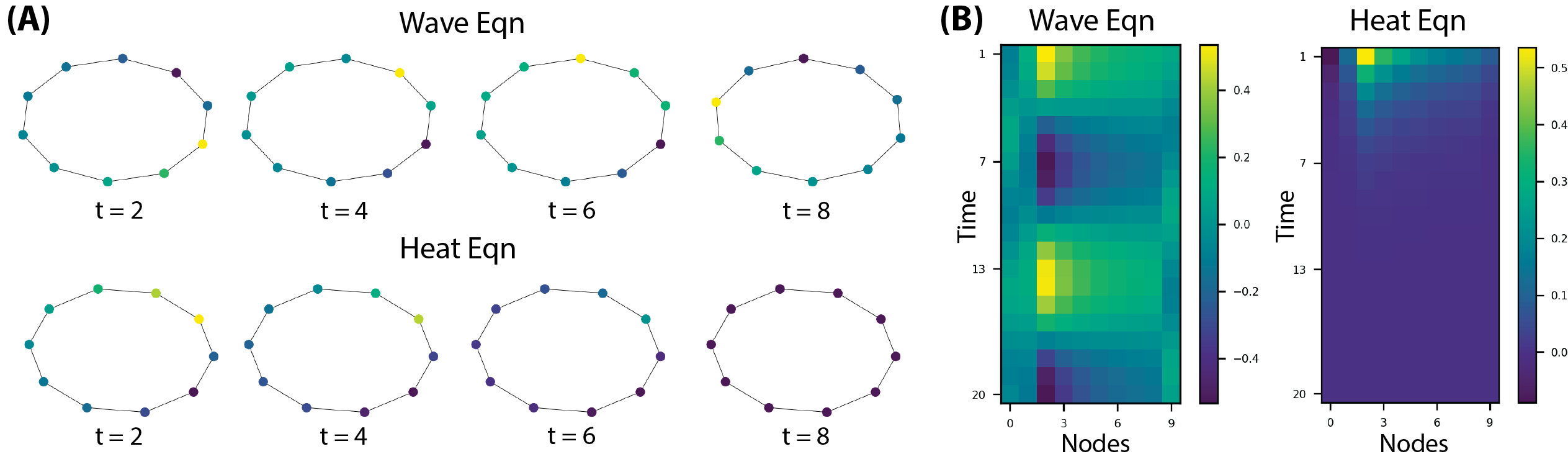
Fig. 1: (A) A cycle graph with nodes colored by the solution to the wave and heat equation. (B) Color map depicting the analytical solution to the wave and heat equation for all nodes on the cycle graph and $t=20$ time steps.

2.3 Properties of the Heat and Wave Equations

In this section, we present some theoretical results that demonstrate the connection between the behavior of the heat and wave equation and the graph topology. We begin by showing that the solutions remain on the connected components that the initial condition is supported on.

Proposition 2.3 (Connected components).

Suppose $G$ has $m$ connected components and partition the vertex set $V=V_{1}\sqcup V_{2}\sqcup\ldots\sqcup V_{m}$ where each $V_{i}$ is a connected component. Let $S$ be a set that is obtained by taking the union of several $V_{i}$’s, i.e., $S=V_{i_{1}}\sqcup\ldots\sqcup V_{i_{k}}$. Let $u(v,t)$ denote either $u_{H}(v,t)$ or $u_{W}(v,t)$ from (2) and (5) respectively. In the case of the heat equation (1), assume that the initial condition $\mathbf{x}$ has support contained in $S$. In the case of the wave equation (4), assume that both initial conditions $\mathbf{x}$ and $\mathbf{y}$ have support contained in $S$. Then for any $v\notin S$ and for all $t>0$, we have

$$u(v,t)=0.$$ (6)

Proof.

Let $v\notin S$. Observe that by relabelling nodes if necessary, the graph Laplacian may be written as:

$$L=\begin{pmatrix}\mathmakebox[1.8em]{L_{1}}\\ &\mathmakebox[1.8em]{\raise 4.0pt\hbox{.}\mkern 6.0mu\raise 1.0pt\hbox{.}\mkern 6.0mu\raise-2.0pt\hbox{.}}\\ &&\mathmakebox[1.8em]{L_{m}}\\ \end{pmatrix},$$

where each $L_{i}$ corresponds to the graph Laplacian for the individual connected component. Therefore, we may find an orthonormal basis of eigenvectors $\{\boldsymbol{\nu_{j}}\}_{j=1}^{n}$ such that the support of each $\boldsymbol{\nu_{j}}$ is contained in some $V_{i}$. Thus, for all $j$, we either have $\text{supp}(\boldsymbol{\nu_{j}})\subseteq S$, in which case $\boldsymbol{\nu_{j}}(v)=0$ or we have $\text{supp}(\boldsymbol{\nu_{j}})\cap S=\phi$, in which case $\langle\mathbf{x},\nu_{j}\rangle$ (and also $\langle\mathbf{y},\boldsymbol{\nu_{j}}\rangle$ in the case of the wave equation) will be zero. The result now follows from (2) and (5). ∎

The above proposition indicates that the behavior of heat and wave equations on a graph consisting of multiple connected components can be realized by considering the activity of the heat and wave equations on the individual connected components. Therefore, in the following propositions, we will restrict our discussion to connected graphs. We begin by considering the energy (in the squared norm sense) of solutions to the PDEs.

Proposition 2.4 (Heat energy).

Let $G$ be connected, and let $u_{H}(v,t)$ be as in (2) and let $u_{H}(t)=u_{H}(\cdot,t)$. Then,

$$e^{-2t\lambda_{n}}\|\mathbf{x}\|_{2}^{2}\leq\|u_{H}(t)\|_{2}^{2}\leq|\langle\boldsymbol{\nu_{1}},\mathbf{x}\rangle|^{2}+e^{-2t\lambda_{2}}\|\textbf{x}\|_{2}^{2}$$ (7)

for all $t>0$. The upper bound on heat energy obeys:

$$\|u_{H}(t)\|_{2}^{2}\leq\|\mathbf{x}\|_{2}^{2}=\|u_{H}(0)\|_{2}^{2}.$$ (8)

Additionally, as $t$ converges to infinity we have

$$\lim_{t\rightarrow\infty}u_{H}(t)=\langle\boldsymbol{\nu_{1}},\mathbf{x}\rangle\boldsymbol{\nu_{1}}.$$ (9)

Proof.

From (2), and the fact that $\{\boldsymbol{\nu_{i}}\}_{i=1}^{n}$ is an ONB, we see

$$\|u_{H}(t)\|_{2}^{2} =\sum_{i=1}^{n}e^{-2t\lambda_{i}}|\langle\boldsymbol{\nu_{i}},\mathbf{x}\rangle|^{2}.$$ (10)

$$=|\langle\boldsymbol{\nu_{1}},\mathbf{x}\rangle|^{2}+\sum_{i=2}^{n}e^{-2t\lambda_{i}}|\langle\boldsymbol{\nu_{i}},\mathbf{x}\rangle|^{2}$$

$$\leq|\langle\boldsymbol{\nu_{1}},\mathbf{x}\rangle|^{2}+e^{-2t\lambda_{2}}\sum_{i=2}^{n}|\langle\boldsymbol{\nu_{i}},\mathbf{x}\rangle|^{2}$$ (11)

$$\leq|\langle\boldsymbol{\nu_{1}},\mathbf{x}\rangle|^{2}+e^{-2t\lambda_{2}}\|\mathbf{x}\|_{2}^{2},$$

where (11) follows from the fact that $\lambda_{1}=0$. This establishes the upper bound in (7). Each of the remaining equations follow immediately from (10) and the fact that $0=\lambda_{1}<\lambda_{2}\leq\ldots\leq\lambda_{n}$. ∎

This proposition suggests that graphs with a larger $\lambda_{2}$ will have a faster rate of energy decay. The second eigenvalue of a graph can be related to the isoperimetric ratio of a graph through Cheeger’s inequality, thereby revealing information on graph structure and how “bottlenecked" a particular graph is [26]. There are cases where the energy decay is not fully controlled by $\lambda_{2}$. The following proposition controls for these cases and demonstrates that under certain conditions differences in the heat energy reflect structural differences between graphs:

Proposition 2.5 (Heat energy between graphs).

Let $G$ and $G^{\prime}$ be graphs on $n$ vertices with respective Laplacians $L_{G}$ and $L_{G^{\prime}}$ and let $\mathbf{x}$ and $\mathbf{x}^{\prime}$ be initial conditions for the heat equation (1) on $G$ and $G^{\prime}$ Then, under the following two assumptions:

1. $L_{G^{\prime}}\succcurlyeq L_{G}$, i.e.,

   $$\mathbf{v}^{T}L_{G^{\prime}}\mathbf{v}\geq\mathbf{v}^{T}L_{G}\mathbf{v}\>\>\text{for all }\mathbf{v}\in\mathbb{R}^{n}.$$

2. We have $\langle\boldsymbol{\nu_{i}^{\prime}},\mathbf{x^{\prime}}\rangle\leq(1+\delta_{i}(t))\langle\boldsymbol{\nu_{i}},\mathbf{x}\rangle$ for all $1\leq i\leq n,$ where we also assume $\delta_{i}(t):=e^{2t(\lambda_{i}^{\prime}-\lambda_{i})}-1\geq 0.$

Then, with $u_{H}$ and $u_{H}^{\prime}$ are defined as in (2), we have

$$\|u_{H}^{\prime}(t)\|^{2}_{2}\leq\|u_{H}(t)\|^{2}.$$ (12)

Proof.

$$\|u_{H}(t)\|_{2}^{2}-\|u_{H}^{\prime}(t)\|^{2}_{2}$$

$$\hskip 56.9055pt=\sum_{i=1}^{n}e^{-2t\lambda_{i}}|\langle\boldsymbol{\nu_{i}},\mathbf{x}\rangle|^{2}-e^{-2t\lambda_{i}^{\prime}}|\langle\boldsymbol{\nu_{i}^{\prime}},\mathbf{x^{\prime}}\rangle|^{2}$$

$$\hskip 56.9055pt\geq\sum_{i=1}^{n}\left[e^{-2t\lambda_{i}}-e^{-2t\lambda_{i}^{\prime}}(1+\delta_{i})\right]|\langle\boldsymbol{\nu_{i}},\mathbf{x}\rangle|^{2}$$

$$\hskip 56.9055pt=0.\qquad\quad\qquad\qquad\qquad\qquad\qquad\quad$$

∎

We note that Condition 1 of the lemma is satisfied if $G^{\prime}$ can be constructed from $G$ by the addition of edges or by increasing the weight of any edges (see, for example, Equation 1.1 of [26]). Condition 2 of the proposition may be satisfied by choosing $\mathbf{x}$ and $\mathbf{x}^{\prime}$ to be sum of all eigenvectors $\boldsymbol{\nu_{i}}$ and $\boldsymbol{\nu_{i}^{\prime}}$. Although this lemma represents a rather specific set of conditions, we expect that when two graphs have edges generated according to a similar rule or distribution, the more densely connected graph will have more rapidly decaying heat energy. An exploration of this is demonstrated in Figure 2 by examining the behavior of heat on Erdős-Rényi (ER) random graphs.

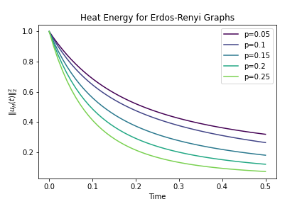
Fig. 2: $\|u_{H}(t)\|_{2}^{2}$ plotted for ER graphs with 25 nodes and probability of connection between nodes given by $p$. Average results are reported over 30 ER graphs for each $p$. For each graph a node is randomly selected to have a Dirac as the initial condition. It is observed that $\|u_{H}(t)\|_{2}^{2}$ decays more rapidly for ER graphs with a larger $p$.

Finally, we characterize the wave energy with the following proposition:

Proposition 2.6 (Wave energy).

Let $u_{W}(v,t)$ be the solution to the wave equation defined as in (3) and assume that $\mathbf{y=0}$ in (4). Then, for any $t\geq 0$, we have

$$|\langle\boldsymbol{\nu_{1}},\mathbf{x}\rangle|^{2}\leq\|u_{W}(t)\|_{2}^{2}\leq\|\mathbf{x}\|_{2}^{2}=\|u_{W}(0)\|_{2}^{2}.$$ (13)

Proof.

Similar to the proof of (7), we have

$$\|u_{W}(t)\|_{2}^{2} =\sum_{i=1}^{n}\cos^{2}(\sqrt{\lambda_{i}}t)|\langle\boldsymbol{\nu}_{i},\mathbf{x}\rangle|^{2}$$ (14)

$$\leq\ \sum_{i=1}^{n}|\langle\boldsymbol{\nu}_{i},\mathbf{x}\rangle|^{2}=\|\mathbf{x}\|_{2}^{2}.$$ (15)

The lower bound follows from combining (14) with the fact that $\lambda_{1}=0$.

∎

From (14), it is clear that unlike the heat energy which is non-increasing, the wave energy will oscillate over time. Thus, the wave equation may be well suited for capturing geometric features that are global in nature and require long-range interactions.

2.4 Heat-kernels and Random Walks

In the continuum, the solution to the heat equation is closely related to Brownian motion. In particular, if the initial condition is given by $u^{\text{continuum}}_{H}(\cdot,0)=\delta_{x_{0}}$, then $u^{\text{continuum}}_{H}(\cdot,t)$ is the probability distribution of a Brownian motion, starting from $x_{0}$, at time $t$. Therefore, intuitively, the solution to the graph heat equation (1) should be related to random walks.

Following a similar argument to Proposition 5.2 of [27], we consider the random-walk normalized Laplacian $L_{rw}:=I_{n}-D^{-1}A$. One may verify that it can be written in terms of the symmetric normalized Laplacian $L_{s}$ with $L_{rw}=D^{-1/2}L_{s}D^{1/2}$. Since $L_{s}$ is diagonalizable and can be written as $L_{s}=D^{-1/2}LD^{-1/2}=D^{-1/2}\Psi\Lambda\Psi^{-1}D^{-1/2}$, we see that $L_{rw}$ is also diagonalizable with $L_{rw}=S\Lambda S^{-1}$ where $S:=D^{-1/2}\Psi$. The random walk matrix $\mathbf{P}$ can be written as $\mathbf{P}=D^{-1}A=I_{n}-L_{rw}$. Therefore, we can write $\mathbf{P}^{t}=S(I_{n}-\Lambda)^{t}S^{-1}$.

Consider the heat kernel $\mathbf{U}^{t}_{H}$ defined as in (3) with $L=L_{rw}$ and note that $\mathbf{U}^{t}_{H}=Se^{-t\Lambda}S^{-1}$. We will show that $\mathbf{U}^{t}_{H}$ describes the transition probabilities of continuous-time random walker on the graph. Formally, we let $\{X_{i}\}_{i=1}^{\infty}$ be a random walk on the graph, let $\{N_{t}\}_{t\geq 0}$ be an ordinary, rate one, Poisson process, and let $\{X^{\text{continuous}}_{t}\}_{t\geq 0}$ be defined by $X^{\text{continuous}}_{t}=X_{N(t)}$.

Recalling that the probability mass function of a Poisson random variable with parameter $t$ is given by $p_{t}(k)=t^{k}e^{-t}/t!$, and for $t\geq 0$, we have

$$e^{-t(1-\mu)}=e^{-t}\sum_{k\geq 0}\frac{(t\mu)^{k}}{k!}=\sum_{k\geq 0}p_{t}(k)\mu^{k}.$$ (16)

Substituting $\lambda=1-\mu$ in (16) links the eigenvalues of $\mathbf{U}^{t}_{H}$ and $\mathbf{P}$ by

$$\mathbf{U}^{t}_{H} =Se^{-t\Lambda}S^{-1}=S\sum_{k\geq 0}p_{t}(k)(I_{n}-\Lambda)^{k}S^{-1}$$

$$=\sum_{k\geq 0}p_{t}(k)\mathbf{P}^{k}.$$

Therefore, we may interpret $\mathbf{U}^{t}_{H}(i,j)$ as the probability that a continuous-time random walker, which starts at $v_{i}$ will be located at $v_{j}$ at time $t$.

2.5 Capturing topological properties

In the following section, we will construct neural networks that use heat or wave dynamics as an aggregation scheme. Such networks present a promising and novel approach for predicting topological properties of graphs, including fundamental characteristics such as Betti numbers and curvature. These neural network architectures can harness the power of heat diffusion or wave propagation to encode the graph’s topology into continuous node representations. By modeling the dynamics of heat or wave propagation, these representations capture temporal evolution of node states, enabling the neural network to effectively learn and infer topological properties of the graph. Here, in this section, we will first give several examples of the topological properties which may be captured by these dynamics.

Example 2.7 (Connected Components).

In our experimental setup, we will consider the solutions to the heat equation with several different initial values $\mathbf{x}_{i}$ (and also $\mathbf{y}_{i}$ in the case of the wave equation). We will typically choose each $\mathbf{x}_{i}$ to be a rescaled Dirac $\delta$ function centered at a different node. By Proposition 2.3, each of the associated solutions PDE solutions $u_{H}^{(i)}$ and $u_{W}^{(i)}$ will have support contained within the connected component that contains the central node. (Moreover, inspecting the proof of Proposition 2.3, we see that the support will be equal to the entire connected component in the abscence of pathological cancellations.) Furthermore, analogous results approximately hold for nearly disconnected graphs such as a stochastic block model (SBM) with suitable parameters since for sufficiently small $t$ the energy of the input signal will not be able to spread from one cluster to another in significant quantities.

Example 2.8 ($u_{H}$ reveals distances and curvature).

In the settings of Riemannian manifolds, it is well-known that the heat kernel reveals geodesic distances via Varadhan’s formula [28] and is also closely related to Ricci curvature (see, for example, [29, 30]). In [31], it was shown that a modified version of Varadhan’s formula holds for graphs. This implies $u_{H}$ (and neural networks that utilize it) have the expressive power to characterize graph distances, and it also indicates that they have the power to characterize quantities derived from graph distances such as the Ollivier Ricci curvature (see, for example, [32]). Moreover, as discussed in Section 2.4, the solution to the heat equation is closely related to the behavior of a random walker on the graph. In [33], the transition probabilities of random walkers were used to construct another notion of curvature which the authors refer to as “diffusion curvature." Because the solutions of the heat-equation are fundamentally linked to the transitions of random walkers as discussed in Section 2.4, we anticipate that networks utilizing heat propagation will have the capacity to characterize the diffusion curvature of a graph as well.

Example 2.9 ($u_{W}$ reveals cycle lengths).

Unlike the solution to the heat equation, the $u_{W}$ is not localized in space and its energy does not decay uniformly as $t$ increases as shown in Figure 3.

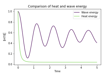
Fig. 3: $\|u(t)\|_{2}^{2}$ for the heat and wave equations over an ER graph (n = 25, p = 0.2) with Dirac initial condition.

Intuitively, this increases the ability of the wave equation to encode non-local topological structures such as cycle lengths and Betti numbers. This intuition is confirmed empirically in Table 1 where we observe that methods based on $u_{W}$ are more accurately able to predict extended persistence images than methods utilizing $u_{H}$ (or methods not using dynamics at all).

3 Methods

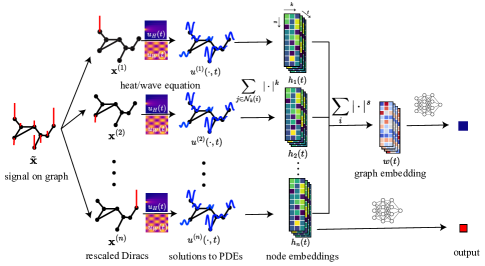
Fig. 4: The GDeNet architecture. Given an input signal on the graph, we first decompose it into $n$ Dirac signals. We then solve PDEs with these Diracs, and collect the results using statistical moments, to obtain the node embedding. We can further collect the node embeddings to form a graph embedding. Depending on the task type, the appropriate embedding is fed into an MLP to get the model output.

The GDeNet architecture contains two parts: The moment extractor and the neural network. The moment extractor solves the equations on the graph (with initial conditions derived from given input signals) and extracts statistical moments from these solutions. The neural network takes that representation as input and is trained for machine learning tasks.

3.1 Generation of Heat/Wave Node Representations

We solve each PDE with $n$ different initial conditions and use the solutions to generate the node representations. That is, in the case of the heat equation, we will solve the heat equation with $n$ different initial conditions $\mathbf{x}^{(i)},1\leq i\leq n$, and let $u_{H}^{(i)}$ be the associated solutions to (1). Similarly, in the wave equation case, we will consider initial conditions $\mathbf{x}^{(i)},\mathbf{y}^{(i)},1\leq i\leq n$, and let $u_{W}^{(i)}$ denote the associated solutions to (4). These signals are derived using an initial signal $\tilde{\mathbf{x}}$ defined on $V$.

We start by constructing the initial conditions $\mathbf{x}^{(i)},\mathbf{y}^{(i)}$. Suppose we are initially give a signal $\tilde{\mathbf{x}}\in\mathbb{R}^{n}$, (and also $\tilde{\mathbf{y}}\in\mathbb{R}^{n}$ in the wave case). For $1\leq i\leq n$, we define $\mathbf{x}^{(i)}=\tilde{\mathbf{x}}(v_{i})\delta_{v_{i}},$ (and similarly $\mathbf{y}^{(i)}=\tilde{\mathbf{y}}(v_{i})\delta_{v_{i}},$). $\mathbf{x}^{(i)}$ and $\mathbf{y}^{(i)}$ are to be thought of as Dirac signals on the $i$-th node rescaled by the initial signal evaluated at $v_{i}$. If the dataset does not have a signal $\tilde{\mathbf{y}}$, we set $\mathbf{y}^{(i)}=\mathbf{0}$ or $\mathbf{y}^{(i)}=\mathbf{x}^{(i)}$. Furthermore, if there is no initial signal in the dataset, we set $\mathbf{x}^{(i)}=\delta_{v_{i}}$.

Let $u^{(i)}(v,t)$ denote the solution to either the heat or the wave equation PDE, with the initial condition $u(\cdot,0)=\mathbf{x}^{(i)}$. We collect these solutions to a more compact tensor using statistical moments. For fixed parameters $K$ and $M$, the hidden representation of node $v_{i}$ at time $t$ is given by

$$h_{i}(t)=\Bigg{\{}\Big{\{}\sum_{j\in\mathcal{N}_{k}(i)}|u^{(i)}(v_{j},t)|^{m}\Big{\}}_{m=1}^{M}\Bigg{\}}_{k=2}^{K},$$ (17)

where $\mathcal{N}_{k}(i)$ denotes the set of vertices in the $k$-hop neighbors of vertex $v_{i}$. Using $T$ discrete time-steps, $t=1,2,\cdots,T$, we obtain a $M\times K\times T$ dimensional hidden representation for vertex $v_{i}$. (Our method can also be extended to the case where there are $r\geq 1$ initial signals, in which case we simply repeat this procedure $r$ times and then concatenate.)

3.2 From Node to Graph Representations

For graph-level tasks we calculate statistical moments over the node representations along the axis of the nodes as a means of pooling to get a graph representation.

$$w(t)=\Big{\{}\sum_{i=1}^{n}|h_{i}(t)|^{s}\Big{\}}_{s=1}^{S},$$ (18)

with a fixed $S$.

3.3 Neural Network

Depending on if the task is node-level or graph-level, we take the tensor $\Bigg{\{}\Big{\{}h_{i}(t)\Big{\}}_{t=1}^{T}\Bigg{\}}_{i=1}^{n}$ or $\Big{\{}w(t)\Big{\}}_{t=1}^{T}$, flatten it, and feed it into a multi-layer perceptron (MLP). This is the trainable part of GDeNet. In principle, other kinds of learning algorithms may be used depending on the particular task. For instance, if one wants to prioritize interpretability, one could utilize a decision tree classifier instead of an MLP.

3.4 Chebyshev Polynomials

Our implementation makes use of a Chebyshev polynomial approximation to compute the solutions to the heat and wave equations defined in (2) and (5) respectively. In doing so, we avoid eigendecomposing the Laplacian, which can have a computational complexity of $O(n^{3})$ [34]. The polynomial approximation has linear complexity (with respect to $n$) for sparse graphs [35]. For example, if $G$ is a $k$-nearest neighbor graph and the order of the polynomial is $m$, then the time complexity for solving the heat/wave equation is $O(kmn)$.

Table 1: Mean squared error (MSE, lower is better) for prediction of curvature and Betti numbers using GDeNet and a standard message-passing GNN with vertex degree as node features.

Graph	Properties		Ollivier-Ricci Curvature			Extended Persistence Image
	# Nodes	# Edges	GDeNet(W)	GDeNet(H)	MP-GNN	GDeNet(W)	GDeNet(H)	MP-GNN
$\text{ER}(p=0.04)$	$100$	$215$	1.93e-1	1.86e-1	32.04	6.53e-3	1.37e-2	8.34e-1
$\text{ER}(p=0.06)$		$313$	1.76e-1	1.80e-1	31.93	2.74e-3	8.82e-3	7.61e-1
$\text{ER}(p=0.08)$		$415$	1.79e-1	1.78e-1	31.87	1.96e-3	7.49e-3	1.07
$\text{ER}(p=0.04)$	$200$	$822$	3.58e-1	3.63e-1	18.09	4.49e-3	9.63e-3	5.11e-1
$\text{ER}(p=0.06)$		$1,228$	2.63e-1	3.19e-1	17.43	4.18e-3	7.87e-3	7.63e-1
$\text{ER}(p=0.08)$		$1,634$	2.57e-1	2.14e-1	15.50	1.83e-3	4.10e-3	9.93e-1
Cora [36]	$2,708$	$5,429$	1.85e-2	1.73e-2	0.24	7.36e-5	1.42e-4	2.83e-3
Citeseer [37]	$3,312$	$4,732$	3.41e-2	2.09e-2	0.22	1.55e-4	3.06e-4	7.39e-3
PubMed [38]	$19,717$	$44,338$	6.51e-3	7.30e-3	1.69	3.67e-3	8.18e-3	4.10e-1

Table 2: Mean squared error (MSE, lower is better) for the prediction of generating parameters of random graphs.

Method	Erdős-Rényi					Stochastic Block Model
	$n=100$	$n=250$	$n=500$	$n=1000$	$n=2500$	$n=100$	$n=250$	$n=500$	$n=1000$	$n=2500$
GDeNet(W)	8.29e-3	6.58e-3	3.17e-3	3.25e-3	1.04e-3	0.82	0.94	1.26	2.28	2.35
GDeNet(H)	7.46e-3	7.13e-3	3.60e-3	4.19e-3	3.04e-3	0.64	0.81	1.79	4.52	11.63
GCN	1.37e-2	1.14e-2	9.26e-3	9.49e-3	8.02e-3	2.93	3.07	3.68	7.14	10.26
GIN	1.08e-2	9.37e-3	7.74e-3	6.98e-3	4.81e-3	1.74	2.59	2.92	4.37	9.15

Table 3: R² score (higher is better) of GDeNet trained to predict molecular properties and molecular interactions. (Mean and standard deviation are calculated using $10$-fold cross-validation.)

Dataset	# Proteins	Property	Models
			GDeNet(W)	GDeNet(H)	GCN [4]	GAT [5]	GIN [6]
CASP5-13 [39]	$508$	Ramachandran	$\mathbf{0.87\pm 0.03}$	$0.74\pm 0.06$	$0.78\pm 0.01$	$0.72\pm 0.02$	$0.69\pm 0.03$
		Dihedral Angle	$\mathbf{0.93\pm 0.04}$	${0.90\pm 0.01}$	$0.83\pm 0.01$	$0.88\pm 0.04$	$0.81\pm 0.06$
		Bond Length	${0.96\pm 0.03}$	$\mathbf{0.98\pm 0.01}$	$0.89\pm 0.03$	$0.91\pm 0.01$	$0.93\pm 0.01$
		Torsion Angle	$\mathbf{0.63\pm 0.08}$	$0.58\pm 0.05$	$0.52\pm 0.04$	${0.60\pm 0.04}$	$0.51\pm 0.05$
DrugBank [40]	$12,416$	TPSA	$\mathbf{0.92\pm 0.01}$	$0.86\pm 0.02$	$0.71\pm 0.01$	$0.78\pm 0.02$	$0.69\pm 0.01$
		Num. Aromatic Rings	$\mathbf{0.96\pm 0.02}$	$0.85\pm 0.02$	$0.81\pm 0.01$	$0.83\pm 0.02$	$0.77\pm 0.01$

Table 4: 5-fold cross-validation accuracy (higher is better) of GDeNet on biomolecular datasets in the TUDatasets benchmark [41]

Dataset	# Proteins	# Classes	Models
			GDeNet(W)	GDeNet(H)	GCN	GAT	GIN
ENZYMES [42, 43]	600	6	$\mathbf{0.727\pm 0.003}$	$0.639\pm 0.006$	$0.497\pm 0.004$	$0.584\pm 0.002$	$0.613\pm 0.004$
PROTEINS [44, 43]	1113	2	$\mathbf{0.826\pm 0.004}$	$0.795\pm 0.002$	$0.713\pm 0.004$	$0.779\pm 0.010$	$0.743\pm 0.005$
MUTAG [45, 46]	187	2	$\mathbf{0.974\pm 0.003}$	$0.966\pm 0.002$	$0.931\pm 0.003$	$0.927\pm 0.002$	$0.873\pm 0.005$

4 Empirical Results

4.1 Recovery of geometric and topological properties

We empirically assessed the expressivity of the wave equation and the heat equation solutions as replacements for message passing on graphs by training our network to recover geometric and topological properties. We trained the network to perform two regression tasks: predicting the Ollivier-Ricci curvature [47], and predicting the persistence image representation [48] of the extended persistence diagram.

In Riemannian geometry, Ricci curvature measures how much the manifold deviates from being Euclidean along the tangent directions. Analogously, in the discrete setting, Ollivier-Ricci curvature captures the local geometry of the graph. The extended persistence diagram is obtained from ascending and descending filtrations of the $5$-hop neighborhood graphs at each node, using node degree as the filter function (see, e.g., [49, 50] for further details). We trained and tested the model on both synthetic data, consisting of Erdős-Rényi graphs, $G(n,p)$, with $n=\{100,200\}$ vertices and $p=\{0.04,0.06,0.08\}$ edge probabilities as well as three citation graphs, (Cora, Citeseer, and PubMed) which are commonly used as benchmark datasets (Table 1).

PDE solutions were computed by placing a Dirac $\delta$ at each node and computing the moments of the PDE solution across the nodes at various timepoints according to (17) and (18). We use a 5-layer feed-forward network to predict the Ricci curvature at each node after computing the moments. We trained a 12-layer feed-forward network, using the concatenation of moments across all nodes as the input, to predict the extended persistence image, consisting of connected components (dimension $0$ homology) and topological loops (dimension $1$ homology). In addition, we compared our network to a more standard message-passing GNN trained using the node degree as input features.

Our results demonstrate that using moments obtained from the solutions to the heat equation and the wave equation as node features in lieu of message-passing results in higher prediction accuracy of Ollivier-Ricci curvature and the extended persistence of graphs compared to conventional message-passing GNNs (Table 1). In particular, both the methods based on $u_{W}$ and on $u_{H}$ outperformed standard message passing on both the real-world and synthetic datasets.

Next, we considered the task of recovering the structure of random graphs generated using the ER model and the SBM. ER graphs were generated with edge probabilities ranging from $0.01$ to $0.1$. SBM graphs containing between $5$ to $25$ different communities were generated, with the probability of edges between nodes within a community set to $0.5$ and the probability of edges between nodes in different communities set to $0.05$. Specifically, we compared GDeNet to GCN and GIN in the task of recovering the generative parameters for these models, namely the probability of connecting two nodes by an edge in the ER model and the number of blocks/communities in the SBM. As shown in Table 2, GDeNet outperformed both GCN and GIN in this task, demonstrating the expressivity of PDE solutions and the ability to identify the generative process underlying random graph construction.

4.2 Molecular Graph Classification and Property Prediction

To demonstrate the predictive power of GDeNet in the real-world setting, we conducted experiments with molecular graphs representing proteins and drug-like molecules [39, 40, 41]. The geometry and topology of proteins are defined by the arrangement of their amino acid residues in the three-dimensional space. The dihedral and torsion angles define the rotation of the amino acid residues around the bonds, and hence, influence the overall fold and shape of the protein. The Ramachandran density plot encodes the allowed and disallowed regions of dihedral angles for the amino acid residues in a protein, thus representing the possible conformations of the protein backbone. As shown in Table 3, GDeNet outperforms GCN, GAT, and GIN in predicting the shape of the protein using these parameters.

We also compared GDeNet with other graph neural networks in predicting two important properties that influence their biological activity and pharmacokinetics of drug-like molecules. The total polar surface area (TPSA) is the surface area occupied by polar atoms (oxygen, nitrogen, and attached hydrogens) in a molecule. TPSA is related to the ability of a molecule to cross biological membranes, like the blood-brain barrier, and is therefore, an important factor in drug design. Polar atoms and groups in a molecule tend to orient themselves in a way that minimizes the energy and maximizes interactions with the solvent or other molecules. The larger the TPSA, the more polar the molecule is, which in turn affects its three-dimensional structure and its interaction with biological targets. Aromatic rings are planar, cyclic structures containing alternating single and double bonds. The presence of aromatic rings in a molecule contributes to its rigidity and flatness. Aromatic rings tend to stack on top of each other through $\pi-\pi$ bond interactions, influencing the overall shape and size of the molecule. Furthermore, the presence of aromatic rings increases the hydrophobicity of the molecule, which can influence its solubility and interaction with biological targets. Therefore, a higher TPSA often results in a more branched and less compact molecule, while a higher number of aromatic rings often results in a more planar and rigid molecule. As shown in Table 3, GDeNet trained using the dynamics of the wave equation on molecular graphs, outperforms GCN, GAT, and GIN in predicting TPSA and the number of aromatic rings in drug-like molecules.

In addition, we evaluated the performance of GDeNet on three publicly available datasets for biomolecular graph classification from the TUDatasets benchmark [41]. The ENZYMES dataset [42] consists of protein secondary structures with ground truth annotations of catalytic activity. In the PROTEINS dataset [44], the task is to classify whether a protein functions as an enzyme. The MUTAG dataset [45], contains small nitroaromatic compounds, and the task is to classify their mutagenicity on the S.typhimurium bacterium. The GDeNet achieved high validation accuracy on these models (Table 4), with the wave equation outperforming other models on all datasets.

5 Conclusion

We have introduced GDeNet, a neural network which utilizes moments extracted from the dynamics of heat and wave propagation to infer the geometric and topological properties of a network. Our method is based upon (i) solving a semi-discrete PDE on a graph, (ii) extracting statistical moments from the solution to the PDE, and (iii) training a multi-layer perceptron on top of these statistical moments. We provide a theoretical analysis showing that these dynamics are related to the connectivity of the graph, several notions of curvature, as well as other properties such as cycle lengths. In our numerical experiments, we demonstrate that our method is effective for predicting these topological properties as well as generating parameters of random graphs drawn from different families.

References

- [1] Antonio Ortega, Pascal Frossard, Jelena Kovačević, José MF Moura, and Pierre Vandergheynst, “Graph signal processing: Overview, challenges, and applications,” Proceedings of the IEEE, vol. 106, no. 5, pp. 808–828, 2018.
- [2] Robert Geroch, “Partial differential equations of physics,” in General Relativity, pp. 19–60. Routledge, 2017.
- [3] Xiaowen Dong, Dorina Thanou, Laura Toni, Michael Bronstein, and Pascal Frossard, “Graph signal processing for machine learning: A review and new perspectives,” IEEE Signal processing magazine, vol. 37, no. 6, pp. 117–127, 2020.
- [4] Thomas N. Kipf and Max Welling, “Semi-supervised classification with graph convolutional networks,” in 5th International Conference on Learning Representations, 2017.
- [5] Petar Velickovic, Guillem Cucurull, Arantxa Casanova, Adriana Romero, Pietro Lio, Yoshua Bengio, et al., “Graph attention networks,” stat, vol. 1050, no. 20, pp. 10–48550, 2017.
- [6] Keyulu Xu, Weihua Hu, Jure Leskovec, and Stefanie Jegelka, “How powerful are graph neural networks?,” in 7th International Conference on Learning Representations, ICLR, 2019.
- [7] Reijneveld et al., “The application of graph theoretical analysis to complex networks in the brain,” Clinical neurophysiology, 2007.
- [8] Boccaletti et al., “The structure and dynamics of multilayer networks,” Physics reports, vol. 544, no. 1, pp. 1–122, 2014.
- [9] Joana A Simoes, “An agent-based/network approach to spatial epidemics,” Agent-based models of geographical systems, 2011.
- [10] Petter Holme and Jari Saramäki, “Temporal networks,” Physics reports, vol. 519, no. 3, pp. 97–125, 2012.
- [11] Filipe De Avila Belbute-Peres, Thomas Economon, and Zico Kolter, “Combining differentiable pde solvers and graph neural networks for fluid flow prediction,” in international conference on machine learning. PMLR, 2020, pp. 2402–2411.
- [12] Alvaro Sanchez-Gonzalez, Jonathan Godwin, Tobias Pfaff, Rex Ying, Jure Leskovec, and Peter Battaglia, “Learning to simulate complex physics with graph networks,” in International conference on machine learning. PMLR, 2020, pp. 8459–8468.
- [13] Tobias Pfaff, Meire Fortunato, Alvaro Sanchez-Gonzalez, and Peter W Battaglia, “Learning mesh-based simulation with graph networks,” arXiv:2010.03409, 2020.
- [14] Benjamin Chamberlain, James Rowbottom, Davide Eynard, Francesco Di Giovanni, Xiaowen Dong, and Michael Bronstein, “Beltrami flow and neural diffusion on graphs,” Advances in Neural Information Processing Systems, vol. 34, pp. 1594–1609, 2021.
- [15] Ben Chamberlain, James Rowbottom, Maria I Gorinova, Michael Bronstein, Stefan Webb, and Emanuele Rossi, “Grand: Graph neural diffusion,” in International Conference on Machine Learning, 2021.
- [16] P. Goyal, S. Chhetri, and A. Canedo, “dyngraph2vec: Capturing network dynamics using dynamic graph representation learning,” Knowledge-Based Systems, vol. 187, pp. 104816, 2020.
- [17] George W Bluman and Julian D Cole, “The general similarity solution of the heat equation,” Journal of mathematics and mechanics, 1969.
- [18] John R Cannon, “The solution of the heat equation subject to the specification of energy,” Quarterly of Applied Mathematics, vol. 21, no. 2, pp. 155–160, 1963.
- [19] Tariq Alkhalifah, “An acoustic wave equation for anisotropic media,” Geophysics, vol. 65, no. 4, pp. 1239–1250, 2000.
- [20] Roger K Dodd, J Chris Eilbeck, John D Gibbon, and Hedley C Morris, “Solitons and nonlinear wave equations,” Academic Press, Inc.[Harcourt Brace Jovanovich, Publishers], London-New York …, 1982.
- [21] Matthias Erbar, “The heat equation on manifolds as a gradient flow in the wasserstein space,” Annales de l’IHP Probabilités et statistiques, vol. 46, no. 1, pp. 1–23, 2010.
- [22] Yiming Jiang, Xingchun Wang, and Yongjin Wang, “On a stochastic heat equation with first order fractional noises and applications to finance,” Journal of Mathematical Analysis and Applications, 2012.
- [23] Lu Liu, Etienne Vincent, Xu Ji, Fuhao Qin, and Yi Luo, “Imaging diffractors using wave-equation migration,” Geophysics, 2016.
- [24] Benjamin T Cox, S Kara, Simon R Arridge, and Paul C Beard, “k-space propagation models for acoustically heterogeneous media: Application to biomedical photoacoustics,” The Journal of the Acoustical Society of America, vol. 121, no. 6, pp. 3453–3464, 2007.
- [25] Joyce Chew, Matthew Hirn, Smita Krishnaswamy, Deanna Needell, Michael Perlmutter, Holly Steach, Siddharth Viswanath, and H.T. Wu, “Geometric scattering on measure spaces,” arXiv:2208.08561, 2022.
- [26] Daniel A Spielman, “Spectral and algebraic graph theory, 2019,” URL http://cs-www. cs. yale. edu/homes/spielman/sagt. Version dated December, vol. 19, 2019.
- [27] Guillaume Huguet, Alexander Tong, Edward De Brouwer, Yanlei Zhang, Guy Wolf, Ian Adelstein, and Smita Krishnaswamy, “A heat diffusion perspective on geodesic preserving dimensionality reduction,” 2023.
- [28] Sathamangalam R Srinivasa Varadhan, “On the behavior of the fundamental solution of the heat equation with variable coefficients,” Communications on Pure and Applied Mathematics, vol. 20, no. 2, pp. 431–455, 1967.
- [29] Mathias Braun and Chiara Rigoni, “Heat kernel bounds and Ricci curvature for lipschitz manifolds,” 2021.
- [30] Richard H. Bamler and Qi S. Zhang, “Heat kernel and curvature bounds in Ricci flows with bounded scalar curvature,” Advances in Mathematics, vol. 319, pp. 396–450, 2017.
- [31] Keenan Crane, Clarisse Weischedel, and Max Wardetzky, “The heat method for distance computation,” Commun. ACM, vol. 60, no. 11, pp. 90–99, Oct. 2017.
- [32] Florentin Münch and Radosław K. Wojciechowski, “Ollivier Ricci curvature for general graph Laplacians: Heat equation, Laplacian comparison, non-explosion and diameter bounds,” Advances in Mathematics, vol. 356, pp. 106759, 2019.
- [33] Bhaskar et al., “Diffusion curvature for estimating local curvature in high dimensional data,” 2022.
- [34] David K Hammond, Pierre Vandergheynst, and Rémi Gribonval, “Wavelets on graphs via spectral graph theory,” Applied and Computational Harmonic Analysis, vol. 30, no. 2, pp. 129–150, 2011.
- [35] Michaël Defferrard, Xavier Bresson, and Pierre Vandergheynst, “Convolutional neural networks on graphs with fast localized spectral filtering,” Advances in neural information processing systems, 2016.
- [36] Andrew Kachites McCallum, Kamal Nigam, Jason Rennie, and Kristie Seymore, “Automating the Construction of Internet Portals with Machine Learning,” Information Retrieval, vol. 3, no. 2, July 2000.
- [37] C. Lee Giles, Kurt D. Bollacker, and Steve Lawrence, “CiteSeer: an automatic citation indexing system,” in Proceedings of the third ACM conference on Digital libraries, May 1998.
- [38] Sen et al., “Collective Classification in Network Data,” AI Magazine, vol. 29, no. 3, Sept. 2008, Number: 3.
- [39] Andriy Kryshtafovych, Torsten Schwede, Maya Topf, Krzysztof Fidelis, and John Moult, “Critical assessment of methods of protein structure prediction (CASP)-Round XIII,” Proteins, 2019.
- [40] D Wishart et al., “DrugBank 5.0: a major update to the DrugBank database for 2018,” Nucleic Acids Research, vol. 46, no. D1, pp. D1074–D1082, Jan. 2018.
- [41] C. Morris, N. Kriege, F. Bause, K. Kersting, P. Mutzel, and M. Neumann, “Tudataset: A collection of benchmark datasets for learning with graphs,” arXiv:2007.08663, 2020.
- [42] Schomburg et al, “BRENDA, the enzyme database: updates and major new developments,” Nucleic Acids Research, , no. suppl_1, Jan. 2004.
- [43] Borgwardt et al., “Protein function prediction via graph kernels,” Bioinformatics (Oxford, England), pp. 47–56, June 2005.
- [44] Paul D. Dobson and Andrew J. Doig, “Distinguishing enzyme structures from non-enzymes without alignments,” Journal of Molecular Biology, vol. 330, no. 4, pp. 771–783, July 2003.
- [45] Debnath et al., “Structure-activity relationship of mutagenic aromatic and heteroaromatic nitro compounds. correlation with molecular orbital energies and hydrophobicity,” Journal of medicinal chemistry, vol. 34, no. 2, pp. 786–797, 1991.
- [46] Nils Kriege and Petra Mutzel, “Subgraph matching kernels for attributed graphs,” in Proceedings of the 29th International Conference on International Conference on Machine Learning, 2012, ICML’12.
- [47] Yann Ollivier, “Ricci curvature of Markov chains on metric spaces,” July 2007, arXiv:math/0701886.
- [48] H. Adams, S. Chepushtanova, T. Emerson, E. Hanson, M. Kirby, F. Motta, R. Neville, C. Peterson, P. Shipman, and L. Ziegelmeier, “Persistence Images: A Stable Vector Representation of Persistent Homology,” 2016, arXiv:1507.06217.
- [49] David Cohen-Steiner, Herbert Edelsbrunner, and John Harer, “Extending Persistence Using Poincaré and Lefschetz Duality,” Foundations of Computational Mathematics, vol. 9, no. 1, pp. 79–103, Feb. 2009.
- [50] Zuoyu Yan, Tengfei Ma, Liangcai Gao, Zhi Tang, Yusu Wang, and Chao Chen, “Neural Approximation of Graph Topological Features,” Nov. 2022, arXiv:2201.12032 [cs].