Quantum Vision Clustering

Abstract

Unsupervised visual clustering has garnered significant attention in recent times, aiming to characterize distributions of unlabeled visual images through clustering based on a parameterized appearance approach. Alternatively, clustering algorithms can be viewed as assignment problems, often characterized as NP-hard, yet precisely solvable for small instances on contemporary hardware. Adiabatic quantum computing (AQC) emerges as a promising solution, poised to deliver substantial speedups for a range of NP-hard optimization problems. However, existing clustering formulations face challenges in quantum computing adoption due to scalability issues. In this study, we present the first clustering formulation tailored for resolution using Adiabatic quantum computing. An Ising model is introduced to represent the quantum mechanical system implemented on AQC. The proposed approach demonstrates high competitiveness compared to state-of-the-art optimization-based methods, even when utilizing off-the-shelf integer programming solvers. Lastly, this work showcases the solvability of the proposed clustering problem on current-generation real quantum computers for small examples and analyzes the properties of the obtained solutions.

1 Introduction

Unsupervised learning in automated object and human understanding has recently become one of the most popular research topics in robot vision. It is primarily due to the abundance of unlabelled raw data and the need for robust visual recognition algorithms that can perform consistently in various challenging conditions. However, traditional methods, like K-Mean clustering, have shown limitations regarding speed and accuracy when dealing with large-scale databases. These methods heavily rely on a predetermined number of clusters ($k$), which is not applicable in real scenarios, such as a visual object or visual landmark recognition clustering. In recent years, several studies [1, 2, 3] based on deep learning have been proposed to address the challenge of unsupervised clustering. However, these methods still rely on rule-based algorithms for the final cluster construction, and since they need to process large-scale databases, this step still needs to be completed.

In this paper, we will map the clustering problem into a quantum mechanical system whose energy is equivalent to the cost of the optimization problem. Therefore, if it is possible to measure the lowest energy state of the system, a solution to the corresponding optimization problem is found. It is done with an Adiabatic Quantum Computer (AQC), which implements a quantum mechanical system made from qubits and can be described by the Ising model. Using this approach, a quantum speedup, which further scales with system size and temperature, has already been shown for applications in physics.

While quantum computing can provide a range of future advantages, mapping a problem to an AQC is nontrivial. It often requires reformulating the problem from scratch, even for well-investigated tasks. On the one hand, the problem needs to be matched to the Ising model. On the other hand, real quantum computers have a minimal number of qubits and are still prone to noise, which requires tuning the model to handle the limitations. In this work, we present the first quantum computing approach for visual clustering.

Principal Contributions: In this work, we introduce a novel visual clustering approach using quantum machine learning. Our principal contributions can be summarized as follows:

• Initially, we formulate the clustering problem as a Quadratic Unconstrained Binary Optimization (QUBO) problem. Different from previous methods, our formulation can work even number of clusters is unspecified.

• Lastly, we present an efficient solution approach for this QUBO problem using Adiabatic Quantum Computing, aiming to attain promising unsupervised clustering outcomes.

Throughout the rest of this paper, we will present related studies addressing the visual clustering problem. Subsequently, we articulate the visual clustering problem within the quantum framework. This will be followed by an exploration of fundamental concepts in quantum computing. We will then detail our approach to framing the visual clustering problem through a QUBO formulation. Lastly, we demonstrate the outcomes of our experiments conducted on the D-Wave quantum computer and draw comparisons with the $k$-NN clustering algorithm.

2 Related Work

Quantum Machine Learning: Quantum machine learning algorithms have been recently developed to solve problems that are too slow to solve on classical computers. Examples include Shor’s Algorithm to factor large integers [4], Grover’s Algorithm for searching [5], and the Deutsch-Josza algorithm for determining whether a black box function is constant or balanced [6].

A class of discrete optimization problems known as Quadratic Unconstrained Binary Optimization problems is particularly amenable to a technique known as Adiabatic Quantum computing. This paper investigates how classical computing and Adiabatic Quantum computing can be unified to solve the Visual Clustering problem by formulating it in an end-to-end QUBO framework. Prior studies have used the strategy of solving QUBO problems with Adiabatic Quantum computing for tasks like cluster assignment, robust fitting, and $k$-means clustering. [7, 8, 9]

Deep Visual Clustering: Visual clustering is a crucial tool for data analytics. Deep visual clustering refers to applying deep learning methods to clustering. Classical techniques for clustering such as density-based clustering, centroid-based clustering, distribution-based clustering, ensemble clustering, etc. [10] display limited performance on complex datasets. Deep neural networks seek to map complex data to a feature space where it becomes easier to cluster. [10] Modern deep clustering methods have focused on Graph Convolutional Neural Networks (GCN) and Transformers [11, 12, 13].

Empirical data is often most naturally represented with a graph structure. For example, websites are usually connected by a hyperlink. Social media platform users are connected by being followers or stores connected by roads. GCNs exploit this graph structure by taking it as input to produce more accurate features, which are used finally to cluster the nodes. [14, 15, 16, 17] Transformers also exploit the connections between the data; Ling et al. unified for the first time the transformer model and contrastive learning for image clustering. [13] Nguyen et al. presented the Clusformer model, which addresses the sensitivity of the GCN to noise and uses a transformer for the task of visual clustering [18].

3 Preliminaries on Quantum Computing

3.1 Quantum Bit (Qubit)

A qubit in a quantum computer has the role as the analog of a bit in a classical computer. Mathematically, a qubit $q$ is a vector in a two-dimensional complex vector space spanned by the basis vectors $\ket{0}=[1,0]^{T}$ and $\ket{1}=[0,1]^{T}$:

$$q=\alpha\ket{0}+\beta\ket{1}$$

such that $|\alpha|^{2}+|\beta|^{2}=1$. Physically, a qubit can be realized as the different energy levels of an atom, polarizations of a photon, ions trapped in an electromagnetic stasis, and more. [19]

3.2 Quantum Superposition

A qubit is in quantum superposition if its state cannot be expressed as a single-scaled basis vector [19]. For example, qubit $q_{1}$ is in quantum superposition and qubit $q_{2}$ is not in the following equations:

$$\begin{split}q_{1}&=\ket{0}\\ q_{2}&=\frac{1}{\sqrt{2}}\ket{0}+\frac{1}{\sqrt{2}}\ket{1}\end{split}$$

3.3 Measurement

Measurement of a qubit $q$ with respect to the basis $\{\ket{0},\ket{1}\}$ causes the state of $q$ to change to exactly one of $\ket{0},\ket{1}$. In particular, if $q$ is in the state:

$$q=\alpha\ket{0}+\beta\ket{1}$$

then upon measurement, $q$ will collapse into state $\ket{0}$ with probability $|\alpha|^{2}$ and state $\ket{1}$ with probability $|\beta|^{2}$ [19].

3.4 Entanglement

The state of a two-qubit system $q_{0},q_{1}$ is a vector in the tensor product of their respective state vector spaces [19]. Therefore, if we use $\ket{0},\ket{1}$ as the basis for each of the state vector spaces of $q_{0},q_{1}$ respectively, then the basis for the state vector space of the two-qubit system is $\{\ket{0}\otimes\ket{0},\ket{0}\otimes\ket{1},\ket{1}\otimes\ket{0},\ket{1}\otimes\ket{1}\}$. If two qubits $q_{0},q_{1}$ have a state that cannot be represented as a complex scalar time basis vector. Then they are said to be entangled. For example, an example of an unentangled two-qubit state can be presented as follows,

$$-i\ket{1}\otimes\ket{0}$$

and an example of an entangled two-qubit state is presented as follows,

$$\frac{1}{\sqrt{2}}\ket{0}\otimes\ket{0}-\frac{1}{\sqrt{2}}\ket{1}\otimes\ket{1}$$

Likewise, the state of an $n$-qubit system is a vector in the tensor product of their respective state vector spaces. For ease of reading, it is convention to represent the tensor product of basis vectors in the following form:

$$\ket{b_{1}}\otimes\cdot\cdot\cdot\otimes\ket{b_{n}}=\ket{b_{1}...b_{n}}$$

where $\ket{b_{i}}$ is a basis vector in the state vector space of qubit $q_{i}$.

3.5 Adiabatic Quantum Computing

The quantum state $\ket{\psi(t)}$ of a system of qubits varies with time according to the Schrödinger equation:

$$i\frac{\partial}{\partial t}\ket{\psi(t)}=H(t)\ket{\psi(t)}$$

where $H(t)$ is an operator called the Hamiltonian of the quantum system. At each time $t$, $H(t)$ describes the energy of the quantum state. Encoding the QUBO problem in a Hamiltonian $H_{QUBO}(t)$ means that the answer is the state of the qubits when $H_{QUBO}(t)$ is in the lowest energy state. Initializing $H_{QUBO}$ in its lowest energy state is problematic because it is complex. Many researchers use the strategy of Adiabatic Quantum Computing to compute the lowest energy state of a complex quantum system, which is where we initialize the quantum system in the lowest energy state of some easy-to-compute Hamiltonian $H_{BASIC}$, and form our Hamiltonian as the interpolation between them:

$$H(t)=(1-t/T)H_{BASIC}(t)+(t/T)H_{QUBO}(t)$$

The Adiabatic Theorem states that as long as $0\leq t\leq T$ is varied slowly enough, $H$ will remain in its ground state throughout the interval $[0,T]$, so when we measure the quantum state at time $T$, the system will be in its ground state and satisfy the QUBO problem [20].

4 Deep Visual Clustering

Let $\mathcal{D}$ be a set of $N$ data points to be clustered. We define $\mathcal{H}:\mathcal{D}\rightarrow\mathcal{X}\subset\mathbb{R}^{N\times d}$ as a function that embeds these data points to a latent space $\mathcal{X}$ of $d$ dimensions. Let $\hat{Y}$ be a set of ground-truth cluster IDs assigned to the corresponding data points. Since $\hat{Y}$ has a maximum of $N$ different cluster IDs, we can represent $\hat{Y}$ as a vector of $\left[0,N-1\right]^{N}$. A deep clustering algorithm $\Phi:\mathcal{X}\rightarrow Y\in\left[0,N-1\right]^{N}$ is defined as a mapping that maximizes a clustering metric $\sigma(Y,\hat{Y})$.

As $\hat{Y}$ is not accessible during the training stage, the number of clusters and samples per cluster are not given beforehand. Therefore, divide and conquer philosophy can be adapted to relax the problem. In particular, a deep clustering algorithm $\Phi$ can be divided into three sub-functions: pre-processing $\mathcal{K}$, in-processing $\mathcal{M}$, and post-processing $\mathcal{P}$ functions. Formally, $\Phi$ can be presented as in Eqn. (1).

$$\Phi(\mathcal{X})=\{\mathcal{M}\circ\mathcal{K}(\mathbf{x}_{i},n)\}_{\mathbf{x}_{i}\in\mathcal{X}}$$ (1)

where $\mathcal{K}$ denotes an unsupervised clustering algorithm on deep features $\mathbf{x}_{i}$ of the $i$-th sample. k-NN is usually a common choice for $\mathcal{K}$ [2, 1, 21, 22, 3].

In addition, for the post-processing $\mathcal{P}$ function, it is usually a rule-based algorithm to merge two or more clusters into one when they share high concavities [1, 2, 21]. Since $\mathcal{P}$ does not depend on the input data points nor is a learnable function, the parameters $\theta_{\mathcal{M}}$ of $\Phi$ can be optimized via this objective function:

$$\theta^{*}_{\mathcal{M}}=\arg\min_{\theta_{\mathcal{M}}}\mathbb{E}_{\mathbf{x}_{i}\sim p(\mathcal{X})}\left[\mathcal{L}(\mathcal{M}\circ\mathcal{K}(\mathbf{x}_{i},n),\hat{q}_{i})\right]$$ (2)

where $k$ is the number of the nearest neighbors of input $\mathbf{x}_{i}$, $\hat{q_{i}}$ is the objective of $\mathcal{M}$ to be optimized, and $\mathcal{L}$ denotes a suitable clustering or classification loss.

Given that the clustering method typically consists of three components, namely $\mathcal{K}$, $\mathcal{M}$, and $\mathcal{P}$, previous studies primarily concentrated on enhancing the performance of $\mathcal{M}$. However, the $\mathcal{P}$ also holds an important role contributing to the overall performance [18]. In most studies [18, 23, 24], the design of $\mathcal{P}$ is typically addressed with a simple rule-based algorithm, which often proves to be sensitive and reliant on the threshold chosen. Consequently, this sensitivity significantly impacts the overall performance of the clustering system, rendering it unstable. In this paper, we thoroughly investigate the design of $\mathcal{P}$ from an optimization perspective. To address this challenge, we propose a novel approach that leverages quantum machine techniques, improving unsupervised clustering performance.

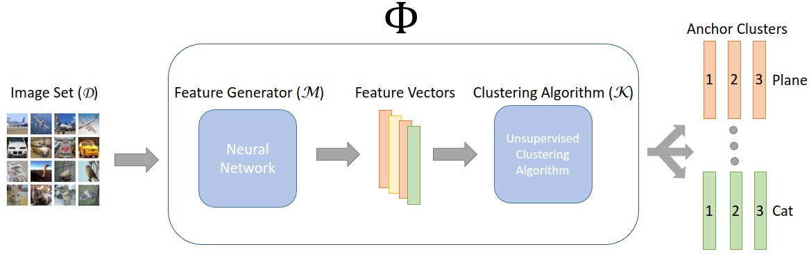
Figure 1: A visualization of the problem formulation that shows the flow of images from the image set to their final assignment to an anchor cluster.

5 Our Proposed Method

5.1 QUBO Formulation

In this section, we formulate the $\mathcal{P}$ component from the optimization perspective. Given a set of clusters $\mathcal{G}=\{g_{0},g_{1},\dots,g_{u-1}\}$. It is noted that $g_{i}=\mathcal{M}(\mathcal{K}(\mathbf{x}_{i},n)$) is processed by deep network $\mathcal{M}$ to remove the noisy samples, thus, number of samples in each cluster $|g_{i}|$ can vary among clusters. The objective of $\mathcal{P}$ can be defined as in Eqn. (3).

$$\mathbf{max}\sum_{i,j}^{u}\mathbbm{1}_{c_{i}=c_{j}}$$ (3)

where $\mathbbm{1}$ is the indicator function, $c_{i}$ is the cluster id of cluster $g_{i}$. Typically, the $c_{i}$ can be determined by the centroid $\mathbf{x}_{i}$. This information is available in the training phase, but in the testing phase. For this reason, $\mathcal{P}$ has to determine which clusters share the same ID. To address this problem, we find the optimal solution of Eqn. (3) using the Quadratic Unconstrained Binary Optimization Problem.

We can divide the $\mathcal{G}$ into two sets of clusters, denoted as $\mathcal{A}$ and $\mathcal{B}$. Let $\mathcal{A}=\{\textbf{a}_{1},\textbf{a}_{2},\dots\textbf{a}_{r}\}$ be a set of anchor clusters where each individual cluster $\textbf{a}_{i}$ is assigned a distinct ID. Let $\mathcal{B}=\{\textbf{b}_{1},\textbf{b}_{2},\dots\textbf{b}_{s}\}$ be the set of unknown clusters where we do not know their IDs. Our goal is to assign $\textbf{b}_{j}$ to a cluster $\textbf{a}_{i}$ if they share the same ID or add $\textbf{b}_{j}$ to be a new element of $\mathcal{A}$ if it does not match with any cluster inside $\mathcal{A}$. Formally, let $\mathbf{u}\in\mathbbm{R}^{r\times s}$ be the binary matrix where,

$$\textbf{u}_{ij}=\begin{cases}1&\textbf{b}_{j}\text{ matches to }\textbf{a}_{i}\\ 0&\text{ otherwise }\end{cases}$$

Since $\textbf{b}_{j}$ could not match more than one $\textbf{a}_{i}$. Thus we have a constraint as presented in Eqn. (4).

$$0\leq\sum_{i=1}^{r}\textbf{u}_{ij}\leq 1$$ (4)

(1). $\textbf{b}_{j}$ is assigned to anchor $\textbf{a}_{i}$ by minimizing the function:

$$f_{0}=\sum_{i=1}^{r}\sum_{j=1}^{s}\textbf{u}_{ij}d_{ij}$$ (5)

where $d_{ij}$ is the cost between $\textbf{b}_{j}$ and $\textbf{a}_{i}$

(2). $\textbf{b}_{j}$ and $\textbf{b}_{k}$ can be assigned to the same anchor $\textbf{a}_{i}$ by minimizing the function:

$$f_{1}=\sum_{i=1}^{r}\sum_{j=1}^{s}\sum_{k=1}^{s}\textbf{u}_{ij}d_{ijk}\textbf{u}_{ik}$$ (6)

where $d_{ijk}$ is the triple costs among $\textbf{b}_{j}$, $\textbf{b}_{k}$ and $\textbf{a}_{i}$. It is measured by taking the average cost between each pair. That is $d_{ijk}=(d_{ij}+d_{ik}+d_{jk})/3$.

(3). We must minimize the following function to satisfy the constraint 4.

$$f_{2}=\sum_{j=1}^{s}\sum_{i=1}^{r-1}\sum_{k=i+1}^{r}\textbf{u}_{ij}\textbf{u}_{kj}$$ (7)

In conclusion, the overall objective function can be presented as follows:

$$f =f_{0}+f_{1}+f_{2}$$ (8)

$$=\sum_{i=1}^{r}\sum_{j=1}^{s}\textbf{u}_{ij}d_{ij}+\sum_{i=1}^{r}\sum_{j=1}^{s}\sum_{k=1}^{s}\textbf{u}_{ij}d_{ijk}\textbf{u}_{ik}$$

$$+\alpha\sum_{j=1}^{s}\sum_{i=1}^{r-1}\sum_{k=i+1}^{r}\textbf{u}_{ij}\textbf{u}_{kj}$$

The detailed algorithm of $\mathcal{P}$ is represented at the Algorithm 1.

Figure 2: An element of the similarity cost matrix is calculated by taking an averaged feature vector from the feature vectors in an anchor cluster and computing the negative cosine similarity with an unknown feature vector.

Algorithm 1 QUBO-based algorithm for clustering

  Input:     $\mathcal{G}=\{g_{0},g_{1},\dots,g_{u-1}\}$, processing batch: $b$

  Output: List of anchor clusters $\mathcal{A}$

  $\mathcal{A}\leftarrow\{\}$

  while $|\mathcal{G}|>0$ do

     $\mathcal{B}\leftarrow\textsf{rnd(}\mathcal{G},b$)

     $\mathbf{u}\leftarrow\textsf{Solving QUBO(}\mathcal{A},\mathcal{B}\textsf{)}$

     $\mathcal{A}\leftarrow\textsf{Update(}\mathcal{A},\mathbf{u}\textsf{)}$

  end while

  return $\mathcal{A}$

6 Experiments and Results

6.1 Experiment Settings

Quantum Machine AQC experiments are performed on a D-wave Advantage. The system contains at least 5000 qubits and 35,000 couplers implemented as superconducting qubits and Josephson junctions, respectively. Every qubit of the D-wave Advantage is connected to 15 other qubits, which needs to be reflected in the sparsity pattern of the cost matrix. If a denser matrix is required, chains of qubits are formed that represent a single state. The actual parameters can vary due to defective qubits and couplers. All experiments use an annealing time of 1600 µs and an additional delay between measurements to reduce the intersample correlation. In the following, a single measurement combines an annealing cycle and the subsequent measurement.

Datasets. This work is experimented on two datasets MNIST (Modified National Institute of Standards and Technology) [25] and CIFAR-100 (Canadian Institute for Advanced Research 100) [26]. MNIST is a database of handwritten digits commonly used as a benchmark dataset for image classification tasks. It contains a collection of 60,000 training images and 10,000 testing images. The images are grayscale and have a resolution of 28x28 pixels. Each image represents a handwritten digit from 0 to 9, labeled accordingly. CIFAR-100 is a more challenging dataset compared to MNIST. It comprises 60,000 color images, equally divided into 50,000 training and 10,000 testing images. The images have a resolution of 32x32 pixels and are divided into 100 different classes. Each class contains 500 training images and 100 testing images.

Deep Clustering Model. In our work, we have employed AlexNet [27] as our feature generator $\mathcal{M}$. AlexNet is a convolutional neural network architecture that gained significant attention and revolutionized the field of computer vision when it won the ImageNet Large Scale Visual Recognition Challenge in 2012. It consists of multiple layers, including convolutional layers, pooling layers, and fully connected layers. AlexNet is known for its deep architecture and rectified linear units (ReLU) as activation functions, which help capture complex features from input images. Using AlexNet as our feature generator, we leverage its ability to extract high-level and discriminative features from images. The feature dimension $d=64$. These features are then fed into the initial clustering algorithms $\mathcal{K}$. As defined in the previous works, we employ K-Nearish Neighbors (K-NN) algorithm as $\mathcal{K}$ to find $k=32$ closest neighbors of a datapoint and form it as a cluster. It is important to note that these clusters contain false positive samples. For this reason, we employ Clusformer [3] as a Deep Clustering Model to clean these clusters.

Evaluation Protocol For face clustering, to measure the similarity between two clusters with a set of points, we use Fowlkes Mallows Score (FMS). This score is computed by taking the geometry mean of precision and recall. Thus, FMS $F_{B}$ is also called Pairwise-Fscore as follows,

$$F_{B}=\frac{TP}{\sqrt{(TP+FP)\times(TP+FN)}}$$ (9)

where $TP$ is the number of point pairs in the same cluster in both ground truth and prediction. $FP$ is the number of point pairs in the same cluster in ground truth but not in prediction. $FN$ is the number of point pairs in the same cluster in prediction but not in ground truth. Besides Pairwise F-score, BCubed-Fscore denoted as $F_{B}$ is also used for evaluation.

6.2 Experimental Results

k-Means. $k$-Means is a clustering algorithm that collects vectors into $k$ clusters such that the sum of the squared distances of each vector to the centroid of its cluster is minimized. In our experiments, the feature vectors of the images generated by the AlexNet are fed into the $k$-Means algorithm and sorted into $k$ clusters, where we vary $k$ to be both above and below the number of classes of the images. [28]

HAC Hierarchical Agglomerative Clustering (HAC) begins with each vector in a singleton set and takes in many clusters, and iteratively joins the two sets that minimize a linkage distance function until the number of sets is equal to the number of clusters. In the software implementation of this algorithm, we take an additional parameter: the number of neighbors. It is because comparing the linkage distance function between every set is computationally infeasible for large datasets. Therefore, the data is first organized into a $k$ nearest-neighbors graph where $k$ equals the number of neighbors. Then, two sets can only be joined if they are adjacent in this graph. [29]

DBSCAN Density-Based Spatial Clustering of Applications with Noise (DBSCAN) formalizes an intuitive idea of what a cluster is based on density by taking in a set of points and two parameters, $\epsilon$ and minimum number of points, which we will refer to as minpts. Ester et al., the creators of the algorithm, then define a cluster using the ideas of ”direct density reachability” and ”density connectivity.” The DBSCAN algorithm operates by iterating over each point in its input set and checking if it has been classified. If it has not, it is considered a seed point for a cluster and grows the cluster according to the cluster definition provided by Ester et al. [30]

Table 1: Comparison in face clustering performance on unlabeled images in MNIST Database of our approach against prior SOTA approaches.

Method $/$ Metrics	Parameters	$F_{P}$	$F_{B}$	$NMI$
$k$-Means [31, 32]	k = 1	18.22	18.23	0
	k = 2	27.57	30.09	33.02
	k = 5	56.65	59.57	68.16
	k = 10	92.26	92.40	90.56
	k = 15	80.75	80.50	85.28
HAC [33]	# of clusters = 2,    # of neighbors = 100	31.62	32.67	41.11
	# of clusters = 5,    # of neighbors = 100	50.98	64.09	70.39
	# of clusters = 10,  # of neighbors = 100	93.57	93.57	91.88
	# of clusters = 15,  # of neighbors = 100	85.61	85.43	87.45
DBSCAN [30]	$\epsilon$ = 13.0,      minpts = 200,	47.41	65.28	68.01
	$\epsilon$ = 13.5,      minpts = 200,	53.78	68.95	71.78
	$\epsilon$ = 14.0,      minpts = 200,	60.04	72.47	75.04
	$\epsilon$ = 14.2,    minpts = 200,	61.85	73.53	76.04
	$\epsilon$ = 14.5,      minpts = 200,	54.53	68.45	71.59
	$\epsilon$ = 15.0,    minpts = 200,	49.84	65.14	68.40
Clusformer [3]	-	94.82	95.01	92.38
Clusformer [3] + QUBO	-	96.20	96.75	94.73

Table 2: Comparison in face clustering performance on unlabeled images in CIFAR10 Database of our approach against prior approaches.

Method $/$ Metrics	Parameters	$F_{P}$	$F_{B}$	$NMI$
$k$-Means [31, 32]	k = 1	18.16	18.18	0
	k = 2	26.43	29.24	30.01
	k = 5	38.44	48.99	49.44
	k = 10	52.43	55.57	57.87
	k = 15	47.85	49.30	57.18
HAC [33]	# of clusters = 2,    # of neighbors = 100	29.30	29.79	31.98
	# of clusters = 5,    # of neighbors = 100	35.55	46.36	46.25
	# of clusters = 10,  # of neighbors = 100	48.07	51.80	54.08
	# of clusters = 15,  # of neighbors = 100	42.55	46.65	53.05
DBSCAN [30]	$\epsilon$ = 0.8,      minpts = 950,	21.33	25.93	18.40
	$\epsilon$ = 0.84,    minpts = 950,	27.36	28.52	28.15
	$\epsilon$ = 0.9,      minpts = 950,	18.14	19.03	1.71
	$\epsilon$ = 0.8,      minpts = 1000,	19.51	24.75	13.68
	$\epsilon$ = 0.84,    minpts = 1000,	27.30	28.56	28.19
	$\epsilon$ = 0.9,      minpts = 1000,	18.14	19.08	1.84
Clusformer [3]	-	54.36	57.28	58.38
Clusformer [3] + QUBO	-	56.98	59.32	60.10

In order to determine the optimal parameters for achieving superior performance, we conducted a series of experiments that involved exploring a wide range of settings for the K-Mean, HAC, and DBSCAN algorithms. Specifically, we experimented with different numbers of clusters, ranging from 1 to 15, for both K-Mean and HAC. For DBSCAN, we varied the settings, such as $\epsilon$ and $minpts$, to find the most suitable values. Our investigation revealed that K-Mean and HAC algorithms excel when the exact number of clusters, denoted as $k=10$, is known in advance. However, it is essential to note that this information is often unavailable in practical scenarios, making the task more challenging.

To evaluate the effectiveness of the algorithms, we conducted clustering experiments on the CIFAR10 database and recorded the results in Table 1. The table provides a comprehensive overview of the clustering performance of K-Mean, HAC, and DBSCAN, allowing us to make meaningful comparisons. Interestingly, the Clusformer algorithm emerged as the standout performer, outperforming the previous methods by a substantial margin. Its superiority is evident across multiple performance metrics. For instance, Clusformer achieved an impressive 94.82% for $F_{P}$ (precision), 95.01% for $F_{B}$ (recall), and 92.38% for $NMI$, surpassing the results obtained by K-Mean, HAC, and DBSCAN by approximately 1.25% to 2.56%.

Moreover, we explored the application of Quantum Computing to enhance the performance of Clusformer. By leveraging the power of Quantum Computers to solve the Quadratic Unconstrained Binary Optimization (QUBO) problem, we achieved even more significant performance improvements. The utilization of QUBO resulted in Clusformer achieving remarkable scores of 96.20% for $F_{P}$, 96.75% for $F_{B}$, and 94.73% for $NMI$. These results solidify Clusformer’s superiority over previous methods and extend the improvement gap even further.

Similarly, We conduct the same experiment on the MNIST database as shown in Table 1. We obtained a similar conclusion as in the CIFAR10 database. It demonstrates that leveraging Quantum Machine to solve QUBO can further benefit the unsupervised clustering problem.

7 Conclusions

In this work, we have formulated a QUBO clustering algorithm for visual clustering and solved it efficiently using adiabatic quantum computing. We used experiments on the CIFAR-10 and MNIST datasets to demonstrate the performance of our QUBO algorithm. Considering current limitations inherent to the hardware of quantum computers, there is tremendous potential in the future to solve more complex and descriptive QUBO formulations using adiabatic quantum computing.

References

- \bibcommenthead
- Yang et al. [2019] Yang, L., Zhan, X., Chen, D., Yan, J., Loy, C.C., Lin, D.: Learning to cluster faces on an affinity graph. In: Proceedings of the IEEE Conference on Computer Vision and Pattern Recognition (CVPR) (2019)
- Yang et al. [2020] Yang, L., Chen, D., Zhan, X., Zhao, R., Loy, C.C., Lin, D.: Learning to cluster faces via confidence and connectivity estimation. In: Proceedings of the IEEE Conference on Computer Vision and Pattern Recognition (2020)
- Nguyen et al. [2021] Nguyen, X.-B., Bui, D.T., Duong, C.N., Bui, T.D., Luu, K.: Clusformer: A transformer based clustering approach to unsupervised large-scale face and visual landmark recognition. In: Proceedings of the IEEE/CVF Conference on Computer Vision and Pattern Recognition (CVPR), pp. 10847–10856 (2021)
- Shor [1999] Shor, P.W.: Polynomial-time algorithms for prime factorization and discrete logarithms on a quantum computer. SIAM review 41(2), 303–332 (1999)
- Grover [1996] Grover, L.K.: A fast quantum mechanical algorithm for database search. In: Proceedings of the Twenty-eighth Annual ACM Symposium on Theory of Computing, pp. 212–219 (1996)
- Deutsch and Jozsa [1992] Deutsch, D., Jozsa, R.: Rapid solution of problems by quantum computation. Proceedings of the Royal Society of London. Series A: Mathematical and Physical Sciences 439(1907), 553–558 (1992)
- Zaech et al. [2022] Zaech, J.-N., Liniger, A., Danelljan, M., Dai, D., Van Gool, L.: Adiabatic quantum computing for multi object tracking. In: Proceedings of the IEEE/CVF Conference on Computer Vision and Pattern Recognition, pp. 8811–8822 (2022)
- Doan et al. [2022] Doan, A.-D., Sasdelli, M., Suter, D., Chin, T.-J.: A hybrid quantum-classical algorithm for robust fitting. In: Proceedings of the IEEE/CVF Conference on Computer Vision and Pattern Recognition, pp. 417–427 (2022)
- Arthur and Date [2021] Arthur, D., Date, P.: Balanced k-means clustering on an adiabatic quantum computer. Quantum Information Processing 20, 1–30 (2021)
- Ren et al. [2022] Ren, Y., Pu, J., Yang, Z., Xu, J., Li, G., Pu, X., Yu, P.S., He, L.: Deep clustering: A comprehensive survey. arXiv preprint arXiv:2210.04142 (2022)
- Lopes and Pedronette [2023] Lopes, L.T., Pedronette, D.C.G.a.: Self-supervised clustering based on manifold learning and graph convolutional networks. In: Proceedings of the IEEE/CVF Winter Conference on Applications of Computer Vision (WACV), pp. 5634–5643 (2023)
- Bo et al. [2020] Bo, D., Wang, X., Shi, C., Zhu, M., Lu, E., Cui, P.: Structural deep clustering network. In: Proceedings of the Web Conference 2020, pp. 1400–1410 (2020)
- Ling et al. [2022] Ling, H.-B., Zhu, B., Huang, D., Chen, D.-H., Wang, C.-D., Lai, J.-H.: Vision transformer for contrastive clustering. arXiv preprint arXiv:2206.12925 (2022)
- Chen et al. [2022] Chen, J., Han, J., Meng, X., Li, Y., Li, H.: Graph convolutional network combined with semantic feature guidance for deep clustering. Tsinghua Science and Technology 27(5), 855–868 (2022)
- Kipf and Welling [2016] Kipf, T.N., Welling, M.: Semi-supervised classification with graph convolutional networks. arXiv preprint arXiv:1609.02907 (2016)
- Huo et al. [2021] Huo, G., Zhang, Y., Gao, J., Wang, B., Hu, Y., Yin, B.: Caegcn: Cross-attention fusion based enhanced graph convolutional network for clustering. IEEE Transactions on Knowledge and Data Engineering (2021)
- Scarselli et al. [2009] Scarselli, F., Gori, M., Tsoi, A.C., Hagenbuchner, M., Monfardini, G.: The graph neural network model. IEEE Transactions on Neural Networks 20(1), 61–80 (2009) https://doi.org/10.1109/TNN.2008.2005605
- Nguyen et al. [2021] Nguyen, X.-B., Bui, D.T., Duong, C.N., Bui, T.D., Luu, K.: Clusformer: A transformer based clustering approach to unsupervised large-scale face and visual landmark recognition. In: Proceedings of the IEEE/CVF Conference on Computer Vision and Pattern Recognition, pp. 10847–10856 (2021)
- Rieffel and Polak [2011] Rieffel, E.G., Polak, W.H.: Quantum Computing: A Gentle Introduction. MIT Press, ??? (2011)
- Farhi et al. [2000] Farhi, E., Goldstone, J., Gutmann, S., Sipser, M.: Quantum computation by adiabatic evolution. arXiv preprint quant-ph/0001106 (2000)
- Shen et al. [2021] Shen, S., Li, W., Zhu, Z., Huang, G., Du, D., Lu, J., Zhou, J.: Structure-aware face clustering on a large-scale graph with 107 nodes. In: Proceedings of the IEEE/CVF Conference on Computer Vision and Pattern Recognition (CVPR), pp. 9085–9094 (2021)
- Chen et al. [2022] Chen, Y., Zhong, H., Chen, C., Shen, C., Huang, J., Wang, T., Liang, Y., Sun, Q.: On mitigating hard clusters for face clustering. In: European Conference on Computer Vision, pp. 529–544 (2022). Springer
- Mansoori [2011] Mansoori, E.G.: Frbc: A fuzzy rule-based clustering algorithm. IEEE transactions on fuzzy systems 19(5), 960–971 (2011)
- Ouyang et al. [2019] Ouyang, T., Pedrycz, W., Pizzi, N.J.: Rule-based modeling with dbscan-based information granules. IEEE Transactions on Cybernetics 51(7), 3653–3663 (2019)
- Deng [2012] Deng, L.: The mnist database of handwritten digit images for machine learning research [best of the web]. IEEE signal processing magazine 29(6), 141–142 (2012)
- Krizhevsky [2009] Krizhevsky, A.: Learning multiple layers of features from tiny images. Technical report (2009)
- Krizhevsky et al. [2017] Krizhevsky, A., Sutskever, I., Hinton, G.E.: Imagenet classification with deep convolutional neural networks. Communications of the ACM 60(6), 84–90 (2017)
- Hartigan and Wong [1979] Hartigan, J.A., Wong, M.A.: Algorithm as 136: A k-means clustering algorithm. Journal of the royal statistical society. series c (applied statistics) 28(1), 100–108 (1979)
- Nielsen [2016] Nielsen, F.: Hierarchical Clustering, pp. 195–211 (2016). https://doi.org/10.1007/978-3-319-21903-5_8
- Ester et al. [1996] Ester, M., Kriegel, H.-P., Sander, J., Xu, X., et al.: A density-based algorithm for discovering clusters in large spatial databases with noise. In: Kdd, vol. 96, pp. 226–231 (1996)
- Lloyd [1982] Lloyd, S.: Least squares quantization in pcm. IEEE transactions on information theory 28(2), 129–137 (1982)
- Sculley [2010] Sculley, D.: Web-scale k-means clustering. In: Proceedings of the 19th International Conference on World Wide Web, pp. 1177–1178 (2010)
- Sibson [1973] Sibson, R.: Slink: an optimally efficient algorithm for the single-link cluster method. The computer journal 16(1), 30–34 (1973)