Learning to Generate Lumped Hydrological Models
Abstract
A lumped hydrological model structure can be considered a generative model because, given a set of parameter values, it can generate a hydrological modeling function that accurately predicts the behavior of a catchment under external forcing. It is implicitly assumed that a small number of variables (i.e., the model parameters) can sufficiently characterize variations in the behavioral characteristics of different catchments. This study adopts this assumption and uses a deep learning method to learn a generative model of hydrological modeling functions directly from the forcing and runoff data of multiple catchments. The learned generative model uses a small number of latent variables to characterize a catchment’s behavior, so that assigning values to these latent variables produces a hydrological modeling function that resembles a real-world catchment. The learned generative model can be used similarly to a lumped model structure, i.e., the optimal hydrological modeling function of a catchment can be derived by estimating optimal parameter values (or latent variables) with a generic calibration algorithm. In this study, a generative model was learned from data from over 3,000 catchments worldwide. The model was then used to derive optimal modeling functions for over 700 different catchments. The resulting modeling functions generally showed a quality that was comparable to or better than 36 types of lumped model structures. Overall, this study demonstrates that the hydrological behavior of a catchment can be effectively described using a small number of latent variables, and that well-fitting hydrologic model functions can be reconstructed from these variables.
Department of Civil Engineering, The University of Hong Kong, Hong Kong SAR, China
Ting Fong May Chuimaychui@hku.hk
1 Introduction
Deep learning methods have been widely used in rainfall-runoff modeling, where they are commonly used to learn functions that map climate forcing time series to catchment runoff hydrographs from observational data [Nearing \BOthers. (\APACyear2021), Shen \BBA Lawson (\APACyear2021)]. A hydrological model of a catchment can be derived by fitting parameters of a neural network to minimize errors in runoff prediction. In many of the current studies, climate forcing is averaged over the catchment [S. Anderson \BBA Radić (\APACyear2022)]. This is similar to conventional lumped hydrological models, where the average responses of a catchment to catchment-averaged climate forcings are modeled using empirical or physically based equations [Beven (\APACyear2011), M\BPBIP. Anderson \BOthers. (\APACyear2015), Yu (\APACyear2015), Coron \BOthers. (\APACyear2017)].
In conventional lumped hydrological modeling, a unique model representation can be defined by a combination of a model structure and a set of parameter values [Spieler \BOthers. (\APACyear2020), Knoben \BOthers. (\APACyear2020)]. While the terms ”model representation”, ”model structure”, and ”parameters” have been used without definition in many previous studies, this study provides simple definitions of these terms to avoid ambiguity and confusion in presentation and discussion. In this study, a unique model representation is referred to as a ”model instance,” which is a numerical function that can produce some outputs for given inputs. A model instance is essentially a hydrological modeling function. A model structure is referred to as a ”model class”, which is a function that can produce a model instance for a given set of settings, called ”parameters”. These definitions follow computer science conventions [Stefik \BBA Bobrow (\APACyear1985), Wickham (\APACyear2019), Yang \BBA Chui (\APACyear2023)]. Each catchment and model instance is said to have a specific hydrological function, which can be thought of as the behavior or actions of the catchment/instance in response to external drivers, such as the storage and release of water [Black (\APACyear1997), Wagener \BOthers. (\APACyear2007), Wagener \BOthers. (\APACyear2008)].
From these definitions, it is easy to compare the differences between the current deep learning methods and the conventional lumped hydrological modeling methods: the deep learning methods typically aim to learn model instances directly from the data, and the conventional lumped modeling methods focus on developing different model classes that are capable of generating good model instances for arbitrary catchments [Weiler \BBA Beven (\APACyear2015)]. The difference between the goals of the two modeling approaches is similar to the difference between ”discriminative modeling” and ”generative modeling” approaches in machine learning. Discriminative modeling aims to learn good predictive models, and generative modeling aims to learn the underlying generative process that defines a joint distribution over random variables or simply how the observational data is generated [Kingma \BBA Welling (\APACyear2019), Tomczak (\APACyear2022), Foster (\APACyear2022)]. A conventional lumped model class can be considered generative from this perspective, because it can generate model instances by sampling parameters from a certain distribution, and the sampled instances are expected to resemble the runoff generation functions of real-world catchments.
A generative model can also be used for discriminative modeling purposes [Kingma \BBA Welling (\APACyear2019)]. For a given catchment and lumped model class, a discriminative model can be created by searching through the parameter space and selecting the one that is most likely to produce the observed runoffs under climate forcing. This discriminative model is considered as an optimal model instance for the catchment, and the process of finding the optimal model instance is known as model calibration in hydrological modeling [Beven (\APACyear2011), Efstratiadis \BBA Koutsoyiannis (\APACyear2010), Pechlivanidis \BOthers. (\APACyear2011)]. Model calibration can be performed effectively in part because each point in the parameter space corresponds to a meaningful model instance (that closely resembles a real-world catchment), and the dimension of the parameter space is typically relatively low. As indicated by the 46 common model structures examined in \citeAKnoben2019, the number of parameters used in a lumped model class is typically less than 20.
Are the neural networks used in current hydrological studies generative? Yes, for a given network structure, different parameter values (i.e., weights and biases) can correspond to different model instances. That is, the same network structure can represent different catchments using different sets of parameter values. However, they have rarely been used in generative tasks. This is because the total number of parameters used in a network can easily exceed hundreds or thousands [Botterill \BBA McMillan (\APACyear2023), Shen \BBA Lawson (\APACyear2021), Kratzert, Klotz, Shalev\BCBL \BOthers. (\APACyear2019), W. Song \BOthers. (\APACyear2020), Solgi \BOthers. (\APACyear2021)], which is much larger than the number of parameters in a lumped model. The high dimensionality of the parameter space makes it difficult to sample meaningful model instances. In addition, the parameters usually do not have an explicit physical meaning. Thus, it is not clear how to define a subspace of the high-dimensional parameter space, from which one can more easily sample meaningful model instances.
Attempts have been made to facilitate the derivation of model instances for multiple catchments, which can also be useful for generating meaningful model instances. This is usually done in two ways: using other information to infer the parameter values that represent a catchment, and reducing the number of parameters needed to generate a model instance (i.e., defining a smaller and meaningful parameter space).
For example, in the regional modeling methods [Kratzert, Klotz, Herrnegger\BCBL \BOthers. (\APACyear2019), Xu \BBA Liang (\APACyear2021)], a general rainfall-runoff model is learned for different catchments, and a unique model instance is created by feeding the general model with a set of numerical values. Here, a general model and its required numerical values can be considered as a model class and parameters, respectively. The parameter values are usually catchment attributes that describe the physical proprieties of the catchment or their derivatives [Kratzert, Klotz, Shalev\BCBL \BOthers. (\APACyear2019), Kratzert, Klotz, Herrnegger\BCBL \BOthers. (\APACyear2019), Feng \BOthers. (\APACyear2020)]. Therefore, ideally, we can feed the general model with randomly sampled catchment attributes to create a new model instance.
However, the regional modeling methods have several limitations that may limit their ability to generate meaningful model instances. First, by using catchment attributes as parameters, it is assumed that a regional model can learn a useful mapping between the selected catchment attributes and the hydrological behavioral characteristics of catchments. However, this assumption may not be valid in some cases. This is because, a regional hydrological model may simply use the catchment-specific attribute values to distinguish between the catchments, and then assign different runoff prediction modes to each unique catchment, regardless of whether there exists a true relationship between the attributes and the behavioral characteristics of the catchments. This point has been shown in \citeALi2022 that, in a regional modeling setting, the random values assigned to each catchment can be a good substitute for catchment attributes for creating model instances that represent real-world catchments. Thus, a network may not be able to learn a meaningful mapping between catchment attributes and behavioral characteristics between catchments, and the instances created by varying the attribute values may be unrealistic (i.e., not representing any real-world catchments).
Second, in regional modeling, it is generally assumed that the selected catchment attributes can sufficiently well explain the different hydrological behaviors of real-world catchments. Since the catchment attributes are used as parameters to create model instances, they are typically measurable or estimable. However, this points to a critical difference between regional modeling methods and conventional lumped model classes, in that in a lumped model class, the parameters used to create different model instances are often catchment-averaged properties that cannot be directly measured, such as the maximum soil moisture storage capacity of a catchment [Beven (\APACyear2011)].
Since it may not be feasible to identify (let alone measure or estimate) all of the variables that determine the hydrological behavioral characteristics of a catchment, it is desirable to use some other latent variables to describe the variation in behavioral characteristics of different catchments that cannot be explained by the attributes alone. The term ”latent” is used here to describe variables that cannot be directly observed and do not have a clear physical meaning. The latent variables can be thought of as the underlying intrinsic characteristics of a catchment. They determine or explain the differences in behavioral characteristics between different catchments. Note that the parameters used in a lumped model class usually have an explicit physical meaning and therefore cannot be considered latent variables. The latent variables may also be referred to as implicit variables or latent factors [Kingma \BBA Welling (\APACyear2019), Makhzani \BOthers. (\APACyear2015), Yang \BBA Chui (\APACyear2023)].
There are also other methods that can facilitate the generation of model instances from neural networks. For example, \citeABotterill2023 used the rainfall-runoff time series of a catchment to infer the parameters needed to generate a model instance, and \citeAMa2021 used a weight freezing technique from transfer learning [Weiss \BOthers. (\APACyear2016)] to reduce the number of parameters needed to generate a model instance. However, it is also currently unclear how to incorporate the latent variables into these modeling frameworks to account for the residual variation (that cannot be explained by catchment attributes and other measurable variables).
Therefore, this study aims to propose a data-driven method for learning generative models of hydrological model instances from the climate forcing and runoff data of multiple catchments. Given a set of (low-dimensional) latent variable values, a learned generative model will be able to generate a meaningful hydrological model instance that resembles a real-world catchment. The methods for estimating the optimal latent variable values (for generating well-fitting model instances) for an arbitrary catchment are also discussed in this study, and the quality of the resulting model instance is compared to model instances obtained using conventional lumped model classes.
2 Methods and materials
In this study, it is assumed that the variations between the hydrological behavioral characteristics of different catchments can be sufficiently well explained by some unknown variables, referred to as latent variables. And there exists a general hydrological model (i.e., a model class) that is conditioned on the latent variable values to make hydrological predictions. That is, a model instance is created by providing the general model with a set of latent variable values. A generative model is thus defined by the general model and a method for sampling parameter values. The approach to learning the generative model generally follows the auto-decoder method proposed in \citeAPark2019, with the exception that the stochasticity elements are removed in this study to obtain simpler catchment model instances. In an auto-decoder network, the latent variable values of each entity are not inferred from other variable values, but optimized from random values to minimize some objective functions. This section describes the setting of the machine learning problem, the methods used to learn the generative model, the application and verification of the generative model, and the data used in the numerical experiments.
2.1 A generative model of hydrological model instances
Let denote a set of catchments that are indexed by , . We assume that each catchment is associated with a function that predicts the runoff time series for a given climate forcing time series :
| (1) |
Note that and are multi-dimensional numerical vectors representing a multi-time step multivariate climate forcing time series and a multi-time step runoff time series, respectively.
We also assume that the runoff generation processes of can be sufficiently well characterized by a -dimensional latent vector , such that there exists a general hydrological model that can make good runoff predictions for by conditioning its outputs on , i.e., is a good approximator of :
| (2) |
where is the parameters to be learned from data, and follows a certain probability density function . For example, can be represented by a neural network, and in this case is the trainable parameters of the network. Note that the values of different catchments are to be learned automatically from the catchments’ climate forcing and runoff data but not predefined.
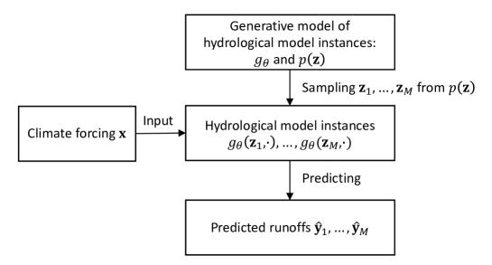
Essentially, and jointly define a generative model of hydrological model instances: by sampling values from , we can obtain hydrological model instances through . For a given climate forcing time series , these model instances produce the predicted runoff time series through . The processes for generating hydrological model instances and runoff predictions are illustrated in Figure 1.
2.2 Learning a generative model
Assume that for a catchment , we have , a set of pairs of climate forcing and runoff time series :
| (3) |
where is the index.
The machine learning task here is then to learn a general hydrological model and the latent vector value of the catchment from , such that the predicted runoff can closely match the observed runoff . Here, is a neural network parameterized by , and is a -dimensional numerical vector. For a given neural network structure and a value, the optimal values of and can be learned by solving the following optimization problem:
| (4) |
where is a loss function and is set to the root mean square error (RMSE) function in this study. The commonly used methods for training neural networks can generally be used to solve this problem, such as the backpropagation and stochastic decent algorithms [Goodfellow \BOthers. (\APACyear2016)]. The methods for determining the optimal network structure and are described in Section 2.4.
For the catchments in set , assuming that each catchment is associated with a climate forcing and runoff data set , the ”overall” optimal and values should then minimize the prediction errors for all the considered catchments, which can be derived by solving the following optimization problem:
| (5) |
This problem can also be solved using common neural network training algorithms. As shown in Figure 2, the and values are iteratively updated to minimize the runoff prediction errors until certain criteria is met. is then estimated from the learned values.
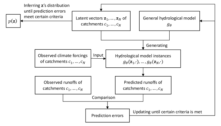
In this study, we assume that is an arbitrary probability density function that can be estimated directly from samples of , meaning that there are no constraints on the forms of . This is a simpler assumption compared to those used in some popular latent variable-based generative models, such as Variational Autoencoders [Kingma \BBA Welling (\APACyear2019)] and DeepSDF [Park \BOthers. (\APACyear2019)], which typically restrict to simple distribution functions (such as normal distributions) to allow for easy sampling of from latent space. In this study, a simpler assumption is used to clearly present the generative modeling approach. Also, no regularization terms are used in equations 4 and 5 to penalize high values of [Aggarwal (\APACyear2016)]. These simple treatments are shown to be sufficient for certain runoff prediction tasks in later sections of this paper.
2.3 Application and verification of a generative model
In general, once the value is learned, can be used much like a conventional lumped model class for discriminative modeling tasks. That is, requires only a few numerical values (i.e., the value) to generate a model instance, and these values can be optimized using the climate forcing and runoff data of a catchment. The resulting model instance can be thought of as a ”calibrated model” that can be reused to predict runoffs under different climate forcing conditions.
However, it is important to specify and test the assumptions involved in the generative modeling approach. There are two types of assumptions involved, one explicit and one implicit. The explicit assumption is that the runoff generation processes of a catchment can be sufficiently well characterized by a fixed numerical vector, where ”fixed” means that they are invariant under different climate forcing conditions. The implicit assumption is that for a ”new” catchment not used for learning the generative model, , there exists at least one vector in latent space that can characterize its runoff generation processes sufficiently well such that approximates the true runoff prediction function .
The explicit assumption is also used in many of the current hydrological modeling studies, where the calibrated model instances are used to predict runoffs under different climate forcing conditions. Therefore, testing methods used in these studies can be used here to test the explicit assumption. For example, the split-sample testing method can be used, which evaluates the usefulness of a calibrated model instance when applied to a period not used for model calibration (i.e., a test period).
The implicit assumption can be verified if we can learn a general hydrological model that is capable of accurately predicting the runoffs of an arbitrary catchment (that is not used in learning ), given an optimal estimated from ’s data. For a catchment , the optimal value of associated with it can be derived by solving the following optimization problem:
| (6) |
where is the available forcing and runoff data set of , and is a loss function. This optimization problem is very similar to the one defined in Equation 4. The only difference is that is a fixed value here instead of a decision variable. Since the dimension of (i.e., ) is low, this optimization problem can be solved using many general optimization algorithms that are commonly used in hydrology.
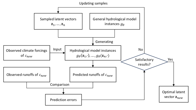
The process of finding the optimal value is illustrated in Figure 3, where candidate values are iteratively updated according to the prediction errors using a general optimization algorithm, and the optimization process is terminated when certain criteria are met. The overall process is again very similar to the process of learning a generative model (Figure 2), except that here is fixed and only the data from the catchment (instead of a collection of catchments) is used.
2.4 Architecture of a generative model and training strategy
The proposed generative model consists of two parts, and . can be represented by a neural network that takes two inputs, a latent vector and a multi-step and multi-dimensional climate forcing time series . is an arbitrary density function that is to be estimated from samples of values of different catchments (see Figure 2).
The architecture used in this study is shown in Figure 4, where an LSTM network [Gers \BOthers. (\APACyear2000)] parameterized by is used to transform and into . The LSTM network processes the input in a sequential manner. At each step, is concatenated with the climate forcing of that time step, which is then fed into the network. This simple concatenation operation is used to ensure that the inputs at different time steps are of the same dimension. For an introduction to LSTM in rainfall-runoff modeling, see \citeAKratzert2018. It is also possible to use other neural network architectures that are well suited for time series modeling, such as EA-LSTM [Kratzert, Klotz, Shalev\BCBL \BOthers. (\APACyear2019)], Transformers [Vaswani \BOthers. (\APACyear2017)], and Temporal Convolutional Networks (TCN; \citeABai2018).
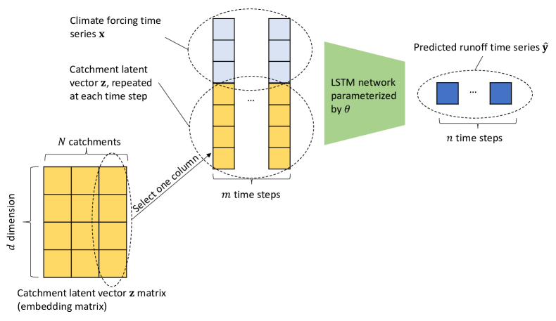
The latent vectors of a set of catchments can be effectively stored in an embedding matrix of size , where is latent dimension, as shown in Figure 4. To make runoff prediction for a given catchment , its associated is retrieved first from the embedding matrix using the index and then fed to the LSTM network. The embedding matrix can be considered as a simple look-up table storing numeric values. During training, the gradient of the loss function with respect to a value can be computed. This allows the embedding matrix to be learned together with using backpropagation algorithms.
There are several hyperparameters used in the model architecture shown in Figure 4, such as (i.e., the dimension of latent vector), the dimension of the hidden state, and the number of recurrent layers of the LSTM network. A number of hyperparameters are also used in the model training process, including batch size, number of epochs, and learning rate, and type of the optimizer. These hyperparameters should be set prior to training and can affect the quality of the learned model. The candidate value was 2, 4, 8, and 16, and the ranges of the other hyperparameters are listed in Table S1.
In this study, a Bayesian optimization algorithm implemented in the ”Optuna” Python library [Akiba \BOthers. (\APACyear2019)] was used to derive the optimal hyperparameters, which consists of the following steps. First, a training, validation, and test data set is created by extracting and combining the climate forcing and runoff time series of each catchment from their corresponding data sets . The Bayesian optimization algorithm is then applied to find the optimal values of the hyperparameters that minimize the runoff prediction error on the validation data set when learning and the embedding matrix (i.e., the values of catchments) on the training data set. The optimal hyperparameters are then applied to learn and the embedding matrix from the data set combining the training and validation sets, and the resulting generative model is then tested on the test data set to estimate the generalization error [Cawley \BBA Talbot (\APACyear2010)]. Finally, all available data is used to train a final generative model using the optimal hyperparameters. See Table S1 for the hyperparameter values used for the Bayesian optimization algorithm.
2.5 Genetic algorithms for optimizing latent vector values of new catchments
As discussed in Section 2.3, the optimal latent vector value of a new catchment can be derived using a generic model calibration algorithm. This study used a simple genetic algorithm (GA) implemented in the ”PyGAD” Python library [Gad (\APACyear2021)]. The optimal of a catchment minimizes the runoff prediction error on the calibration data set. In this study, we did not further split the calibration data set for optimizing the hyperparameters used in the GA, such as the number of generations, in order to obtain a baseline performance value (instead of a higher benchmark) and to demonstrate the effectiveness of the generative modeling approach. The hyperparameter values used are shown in Table S1. An introduction to GA is omitted here and can be found in \citeALuke2013.
2.6 Climate forcing and runoff data sets used in numerical experiments
Three data sets covering catchments from different parts of the world were used in this study. They are CAMELS (Catchment Attributes and Meteorology for Large-sample Studies; \citeANewman2014_data,Newman2015,Addor2017), CAMELS-CH (Catchment Attributes and MEteorology for large-sample Studies - Switzerland; \citeAHoge2023), and Caravan [Kratzert \BOthers. (\APACyear2023)]. CAMELS, CAMELS-CH, and Caravan include catchments mainly from the US, Switzerland and neighboring countries, and around the world, respectively. A number of catchments were selected from each data set based on their location and data availability, as shown in Table 1. Catchment mean daily precipitation (P), temperature (T), and potential evapotranspiration (PET) were used as the climate forcing variables in this study because of their common use in many conventional lump models [Knoben, Freer, Fowler\BCBL \BOthers. (\APACyear2019)], and daily runoff (Q) was used as the prediction target. These four variables were available in the Caravan and CAMELS-CH data sets and were extracted and derived from the CAMELS data set processed by \citeAKnoben2020.
| Data set |
|
Splits of the data set | Selection criteria | |||||||||||
|---|---|---|---|---|---|---|---|---|---|---|---|---|---|---|
| Caravan | 3007 |
|
|
|||||||||||
|
559 |
|
|
|||||||||||
|
157 |
|
|
As shown in Table 1, each data set is divided into a number of smaller subsets according to their role in the numerical experiments. For the Caravan data set, three subsets were created, and they were used to train and test generative models using the methods described in Section 2.4. Both the CAMELS and CAMELS-CH data sets were split into two subsets: a calibration and a test set. The catchments in the two data sets were considered as ”new” catchments, for which the optimal values were derived and tested with the calibration and test sets using the methods described in Section 2.5.
2.7 Benchmark data on lumped hydrological models’ performance
Knoben2020 calibrated 36 lumped hydrological model classes for 559 catchments from the CAMELS data set. These model classes include Xinanjiang Model, TOPMODEL, HBV-96, VIC, and GR4J. They reported the runoff prediction accuracies of the calibrated model instances, as measured by the KGE (Kling-Gupta efficiency) criterion [Gupta \BOthers. (\APACyear2009)]. More details of the model performance data set can be found in \citeAKnoben2020. These values were used in this study as benchmarks for evaluating the usefulness of the generative models in runoff prediction tasks.
3 Numerical experiments and results
In the numerical experiments, we trained generative models (i.e., combinations of and ) using the Caravan data set. Then, the generative models were tested on the CAMELS and CAMELS-CH data sets in terms of their ability to perform discriminative tasks (i.e., modeling runoffs for ”new” catchments). Finally, we evaluate the effect of latent vector values on the predicted hydrographs.
3.1 Using generative models in regional hydrological modeling
3.1.1 Experiments performed
In the first experiment, we used the methods described in Section 2.4 to train a general hydrological model using the training and validation sets of Caravan. The final model was trained on the combination of the two sets, and the optimal hyperparameters used during training were obtained by minimizing the prediction errors on the validation set when training on the training set. Each of the 3,007 selected Caravan catchments was assigned a latent vector . Thus, a model instance was derived for each . The model instances were tested on the test set using the KGE criterion. The purpose of this experiment is to evaluate the usefulness of the generative modeling approach in a regional modeling setting, where the model instances were jointly learned from data for multiple catchments.
The input climate forcing time series to each model instance is a two-year (i.e., 730 days) P, T, and PET time series, and the prediction target associated with a sample of is the second year (i.e., from day 366 to day 730) Q time series. Thus, the assumption used here is that the runoff depth of a catchment observed on a particular day is predictable by the one-year climate conditions that preceded that day.
When training (i.e. updating the values of ), the and pairs of each were randomly sampled from the specified period of different sets (as listed in Table 1). During validation and test (i.e., when is fixed), the and samples were taken regularly from the specified period with an interval of one year, which ensures that the runoff time series can be predicted for the entire validation or testing period.
3.1.2 Results
Using Bayesian optimization, we found that the optimal value of (i.e., the latent vector dimension) was 8. For each of the 3,007 caravan catchments , an 8-dimensional latent vector was learned, corresponding to a concrete model instance. The non-exceedance probability of the KGE score of the model instances computed for the training and test periods is shown in Figure 5. The two non-exceedance probability curves show that the model instances generally had higher prediction accuracies during the training period than during the test period. Note that the training period here includes the periods specified by both the training and validation sets of Caravan.
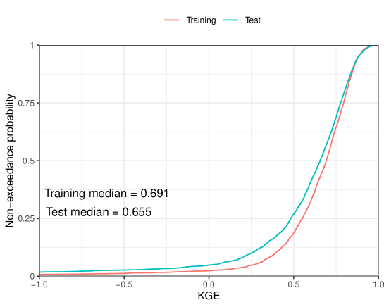
The median KGE of the training and test periods is 0.691 and 0.655, respectively. This result indicates that the prediction accuracy was generally acceptable for more than 50% of the catchments, although performance gaps between the training and test periods can be observed.
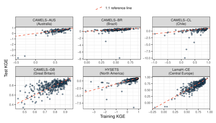
The Caravan data set contains the forcing and runoff data of catchments of different countries or regions [Kratzert \BOthers. (\APACyear2023)]. The runoff data of Caravan were aggregated from several existing open data sets. Figure 6 thus compares the training and test KEG scores of model instances of catchments of different countries or regions. The training and test KGE scores are positively correlated for all countries or regions considered. For the catchments of the Great Britain and the Central Europe regions, both the training and the test KGE scores are generally higher than 0. However, in the other regions, as indicated by the few large negative KGE scores, some model instances have poor performance.
3.1.3 Discussions
The test KGE results shown in Figures 5 and 6 indicate that the generative model learned from climate forcing and runoff data alone was generally useful in a regional modeling setting, at least for some catchments. Unlike most current regional modeling studies, no catchment attributes were used. The proposed generative modeling approach does not assume any correlation between catchment attributes and hydrological functions. It simply aims to learn a set of model instances (i.e., numerical functions) that can accurately reproduce the observed hydrographs without constraining the value of the catchment latent vectors. Future studies can thus explore how to incorporate catchment attributes and other physically meaningful information into the generative modeling framework to ensure that the learned model instances have certain desirable properties.
The optimal number of latent dimensions was found to be 8, implying that the differences between the hydrological behavioral characteristics of different catchments can be well described using a small number of numerical values. This result is consistent with the findings in \citeAYang2023 that the degree of fit between a catchment and a model instance can be sufficiently well explained by a small number of factors. However, the exact information encoded in each dimension is unknown. In contrast, the physical meaning of the parameters that are used in the conventional lumped model classes is known. In Section 3.3, the effect of latent vector values on the predicted hydrographs is examined.
Similar to the traditional lumped model classes, the generative model is also not immune to the overfitting problem, as indicated by the performance gap between the training and test KGE scores shown in Figures 5. The overfitting could be caused by the catchments having different runoff generation patterns during the training and test periods, and the model instances having learned ”noise” in the forcing and runoff time series in addition to the true patterns. The problem associated with shifting runoff generation patterns may be mitigated by treating the catchment runoff function and the catchment latent vector as functions of time, rather than assuming that they are fixed in Equation 2. And the problems of learning noise from data may be mitigated by the use of different machine learning architectures, regularization methods, and more training data. Since our goal is to provide a simple introduction to the generative modeling approach, these options were not explored in this study. In addition, the factors that contribute to the differences in the predictive performance across catchments were not investigated in this study.
3.2 Using generative models as conventional lumped model classes
3.2.1 Experiments performed
In the second experiment, we evaluated the usefulness of a generative model trained on data from a set of catchments in modeling ”new” catchments outside the catchment set. The generative model used in the experiment was trained on the entire Caravan data set using the hyperparameters obtained in Section 3.1. The optimal latent vector values of the CAMELS and CAMELS-CH catchments were derived using the optimization method described in Section 2.5 with the calibration period data. The range of each dimension of was determined based on the minimum and maximum values of that dimension of the values derived for the catchments in the training data set. The resulting model instances, i.e., associated with different catchments, were then tested on the test period data. The predictive performance of the CAMELS catchment model instances was then compared with that obtained for the conventional lumped model classes in \citeAKnoben2020.
3.2.2 Results
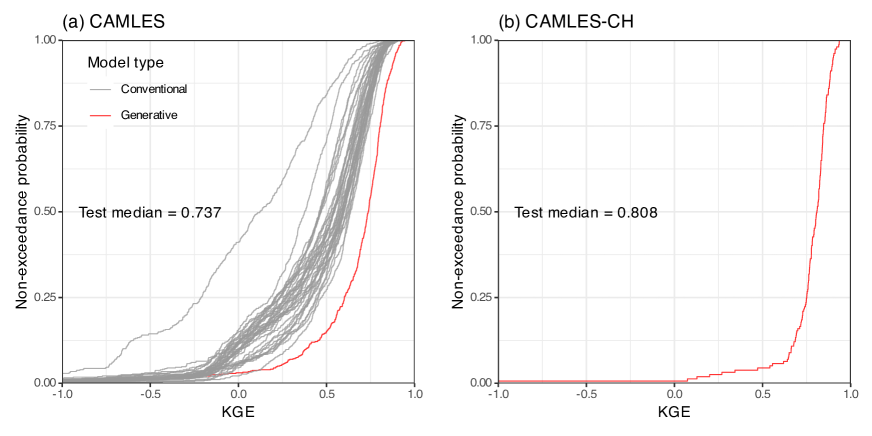
The predictive performance of the model instances derived by optimizing the latent vector values is shown in Figure 7. The median test KGE scores were 0.737 and 0.808 for the CAMELS and CAMELS-CH catchments, respectively. The median KGE score of the CAMELS catchments was comparable to previous deep learning studies that learned model instances directly from the data, e.g., \citeABotterill2023 and \citeALi2022. Figure 7a also compares the performances of the model instances created using the generative model and 36 conventional lumped model classes. With the exception of the bottom 10% of model instances, the generative model-based model instances generally performed better than those derived from any of the lumped model classes.
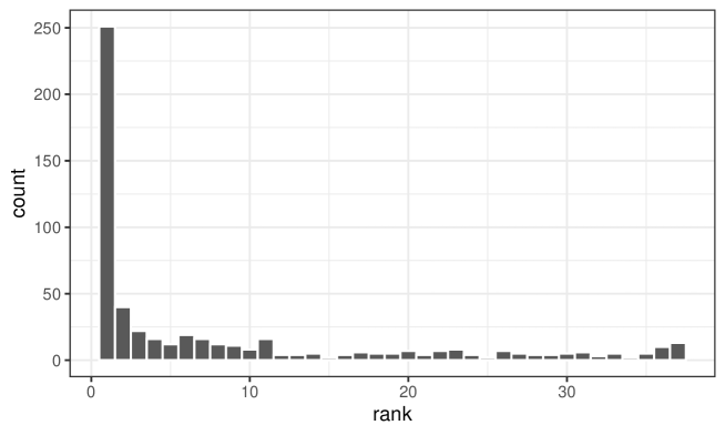
The performance of the generative model based-instances of the CAMELS catchments was compared to their counterparts derived using the conventional lumped model classes, and their ranking is shown in Figure 8. The generative model-based instances ranked in the top 1, top 3, and top 10 for 44.9%, 56.0%, and 72.8% of the catchments, respectively. However, these models can have very low rankings in some catchments.
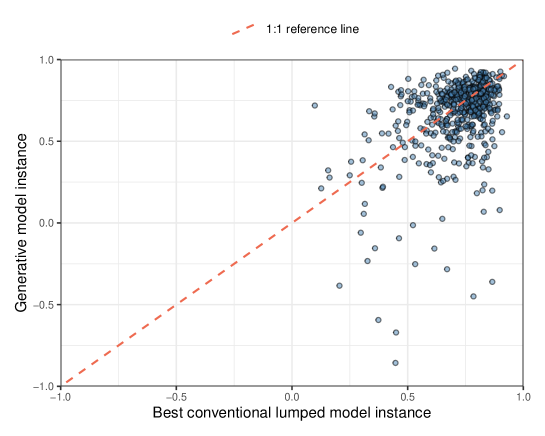
The generative model-based instance of each CAMELS catchment was compared to the best of the 36 corresponding lumped model instances in Figure 9. A weak to moderate positive correlation (Pearson correlation coefficient ) can be observed between the KGE scores of the two sets of model instances. In some catchments, the generative model-based instances performed significantly worse than the best lumped model instances, as indicated by the negative KGE values. The KGE values of the best lumped model instances were rarely negative.
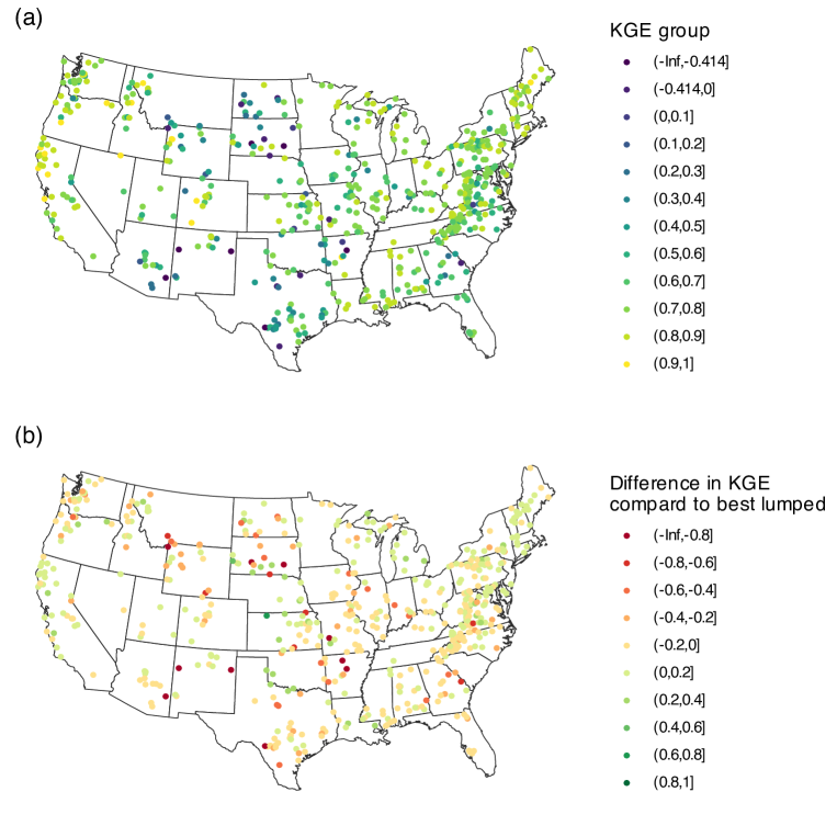
The spatial distribution pattern of the test KGE score of the generative model-based instances is shown in Figure 10a. The model instances of the catchments in the Pacific Mountain Systems and Appalachian Highlands regions (i.e., the west and east coasts of the US) generally have good predictive performance. \citeAKnoben2019b showed that when mean streamflow is used as a predictor, and catchments with were mostly found in the Interior Plains, Rocky Mountain System, and Intermontane Plateaus (i.e., central and western US). The spatial distribution pattern of the difference between the generative model-based instances and the best lumped model instances, in terms of the test KGE value, is shown in Figure 10b. The result shows that these two sets of model instances generally had comparable performance in the Pacific Mountain Systems and Appalachian Highlands regions, and in the other regions the generative model-based instances could perform significantly worse.
3.2.3 Discussions
The experimental results show that it is possible to learn a generative model of hydrological model instances directly from data such that, by sampling from its parameter space (i.e., latent vector space), model instances that resemble real-world catchments can be produced. Unlike conventional lumped model classes, the generative models are automatically learned from data without the use of specific hydrological knowledge. Thus, this study proposes a purely data-driven approach to easily generate meaningful hydrological model instances. Note that in contrast to many current studies, no catchment attributes are required to generate a model instance.
The model instances generated by the generative model were found to have comparable performance to those learned directly from the data using deep learning methods (i.e., the discriminative modeling approach), but with much less effort. To create a model instance for a catchment, the generative modeling approach requires only the estimation of a few parameters using a generic model calibration algorithm, while the discriminative modeling approach requires the learning of many more parameters (e.g., tens of thousands). Given a limited amount of data, reducing the number of trainable parameters in a numerical model may alleviate the overfitting problem. However, a formal verification of this assumption is needed.
In comparison to the 36 conventional lumped model classes, the generative model showed comparable or better ability to model the runoff generation process in the majority of the CAMELS catchments. Therefore, the generative models can be a useful addition to a modeler’s lumped modeling toolbox. The better performance of the machine learning models in some catchments indicates that our hydrological knowledge (used to develop lumped model classes) was insufficient, which is similar to the conclusions of other machine learning research in hydrological modeling. However, it should be noted that the generative model can have poor performance in some catchments where the conventional lumped models can have good performance. The poor performance may be explained by that the training data set does not contain catchments with similar runoff generation characteristics, or that the ability of the generative model to extrapolate different runoff generation functions is limited. Future studies can therefore use a larger or more diverse data set for training of a generative model and then test whether this model has a broader applicability.
The comparison between the best lumped model and the generative model also shows that a collection of conventional lumped models can provide competitive results compared to the models derived using modern data-driven approaches. And the lower bound of their performance is much higher than that of the data-driven models. Thus, we argue that lumped models are still very useful for hydrological prediction tasks. The effectiveness of the lumped and data-driven models in hydrological prediction under different conditions should be rigorously tested using different methods, including metamorphic testing [Yang \BBA Chui (\APACyear2021)] and interpretable machine learning methods [Molnar (\APACyear2022)].
3.3 Effect of latent vector value on predicted runoff hydrograph
3.3.1 Experiments performed
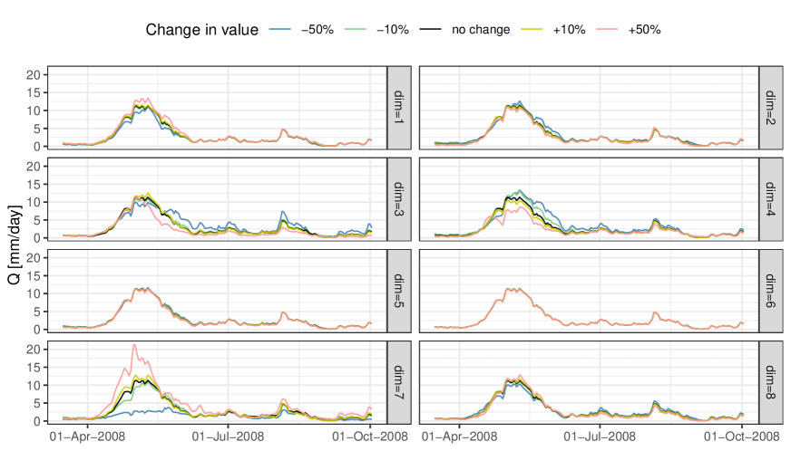
The purpose of this experiment is to investigate how the value of each dimension of the latent vector affects the predicted hydrograph. We chose a random catchment from the CAMELS data set, the Fish River catchment near Fort Kent, Maine (USGS 01013500). The model instance associated with the catchment was developed in Section 3.2, which was derived by optimizing the 8-dimensional latent vector to minimize prediction errors during the calibration period. We selected a period with the highest predicted runoff peak and then varied the value of each dimension of the latent vector by -50%, -10%, +10%, and +50% to investigate how the predicted hydrograph changed.
3.3.2 Results
The hydrographs corresponding to different latent vector values are shown in Figure 11. The predicted hydrograph was found to be sensitive to the values of a few selected dimensions, such as the 3rd, 4th, and 7th dimensions. Changing the values of different dimensions can have different effects on the predicted hydrograph. For example, the predicted peak runoff increased when increasing the value of the 7th dimension; changing the value of the 3rd dimension changed the predicted recession limps and low flows. In general, the amount of change in the predicted hydrograph was found to be positively correlated with changes in the value of a particular dimension, such that a +50% change in latent vector value can cause a greater change in the predicted hydrograph than a +10% change.
3.3.3 Discussions
The experimental result shows that latent vector values can encode information that reflects certain hydrological behavioral characteristics of a catchment, such as how quickly runoff declines after peak runoff during a flood event. However, it can be difficult to determine the exact information encoded by each dimension. This is because a dimension can encode different information when the input forcing varies and when the latent vectors are at different locations in the latent space. The latent vector values may be more easily interpreted if certain constraints can be imposed on the latent vectors when training the model. For example, forcing each dimension to be independent of the other allows for a more straightforward analysis of each individual dimension. The sensitivity analysis methods currently used in hydrology [X. Song \BOthers. (\APACyear2015)] may also be useful in studying how the latent vector value affects the predicted hydrograph.
Unlike conventional lumped model classes, the ”meaning” of each parameter (i.e., each dimension of the latent vector) is automatically learned from the data, rather than being predefined. It is interesting to evaluate whether the optimal latent vector of a catchment can be predicted by its physical properties. If this is the case, then a reasonable model instance can be generated for an ungauged catchment using the generative model and the physical properties of the catchment. The optimal latent vectors of different catchments may also be useful for catchment classification and catchment similarity analysis research. Further research on these topics is recommended.
4 Conclusions
This study presents a generative modeling approach to rainfall-runoff modeling. The generative models, which are automatically learned from the climate forcing and runoff data from a set of catchments, are capable of producing hydrological model instances (i.e., functions that predict runoffs based on climate forcing) that closely resemble real-world catchments. A model instance can be easily produced by providing the generative model with a numerical vector sampled from a relatively low-dimensional (i.e., 8-dimensional) space. For a given catchment, a well-fitting model instance capable of making accurate runoff predictions can be derived by searching through the parameter space using a generic model calibration algorithm. That is, a generative model can be used similarity as a conventional lumped hydrological model structure, that an optimal model instance for a catchment can be found through model calibration.
The generative models developed in this study were found to be capable of producing well-fitting model instances for catchments worldwide. For an arbitrary catchment not used to train the generative model, optimal model instances derived using a generic model calibration algorithm were found to be able to provide prediction accuracies comparable to or better than the conventional lumped model classes. These results suggest that it is possible to derive useful hydrological model structures from data without reliance on human knowledge of catchment-scale physical processes.
This study also shows that the hydrological behavior of catchments worldwide can be sufficiently well characterized by a small number of factors, i.e. a latent vector. The optimal value of these factors of a catchment can be estimated from the climate forcing and runoff time series alone, without applying any specific hydrological knowledge or referring to any catchment attributes (that describe the physical properties of the catchments). The low-dimensional representation of the catchment hydrological function can be useful for catchment similarity analysis and catchment clustering. However, the exact meaning of these factors is currently unknown, and future studies aimed at interpreting the learned factors are recommended.
Acknowledgements.
The LaTex template used to create this file is from the AGU Geophysical Research Letters AGUTeX Article https://www.overleaf.com/latex/templates/agu-geophysical-research-letters-agutex-article/rnyzczmyvkbj. We thank Wouter Knoben for sharing the processed CAMELS forcing data used in \citeAKnoben2020 and commenting on the paper. The source code used in this research can be found in https://github.com/stsfk/deep_lumped.References
- Addor \BOthers. (\APACyear2017) \APACinsertmetastarAddor2017{APACrefauthors}Addor, N., Newman, A\BPBIJ., Mizukami, N.\BCBL \BBA Clark, M\BPBIP. \APACrefYearMonthDay2017. \BBOQ\APACrefatitleThe CAMELS data set: catchment attributes and meteorology for large-sample studies The camels data set: catchment attributes and meteorology for large-sample studies.\BBCQ \APACjournalVolNumPagesHydrology and Earth System Sciences21105293–5313. {APACrefURL} https://hess.copernicus.org/articles/21/5293/2017/ {APACrefDOI} 10.5194/hess-21-5293-2017 \PrintBackRefs\CurrentBib
- Aggarwal (\APACyear2016) \APACinsertmetastarAggarwal2016{APACrefauthors}Aggarwal, C\BPBIC. \APACrefYear2016. \APACrefbtitleRecommender Systems: The Textbook Recommender systems: The textbook. \APACaddressPublisherSpringer. \PrintBackRefs\CurrentBib
- Akiba \BOthers. (\APACyear2019) \APACinsertmetastarAkiba2019{APACrefauthors}Akiba, T., Sano, S., Yanase, T., Ohta, T.\BCBL \BBA Koyama, M. \APACrefYearMonthDay2019. \APACrefbtitleOptuna: A Next-generation Hyperparameter Optimization Framework. Optuna: A next-generation hyperparameter optimization framework. \PrintBackRefs\CurrentBib
- M\BPBIP. Anderson \BOthers. (\APACyear2015) \APACinsertmetastarAnderson2015{APACrefauthors}Anderson, M\BPBIP., Woessner, W\BPBIW.\BCBL \BBA Hunt, R\BPBIJ. \APACrefYearMonthDay2015. \BBOQ\APACrefatitleChapter 6 - More on Sources and Sinks Chapter 6 - more on sources and sinks.\BBCQ \BIn M\BPBIP. Anderson, W\BPBIW. Woessner\BCBL \BBA R\BPBIJ. Hunt (\BEDS), \APACrefbtitleApplied Groundwater Modeling (Second Edition) Applied groundwater modeling (second edition) (\PrintOrdinalSecond Edition \BEd, \BPG 257-301). \APACaddressPublisherSan DiegoAcademic Press. \PrintBackRefs\CurrentBib
- S. Anderson \BBA Radić (\APACyear2022) \APACinsertmetastarAnderson2022{APACrefauthors}Anderson, S.\BCBT \BBA Radić, V. \APACrefYearMonthDay2022. \BBOQ\APACrefatitleEvaluation and interpretation of convolutional long short-term memory networks for regional hydrological modelling Evaluation and interpretation of convolutional long short-term memory networks for regional hydrological modelling.\BBCQ \APACjournalVolNumPagesHydrology and Earth System Sciences263795–825. \PrintBackRefs\CurrentBib
- Bai \BOthers. (\APACyear2018) \APACinsertmetastarBai2018{APACrefauthors}Bai, S., Kolter, J\BPBIZ.\BCBL \BBA Koltun, V. \APACrefYearMonthDay2018. \APACrefbtitleAn Empirical Evaluation of Generic Convolutional and Recurrent Networks for Sequence Modeling. An empirical evaluation of generic convolutional and recurrent networks for sequence modeling. \PrintBackRefs\CurrentBib
- Beven (\APACyear2011) \APACinsertmetastarBeven2011{APACrefauthors}Beven, K. \APACrefYear2011. \APACrefbtitleRainfall-Runoff Modelling: The Primer Rainfall-runoff modelling: The primer. \APACaddressPublisherWiley. {APACrefURL} https://books.google.com.hk/books?id=eI-jjlTirlAC \PrintBackRefs\CurrentBib
- Black (\APACyear1997) \APACinsertmetastarBlack1997{APACrefauthors}Black, P\BPBIE. \APACrefYearMonthDay1997. \BBOQ\APACrefatitleWATERSHED FUNCTIONS1 Watershed functions1.\BBCQ \APACjournalVolNumPagesJAWRA Journal of the American Water Resources Association3311-11. {APACrefURL} https://onlinelibrary.wiley.com/doi/abs/10.1111/j.1752-1688.1997.tb04077.x {APACrefDOI} https://doi.org/10.1111/j.1752-1688.1997.tb04077.x \PrintBackRefs\CurrentBib
- Botterill \BBA McMillan (\APACyear2023) \APACinsertmetastarBotterill2023{APACrefauthors}Botterill, T\BPBIE.\BCBT \BBA McMillan, H\BPBIK. \APACrefYearMonthDay20233. \BBOQ\APACrefatitleUsing Machine Learning to Identify Hydrologic Signatures With an Encoder–Decoder Framework Using machine learning to identify hydrologic signatures with an encoder–decoder framework.\BBCQ \APACjournalVolNumPagesWater Resources Research59e2022WR033091. {APACrefURL} https://onlinelibrary.wiley.com/doi/full/10.1029/2022WR033091 {APACrefDOI} 10.1029/2022WR033091 \PrintBackRefs\CurrentBib
- Cawley \BBA Talbot (\APACyear2010) \APACinsertmetastarCawley2010{APACrefauthors}Cawley, G\BPBIC.\BCBT \BBA Talbot, N\BPBIL. \APACrefYearMonthDay2010. \BBOQ\APACrefatitleOn over-fitting in model selection and subsequent selection bias in performance evaluation On over-fitting in model selection and subsequent selection bias in performance evaluation.\BBCQ \APACjournalVolNumPagesThe Journal of Machine Learning Research112079–2107. \PrintBackRefs\CurrentBib
- Coron \BOthers. (\APACyear2017) \APACinsertmetastarCoron2017{APACrefauthors}Coron, L., Thirel, G., Delaigue, O., Perrin, C.\BCBL \BBA Andréassian, V. \APACrefYearMonthDay2017. \BBOQ\APACrefatitleThe suite of lumped GR hydrological models in an R package The suite of lumped gr hydrological models in an r package.\BBCQ \APACjournalVolNumPagesEnvironmental Modelling & Software94166-171. \PrintBackRefs\CurrentBib
- Efstratiadis \BBA Koutsoyiannis (\APACyear2010) \APACinsertmetastarEfstratiadis2010{APACrefauthors}Efstratiadis, A.\BCBT \BBA Koutsoyiannis, D. \APACrefYearMonthDay2010. \BBOQ\APACrefatitleOne decade of multi-objective calibration approaches in hydrological modelling: a review One decade of multi-objective calibration approaches in hydrological modelling: a review.\BBCQ \APACjournalVolNumPagesHydrological Sciences Journal–Journal Des Sciences Hydrologiques55158–78. \PrintBackRefs\CurrentBib
- Feng \BOthers. (\APACyear2020) \APACinsertmetastarFeng2020{APACrefauthors}Feng, D., Fang, K.\BCBL \BBA Shen, C. \APACrefYearMonthDay2020. \BBOQ\APACrefatitleEnhancing Streamflow Forecast and Extracting Insights Using Long-Short Term Memory Networks With Data Integration at Continental Scales Enhancing streamflow forecast and extracting insights using long-short term memory networks with data integration at continental scales.\BBCQ \APACjournalVolNumPagesWater Resources Research569e2019WR026793. {APACrefURL} https://agupubs.onlinelibrary.wiley.com/doi/abs/10.1029/2019WR026793 \APACrefnotee2019WR026793 2019WR026793 {APACrefDOI} https://doi.org/10.1029/2019WR026793 \PrintBackRefs\CurrentBib
- Foster (\APACyear2022) \APACinsertmetastarFoster2022{APACrefauthors}Foster, D. \APACrefYear2022. \APACrefbtitleGenerative Deep Learning Generative deep learning. \APACaddressPublisherO’Reilly Media. \PrintBackRefs\CurrentBib
- Gad (\APACyear2021) \APACinsertmetastarGad2021{APACrefauthors}Gad, A\BPBIF. \APACrefYearMonthDay2021. \APACrefbtitlePyGAD: An Intuitive Genetic Algorithm Python Library. Pygad: An intuitive genetic algorithm python library. \PrintBackRefs\CurrentBib
- Gers \BOthers. (\APACyear2000) \APACinsertmetastarGers2000{APACrefauthors}Gers, F\BPBIA., Schmidhuber, J.\BCBL \BBA Cummins, F. \APACrefYearMonthDay2000. \BBOQ\APACrefatitleLearning to forget: Continual prediction with LSTM Learning to forget: Continual prediction with lstm.\BBCQ \APACjournalVolNumPagesNeural computation12102451–2471. \PrintBackRefs\CurrentBib
- Goodfellow \BOthers. (\APACyear2016) \APACinsertmetastarGoodfellow2016{APACrefauthors}Goodfellow, I., Bengio, Y.\BCBL \BBA Courville, A. \APACrefYear2016. \APACrefbtitleDeep learning Deep learning. \APACaddressPublisherMIT press. \PrintBackRefs\CurrentBib
- Gupta \BOthers. (\APACyear2009) \APACinsertmetastarGupta2009{APACrefauthors}Gupta, H\BPBIV., Kling, H., Yilmaz, K\BPBIK.\BCBL \BBA Martinez, G\BPBIF. \APACrefYearMonthDay2009. \BBOQ\APACrefatitleDecomposition of the mean squared error and NSE performance criteria: Implications for improving hydrological modelling Decomposition of the mean squared error and nse performance criteria: Implications for improving hydrological modelling.\BBCQ \APACjournalVolNumPagesJournal of Hydrology377180-91. {APACrefURL} https://www.sciencedirect.com/science/article/pii/S0022169409004843 {APACrefDOI} https://doi.org/10.1016/j.jhydrol.2009.08.003 \PrintBackRefs\CurrentBib
- Höge \BOthers. (\APACyear2023) \APACinsertmetastarHoge2023{APACrefauthors}Höge, M., Kauzlaric, M., Siber, R., Schönenberger, U., Horton, P., Schwanbeck, J.\BDBLFenicia, F. \APACrefYearMonthDay2023. \BBOQ\APACrefatitleCAMELS-CH: hydro-meteorological time series and landscape attributes for 331 catchments in hydrologic Switzerland Camels-ch: hydro-meteorological time series and landscape attributes for 331 catchments in hydrologic switzerland.\BBCQ \APACjournalVolNumPagesEarth System Science Data Discussions20231–46. \PrintBackRefs\CurrentBib
- Kingma \BBA Welling (\APACyear2019) \APACinsertmetastarKingma2019{APACrefauthors}Kingma, D\BPBIP.\BCBT \BBA Welling, M. \APACrefYearMonthDay2019. \BBOQ\APACrefatitleAn Introduction to Variational Autoencoders An introduction to variational autoencoders.\BBCQ \APACjournalVolNumPagesFoundations and Trends® in Machine Learning124307–392. {APACrefURL} https://doi.org/10.1561%2F2200000056 {APACrefDOI} 10.1561/2200000056 \PrintBackRefs\CurrentBib
- Knoben, Freer, Fowler\BCBL \BOthers. (\APACyear2019) \APACinsertmetastarKnoben2019{APACrefauthors}Knoben, W\BPBIJ\BPBIM., Freer, J\BPBIE., Fowler, K\BPBIJ\BPBIA., Peel, M\BPBIC.\BCBL \BBA Woods, R\BPBIA. \APACrefYearMonthDay2019. \BBOQ\APACrefatitleModular Assessment of Rainfall–Runoff Models Toolbox (MARRMoT) v1.2: an open-source, extendable framework providing implementations of 46 conceptual hydrologic models as continuous state-space formulations Modular assessment of rainfall–runoff models toolbox (marrmot) v1.2: an open-source, extendable framework providing implementations of 46 conceptual hydrologic models as continuous state-space formulations.\BBCQ \APACjournalVolNumPagesGeoscientific Model Development1262463–2480. \PrintBackRefs\CurrentBib
- Knoben \BOthers. (\APACyear2020) \APACinsertmetastarKnoben2020{APACrefauthors}Knoben, W\BPBIJ\BPBIM., Freer, J\BPBIE., Peel, M\BPBIC., Fowler, K\BPBIJ\BPBIA.\BCBL \BBA Woods, R\BPBIA. \APACrefYearMonthDay2020. \BBOQ\APACrefatitleA Brief Analysis of Conceptual Model Structure Uncertainty Using 36 Models and 559 Catchments A brief analysis of conceptual model structure uncertainty using 36 models and 559 catchments.\BBCQ \APACjournalVolNumPagesWater Resources Research569e2019WR025975. {APACrefURL} https://agupubs.onlinelibrary.wiley.com/doi/abs/10.1029/2019WR025975 \APACrefnotee2019WR025975 10.1029/2019WR025975 {APACrefDOI} https://doi.org/10.1029/2019WR025975 \PrintBackRefs\CurrentBib
- Knoben, Freer\BCBL \BBA Woods (\APACyear2019) \APACinsertmetastarKnoben2019b{APACrefauthors}Knoben, W\BPBIJ\BPBIM., Freer, J\BPBIE.\BCBL \BBA Woods, R\BPBIA. \APACrefYearMonthDay2019. \BBOQ\APACrefatitleTechnical note: Inherent benchmark or not? Comparing Nash–Sutcliffe and Kling–Gupta efficiency scores Technical note: Inherent benchmark or not? comparing nash–sutcliffe and kling–gupta efficiency scores.\BBCQ \APACjournalVolNumPagesHydrology and Earth System Sciences23104323–4331. \PrintBackRefs\CurrentBib
- Kratzert \BOthers. (\APACyear2018) \APACinsertmetastarKratzert2018{APACrefauthors}Kratzert, F., Klotz, D., Brenner, C., Schulz, K.\BCBL \BBA Herrnegger, M. \APACrefYearMonthDay2018. \BBOQ\APACrefatitleRainfall–runoff modelling using Long Short-Term Memory (LSTM) networks Rainfall–runoff modelling using long short-term memory (lstm) networks.\BBCQ \APACjournalVolNumPagesHydrology and Earth System Sciences22116005–6022. \PrintBackRefs\CurrentBib
- Kratzert, Klotz, Herrnegger\BCBL \BOthers. (\APACyear2019) \APACinsertmetastarKratzert2019b{APACrefauthors}Kratzert, F., Klotz, D., Herrnegger, M., Sampson, A\BPBIK., Hochreiter, S.\BCBL \BBA Nearing, G\BPBIS. \APACrefYearMonthDay2019. \BBOQ\APACrefatitleToward Improved Predictions in Ungauged Basins: Exploiting the Power of Machine Learning Toward improved predictions in ungauged basins: Exploiting the power of machine learning.\BBCQ \APACjournalVolNumPagesWater Resources Research551211344-11354. {APACrefURL} https://agupubs.onlinelibrary.wiley.com/doi/abs/10.1029/2019WR026065 {APACrefDOI} https://doi.org/10.1029/2019WR026065 \PrintBackRefs\CurrentBib
- Kratzert, Klotz, Shalev\BCBL \BOthers. (\APACyear2019) \APACinsertmetastarKratzert2019a{APACrefauthors}Kratzert, F., Klotz, D., Shalev, G., Klambauer, G., Hochreiter, S.\BCBL \BBA Nearing, G. \APACrefYearMonthDay2019. \BBOQ\APACrefatitleTowards learning universal, regional, and local hydrological behaviors via machine learning applied to large-sample datasets Towards learning universal, regional, and local hydrological behaviors via machine learning applied to large-sample datasets.\BBCQ \APACjournalVolNumPagesHydrology and Earth System Sciences23125089–5110. \PrintBackRefs\CurrentBib
- Kratzert \BOthers. (\APACyear2023) \APACinsertmetastarKratzert2023{APACrefauthors}Kratzert, F., Nearing, G., Addor, N., Erickson, T., Gauch, M., Gilon, O.\BDBLMatias, Y. \APACrefYearMonthDay2023. \BBOQ\APACrefatitleCaravan - A global community dataset for large-sample hydrology Caravan - a global community dataset for large-sample hydrology.\BBCQ \APACjournalVolNumPagesScientific Data10161. \PrintBackRefs\CurrentBib
- Li \BOthers. (\APACyear2022) \APACinsertmetastarLi2022{APACrefauthors}Li, X., Khandelwal, A., Jia, X., Cutler, K., Ghosh, R., Renganathan, A.\BDBLKumar, V. \APACrefYearMonthDay2022. \BBOQ\APACrefatitleRegionalization in a Global Hydrologic Deep Learning Model: From Physical Descriptors to Random Vectors Regionalization in a global hydrologic deep learning model: From physical descriptors to random vectors.\BBCQ \APACjournalVolNumPagesWater Resources Research588e2021WR031794. {APACrefURL} https://agupubs.onlinelibrary.wiley.com/doi/abs/10.1029/2021WR031794 \APACrefnotee2021WR031794 2021WR031794 {APACrefDOI} https://doi.org/10.1029/2021WR031794 \PrintBackRefs\CurrentBib
- Luke (\APACyear2013) \APACinsertmetastarLuke2013{APACrefauthors}Luke, S. \APACrefYear2013. \APACrefbtitleEssentials of Metaheuristics Essentials of metaheuristics (\PrintOrdinalsecond \BEd). \APACaddressPublisherLulu. \APACrefnoteAvailable for free at http://cs.gmu.edu/sean/book/metaheuristics/ \PrintBackRefs\CurrentBib
- Ma \BOthers. (\APACyear2021) \APACinsertmetastarMa2021{APACrefauthors}Ma, K., Feng, D., Lawson, K., Tsai, W\BHBIP., Liang, C., Huang, X.\BDBLShen, C. \APACrefYearMonthDay2021. \BBOQ\APACrefatitleTransferring Hydrologic Data Across Continents – Leveraging Data-Rich Regions to Improve Hydrologic Prediction in Data-Sparse Regions Transferring hydrologic data across continents – leveraging data-rich regions to improve hydrologic prediction in data-sparse regions.\BBCQ \APACjournalVolNumPagesWater Resources Research575e2020WR028600. {APACrefURL} https://agupubs.onlinelibrary.wiley.com/doi/abs/10.1029/2020WR028600 \APACrefnotee2020WR028600 2020WR028600 {APACrefDOI} https://doi.org/10.1029/2020WR028600 \PrintBackRefs\CurrentBib
- Makhzani \BOthers. (\APACyear2015) \APACinsertmetastarMakhzani2015{APACrefauthors}Makhzani, A., Shlens, J., Jaitly, N.\BCBL \BBA Goodfellow, I\BPBIJ. \APACrefYearMonthDay2015. \BBOQ\APACrefatitleAdversarial Autoencoders Adversarial autoencoders.\BBCQ \APACjournalVolNumPagesCoRRabs/1511.05644. {APACrefURL} http://arxiv.org/abs/1511.05644 \PrintBackRefs\CurrentBib
- Molnar (\APACyear2022) \APACinsertmetastarMolnar2022{APACrefauthors}Molnar, C. \APACrefYear2022. \APACrefbtitleInterpretable Machine Learning: A Guide For Making Black Box Models Explainable Interpretable machine learning: A guide for making black box models explainable. \APACaddressPublisherLeanpub. \PrintBackRefs\CurrentBib
- Nearing \BOthers. (\APACyear2021) \APACinsertmetastarNearing2021{APACrefauthors}Nearing, G\BPBIS., Kratzert, F., Sampson, A\BPBIK., Pelissier, C\BPBIS., Klotz, D., Frame, J\BPBIM.\BDBLGupta, H\BPBIV. \APACrefYearMonthDay2021. \BBOQ\APACrefatitleWhat Role Does Hydrological Science Play in the Age of Machine Learning? What role does hydrological science play in the age of machine learning?\BBCQ \APACjournalVolNumPagesWater Resources Research573e2020WR028091. {APACrefURL} https://agupubs.onlinelibrary.wiley.com/doi/abs/10.1029/2020WR028091 \APACrefnotee2020WR028091 10.1029/2020WR028091 {APACrefDOI} https://doi.org/10.1029/2020WR028091 \PrintBackRefs\CurrentBib
- Newman \BOthers. (\APACyear2015) \APACinsertmetastarNewman2015{APACrefauthors}Newman, A\BPBIJ., Clark, M\BPBIP., Sampson, K., Wood, A., Hay, L\BPBIE., Bock, A.\BDBLDuan, Q. \APACrefYearMonthDay2015. \BBOQ\APACrefatitleDevelopment of a large-sample watershed-scale hydrometeorological data set for the contiguous USA: data set characteristics and assessment of regional variability in hydrologic model performance Development of a large-sample watershed-scale hydrometeorological data set for the contiguous usa: data set characteristics and assessment of regional variability in hydrologic model performance.\BBCQ \APACjournalVolNumPagesHydrology and Earth System Sciences191209–223. {APACrefURL} https://hess.copernicus.org/articles/19/209/2015/ {APACrefDOI} 10.5194/hess-19-209-2015 \PrintBackRefs\CurrentBib
- Newman \BOthers. (\APACyear2014) \APACinsertmetastarNewman2014_data{APACrefauthors}Newman, A\BPBIJ., Sampson, K., Clark, M\BPBIP., Bock, A., Viger, R\BPBIJ.\BCBL \BBA Blodgett, D. \APACrefYearMonthDay2014. \APACrefbtitleA large-sample watershed-scale hydrometeorological dataset for the contiguous USA. Boulder, CO: UCAR/NCAR. A large-sample watershed-scale hydrometeorological dataset for the contiguous usa. boulder, co: Ucar/ncar. {APACrefDOI} https://dx.doi.org/10.5065/D6MW2F4D \PrintBackRefs\CurrentBib
- Park \BOthers. (\APACyear2019) \APACinsertmetastarPark2019{APACrefauthors}Park, J\BPBIJ., Florence, P., Straub, J., Newcombe, R.\BCBL \BBA Lovegrove, S. \APACrefYearMonthDay2019. \APACrefbtitleDeepSDF: Learning Continuous Signed Distance Functions for Shape Representation. Deepsdf: Learning continuous signed distance functions for shape representation. \PrintBackRefs\CurrentBib
- Pechlivanidis \BOthers. (\APACyear2011) \APACinsertmetastarPechlivanidis2011{APACrefauthors}Pechlivanidis, I\BPBIG., Jackson, B., McIntyre, N.\BCBL \BBA Wheater, H\BPBIS. \APACrefYearMonthDay2011. \BBOQ\APACrefatitleCatchment scale hydrological modelling: a review of model types, calibration approaches and uncertainty analysis methods in the context of recent developments in technology and applications Catchment scale hydrological modelling: a review of model types, calibration approaches and uncertainty analysis methods in the context of recent developments in technology and applications.\BBCQ \APACjournalVolNumPagesGlobal Nest Journal13193-214. \PrintBackRefs\CurrentBib
- Shen \BBA Lawson (\APACyear2021) \APACinsertmetastarShen2021{APACrefauthors}Shen, C.\BCBT \BBA Lawson, K. \APACrefYearMonthDay2021. \BBOQ\APACrefatitleApplications of Deep Learning in Hydrology Applications of deep learning in hydrology.\BBCQ \BIn \APACrefbtitleDeep Learning for the Earth Sciences Deep learning for the earth sciences (\BPG 283-297). \APACaddressPublisherJohn Wiley & Sons, Ltd. {APACrefURL} https://onlinelibrary.wiley.com/doi/abs/10.1002/9781119646181.ch19 {APACrefDOI} https://doi.org/10.1002/9781119646181.ch19 \PrintBackRefs\CurrentBib
- Solgi \BOthers. (\APACyear2021) \APACinsertmetastarSolgi2021{APACrefauthors}Solgi, R., Loáiciga, H\BPBIA.\BCBL \BBA Kram, M. \APACrefYearMonthDay2021. \BBOQ\APACrefatitleLong short-term memory neural network (LSTM-NN) for aquifer level time series forecasting using in-situ piezometric observations Long short-term memory neural network (lstm-nn) for aquifer level time series forecasting using in-situ piezometric observations.\BBCQ \APACjournalVolNumPagesJournal of Hydrology601126800. \PrintBackRefs\CurrentBib
- W. Song \BOthers. (\APACyear2020) \APACinsertmetastarSong2020{APACrefauthors}Song, W., Gao, C., Zhao, Y.\BCBL \BBA Zhao, Y. \APACrefYearMonthDay2020Sep. \BBOQ\APACrefatitleA Time Series Data Filling Method Based on LSTM-Taking the Stem Moisture as an Example. A time series data filling method based on lstm-taking the stem moisture as an example.\BBCQ \APACjournalVolNumPagesSensors (Basel)2018. \PrintBackRefs\CurrentBib
- X. Song \BOthers. (\APACyear2015) \APACinsertmetastarSong2015{APACrefauthors}Song, X., Zhang, J., Zhan, C., Xuan, Y., Ye, M.\BCBL \BBA Xu, C. \APACrefYearMonthDay2015. \BBOQ\APACrefatitleGlobal sensitivity analysis in hydrological modeling: Review of concepts, methods, theoretical framework, and applications Global sensitivity analysis in hydrological modeling: Review of concepts, methods, theoretical framework, and applications.\BBCQ \APACjournalVolNumPagesJournal of hydrology523739–757. \PrintBackRefs\CurrentBib
- Spieler \BOthers. (\APACyear2020) \APACinsertmetastarSpieler2020{APACrefauthors}Spieler, D., Mai, J., Craig, J\BPBIR., Tolson, B\BPBIA.\BCBL \BBA Schütze, N. \APACrefYearMonthDay2020. \BBOQ\APACrefatitleAutomatic Model Structure Identification for Conceptual Hydrologic Models Automatic model structure identification for conceptual hydrologic models.\BBCQ \APACjournalVolNumPagesWater Resources Research569e2019WR027009. {APACrefURL} https://agupubs.onlinelibrary.wiley.com/doi/abs/10.1029/2019WR027009 \APACrefnotee2019WR027009 10.1029/2019WR027009 {APACrefDOI} https://doi.org/10.1029/2019WR027009 \PrintBackRefs\CurrentBib
- Stefik \BBA Bobrow (\APACyear1985) \APACinsertmetastarStefik_Bobrow_1985{APACrefauthors}Stefik, M.\BCBT \BBA Bobrow, D\BPBIG. \APACrefYearMonthDay1985Dec.. \BBOQ\APACrefatitleObject-Oriented Programming: Themes and Variations Object-oriented programming: Themes and variations.\BBCQ \APACjournalVolNumPagesAI Magazine6440. {APACrefURL} https://ojs.aaai.org/index.php/aimagazine/article/view/508 {APACrefDOI} 10.1609/aimag.v6i4.508 \PrintBackRefs\CurrentBib
- Tomczak (\APACyear2022) \APACinsertmetastarTomczak2022{APACrefauthors}Tomczak, J\BPBIM. \APACrefYear2022. \APACrefbtitleDeep Generative Modeling Deep generative modeling. \APACaddressPublisherSpringer Nature. \PrintBackRefs\CurrentBib
- Vaswani \BOthers. (\APACyear2017) \APACinsertmetastarVaswani2017{APACrefauthors}Vaswani, A., Shazeer, N., Parmar, N., Uszkoreit, J., Jones, L., Gomez, A\BPBIN.\BDBLPolosukhin, I. \APACrefYearMonthDay2017. \APACrefbtitleAttention Is All You Need. Attention is all you need. \PrintBackRefs\CurrentBib
- Wagener \BOthers. (\APACyear2008) \APACinsertmetastarWagener2008{APACrefauthors}Wagener, T., Sivapalan, M.\BCBL \BBA McGlynn, B. \APACrefYearMonthDay2008. \BBOQ\APACrefatitleCatchment Classification and Services—Toward a New Paradigm for Catchment Hydrology Driven by Societal Needs Catchment classification and services—toward a new paradigm for catchment hydrology driven by societal needs.\BBCQ \BIn \APACrefbtitleEncyclopedia of Hydrological Sciences. Encyclopedia of hydrological sciences. \APACaddressPublisherJohn Wiley & Sons, Ltd. {APACrefURL} https://onlinelibrary.wiley.com/doi/abs/10.1002/0470848944.hsa320 {APACrefDOI} https://doi.org/10.1002/0470848944.hsa320 \PrintBackRefs\CurrentBib
- Wagener \BOthers. (\APACyear2007) \APACinsertmetastarWagener2007{APACrefauthors}Wagener, T., Sivapalan, M., Troch, P.\BCBL \BBA Woods, R. \APACrefYearMonthDay2007. \BBOQ\APACrefatitleCatchment Classification and Hydrologic Similarity Catchment classification and hydrologic similarity.\BBCQ \APACjournalVolNumPagesGeography Compass14901-931. {APACrefURL} https://compass.onlinelibrary.wiley.com/doi/abs/10.1111/j.1749-8198.2007.00039.x {APACrefDOI} https://doi.org/10.1111/j.1749-8198.2007.00039.x \PrintBackRefs\CurrentBib
- Weiler \BBA Beven (\APACyear2015) \APACinsertmetastarBeven2015{APACrefauthors}Weiler, M.\BCBT \BBA Beven, K. \APACrefYearMonthDay2015. \BBOQ\APACrefatitleDo we need a Community Hydrological Model? Do we need a community hydrological model?\BBCQ \APACjournalVolNumPagesWater Resources Research5197777-7784. {APACrefURL} https://agupubs.onlinelibrary.wiley.com/doi/abs/10.1002/2014WR016731 {APACrefDOI} https://doi.org/10.1002/2014WR016731 \PrintBackRefs\CurrentBib
- Weiss \BOthers. (\APACyear2016) \APACinsertmetastarWeiss2016{APACrefauthors}Weiss, K., Khoshgoftaar, T\BPBIM.\BCBL \BBA Wang, D. \APACrefYearMonthDay2016. \BBOQ\APACrefatitleA survey of transfer learning A survey of transfer learning.\BBCQ \APACjournalVolNumPagesJournal of Big Data319. \PrintBackRefs\CurrentBib
- Wickham (\APACyear2019) \APACinsertmetastarWickham2019{APACrefauthors}Wickham, H. \APACrefYear2019. \APACrefbtitleAdvanced r Advanced r. \APACaddressPublisherCRC press. \PrintBackRefs\CurrentBib
- Xu \BBA Liang (\APACyear2021) \APACinsertmetastarXu2021{APACrefauthors}Xu, T.\BCBT \BBA Liang, F. \APACrefYearMonthDay2021. \BBOQ\APACrefatitleMachine learning for hydrologic sciences: An introductory overview Machine learning for hydrologic sciences: An introductory overview.\BBCQ \APACjournalVolNumPagesWIREs Water85e1533. {APACrefURL} https://wires.onlinelibrary.wiley.com/doi/abs/10.1002/wat2.1533 {APACrefDOI} https://doi.org/10.1002/wat2.1533 \PrintBackRefs\CurrentBib
- Yang \BBA Chui (\APACyear2021) \APACinsertmetastarYang2021{APACrefauthors}Yang, Y.\BCBT \BBA Chui, T\BPBIF\BPBIM. \APACrefYearMonthDay2021. \BBOQ\APACrefatitleReliability Assessment of Machine Learning Models in Hydrological Predictions Through Metamorphic Testing Reliability assessment of machine learning models in hydrological predictions through metamorphic testing.\BBCQ \APACjournalVolNumPagesWater Resources Research579e2020WR029471. {APACrefURL} https://agupubs.onlinelibrary.wiley.com/doi/abs/10.1029/2020WR029471 \APACrefnotee2020WR029471 2020WR029471 {APACrefDOI} https://doi.org/10.1029/2020WR029471 \PrintBackRefs\CurrentBib
- Yang \BBA Chui (\APACyear2023) \APACinsertmetastarYang2023{APACrefauthors}Yang, Y.\BCBT \BBA Chui, T\BPBIF\BPBIM. \APACrefYearMonthDay2023. \BBOQ\APACrefatitleProfiling and Pairing Catchments and Hydrological Models With Latent Factor Model Profiling and pairing catchments and hydrological models with latent factor model.\BBCQ \APACjournalVolNumPagesWater Resources Research596e2022WR033684. {APACrefURL} https://agupubs.onlinelibrary.wiley.com/doi/abs/10.1029/2022WR033684 \APACrefnotee2022WR033684 2022WR033684 {APACrefDOI} https://doi.org/10.1029/2022WR033684 \PrintBackRefs\CurrentBib
- Yu (\APACyear2015) \APACinsertmetastarYu2015{APACrefauthors}Yu, Z. \APACrefYearMonthDay2015. \BBOQ\APACrefatitleHYDROLOGY, FLOODS AND DROUGHTS — Modeling and Prediction Hydrology, floods and droughts — modeling and prediction.\BBCQ \BIn G\BPBIR. North, J. Pyle\BCBL \BBA F. Zhang (\BEDS), \APACrefbtitleEncyclopedia of Atmospheric Sciences (Second Edition) Encyclopedia of atmospheric sciences (second edition) (\PrintOrdinalSecond Edition \BEd, \BPG 217-223). \APACaddressPublisherOxfordAcademic Press. \PrintBackRefs\CurrentBib
Appendix A Setting of numerical experiments
| Bayesian optimization algorithm settings | |||||||||||||
|---|---|---|---|---|---|---|---|---|---|---|---|---|---|
| Number of trials | 200 | ||||||||||||
|
|
||||||||||||
| Genetic algorithm settings | |||||||||||||
| Population size | 100 | ||||||||||||
| Number of generations |
|
||||||||||||