Context is Environment
Sharut Gupta††thanks:
Meta AI, MIT CSAIL
sharut@mit.edu
Stefanie Jegelka
MIT CSAIL
stefje@mit.edu
David Lopez-Paz, Kartik Ahuja
Meta AI
{dlp,kartikahuja}@meta.com
Abstract
Two lines of work are taking the central stage in AI research. On the one hand, the community is making increasing efforts to build models that discard spurious correlations and generalize better in novel test environments. Unfortunately, the bitter lesson so far is that no proposal convincingly outperforms a simple empirical risk minimization baseline. On the other hand, large language models (LLMs) have erupted as algorithms able to learn in-context, generalizing on-the-fly to eclectic contextual circumstances that users enforce by means of prompting. In this paper, we argue that context is environment, and posit that in-context learning holds the key to better domain generalization. Via extensive theory and experiments, we show that paying attention to context—unlabeled examples as they arrive—allows our proposed In-Context Risk Minimization (ICRM) algorithm to zoom-in on the test environment risk minimizer, leading to significant out-of-distribution performance improvements. From all of this, two messages are worth taking home. Researchers in domain generalization should consider environment as context, and harness the adaptive power of in-context learning. Researchers in LLMs should consider context as environment, to better structure data towards generalization.
1 Introduction
One key problem in AI research is to build systems that generalize across a wide range of test environments. In principle, these algorithms should discard spurious correlations present only in certain training environments, and capture invariant patterns appearing across conditions. For example, we would like to build self-driving systems that, while trained on data from environments with varying weather conditions, traffic conditions, and driving rules, can perform satisfactorily in completely new environments. Unfortunately, this has so far been a far cry: models trained catastrophically fail to generalize to unseen weather conditions (Lechner et al., 2022). Despite its importance, how to perform well beyond the distribution of the training data remains a burning question. In fact, entire research groups are devoted to study generalization, major international conferences offer well-attended workshops dedicated to the issue (Wald et al., 2023), and news articles remind us of the profound societal impact from failures of ML systems (Angwin et al., 2016).
Research efforts have so far produced domain generalization algorithms that fall into one out of two broad categories. On the one hand, invariance proposals (Ganin et al., 2016; Peters et al., 2016; Arjovsky et al., 2019), illustrated in Figure 1(a), discard all environment-specific information, thus removing excessive signal about the problem. On the other hand, marginal transfer proposals (Blanchard et al., 2011; Li et al., 2016; Zhang et al., 2020; Bao and Karaletsos, 2023), also illustrated in Figure 1(b), summarize observed inputs in each environment as a coarse embedding, diluting important signal at the example level. So far, the bitter lesson is that no algorithm geared towards out-of-distribution generalization outperforms a simple empirical risk minimization (ERM) baseline when evaluated across standard real-world benchmarks (Gulrajani and Lopez-Paz, 2020; Gagnon-Audet et al., 2023; Yao et al., 2022). Has the generalization project hit a dead end?
In a parallel strand of research, large language models (OpenAI, 2023, LLMs) are taking the world by storm. LLMs are next-token predictors built with transformers (Vaswani et al., 2017) and trained on enormous amounts of natural language. The resulting systems are able to interact with users in the capacity of conversational agents, addressing questions, retrieving facts, summarizing content, drafting emails, and finding bugs in snippets of code. One impressive feature of LLM systems is their ability to learn in-context, that is, to generalize on-the-fly to the eclectic contextual circumstances that users enforce by means of prompting (Brown et al., 2020). For example, a good LLM would complete the sequence “France-Paris Italy-Rome Spain-” with the sequence “Madrid,” effectively learning, from the input itself, that the user is demanding a capital prediction task. When interacting with large language models, it feels as though we are getting closer to solving the puzzle of out-of-distribution generalization. Could LLM researchers have found a key piece to this puzzle?
This paper suggests a positive answer, establishing a strong parallel between the concept of environment in domain generalization, and the concept of context in next-token prediction. In fact, different environments describe varying contextual circumstances such as time, location, experimental intervention, and other background conditions. On the one hand, describing environments as context opens the door to using powerful next-token predictors off-the-shelf, together with their adaptability to learn in-context, to address domain generalization problems. This allows us to move from coarse domain indices to fine and compositional contextual descriptions, and amortize learning across similar environments. On the other hand, using context as environment can help LLM researchers to use successful domain generalization methods such as distributionally robust optimization (Sagawa et al., 2019; Xie et al., 2023, DRO) across varying contexts.
Based on these insights, we propose a rather natural algorithm, In-Context Risk Minimization (ICRM) as illustrated in Figure 1(c). Given examples from environment , we propose to address out-of-distribution prediction as in-distribution next-token prediction, training a machine:
| (1) |
While the requested prediction concerns only the input , the machine can now pay attention to its test experience so far, as to extract relevant environment information from instance and distributional features. Our theoretical results show that such in-context learners can amortize context to zoom-in on the empirical risk minimizer of the test environment, achieving competitive out-of-distribution performance. Further, we show that in several settings, the extended input-context feature space in ICRM reveals invariances that ERM-based algorithms ignore. Through extensive experiments, we demonstrate the efficacy of ICRM and provide extensive ablations that dissect and deepen our understanding of it.
The rest of the exposition is organized as follows. Section 2 reviews the fundamentals of domain generalization, centered around the concept of environment. Section 3 explains the basics of next-token prediction, with an emphasis on learning from context. Section 4 sews these two threads to propose a framework called ICRM to learn from multiple environments from context, and provides a host of supporting theory. Section 6 showcases the efficacy of our ideas in a variety of domain generalization benchmarks, and Section 7 closes the exposition with some topics for future discussion.
2 The problem of domain generalization
The goal of domain generalization (DG) is to learn a predictor that performs well across a set of domains or environments (Muandet et al., 2013). Environment indices list different versions of the data collection process—variations that may occur due to time, location, experimental interventions, changes in background conditions, and other contextual circumstances leading to distribution shifts (Arjovsky et al., 2019).
During training time we have access to a collection of triplets . Each triplet contains a vector of features , a target label , and the index of the corresponding training environment . Formally, each example is sampled independently from a joint probability distribution . Using the dataset , we set out to learn a predictor that maps features to labels, while minimizing the worst risk across a set of related but unknown test environments . Formally, the standard domain generalization optimization is stated as
| (2) |
where is the risk of the predictor in environment indexed , as measured by the expectation of the loss function with respect to the environment distribution .
As one example, we could train a self-driving model to classify images into a binary label indicating the presence of a pedestrian. Each training example is hereby collected from , one out of the few cities with varying weather conditions from which images are collected. The goal of Equation 2 is to obtain a predictor that correctly classifies in new cities observed during test time. This has proved to be challenging (Lechner et al., 2022), as predictors trained in different weather conditions exhibited penurious performance in new weather conditions.
Domain generalization is challenging because we do not have access to test environments during training time, rendering Equation 2 challenging to estimate. Therefore, to address the DG problem in practice, researchers have proposed a myriad of algorithms that make different assumptions about the invariances shared between and . In broad strokes, domain generalization algorithms fall in one out of the two following categories. On the one hand, domain generalization algorithms based on invariance (Muandet et al., 2013; Ganin et al., 2016; Peters et al., 2016; Arjovsky et al., 2019), illustrated in Figure 1(a), regularize predictors as to not contain any information about the environment . Unfortunately, this results in removing too much signal about the prediction task. On the other hand, domain generalization algorithms based on marginal transfer (Blanchard et al., 2011; Li et al., 2016; Zhang et al., 2020; Bao and Karaletsos, 2023) extract environment-specific information. These methods implement predictors , where is a coarse summary of the environment in terms of previously observed instances. Different choices for include kernel functions (Blanchard et al., 2011, MTL), convolutional neural networks (Zhang et al., 2020, ARM), and patch embeddings (Bao and Karaletsos, 2023, Context-ViT). Alas, all of these alternatives focus exclusively on distributional features of the environment, diluting relevant “needle-in-the-haystack” to be found in individual past examples. More formally, the size of the representation would have to grow linearly with the size of the training data to describe aspects corresponding to a small group of examples, or non-parametric statistics about their distribution.
As a result, and despite all efforts, no proposal so far convincingly outperforms a simple empirical risk minimization baseline (Vapnik, 1998, ERM) across standard benchmarks (Gulrajani and Lopez-Paz, 2020; Gagnon-Audet et al., 2023; Yao et al., 2022). Effectively, ERM simply pools all training data together and seeks the global empirical risk minimizer:
| (3) |
Is the efficacy of ERM suggesting that environmental information is useless and that the generalization project has reached a stalemate? We argue that this is not the case. The key to our answer resides in a recently discovered emergent ability of next-token predictors, namely, in-context learning.
3 Next-token predictors and in-context learning
Next, let us take a few moments to review a seemingly disconnected learning paradigm, next-token prediction. Here, we are concerned with modeling the conditional distribution
| (4) |
describing the probability of observing the token after having previously observed the sequence of tokens . The quintessential next-token prediction task is language modeling (Bengio et al., 2000), where the sequence of tokens represents a snippet of natural language text. Language modeling is the workhorse behind the most sophisticated large language models (LLMs) to date, such as GPT-4 (OpenAI, 2023). Most LLM implementations estimate Equation 4 using a transformer neural network (Vaswani et al., 2017).
Trained LLMs exhibit a certain ability, termed in-context learning (ICL), quite relevant to our interests. ICL is the ability to describe and learn about a learning problem from the sequence of a few tokens itself, sometimes called the context or prompt. Many meta-learning methods have been built over the years to impart such an ability to the models (Schmidhuber, 1987; Finn et al., 2017). To illustrate, consider the two following sequences:
As widely observed, LLMs answer differently to these two sequences, producing two poems, say and , each adapted to the assumed audience. While nothing unexpected is happening here at the sequence level—the model simply produces a high-likelihood continuation to each of the two prompts—we observe a degree of compositional learning, because the LLM can provide different but correct answers to the same question when presented under two contexts and . By addressing the very general task of in-distribution language modeling, we attain significant out-of-distribution abilities in many specific tasks—such as the one of writing poems.
It is a fascinating fact that ICL emerges without supervision. The training corpus does not contain any explicit division between questions and their context beyond the natural order of the words within each snippet of language in the training data. However, since we train the machine to produce an enormous amount of completions, many of which start with partially overlapping contexts, the predictor has the opportunity to amortize learning to a significant degree. While the machine may have never observed the context , its semantic similarity to above—plus other similar contexts where the word speaking appears—endows generalization. This is the desired ability to generalize over environments described in the previous section, which remained completely out of reach when using coarse domain indices.
| paradigm | training data | testing data | estimates |
|---|---|---|---|
| ERM | |||
| IRM | |||
| LLM | and context | ||
| ICRM | and context |
4 Adaptive domain generalization via in-context learning
The story has so far laid out two threads. On the one hand, Section 2 motivated the need for domain generalization algorithms capable of extracting relevant environment-specific features, at both the example and distributional levels. To this end, we have argued to move beyond coarse environment indices, towards rich and amortizable descriptions. On the other hand, Section 3 suggests understanding context as an opportunity to describe environments in precisely this manner. This section knits these two threads together, enabling us to attack the problem of domain generalization with in-context learners. The plan is as follows:
-
•
Collect a dataset of triplets as described in Section 2. Initialize a next-token predictor , tasked with predicting a target label associated to the input , as supported by the context .
-
•
During each iteration of training, select at random. Draw examples from this environment at random, construct one input sequence and its associated target sequence . Update the next-token predictor to minimize the auto-regressive loss , where the context is , for all , and .
-
•
During test time, a sequence of inputs arrives for prediction, one by one, all from the test environment . We predict for , where the context , for all , and .
We call the resulting method, illustrated in Figure 1(c), In-Context Risk Minimization (ICRM).
Next, we develop a sequence of theoretical guarantees to understand the behavior of ICRM in various scenarios. To orient ourselves around these results, we recall three predictors featured in the exposition so far. First, the global risk minimizer over the pooled training data, denoted by in Equation 3, estimates . Second, the environment risk minimizer, denoted by for environment , estimates . Third, our in-context risk minimizer estimates the conditional expectation , denoted by
| (5) |
The sequel focuses on the binary cross-entropy loss . Our first result shows that, in the absence of context, ICRM zooms-out to behave conservatively.
Proposition 1 (Zoom-out).
In the absence of context, ICRM behaves as the global empirical risk minimizer across the support of the training environments, i.e., .
Having established the connection between ICRM and ERM in the absence of any context, we now study the benefits of ICRM in the presence of sufficiently long contexts. The following result shows that, when provided with context from a training environment , our ICRM zooms-in and behaves like the appropriate environment risk minimizer, as shown in Table 1. In the next result, we assume that is parametrized and described by a function , where describes features of the environment that are relevant to the query , for all . We assume an ideal amortization function that takes the query and context as input and approximates and the sequence of random variables converges almost surely to .
Theorem 1 (Full iid zoom-in).
Let describe for all . Furthermore, we assume the existence of an amortization function . Then, ICRM zooms-in on the environment risk minimizer by achieving a cross-entropy loss
Further, if , ICRM has better performance than the global risk minimizer.
In the previous result, we established that ICRM converges to empirical risk minimizer of the environment under infinitely long contexts. Next, we show that ICRM can partially zoom-in on the appropriate environment risk minimizer even with contexts of length of one.
Theorem 2 (Partial iid zoom-in).
Suppose the joint distribution is Markov with respect to a Bayesian network, each query and environment are statistically dependent and form the Markov blanket of . Then, ICRM partially zooms-in on the environment risk minimizer, improving the performance of the global risk minimizer in terms of the cross-entropy loss. Further, the improvement is strictly monotonic in context length .
Next, we move to the out-of-distribution setting where the test environments can be quite different from the train environments. To provide theory for a domain generalization result, we must place some assumptions on the data generation process. In particular, and for all , let
| (6) |
where the latent variables are sampled conditional on the label and environment from a Gaussian distribution with mean and covariance depending on , and are then mixed by a map to generate the observations . We summarize the environment in terms of the parameter vector , where is the probability of label in environment . Our next result shows that ICL algorithms that learn exhibit robust behavior under distribution shifts. In contrast, standard predictors can fail on novel environments from Equation 6.
Define to be a permutation of that swaps the two components. We construct the Voronoi cells corresponding to the points in the union of sets and . The set of points in the Voronoi cell corresponding to define the Voronoi cell of the training environments. Next, we show that ICL can perform in novel test environments sufficiently far away from the training environments, so long as they are in the Voronoi cells of training environments.
Theorem 3 (Full ood zoom-in).
Consider data triplets generated from and , for all environments , where is the identity map (see Appendix A for extensions to general diffeomorphisms ). There exists an ICL algorithm that produces Bayes optimal predictions for all the test environments that fall in the Voronoi cells of the training environments.
5 ICRM under the lens of invariance
Common advice in domain generalization recommends following the invariance principle to learn robust predictors (Peters et al., 2016; Arjovsky et al., 2019). One simple version of the invariance principle is to “select those inputs leading to stable regression coefficients across training environments.” At first sight, one could argue that the proposed ICRM does not adhere to such an invariance principle, as it is adapting to environment-specific information provided in the form of context. However, as some examples can show, ICRM’s implementation of ERM on the extended input-context feature space reveals invariant predictors that a vanilla implementation of ERM on the standard feature space fails to find. To see this, consider a linear least-squares regression problem mapping two inputs into a target under multiple training environments as:
| (7) |
where , the pair are invariant regression coefficients, and is an independent noise term. Algorithmically, we make one simplifying assumption for pedagogic purposes. In particular, during training, we provide ICRM directly with the relevant extended feature space , instead of requiring the algorithm to learn such representation from general-form sequential context.
In this setup, ICRM learns to predict using . In contrast, ERM trains a linear model on , learning to predict using . This is the main point: if and , ERM’s estimate of the invariant coefficient is biased, , and as a result the error of ERM in a new environment grows with the variance of . On the other hand, ICRM estimates the invariant coefficient for perfectly and the error that it experiences is independent of variance of regardless of the context seen so far. As a result, the error of ERM is guaranteed to be worse than ICRM provided the variance of is sufficiently large. For a formal derivation and generalization of these claims, see Appendix A. In our experiments too, we observe that ICRM is able to generalize zero-shot to novel test environments.
We believe that ICRM, and more generally ICL, provide one interesting new viewpoint on invariance. On the one hand, prior DG algorithms advocated to remove features as a guide to reveal invariance. On the other hand, in-context learners suggest that extending features with context affords invariance otherwise unnoticed. This needs further clarification: while the process of zooming-in to an environment risk minimizer does not provide us with an invariant predictor over the original feature space, the process of zooming-in is in many cases an invariant mechanism over the extended feature space. These points are reminiscent of the discussion about “fragility” in the philosophy of causation (Menzies and Beebee, 2020). Does smoking cause cancer? Not invariably, at least not across all contexts or environments. However, smoking does cause cancer invariably—across all contexts or environments—when extending the feature space as to include additional causes such as diet, genetic predispositions, and the number of smoked cigarettes. The ever-growing collection of causes approaches what John Stuart Mill called the total cause. Then, learning across a diverse set of environments should allow the machine to pay attention to those that matter for robust prediction. In short, we afford invariance at the expense of constraining the diameter of the environment. In the extreme, when constraining the environment to contain only one smoker, we can always find an invariant predictor.
6 Experiments
To evaluate the efficacy of our ICRM, the following subsections are empirical investigations to answer the following questions, respectively:
-
1.
How does ICRM fare against competitive DG algorithms, for different context sizes?
-
2.
How does the ICRM perform in the absence of domain labels?
-
3.
What is the impact of model architecture on ICRM’s gains?
-
4.
Can ICRM search for query relevant “needle-in-the-haystack” signals?
| Data / method | Average test accuracy | Worst case test accuracy | ||||||||
|---|---|---|---|---|---|---|---|---|---|---|
| FEMNIST | 0 | 25 | 50 | 75 | 100 | 0 | 25 | 50 | 75 | 100 |
| ARM | 49.5 | 83.9 | 84.4 | 84.7 | 84.6 | 23.6 | 59.5 | 60.7 | 57.0 | 58.8 |
| TENT | 78.1 | 77.9 | 81.2 | 82.5 | 83.3 | 55.2 | 57.2 | 63.3 | 65.9 | 67.2 |
| ERM | 79.3 | 79.3 | 79.3 | 79.3 | 79.3 | 59.0 | 59.0 | 59.0 | 59.0 | 59.0 |
| ICRM | 78.7 | 87.2 | 87.4 | 87.5 | 87.8 | 59.8 | 69.3 | 70.6 | 70.6 | 70.6 |
| Rotated MNIST | 0 | 25 | 50 | 75 | 100 | 0 | 25 | 50 | 75 | 100 |
| ARM | 36.5 | 94.2 | 95.1 | 95.3 | 95.5 | 28.2 | 85.3 | 87.2 | 87.9 | 87.9 |
| TENT | 94.1 | 88.0 | 91.9 | 93.8 | 94.3 | 80.2 | 88.5 | 88.5 | 80.2 | 81.3 |
| ERM | 94.2 | 94.2 | 94.2 | 94.2 | 94.2 | 80.8 | 80.8 | 80.8 | 80.8 | 80.8 |
| ICRM | 93.6 | 96.1 | 96.2 | 96.2 | 96.2 | 82.5 | 88.5 | 88.5 | 88.8 | 88.8 |
| WILDS Camelyon17 | 0 | 25 | 50 | 75 | 100 | 0 | 25 | 50 | 75 | 100 |
| ARM | 61.2 | 59.5 | 59.7 | 59.7 | 59.7 | same as average accuracy | ||||
| TENT | 67.9 | 81.8 | 87.2 | 89.4 | 89.4 | |||||
| ERM | 68.6 | 68.6 | 68.6 | 68.6 | 68.6 | |||||
| ICRM | 92.0 | 90.7 | 90.8 | 90.8 | 90.8 | |||||
| Tiny ImageNet-C | 0 | 25 | 50 | 75 | 100 | 0 | 25 | 50 | 75 | 100 |
| ARM | 30.8 | 31.0 | 31.0 | 31.0 | 31.0 | 8.2 | 8.3 | 8.2 | 8.3 | 8.2 |
| TENT | 31.7 | 1.6 | 1.7 | 2.0 | 2.1 | 9.4 | 1.2 | 1.4 | 1.6 | 1.6 |
| ERM | 31.8 | 31.8 | 31.8 | 31.8 | 31.8 | 9.5 | 9.5 | 9.5 | 9.5 | 9.5 |
| ICRM | 38.3 | 39.2 | 39.2 | 39.2 | 39.2 | 18.8 | 19.2 | 19.5 | 19.5 | 19.4 |
In the following experiments, we compare ICRM against several prior methods designed to address domain generalization. Key competitors to our approach are marginal transfer based algorithms, which summarize observed inputs in each environment as a coarse embedding, as described in Section 2. Among these methods, we compare with Adaptive Risk Minimization (Zhang et al., 2020, ARM) and TENT (Wang et al., 2020). As a strong baseline, we also include ERM in our experimental protocol. To ensure a fair comparison across different algorithms for each dataset, we use a standardized neural network backbone (ConvNet or ResNet-50 depending on the dataset) as described in Section C.4. For ICRM, the same backbone is used to featurize the input, which is then processed by the decoder-only Transformer (Vaswani et al., 2017) architecture from the GPT-2 Transformer family (Radford et al., 2019). For fair comparisons, we adhere to DomainBed’s protocols for training, hyperparameter tuning, and testing (Gulrajani and Lopez-Paz, 2020). We describe our experimental setup in detail in Section C.4
We assess these methods across four image classification benchmarks, each offering a unique problem setting. FEMNIST (Cohen et al., 2017) contains MNIST digits and handwritten letters from individual writers as environments. Rotated MNIST concerns varied rotational angles as environments. Tiny ImageNet-C (Hendrycks and Dietterich, 2019) introduces diverse image corruptions to create multiple environments. WILDS Camelyon17 (Koh et al., 2021) studies tumor detection and sourcing data from multiple hospitals as distinct environments. More details are provided in Section C.3.
6.1 Adaptation to distribution shift
To study the adaptation of various approaches to distribution shifts, for each dataset and algorithm, we report performance across varying counts of context samples from the test environment, specifically at 0, 25, 50, 75, and 100 samples. We report an average across three independent runs of the entire sweep and its corresponding standard error, where we select the model with hyperparameters corresponding to the highest validation accuracy. Table 2 summarizes the results of our experiments. ICRM consistently outperforms all methods across different numbers of in-context test samples except at 0 context on FEMNIST and Rotated MNIST, where ERM marginally exceeds by 1%. Further, these gains persist over both the worst group and average accuracy across testing environments. Figure 4 zooms into the model’s performance between no-context and 25 context samples, highlighting the consistent superiority of ICRM even with a few in-context samples. Additionally, ICRM demonstrates gains in performance even in the absence of test context. Specifically for both WILDS Camelyon17 and Tiny ImageNet-C, ICRM achieves significantly superior performance than other baselines during inference without leveraging any context from the test environment. The training regimen of ICRM enables the model to identify contextual images relevant to the current query, resulting in a better featurizer compared to standard ERM, which is limited to updating based on the current input alone. In Section 6.4, we present instances of such selections identified by ICRM for a given query in the context.
6.2 Robustness of ICRM in the absence of environment labels
As outlined in Section 4, the training regimen of ICRM assumes a dataset collected under multiple training environments . However, in scenarios lacking such domain separation during training, does ICRM continue to show an edge over ERM baselines? To study this question, we modify the sampling strategy: rather than constructing context vectors containing examples from one environment, we construct context vectors containing iid samples from all of the environments pooled together. To continue to test for out-of-distribution generalization, however, we evaluate the performance on examples from a novel test environment. We term this modified approach ICRM-Mix.
| Data / method | Average test accuracy | Worst case test accuracy | ||||||||
|---|---|---|---|---|---|---|---|---|---|---|
| FEMNIST | 0 | 25 | 50 | 75 | 100 | 0 | 25 | 50 | 75 | 100 |
| ICRM | 78.7 | 87.2 | 87.4 | 87.5 | 87.8 | 59.8 | 69.3 | 70.6 | 70.6 | 70.6 |
| ICRM-Mix | 77.6 | 81.1 | 81.1 | 80.9 | 80.9 | 57.5 | 62.7 | 65.0 | 64.1 | 62.9 |
| Rotated MNIST | 0 | 25 | 50 | 75 | 100 | 0 | 25 | 50 | 75 | 100 |
| ICRM | 93.6 | 96.1 | 96.2 | 96.2 | 96.2 | 82.5 | 88.5 | 88.5 | 88.8 | 88.8 |
| ICRM-Mix | 88.9 | 92.6 | 92.7 | 92.6 | 92.7 | 68.8 | 77.1 | 76.8 | 76.4 | 76.6 |
| WILDS Camelyon17 | 0 | 25 | 50 | 75 | 100 | 0 | 25 | 50 | 75 | 100 |
| ICRM | 92.0 | 90.7 | 90.8 | 90.8 | 90.8 | same as average accuracy | ||||
| ICRM-Mix | 92.9 | 90.7 | 90.8 | 90.7 | 90.7 | |||||
| Tiny ImageNet-C | 0 | 25 | 50 | 75 | 100 | 0 | 25 | 50 | 75 | 100 |
| ICRM | 38.3 | 39.2 | 39.2 | 39.2 | 39.2 | 18.8 | 19.2 | 19.5 | 19.5 | 19.4 |
| ICRM-Mix | 38.4 | 39.3 | 39.3 | 39.3 | 39.3 | 18.7 | 19.2 | 19.4 | 19.5 | 19.4 |
Table 3 contrasts the performance of ICRM with ICRM-Mix. ICRM consistently outperforms ICRM-Mix across varying counts of in-context samples on both FEMNIST and Rotated MNIST. Surprisingly, ICRM-Mix and ICRM perform similarly on WILDS Camelyon17 and Tiny ImageNet-C. Consider a setting where the model benefits the most attending to examples from the same class or related classes. If classes are distributed uniformly across domains, then ICRM and ICRM-mix are bound to perform similarly. Consider another setting where the model benefits the most by attending to environment specific examples such as characters drawn by the same user. In such a case, ICRM and ICRM-mix have very different performances.
6.3 Understanding the impact of architecture
To dissect the performance gains potentially arising from ICRM’s transformer architecture, we explore two additional competitors. On the one hand, we train an ERM baseline, ERM+ using an identical architecture to IRCM, but without context. On the other hand, we train an ARM baseline, ARM+, where the input-context pair is provided to the same transformer as the one used by ICRM. This is in contrast to the original implementation of ARM, where input and context are concatenated together along the channel dimension, and sent to classification to a convolutional neural network.
| Data / method | Average test accuracy | Worst case test accuracy | ||||||||
|---|---|---|---|---|---|---|---|---|---|---|
| FEMNIST | 0 | 25 | 50 | 75 | 100 | 0 | 25 | 50 | 75 | 100 |
| ARM | 49.5 | 83.9 | 84.4 | 84.7 | 84.6 | 23.6 | 59.5 | 60.7 | 57.0 | 58.8 |
| ARM+ | 71.4 | 83.4 | 84.0 | 83.8 | 83.5 | 51.7 | 63.0 | 64.0 | 60.7 | 62.0 |
| ERM | 79.3 | 79.3 | 79.3 | 79.3 | 79.3 | 59.0 | 59.0 | 59.0 | 59.0 | 59.0 |
| ERM+ | 77.4 | 77.4 | 77.4 | 77.4 | 77.4 | 53.3 | 53.3 | 53.3 | 53.3 | 53.3 |
| Rotated MNIST | 0 | 25 | 50 | 75 | 100 | 0 | 25 | 50 | 75 | 100 |
| ARM | 36.5 | 94.2 | 95.1 | 95.3 | 95.5 | 28.2 | 85.3 | 87.2 | 87.9 | 87.9 |
| ARM+ | 86.9 | 92.6 | 92.7 | 92.8 | 92.8 | 71.4 | 80.9 | 81.0 | 81.2 | 81.1 |
| ERM | 94.2 | 94.2 | 94.2 | 94.2 | 94.2 | 80.8 | 80.8 | 80.8 | 80.8 | 80.8 |
| ERM+ | 94.3 | 94.3 | 94.3 | 94.3 | 94.3 | 81.9 | 81.9 | 81.9 | 81.9 | 81.9 |
| WILDS Camelyon17 | 0 | 25 | 50 | 75 | 100 | 0 | 25 | 50 | 75 | 100 |
| ARM | 61.2 | 59.5 | 59.7 | 59.7 | 59.7 | same as average accuracy | ||||
| ARM+ | 55.8 | 55.1 | 55.0 | 55.0 | 55.0 | |||||
| ERM | 68.6 | 68.6 | 68.6 | 68.6 | 68.6 | same as average accuracy | ||||
| ERM+ | 50.1 | 50.1 | 50.1 | 50.1 | 50.1 | |||||
| Tiny ImageNet-C | 0 | 25 | 50 | 75 | 100 | 0 | 25 | 50 | 75 | 100 |
| ARM | 30.8 | 31.0 | 31.0 | 31.0 | 31.0 | 8.2 | 8.3 | 8.2 | 8.3 | 8.2 |
| ARM+ | 5.5 | 5.7 | 5.7 | 5.7 | 5.7 | 1.9 | 1.9 | 1.9 | 1.9 | 1.9 |
| ERM | 31.8 | 31.8 | 31.8 | 31.8 | 31.8 | 9.5 | 9.5 | 9.5 | 9.5 | 9.5 |
| ERM+ | 29.7 | 29.7 | 29.7 | 29.7 | 29.7 | 8.3 | 8.3 | 8.3 | 8.3 | 8.3 |
Table 4 presents the performance of both ERM+ and ARM+ relative to their base models, ERM and ARM, across four benchmark datasets. ARM+ demonstrates superior zero-shot performance over ARM on both FEMNIST and Rotated MNIST. However, ARM maintains a performance advantage over ARM+ across varying counts of in-context samples on WILDS Camelyon17 and Tiny ImageNet-C, with a notably pronounced difference on the latter. Similarly, ERM either matches or outperforms ERM+ on all four datasets.

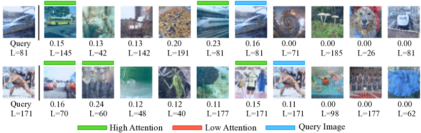
6.4 Investigating attention in ICRM
As discussed in Section 2, one special feature of ICRM is its ability to learn an amortization function by paying attention to the input query and its context. To better understand this nuanced functionality, we turn our focus to visualizing attention maps of a trained ICRM model. Specifically, we construct a random sequence of data from the test environment and examine the attention scores between each example in this sequence and a novel input query across different heads. Figure 2 illustrates attention scores from a single head for two query images (marked in blue) for FEMNIST and Tiny ImageNet-C. The top row reveal that the model selectively attends to images featuring at least two curved arcs (marked in green) while paying little attention to a partial circle (highlighted in red). Additionally, when the query image is interpreted as a 90-degree clockwise rotated digit “2”, the model extends its attention to other augmentations of “2” within the prompt. Remarkably, such attention patterns emerge on unseen domains using only unlabeled examples from them, underscoring the potential of amortization! Similarly, in the second row, attention is predominantly allocated to lines of length similar to that of the query (also in green), thereby largely disregarding shorter lines (shown in red). The last two rows in Figure 2 show that the model, when presented with a query image of a train, attends not only on other trains but also on a bus—indicating a semantic understanding of similarity. In the bottom panel, the model demonstrates a capability to discern individuals across samples within the prompt.
7 Discussion
We have introduced In-Context Risk Minimization (ICRM), a framework to address domain generalization as next-token prediction. ICRM learns in-context about environmental features by paying attention to unlabeled instances as they arrive. In such a away, ICRM dynamically zooms-in on the test environment risk minimizer, achieving competitive out-of-distribution generalization.
ICRM provides a new perspective on invariance. While prior work on DG focused on information removal as a guide to generalization, ICRM suggests that extending the feature space with the relevant environment information affords further invariance. By addressing the very general problem of next-token prediction in-distribution, we amortize the performance over many specific out-of-distribution tasks. This happens by virtue of moving beyond coarse environment indices, into rich, hierarchical, and partially-overlapping context vectors. More generally, by framing DG in terms of next-token prediciton, we enable learning machines to fully exploit data in natural order, more closely mimicking the human learning experience. As Léon Bottou once said, Nature does not shuffle data. As a word of caution, we must conduct research to guarantee that in-context learners do not “zoom-in” on toxic spurious correlations with high predictive power in certain environments.
We would like to close with a quote from Andersen et al. (2022), who claim that the central property of zooming-in on the relevant information
refers to a cognitive agent’s ability to intelligently ignore irrelevant information and zero in on those aspects of the world that are relevant to their goals. The relevance realization framework suggests that the brain achieves this feat by attempting to balance the competing goals of remaining efficient in the current environment while also being resilient in the face of environmental perturbations.
Paralleling the examples from Andersen et al. (2022), we are excited to work to further understand how next-token prediction and in-context learning serves as a powerful mechanism to amortize and dynamically navigate trade-offs such as such as the efficiency-resiliency tradeoff, the exploration-exploitation tradeoff, specialization-generalization tradeoff, and focusing-diversifying tradeoff.
Acknowledgements
We are thankful to Martin Arjovsky, Léon Bottou, Elvis Dohmatob, Badr Youbi Idrissi, Maxime Oquab, and Ahmed Touati for their valuable feedback and help.
References
- Ahuja and Lopez-Paz [2023] Kartik Ahuja and David Lopez-Paz. A closer look at in-context learning under distribution shifts. arXiv, 2023.
- Ahuja et al. [2020] Kartik Ahuja, Karthikeyan Shanmugam, Kush Varshney, and Amit Dhurandhar. Invariant risk minimization games. In ICML, 2020.
- Ahuja et al. [2021] Kartik Ahuja, Ethan Caballero, Dinghuai Zhang, Jean-Christophe Gagnon-Audet, Yoshua Bengio, Ioannis Mitliagkas, and Irina Rish. Invariance principle meets information bottleneck for out-of-distribution generalization. NeurIPS, 2021.
- Andersen et al. [2022] Brett P Andersen, Mark Miller, and John Vervaeke. Predictive processing and relevance realization: exploring convergent solutions to the frame problem. Phenomenology and the Cognitive Sciences, 2022.
- Angwin et al. [2016] Julia Angwin, Jeff Larson, Surya Mattu, and Lauren Kirchner. Machine bias. ProPublica, 2016. URL https://www.propublica.org/article/machine-bias-risk-assessments-in-criminal-sentencing.
- Arjovsky et al. [2019] Martin Arjovsky, Léon Bottou, Ishaan Gulrajani, and David Lopez-Paz. Invariant risk minimization. arXiv, 2019.
- Ash and Doléans-Dade [2000] Robert B Ash and Catherine A Doléans-Dade. Probability and measure theory. 2000.
- Bao and Karaletsos [2023] Yujia Bao and Theofanis Karaletsos. Contextual Vision Transformers for Robust Representation Learning. arXiv e-prints, 2023.
- Bengio et al. [2000] Yoshua Bengio, Réjean Ducharme, and Pascal Vincent. A neural probabilistic language model. NeurIPS, 2000.
- Blanchard et al. [2011] Gilles Blanchard, Aniket Anand Deshmukh, Ürun Dogan, Gyemin Lee, and Clayton Scott. Domain generalization by marginal transfer learning. JMLR, 2011.
- Brown et al. [2020] Tom Brown, Benjamin Mann, Nick Ryder, Melanie Subbiah, Jared D Kaplan, Prafulla Dhariwal, Arvind Neelakantan, Pranav Shyam, Girish Sastry, Amanda Askell, et al. Language models are few-shot learners. NeurIPS, 2020.
- Chang et al. [2020] Shiyu Chang, Yang Zhang, Mo Yu, and Tommi S Jaakkola. Invariant rationalization. In ICML, 2020.
- Chen et al. [2022] Yining Chen, Elan Rosenfeld, Mark Sellke, Tengyu Ma, and Andrej Risteski. Iterative feature matching: Toward provable domain generalization with logarithmic environments. NeurIPS, 2022.
- Cohen et al. [2017] Gregory Cohen, Saeed Afshar, Jonathan Tapson, and Andre Van Schaik. Emnist: Extending mnist to handwritten letters. In 2017 international joint conference on neural networks (IJCNN), 2017.
- Eastwood et al. [2022] Cian Eastwood, Alexander Robey, Shashank Singh, Julius Von Kügelgen, Hamed Hassani, George J Pappas, and Bernhard Schölkopf. Probable domain generalization via quantile risk minimization. NeurIPS, 2022.
- Finn et al. [2017] Chelsea Finn, Pieter Abbeel, and Sergey Levine. Model-agnostic meta-learning for fast adaptation of deep networks. In ICML, 2017.
- Gagnon-Audet et al. [2023] Jean-Christophe Gagnon-Audet, Kartik Ahuja, Mohammad Javad Darvishi Bayazi, Pooneh Mousavi, Guillaume Dumas, and Irina Rish. WOODS: Benchmarks for out-of-distribution generalization in time series. TMLR, 2023.
- Ganin et al. [2016] Yaroslav Ganin, Evgeniya Ustinova, Hana Ajakan, Pascal Germain, Hugo Larochelle, François Laviolette, Mario Marchand, and Victor Lempitsky. Domain-adversarial training of neural networks. JMLR, 2016.
- Gulrajani and Lopez-Paz [2020] Ishaan Gulrajani and David Lopez-Paz. In search of lost domain generalization. arXiv, 2020.
- Hendrycks and Dietterich [2019] Dan Hendrycks and Thomas Dietterich. Benchmarking neural network robustness to common corruptions and perturbations. arXiv, 2019.
- Izmailov et al. [2022] Pavel Izmailov, Polina Kirichenko, Nate Gruver, and Andrew G Wilson. On feature learning in the presence of spurious correlations. NeurIPS, 2022.
- Jin et al. [2020] Wengong Jin, Regina Barzilay, and Tommi Jaakkola. Enforcing predictive invariance across structured biomedical domains, 2020.
- Khemakhem et al. [2020] Ilyes Khemakhem, Diederik Kingma, Ricardo Monti, and Aapo Hyvarinen. Variational autoencoders and nonlinear ica: A unifying framework. In AISTATS, 2020.
- Kingma and Ba [2014] Diederik P Kingma and Jimmy Ba. Adam: A method for stochastic optimization. arXiv, 2014.
- Kirichenko et al. [2022] Polina Kirichenko, Pavel Izmailov, and Andrew Gordon Wilson. Last layer re-training is sufficient for robustness to spurious correlations. arXiv, 2022.
- Koh et al. [2021] Pang Wei Koh, Shiori Sagawa, Henrik Marklund, Sang Michael Xie, Marvin Zhang, Akshay Balsubramani, Weihua Hu, Michihiro Yasunaga, Richard Lanas Phillips, Irena Gao, et al. Wilds: A benchmark of in-the-wild distribution shifts. In ICML, 2021.
- Koyama and Yamaguchi [2020] Masanori Koyama and Shoichiro Yamaguchi. Out-of-distribution generalization with maximal invariant predictor. arXiv, 2020.
- Krueger et al. [2020] David Krueger, Ethan Caballero, Joern-Henrik Jacobsen, Amy Zhang, Jonathan Binas, Dinghuai Zhang, Remi Le Priol, and Aaron Courville. Out-of-distribution generalization via risk extrapolation (rex). arXiv, 2020.
- Lachapelle et al. [2022] Sébastien Lachapelle, Pau Rodriguez, Yash Sharma, Katie E Everett, Rémi Le Priol, Alexandre Lacoste, and Simon Lacoste-Julien. Disentanglement via mechanism sparsity regularization: A new principle for nonlinear ica. In Conference on Causal Learning and Reasoning, 2022.
- Lechner et al. [2022] Mathias Lechner, Ramin Hasani, Alexander Amini, Tsun-Hsuan Wang, Thomas A Henzinger, and Daniela Rus. Are all vision models created equal? a study of the open-loop to closed-loop causality gap. arXiv, 2022.
- Li et al. [2018] Ya Li, Mingming Gong, Xinmei Tian, Tongliang Liu, and Dacheng Tao. Domain generalization via conditional invariant representations. In Proceedings of the AAAI conference on artificial intelligence, 2018.
- Li et al. [2016] Yanghao Li, Naiyan Wang, Jianping Shi, Jiaying Liu, and Xiaodi Hou. Revisiting batch normalization for practical domain adaptation. arXiv, 2016.
- Mahajan et al. [2020] Divyat Mahajan, Shruti Tople, and Amit Sharma. Domain generalization using causal matching. arXiv, 2020.
- Makar et al. [2022] Maggie Makar, Ben Packer, Dan Moldovan, Davis Blalock, Yoni Halpern, and Alexander D’Amour. Causally motivated shortcut removal using auxiliary labels. In AISTATS, 2022.
- Menzies and Beebee [2020] Peter Menzies and Helen Beebee. Counterfactual Theories of Causation. In The Stanford Encyclopedia of Philosophy. 2020.
- Muandet et al. [2013] Krikamol Muandet, David Balduzzi, and Bernhard Schölkopf. Domain generalization via invariant feature representation. In ICML, 2013.
- Müller et al. [2020] Jens Müller, Robert Schmier, Lynton Ardizzone, Carsten Rother, and Ullrich Köthe. Learning robust models using the principle of independent causal mechanisms. arXiv, 2020.
- OpenAI [2023] OpenAI. GPT-4 Technical Report. arXiv e-prints, 2023.
- Parascandolo et al. [2021] Giambattista Parascandolo, Alexander Neitz, Antonio Orvieto, Luigi Gresele, and Bernhard Schölkopf. Learning explanations that are hard to vary. In ICLR, 2021.
- Peters et al. [2016] Jonas Peters, Peter Bühlmann, and Nicolai Meinshausen. Causal inference by using invariant prediction: identification and confidence intervals. Journal of the Royal Statistical Society Series B: Statistical Methodology, 2016.
- Radford et al. [2019] Alec Radford, Jeffrey Wu, Rewon Child, David Luan, Dario Amodei, Ilya Sutskever, et al. Language models are unsupervised multitask learners. OpenAI blog, 2019.
- Rame et al. [2022] Alexandre Rame, Corentin Dancette, and Matthieu Cord. Fishr: Invariant gradient variances for out-of-distribution generalization. In ICML, 2022.
- Robey et al. [2021] Alexander Robey, George J Pappas, and Hamed Hassani. Model-based domain generalization. arXiv, 2021.
- Rojas-Carulla et al. [2018] Mateo Rojas-Carulla, Bernhard Schölkopf, Richard Turner, and Jonas Peters. Invariant models for causal transfer learning. JMLR, 2018.
- Sagawa et al. [2019] Shiori Sagawa, Pang Wei Koh, Tatsunori B Hashimoto, and Percy Liang. Distributionally robust neural networks for group shifts: On the importance of regularization for worst-case generalization. arXiv preprint arXiv:1911.08731, 2019.
- Schmidhuber [1987] Jürgen Schmidhuber. Evolutionary principles in self-referential learning, or on learning how to learn: the meta-meta-… hook. PhD thesis, Technische Universität München, 1987.
- Shen et al. [2021] Zheyan Shen, Jiashuo Liu, Yue He, Xingxuan Zhang, Renzhe Xu, Han Yu, and Peng Cui. Towards out-of-distribution generalization: A survey. arXiv, 2021.
- Sun and Saenko [2016] Baochen Sun and Kate Saenko. Deep coral: Correlation alignment for deep domain adaptation. In Computer Vision–ECCV 2016 Workshops: Amsterdam, The Netherlands, October 8-10 and 15-16, 2016, Proceedings, Part III 14, 2016.
- Teney et al. [2020] Damien Teney, Ehsan Abbasnejad, and Anton van den Hengel. Unshuffling data for improved generalization. arXiv, 2020.
- Vapnik [1998] Vladimir Vapnik. Statistical learning theory. Wile, 1998.
- Vaswani et al. [2017] Ashish Vaswani, Noam Shazeer, Niki Parmar, Jakob Uszkoreit, Llion Jones, Aidan N Gomez, Łukasz Kaiser, and Illia Polosukhin. Attention is all you need. NeurIPS, 2017.
- Veitch et al. [2021] Victor Veitch, Alexander D’Amour, Steve Yadlowsky, and Jacob Eisenstein. Counterfactual invariance to spurious correlations in text classification. NeurIPS, 2021.
- Wald et al. [2021] Yoav Wald, Amir Feder, Daniel Greenfeld, and Uri Shalit. On calibration and out-of-domain generalization. Advances in neural information processing systems, 2021.
- Wald et al. [2023] Yoav Wald, Claudia Shi, Aahlad Puli, Amir Feder, Limor Gultchin, Mark Goldstein, Maggie Makar, Victor Veitch, and Uri Shalit. Workshop on spurious correlations, invariance and stability. ICML, 2023. URL https://icml.cc/virtual/2023/workshop/21493.
- Wang et al. [2020] Dequan Wang, Evan Shelhamer, Shaoteng Liu, Bruno Olshausen, and Trevor Darrell. Tent: Fully test-time adaptation by entropy minimization. arXiv, 2020.
- Wang et al. [2022] Haoxiang Wang, Haozhe Si, Bo Li, and Han Zhao. Provable domain generalization via invariant-feature subspace recovery. In ICML, 2022.
- Xie et al. [2023] Sang Michael Xie, Hieu Pham, Xuanyi Dong, Nan Du, Hanxiao Liu, Yifeng Lu, Percy Liang, Quoc V Le, Tengyu Ma, and Adams Wei Yu. Doremi: Optimizing data mixtures speeds up language model pretraining. arXiv preprint arXiv:2305.10429, 2023.
- Yakowitz and Spragins [1968] Sidney J Yakowitz and John D Spragins. On the identifiability of finite mixtures. The Annals of Mathematical Statistics, 1968.
- Yao et al. [2022] Huaxiu Yao, Caroline Choi, Bochuan Cao, Yoonho Lee, Pang Wei W Koh, and Chelsea Finn. Wild-time: A benchmark of in-the-wild distribution shift over time. NeurIPS, 2022.
- Zhang et al. [2020] Marvin Zhang, Henrik Marklund, Nikita Dhawan, Abhishek Gupta, Sergey Levine, and Chelsea Finn. Adaptive risk minimization: Learning to adapt to domain shift. NeurIPS, 2020.
- Zhang et al. [2023] Yihua Zhang, Pranay Sharma, Parikshit Ram, Mingyi Hong, Kush Varshney, and Sijia Liu. What is missing in irm training and evaluation? challenges and solutions. arXiv, 2023.
[appendices] \printcontents[appendices]1
Appendix
Appendix A Theorems and Proofs
A.1 Proof of Proposition 1
Lemma 1.
ICRM is Bayes optimal at all context lengths. Suppose is the cross-entropy loss and the labels are binary. The optimal in-context learner (equation 5) satisfies the following condition, i.e., for each
| (8) |
for almost all in the support of training distribution except over a set of a measure zero, and where the expectation is over conditional on . In other words, the in-context learner is Bayes optimal at each context length.
Proof.
In this result, we consider the problem of binary classification. Suppose is the probability of class . Define describing the probability of both the classes.
From equation 5, recall that the objective of ICRM is to minimize
| (9) |
Consider one of the terms in the sum above - . Substituting as the cross-entropy in this term, we obtain
If , then the second term in the above is zero and equals . Since KL divergence is always non-negative, corresponds to the lowest value that can be achieved by . If for all , then each of the terms in the sum in equation 9 are minimized. As a result, for all is a solution to equation 5.
Consider another minimizer of equation 5 and define the corresponding distribution . For each , the second term has to be zero for to be a minimizer.
If , then we claim that for almost all in the support of training distribution except over a set of measure zero. If the probability measure associated with is absolutely continuous w.r.t Lebesgue measure, then this follows from Theorem 1.6.6 [Ash and Doléans-Dade, 2000]. If the probability measure associated with is absolutely continuous w.r.t counting measure, then this trivially follows. ∎
We proved the above result for classification and cross-entropy loss for measures over that are either absolutely continuous w.r.t Lebesgue measure or the counting measure. It is easy to extend the above result for regressions and least square loss; see Lemma 1 in Ahuja and Lopez-Paz [2023].
See 1
Proof.
From Lemma 1, it follows that . The solution to empirical risk minimization , where the expectation is computed over the training distribution of conditional on . When the context is empty, then we have for almost all in the support of training distribution except over a set of measure zero. ∎
A.2 Proof of Theorem 1
See 1
Proof.
In this proof, we assume that all the concerned random variables , where is the current query and is its label and is the context preceeding it, and are discrete-valued for ease of exposition. Subsequently, we provide a proof for more general settings.
Since each is sampled independently given a training environment , we can conclude . Therefore,
Observe that for all
| (10) |
where is the set of all positive integers. The first inequality in the above follows from the fact that conditioning reduces entropy. For the second inequality, we use the following property. Consider as two random variables and define . Observe that .
Since the inequality above equation 10 holds for all , we obtain
| (11) |
Next, we argue that , which combined with equation 11 yields what we intend to prove, i.e., .
For each and in the support, we argue that . Suppose this was not true. This implies that the probability that . Since , occurs with a finite probability (as and are discrete-valued and is in the support) say , then fraction of sequences of do not converge to , which contradicts the assumption that .
Consider a from the support of , where is the current query and is the environment from which and context preceeding it is sampled. Let us consider the distribution
| (12) |
We simplify below.
| (13) |
We simplify the numerator and the denominator of the above separately below.
| (14) |
In the simplification above, we use the fact . Since converges to almost surely, the distribution takes a value one if and zero otherwise. As a result, the above expression becomes.
| (15) |
where is the set of all the environments observed conditional on with . Observe that all the environments in have the same given by . We can write
| (16) |
We simplify in a similar manner to obtain
| (17) |
| (18) |
Therefore,
| (19) |
where is any environment in , i.e., it is in the support of data sampled with and that also satisfies .
| (20) |
From equation 19, it follows that , where is any environment in . We use this in the above to get
| (21) |
∎
Proof.
We now extend the previous result to setting beyond discrete random variables. In particular, we consider settings where can be either discrete or continuous random variables. In the notation to follow, we use to denote the Radon-Nikodym derivatives. For discrete random variable, the Radon-Nikodym derivatives correspond to the standard probability mass function and for continuous random variables it would correspond to standard probability density functions. While much of the proof that follows is same as the previous proof, we repeat the arguments for completeness.
Since each is sampled independently given a training environment , we can conclude . Therefore,
Observe that for all
| (22) |
where is the set of all positive integers. The first inequality in the above follows from the fact that conditioning reduces entropy. For the second inequality, we use the following property. Consider as two random variables and define . Observe that .
Since the inequality above equation 22 holds for all , we obtain
| (23) |
Next, we argue that , which combined with equation 23 yields what we intend to prove, i.e., .
For each and in the support except over a set of probability measure zero, we argue that . Suppose this was not true. Define to be the set of values of for which . Let and the probability that . If this is true then contradicts the fact that . Therefore, .
Consider a from the support of except from , where is the current query and is the environment from which and context preceeding it is sampled. Let us consider the distribution
| (24) |
We simplify below.
| (25) |
We simplify the numerator and the denominator of the above separately.
| (26) |
In the above, we use Monotone convergence theorem to swap limit and the integrals. Since converges to almost surely, the distribution evaluates to probability one when and is zero otherwise. As a result, the above expressions become
| (27) |
where is the set of all the environments observed conditional on with . Observe that all the environments in have the same given by . Similarly,
| (28) |
As a result, we can write
We use this to obtain
| (29) |
Therefore,
| (30) |
where is any environment that is in the support of data sampled with and that also satisfies .
| (31) |
From equation 30, it follows that , where is any environment in . We use this in the above to get
| (32) |
∎
A.3 Proof of Theorem 2
See 2
Proof.
Let us consider the setting where the context is of length one. We denote the current query as with corresponding label and environment . The example in the context is which has corresponding label and it shares the same environment . Recall that as part of the context, the learner only sees and not . Both and are real-valued scalars and is a dimensional vector.
Following the assumption in the theorem, the distribution of is Markov with respect to a Bayesian network. We first establish that cannot be a child of any variable in the directed acyclic graph (DAG). The assumption implies and . Suppose is a child variable of . Due to the symmetry, and follow the same distribution. As a result, is also a child variable of , which implies (since is a collider on the path from to ). This contradicts . Suppose is a child variable of some component of say . Due to symmetry, is also a child variable of , which implies . This contradicts . Therefore, cannot be a child of any of the variables in the DAG.
Since both and form the Markov blanket of , there are two possible cases. Either is directly connected to or is connected to through some element of .
In the first case, can only have an arrow into and not the other way around as is not a child of any other node. Let us consider the setting when is one of the parents of and denote it as . Since () is on the Markov Blanket of (), we claim that each component of is either a parent of or a child of . Suppose this was not the case. This implies that there exists a component of say , which is on the Markov Blanket as a parent of . But that would make a child of . However, cannot be a child variable as shown above. As a result, each component of is either a parent or a child of . We now consider two subcases.
Let us consider the setting when there exists a child of . Observe that is a child of and it has a path to and as a result it has a path to . This path from elements of to passes through . This path has no colliders and does not contain any element of on it (We show this case in Figure 3(a)). As a result, . Thus (use chain rule of mutual information).
Let us consider the other setting when each is a parent of (shown in Figure 3(b)). In this case, has to have a path to some element of , say as otherwise , which contradicts the assumption that . Consider the path to to . Observe that this path is not blocked. As a result, .
Let us consider the other possibility when is connected to through . Here the only way this is possible is if some element of say is a child of and is a parent of that element (as shown in Figure 3(c)). Therefore, we know that is connected to through and .
Observe that this path from to is not blocked as is a collider. Therefore, . We showed the result so far assuming that the context length was one. Suppose that the context has examples denoted as . The chain rule of mutual information tells us . The proof above already demonstrates that the first term is strictly positive. Since mutual information is non-negative, we can conclude that .
Next, we want to argue that entropy strictly reduces as context length increases. In other words,
We want to show . In the proof above, we had three cases shown in Figure 3. In each of these cases, we argued that the path from to is not blocked. Even if we condition on contexts this continues to be the case. In the first two cases, the path from to is direct and does not contain any element from the conditioning set. In the third case, the direct path involves a collider from the conditioning set and thus is also not blocked. As a result, . This completes the proof.
∎
Remark on the Theorem 2
It is possible to extend Theorem 2 to the case when only a subset of and form the Markov blanket. Observe that the analysis of Case a) and Case c) in Figure 3(a), Figure 3(c) does not change. The analysis of Case b) is more nuanced now. In Case b), we used the fact that is connected to that is on the Markov blanket. This need not be the case if only a subset of is on the Markov blanket. Suppose denote the set of that are on the Markov Blanket. If is connected to any member of , the same analysis as Case b) continues to hold. Consider the case when is connected to some other member of that is not in . Denote this member as . Observe that the same element from will have a direct path into through that is not blocked. As a result, even in this case conditioning on helps.
A.4 Proof of Theorem 3
See 3
Proof.
The learning algorithm works as follows. For each pair in the training data, define the set of as . Maximize the likelihood of assuming that the underlying distribution is Gaussian. This can be stated as
The solution to the above are standard sample mean based estimators of means and covariance. Also, use a sample mean based estimator to estimate the probability of each class in environment and denote it as . Define . The model at test time works as follows.
-
•
We are given samples at test time from some environment . Estimate the parameters of Gaussian mixture model with two mixture components to maximize the likelihood of observing . We denote the estimated parameters as . Define a permutation of as .
-
•
Find the closest environment to the estimated parameters in the training set.
(33) Suppose is the closest training environment that solves the above. If is closer to than , then correspond to the label and correspond to the label . For the query , the probability assigned to label is
If is closest to this environment, then correspond to the label and is the label . For the query , the probability assigned to label is .
For the training environments, in the limit of infinitely long contexts the estimated parameters take exact values, i.e., , for all .
For the test environment, the true set of parameters that generate the data are , where . Define the permutation of as .
There can be two types of test environments. One in which the mean and covariance for both classes are identical. The method above assigns a probability of to both the classes, which is the Bayes optimal prediction. Let us consider the latter environments, where the class conditional parameters for are not the same. In the limit of infinitely long contexts at test time, there are two possible values can take, either or . This follows from identifiability of Gaussian mixtures, Yakowitz and Spragins [1968].
Consider the first case, . In this case, the equation 33 becomes
Suppose some environment solves the above optimization. Following the assumption in we know that falls in the Voronoi region of some and thus is closer to than . As a result, is associated with class , which is actually correct and thus the final predictor would match the Bayes optimal predictor for the test environment. In the second case, . Therefore, and would be correctly associated with class one thus leading to Bayes optimal predictions. This completes the argument we set out to prove.
We now briefly explain how the method fails if test parameter is outside the Voronoi cell of training parameters. Suppose but is in Voronoi region of some . In this case, would be closest to and would be incorrectly associated with class . This shows that beyond the Voronoi region the proposed algorithm fails.
∎
A.5 Extension of Theorem 3
In the previous theorem, we assumed that is identity. We now describe how the result can be extended to general non-linear mixing maps . For this result, we leverage the theoretical results from identifiable variational autoencoders (i-VAE) [Khemakhem et al., 2020].
A short review of identifiable variational autoencoders
We are provided with observations ’s that are generated from a latent variable using an injective map , where . The theory of i-VAE provides with a method and the conditions under which the underlying true latent variables can be identified up to permutation and scaling. In i-VAEs, it is assumed that along with each sample , we are provided with auxiliary information, which they term as . For our results, auxiliary information is available to us in the form of the environment index and the label of the data point. In the theory of i-VAE, the distribution of the latent variables are assumed to follow a conditionally factorial exponential distribution stated as follows.
| (34) |
where are the sufficient statistics, are the parameters of the distribution that vary with , is a base measure and is a normalizing constant. We concatenate ’s and across latent dimensions to make construct dimensional vectors denoted as and . Thus the data generation process is summarized as
| (35) |
where are the parameters. We now revisit the data generation process that we consider and explain how it falls under the umbrella of the data generation processes considered in i-VAE. For all ,
| (36) |
where the latent variables are sampled conditional on the label and environment from a Normal distribution whose mean and covariance depend on both . We further assume that the covariance matrix has a diagonal structure as stated below.
Assumption 1.
Each is a diagonal matrix.
Since is a diagonal matrix, we denote the diagonal element as . Similarly, the component of is denoted as . Observe that the distribution of conditional on belongs to the family conditionally factorial exponential distributions studied in i-VAE. If we substitute , , , , and , then we obtain the distribution of described by equation 36.
Definition 1.
We define an equivalence relation between sets of parameters of the model as follows.
| (37) |
If is invertible, then we denote the relation by . If is a block permutation matrix, then we denote it by .
Theorem 4.
Assume that the data is sampled from the data generation in equation equation 35 according to with parameters . Assume the following holds
-
•
The mixing function is injective
-
•
The sufficient statistics are differentiable almost everywhere, and are linearly independent on any subset of of measure greater than zero.
-
•
There exists distinct points such that the matrix
of size is invertible.
then the parameters are identifiable.
Theorem 5.
Assume the hypotheses of the Theorem 4 holds, and . Further assume:
-
•
The sufficient statistics are twice differentiable.
-
•
The mixing function has all second order cross derivatives.
then the parameters are identifiable.
We can leverage the above two theorems (Theorem 4, Theorem 5 and Theorem 4 from Lachapelle et al. [2022]) and arrive at the following corollary for the Gaussian data generation process from equation 36.
Theorem 6.
If the data generation process follows equation 36, where is injective and has all second order cross derivatives. Suppose there exist points in the support of observed in training distribution such that
is invertible. If for all in the support of in the training distribution, then , where and .
Proof.
We equate the probability of observations under two models and for each . Consider a and the corresponding . These ’s follow since . Define and these follow . We can write , where .
Observe
| (38) |
Substituting the exponential form we obtain that
If we use sufficient variability conditions, we obtain . We now use the fact that sufficient statistics are minimal to conclude that
where is invertible. In the above, we use the line of reasoning used in in the proof of Theorem 4 in [Lachapelle et al., 2022].
After this point, we leverage Theorem 5 to conclude that
We can expand the above to write
Note that the above relationship holds for all . If depends on , then would be a degree four polynomial in and it would be equated to a degree polynomial stated in the RHS. This cannot be true for all in the support. As a result, is a scalar multiple of . Since for every there is such a , it follows that .
∎
Theorem 7.
(Zoom-in [ood]) Consider the data generation process in equation 36. We make a few additional assumptions on the data generation stated below.
-
•
Each is a diagonal matrix
-
•
There exist points in the support of observed in training distribution such that
is invertible.
-
•
is injective and has all second order cross derivatives.
Under the above assumptions, we can guarantee that there exists an in-context learning algorithm that generates Bayes optimal predictions for all the test environments that fall in Voronoi cells of training parameters weighted by a certain vector.
Proof.
The training proceeds as follows. Train an autoencoder on training data under the constraint that the output of the encoder follow a Gaussian distribution with independent components conditional on each . This is stated as the following minimization.
| (39) |
where , is the distribution of . The first term is standard reconstruction loss and the second term is the KL divergence between distribution of and a Normal distribution with independent components. Also, estimate the class probabilities for each environment and denote them as . Similar to the proof of Theorem 3 define
The model at test time works as follows. We first use the trained encoder and generate for test time inputs. After this the model operates in exactly the same way on as in the proof of Theorem 3. Basically the output of encoder takes place of raw ’s in the procedure described in proof of Theorem 3.
The assumptions in this theorem along with following i) follows a Gaussian distribution with independent components, ii) follows distribution of conditional on for each , implies we can use the previous result in Theorem 6 to conclude that . Observe that also follows a Gaussian distribution with independent components conditional on each . In the limit of infinitely long contexts, is equal to scaled means of original training environments and covariances also scaled componentwise according to the transform . We can now apply the previous Theorem 3 on as follows. If the parameters of the test environment are in the Voronoi cell of the train distribution of , then the procedure described above continues to generate Bayes optimal predictions in those environments.
∎
A.6 Comparing ICRM and ERM under the lens of invariance
The label is related to and mean of in environment as follows.
| (40) |
ERM learns a linear model on features . The closed form solution for linear regression is , where , which is assumed to be invertible, and . The covariance matrix of is defined as
Proposition 2.
Let for all . If is invertible, , , for some , then the coefficient estimated by ERM for is not the same as the invariant coefficient .
Proof.
We compute first.
| (41) |
where
Next, we compute .
| (42) |
The solution to ERM is
| (43) |
Simplifying the above, we obtain the coefficient for to be
| (44) |
Owing to the assumptions, and for some we obtain that the second term in the above is not zero. As a result, the estimate computed by ERM for is biased. ∎
Proposition 3.
Let for all . If is invertible, , , . The error of ERM in test environment increases in
Proof.
The error of ERM is given as
| (45) |
where is the variance of the noise variable . If we take the derivative of the above error w.r.t , we obtain , which is positive. This completes the proof.
∎
ICRM learns a linear model on . We study two settings to analyze the error of ICRM at test time. If at test time, the model has seen sufficiently long contexts, then it knows the means corresponding to and and the model achieves the test error of . On the other hand, if the context is empty, then also note that the expected error of the model is (assuming the model uses a default value of zero for the mean in the absence of any context), where is the mean of in environment . Since the error of ICRM in the absence of any context is independent of variance of , the error of ERM can be much worse than that of ICRM in this setting as well.
Moving forward let us consider a more general setting.
| (46) |
where and are maps (potentially non-linear), and are independent zero mean noise variables. Following the same line of thought as the above example. ICRM learns a non-linear model on and learns . From equation 46, it follows that
From the above it follows that ICRM learns . In comparison, consider standard ERM learns a non-linear model on . Consider the DAG corresponding to setting equation 46. We assume that the joint distribution described in equation 46 is Markov w.r.t to the following DAG . As a result, . This follows from the fact there is a path to through and is not blocked by . From it follows that ERM learns a predictor that relies on both and . Therefore, ICRM learns the right invariant model and does not rely on and ERM relies on spurious feature .
A.7 Illustration of failure of existing MTL methods
In this section, we provide a simple example to show the failure mode of marginal transfer learning (MTL) methods that are based on averaging to summarize information about the environment. These methods can be summarized to take the following form:
| (47) |
We are only going to consider maps that are differentiable.
Example.
Suppose we want to learn the following function
| (48) |
where is the input in the context and is the current query. We claim that if for all , then the output dimension of grows in context length . Suppose this was not the case. If output dimension is smaller than , then cannot be a differentiable bijection. As a result, there exists two contexts and of same length for which . We argue that there exists an such that . This would lead to a contradiction as for all . Without loss of generality, suppose that the smallest value of context is smaller than that in context . If is larger than smallest value of but lesser than smallest value of , then on the other hand .
Appendix B Related work
A brief tour of domain generalization.
Muandet et al. [2013] developed kernel methods to learn transformations such that the distance between the feature distributions across domains is minimized and the information between the features and the target labels is preserved. The pioneering work of Ganin et al. [2016] proposes a method inspired from generative adversarial networks to learn feature representations that are similar across domains. Sun and Saenko [2016] developed a method based on a natural strategy to match the means and covariances of feature representations across domains. Li et al. [2018] went a step further to enforce invariance on the distribution of representations conditional on the labels. In a parallel line of work, led by Peters et al. [2016], Rojas-Carulla et al. [2018], Arjovsky et al. [2019], the proposals sought to learn representations such that the distribution of labels conditional on the representation are invariant across domains. These works were followed by several interesting proposals to enforce invariance – [Teney et al., 2020, Krueger et al., 2020, Ahuja et al., 2020, Jin et al., 2020, Chang et al., 2020, Mahajan et al., 2020, Koyama and Yamaguchi, 2020, Müller et al., 2020, Parascandolo et al., 2021, Ahuja et al., 2021, Robey et al., 2021, Wald et al., 2021, Chen et al., 2022, Wang et al., 2022, Zhang et al., 2023, Eastwood et al., 2022, Rame et al., 2022, Veitch et al., 2021, Makar et al., 2022] – which is an incomplete representative list. See Shen et al. [2021] for a more comprehensive survey of these works. Most of the above works have focused on learning features that enable better generalization. Recently there been an intriguing line of work from Kirichenko et al. [2022], Izmailov et al. [2022] that shifts the focus from feature learning to last layer retraining. These works show that under certain conditions (e.g., avaiability of some data that does not carry spurious correlations) one can carry out last layer retraining and achieve significant out-of-distribution performance improvements.
In the main body of the paper, we already discussed the other prominent line of work in domain generalization on marginal transfer learning, where the focus is to leverage the distributional features and learn environment specific relationships. This line of work was started by the notable work of Blanchard et al. [2011] and has been followed up by several important proposals such as Zhang et al. [2020], Bao and Karaletsos [2023].
Appendix C Supplementary experimental details and assets disclosure
C.1 Assets
We do not introduce new data in the course of this work. Instead, we use publicly available widely used image datasets for the purposes of benchmarking and comparison.
C.2 Hardware and setup
Each experiment was performed on 8 NVIDIA Tesla V100 GPUs with 32GB accelerator RAM for a single training run. The CPUs used were Intel Xeon E5-2698 v4 processors with 20 cores and 384GB RAM. All experiments use the PyTorch deep-learning framework
C.3 Datasets
C.3.1 Federated Extended MNIST (FEMNIST)
Building on the Extended MNIST (EMNIST) dataset, which includes images of handwritten uppercase and lowercase alphabets along with digits, FEMNIST enriches this data by attributing each data point to its originating writer. This extension associates each 2828-sized image in the dataset to one of the 62 classes. In our setup, each writer serves as a distinct environment. We evaluate the performance of each method based on both worst-case and average accuracy across a set of 35 test users, who are distinct from the 262 training users and 50 validation users. Unlabelled data from an environment in this dataset could provide cues about the writing style of the user and disambiguate data points.
C.3.2 Rotated MNIST
We employ a customized version of the MNIST dataset as in Zhang et al. [2020]. The dataset contains images rotated in increments of 10 degrees, ranging from 0 to 130 degrees. Each degree of rotation constitutes a separate environment, effectively acting as a distinct value. The training set for the two most extreme rotations, 120 and 130 degrees, contains only 108 data points each. For rotations between 90 and 110 degrees, each environment includes 324 data points. The total training set comprises 32,292 points. For evaluation, test images are generated from the MNIST test set, and are duplicated for each environment. Performance metrics include both worst-case and average accuracy across these testing domains. Analogous to FEMNIST, unlabeled samples from an environment within this dataset can assist in distinguishing images that may seem similar due to their rotated orientations.
C.3.3 WILDS Camelyon17
We use the Camelyon17 dataset, part of the WILDS benchmark [Koh et al., 2021], which features image patches derived from whole-slide lymph node sections of patients with potential metastatic breast cancer. Each patch is labeled to indicate the presence or absence of a tumor. In our experimental design, each participating hospital is treated as a distinct environment. The dataset is partitioned in alignment with the official WILDS configuration: three hospitals contribute to the training set, a fourth is designated for validation, and the remaining hospital’s data is used for testing.
C.3.4 Tiny ImageNet-C
Adapting the methodology from Hendrycks and Dietterich [2019], we introduce 56 distinct distortions to the training set, treating each as a separate environment. For evaluation, we use a non-overlapping set of 22 test distortions, largely differing in nature from those used in training. Each 64X64-sized distorted image is associated with one of the 200 classes in the dataset. This setup permits an investigation into whether exposure to distortions during training equips the model to better manage novel distortions during testing. We assess performance through both worst-case and average accuracies across these test distortions.
C.4 Experimental protocols
To ensure a fair comparison across different algorithms for each dataset, we use a standardized neural network backbone. The details for these architectures are provided in Section C.4 and Section C.4. We use the ConvNet architecture as outlined in Zhang et al. [2020].
For ICRM, the same backbone is used to featurize the input, which is then processed by the decoder-only Transformer [Vaswani et al., 2017] architecture from the GPT-2 Transformer family [Radford et al., 2019]. Our model is standardized to have 12 layers, 4 attention heads, and a 128-dimensional embedding space across all datasets. Linear layers are employed to map both the input sequence to the transformer’s latent embedding and the model’s predicted output vector to the output label. For training ICRM on larger datasets like WILDS Camelyon17 and Tiny ImageNet-C, we start with a ResNet50 model pre-trained on ImageNet (as shown in Section C.4) and freeze all batch normalization layers before fine-tuning.
We adopt the same Context Network as used in ARM, specifically retaining their choice of output channels – one for smaller datasets like FEMNIST and Rotated MNIST, and three for the others.
For TENT, all reported metrics are based on its episodic version, where the model is reset to its trained state after processing each batch. This ensures a fair comparison with other methods. Additionally, during testing, the model’s parameters are updated for 10 steps using stochastic gradient descent by minimization test entropy across all datasets.
| Dataset | Architecture | |
|---|---|---|
| ICRM | Others | |
| FEMNIST | ConvNet + GPT2 Transformer | ConvNet |
| Rotated MNIST | ||
| Camelyon17 | ResNet-50 + GPT2 Transformer | ResNet-50 |
| Tiny ImageNet-C | ||
| # | Layer |
|---|---|
| 1 | Conv2D (in=, out=128) |
| 2 | BatchNorm2d (dim=129) |
| 3 | ReLU |
| 4 | Max Pooling (2) |
| 5 | Conv2D (in=128, out=128) |
| 6 | BatchNorm2d (dim=128) |
| 7 | ReLU |
| 8 | Max Pooling (2) |
| 9 | Global average-pooling |
We list all hyperparameters, their default settings, and search boundaries for random sweeps in Table 7. The maximum context length, or support, is fixed at 100 for all algorithms. All models are optimized using the Adam optimizer [Kingma and Ba, 2014]. To ensure a fair comparison, we perform a random search of 5 trials across the hyperparameter range (refer to Table 7) for each algorithm. The model with the highest validation set accuracy is selected for each run. We then report the average of this number across three independent runs of the entire sweep, and its corresponding standard error.
| Condition | Parameter | Default value | Random distribution |
|---|---|---|---|
| ResNet | learning rate | 0.0001 | |
| weight decay | 0 | ||
| not ResNet | learning rate | 0.0001 | |
| weight decay | 0 |
Appendix D Additional experiments
D.1 Adaptation curves of various algorithms
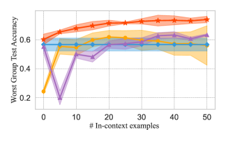
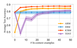
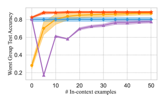
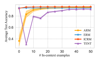
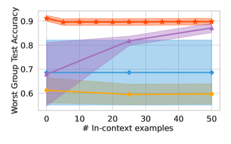
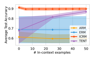
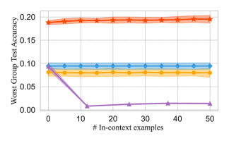
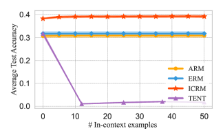
D.2 Domain generalization accuracies per algorithm and dataset
| Dataset / algorithm | Average test accuracy (by # in-context examples) | ||||
|---|---|---|---|---|---|
| FEMNIST | 0 | 25 | 50 | 75 | 100 |
| ARM | 49.5 1.0 | 83.9 0.5 | 84.4 0.5 | 84.7 0.6 | 84.6 0.3 |
| TENT | 78.1 1.2 | 77.9 1.2 | 81.2 0.9 | 82.5 0.9 | 83.3 0.8 |
| ERM | 79.3 0.4 | 79.3 0.4 | 79.3 0.4 | 79.3 0.4 | 79.3 0.4 |
| ICRM | 78.7 0.5 | 87.2 0.4 | 87.4 0.5 | 87.5 0.2 | 87.8 0.2 |
| Rotated MNIST | 0 | 25 | 50 | 75 | 100 |
| ARM | 36.5 5.2 | 94.2 0.7 | 95.1 0.4 | 95.3 0.4 | 95.5 0.3 |
| TENT | 94.1 0.3 | 88.0 0.4 | 91.9 0.3 | 93.8 0.2 | 94.3 0.2 |
| ERM | 94.2 0.3 | 94.2 0.3 | 94.2 0.3 | 94.2 0.3 | 94.2 0.3 |
| ICRM | 93.6 0.2 | 96.1 0.1 | 96.2 0.1 | 96.2 0.1 | 96.2 0.1 |
| WILDS Camelyon17 | 0 | 25 | 50 | 75 | 100 |
| ARM | 61.2 5.2 | 59.5 4.2 | 59.7 4.2 | 59.7 4.3 | 59.7 4.2 |
| TENT | 67.9 7.6 | 81.8 1.1 | 87.2 1.1 | 89.4 1.1 | 89.4 1.0 |
| ERM | 68.6 7.8 | 68.6 7.8 | 68.6 7.8 | 68.6 7.8 | 68.6 7.8 |
| ICRM | 92.0 0.6 | 90.7 0.8 | 90.8 0.8 | 90.8 0.8 | 90.8 0.8 |
| Tiny ImageNet-C | 0 | 25 | 50 | 75 | 100 |
| ARM | 30.8 0.2 | 31.0 0.2 | 31.0 0.2 | 31.0 0.2 | 31.0 0.2 |
| TENT | 31.7 0.5 | 1.6 0.1 | 1.7 0.1 | 2.0 0.1 | 2.1 0.1 |
| ERM | 31.8 0.6 | 31.8 0.6 | 31.8 0.6 | 31.8 0.6 | 31.8 0.6 |
| ICRM | 38.3 0.1 | 39.2 0.3 | 39.2 0.3 | 39.2 0.3 | 39.2 0.3 |
| Dataset / algorithm | Worst case test accuracy (by # in-context examples) | ||||
|---|---|---|---|---|---|
| FEMNIST | 0 | 25 | 50 | 75 | 100 |
| ARM | 23.6 1.7 | 59.5 3.5 | 60.7 3.8 | 57.0 7.3 | 58.8 4.0 |
| TENT | 55.2 2.5 | 57.2 2.2 | 63.3 0.4 | 65.9 0.6 | 67.2 1.0 |
| ERM | 59.0 0.2 | 59.0 0.2 | 59.0 0.2 | 59.0 0.2 | 59.0 0.2 |
| ICRM | 59.8 0.7 | 69.3 0.0 | 70.6 2.3 | 70.6 1.5 | 70.6 0.7 |
| Rotated MNIST | 0 | 25 | 50 | 75 | 100 |
| ARM | 28.2 2.1 | 85.3 1.6 | 87.2 1.0 | 87.9 1.0 | 87.9 0.9 |
| TENT | 80.2 1.3 | 88.5 0.8 | 88.5 0.9 | 80.2 1.0 | 81.3 1.0 |
| ERM | 80.8 1.1 | 80.8 1.1 | 80.8 1.1 | 80.8 1.1 | 80.8 1.1 |
| ICRM | 82.5 0.5 | 88.5 0.5 | 88.5 0.5 | 88.8 0.5 | 88.8 0.4 |
| WILDS Camelyon17 | 0 | 25 | 50 | 75 | 100 |
| ARM | 61.2 5.2 | 59.5 4.2 | 59.7 4.2 | 59.7 4.3 | 59.7 4.2 |
| TENT | 67.9 7.6 | 81.8 1.1 | 87.2 1.1 | 89.4 1.1 | 89.4 1.0 |
| ERM | 68.6 7.8 | 68.6 7.8 | 68.6 7.8 | 68.6 7.8 | 68.6 7.8 |
| ICRM | 92.0 0.6 | 90.7 0.8 | 90.8 0.8 | 90.8 0.8 | 90.8 0.8 |
| Tiny ImageNet-C | 0 | 25 | 50 | 75 | 100 |
| ARM | 8.2 0,3 | 8.3 0.3 | 8.2 0.3 | 8.3 0.3 | 8.2 0.3 |
| TENT | 1.2 0.4 | 1.4 0.0 | 1.6 0.1 | 1.6 0.0 | 1.6 0.0 |
| ERM | 9.5 0.4 | 9.5 0.4 | 9.5 0.4 | 9.5 0.4 | 9.5 0.4 |
| ICRM | 18.8 0.2 | 19.2 0.1 | 19.5 0.2 | 19.5 0.1 | 19.4 0.2 |
| Dataset / algorithm | Average test accuracy (by # in-context examples) | ||||
|---|---|---|---|---|---|
| FEMNIST | 0 | 25 | 50 | 75 | 100 |
| ICRM | 78.7 0.5 | 87.2 0.4 | 87.4 0.5 | 87.5 0.2 | 87.8 0.2 |
| ICRM-Mix | 77.6 0.8 | 81.1 0.2 | 81.1 0.2 | 80.9 0.3 | 80.9 0.1 |
| Rotated MNIST | 0 | 25 | 50 | 75 | 100 |
| ICRM | 93.6 0.2 | 96.1 0.1 | 96.2 0.1 | 96.2 0.1 | 96.2 0.1 |
| ICRM-Mix | 88.9 1.4 | 92.6 0.3 | 92.7 0.2 | 92.6 0.3 | 92.7 0.2 |
| WILDS Camelyon17 | 0 | 25 | 50 | 75 | 100 |
| ICRM | 92.0 0.6 | 90.7 0.8 | 90.8 0.8 | 90.8 0.8 | 90.8 0.8 |
| ICRM-Mix | 92.9 0.3 | 90.7 0.6 | 90.8 0.5 | 90.7 0.5 | 90.7 0.5 |
| Tiny ImageNet-C | 0 | 25 | 50 | 75 | 100 |
| ICRM | 38.3 0.1 | 39.2 0.3 | 39.2 0.3 | 39.2 0.3 | 39.2 0.3 |
| ICRM-Mix | 38.4 0.2 | 39.3 0.2 | 39.3 0.2 | 39.3 0.2 | 39.3 0.2 |
| Dataset / algorithm | Worst case test accuracy (by # in-context examples) | ||||
|---|---|---|---|---|---|
| FEMNIST | 0 | 25 | 50 | 75 | 100 |
| ICRM | 59.8 0.7 | 69.3 0.0 | 70.6 2.3 | 70.6 1.5 | 70.6 0.7 |
| ICRM-Mix | 57.5 1.4 | 62.7 1.1 | 65.0 0.3 | 64.1 1.5 | 62.9 2.3 |
| Rotated MNIST | 0 | 25 | 50 | 75 | 100 |
| ICRM | 82.5 0.5 | 88.5 0.5 | 88.5 0.5 | 88.8 0.5 | 88.8 0.4 |
| ICRM-Mix | 68.8 3.8 | 77.1 0.7 | 76.8 0.9 | 76.4 0.9 | 76.6 0.9 |
| WILDS Camelyon17 | 0 | 25 | 50 | 75 | 100 |
| ICRM | 92.0 0.6 | 90.7 0.8 | 90.8 0.8 | 90.8 0.8 | 90.8 0.8 |
| ICRM-Mix | 92.9 0.3 | 90.7 0.6 | 90.8 0.5 | 90.7 0.5 | 90.7 0.5 |
| Tiny ImageNet-C | 0 | 25 | 50 | 75 | 100 |
| ICRM | 18.8 0.2 | 19.2 0.1 | 19.5 0.2 | 19.5 0.1 | 19.4 0.2 |
| ICRM-Mix | 18.7 0.2 | 19.2 0.2 | 19.4 0.1 | 19.5 0.1 | 19.4 0.1 |
| Dataset / algorithm | Average test accuracy (by # in-context examples) | ||||
|---|---|---|---|---|---|
| FEMNIST | 0 | 25 | 50 | 75 | 100 |
| ARM | 49.5 1.0 | 83.9 0.5 | 84.4 0.5 | 84.7 0.6 | 84.6 0.3 |
| ARM+ | 71.4 1.2 | 83.4 0.2 | 84.0 0.2 | 83.8 0.2 | 83.5 0.1 |
| ERM | 79.3 0.4 | 79.3 0.4 | 79.3 0.4 | 79.3 0.4 | 79.3 0.4 |
| ERM+ | 77.4 1.3 | 77.4 1.3 | 77.4 1.3 | 77.4 1.3 | 77.4 1.3 |
| Rotated MNIST | 0 | 25 | 50 | 75 | 100 |
| ARM | 36.5 5.2 | 94.2 0.7 | 95.1 0.4 | 95.3 0.4 | 95.5 0.3 |
| ARM+ | 86.9 2.0 | 92.6 0.7 | 92.7 0.6 | 92.8 0.6 | 92.8 0.6 |
| ERM | 94.2 0.3 | 94.2 0.3 | 94.2 0.3 | 94.2 0.3 | 94.2 0.3 |
| ERM+ | 94.3 0.4 | 94.3 0.4 | 94.3 0.4 | 94.3 0.4 | 94.3 0.4 |
| WILDS Camelyon17 | 0 | 25 | 50 | 75 | 100 |
| ARM | 61.2 5.2 | 59.5 4.2 | 59.7 4.2 | 59.7 4.3 | 59.7 4.2 |
| ARM+ | 55.8 0.8 | 55.1 1.7 | 55.0 1.7 | 55.0 1.8 | 55.0 1.8 |
| ERM | 68.6 7.8 | 68.6 7.8 | 68.6 7.8 | 68.6 7.8 | 68.6 7.8 |
| ERM+ | 50.1 0.1 | 50.1 0.1 | 50.1 0.1 | 50.1 0.1 | 50.1 0.1 |
| Tiny ImageNet-C | 0 | 25 | 50 | 75 | 100 |
| ARM | 30.8 0.2 | 31.0 0.2 | 31.0 0.2 | 31.0 0.2 | 31.0 0.2 |
| ARM+ | 5.5 0.2 | 5.7 0.2 | 5.7 0.2 | 5.7 0.2 | 5.7 0.2 |
| ERM | 31.8 0.6 | 31.8 0.6 | 31.8 0.6 | 31.8 0.6 | 31.8 0.6 |
| ERM+ | 29.7 0.3 | 29.7 0.3 | 29.7 0.3 | 29.7 0.3 | 29.7 0.3 |
| Dataset / algorithm | Worst case test accuracy (by # in-context examples) | ||||
|---|---|---|---|---|---|
| FEMNIST | 0 | 25 | 50 | 75 | 100 |
| ARM | 23.6 1.7 | 59.5 3.5 | 60.7 3.8 | 57.0 7.3 | 58.8 4.0 |
| ARM+ | 51.7 2.2 | 63.0 2.1 | 64.0 0.8 | 60.7 1.6 | 62.0 0.8 |
| ERM | 59.0 0.2 | 59.0 0.2 | 59.0 0.2 | 59.0 0.2 | 59.0 0.2 |
| ERM+ | 53.3 2.7 | 53.3 2.7 | 53.3 2.7 | 53.3 2.7 | 53.3 2.7 |
| Rotated MNIST | 0 | 25 | 50 | 75 | 100 |
| ARM | 28.2 2.1 | 85.3 1.6 | 87.2 1.0 | 87.9 1.0 | 87.9 0.9 |
| ARM+ | 71.4 2.6 | 80.9 1.8 | 81.0 1.8 | 81.2 1.9 | 81.1 1.8 |
| ERM | 80.8 1.1 | 80.8 1.1 | 80.8 1.1 | 80.8 1.1 | 80.8 1.1 |
| ERM+ | 81.9 0.7 | 81.9 0.7 | 81.9 0.7 | 81.9 0.7 | 81.9 0.7 |
| WILDS Camelyon17 | 0 | 25 | 50 | 75 | 100 |
| ARM | 61.2 5.2 | 59.5 4.2 | 59.7 4.2 | 59.7 4.3 | 59.7 4.2 |
| ARM+ | 55.8 0.8 | 55.1 1.7 | 55.0 1.7 | 55.0 1.8 | 55.0 1.8 |
| ERM | 68.6 7.8 | 68.6 7.8 | 68.6 7.8 | 68.6 7.8 | 68.6 7.8 |
| ERM+ | 50.1 0.1 | 50.1 0.1 | 50.1 0.1 | 50.1 0.1 | 50.1 0.1 |
| Tiny ImageNet-C | 0 | 25 | 50 | 75 | 100 |
| ARM | 8.2 0.3 | 8.3 0.3 | 8.2 0.3 | 8.3 0.3 | 8.2 0.3 |
| ARM+ | 1.9 0.1 | 1.9 0.1 | 1.9 0.1 | 1.9 0.1 | 1.9 0.1 |
| ERM | 9.5 0.4 | 9.5 0.4 | 9.5 0.4 | 9.5 0.4 | 9.5 0.4 |
| ERM+ | 8.3 0.3 | 8.3 0.3 | 8.3 0.3 | 8.3 0.3 | 8.3 0.3 |