Probing the photon emissivity of the quark-gluon plasma
without an inverse problem in lattice QCD

Abstract

The thermal photon emissivity of the quark-gluon plasma is determined by the in-medium spectral function of the electromagnetic current at lightlike kinematics, $\sigma(\omega)$. In this work, we present the first lattice QCD results on moments of $\sigma(\omega)/\omega$, defined by the weight function $1/(\omega^{2}+(2\pi Tn)^{2})$, $n\in\mathbb{Z}$ and computed without encountering an inverse problem. We employ two dynamical flavours of O($a$)-improved Wilson fermions at a temperature $T\approx 250\;$MeV and perform the continuum limit. We compare our results for the first two moments to those obtained dispersively by integrating over the spectral function computed at weak coupling by Arnold, Moore and Yaffe.

I Introduction

The strongly-interacting matter created during a heavy-ion collision radiates electromagnetic energy due to the interactions of its charged constituents. Photons, the quanta of this radiation, have a large mean free path compared to the strongly-interacting degrees of freedom, thanks to the hierarchy of the electromagnetic and strong coupling constants at experimentally accessible temperatures, $\alpha_{\mathrm{em}}\simeq 1/137\ll\alpha_{s}$. These probes escape from the strongly interacting medium and can inform us about its entire space-time evolution.

Let $\omega$ be the energy of a photon emitted from a fluid cell at rest and in thermal equilibrium. The differential rate of photon emission per unit volume of the cell is described to all orders in the strong coupling, and to leading order in the electromagnetic coupling by the formula McLerran and Toimela (1985)

$$\frac{\mathrm{d}\Gamma_{\gamma}(\omega)}{\mathrm{d}\omega} =\frac{\alpha_{\mathrm{em}}}{\pi}\frac{2\omega\sigma(\omega)}{\mathrm{e}^{\omega/T}-1}+\mathrm{O}(\alpha_{\mathrm{em}}^{2}),$$ (1)

where $\sigma(\omega)$ is the in-medium spectral function associated with the two-point correlation function of the electromagnetic current at zero-virtuality. Therefore, this temperature-dependent spectral function directly determines the emissivity of real photons from thermal matter described by quantum chromodynamics (QCD). From the experimentally measured spectrum of photons, one would hope to infer interesting physical properties of the thermal medium, starting with its temperature. However, since the QCD matter created in a heavy-ion collision does not remain in equilibrium, the prediction of the total yield is complicated by the necessity to integrate over the spacetime history of the expanding fluid as well as to include non-thermal components David (2020).

Nevertheless, recent experimental results from the RHIC and the LHC facilities have been compared to phenomenological models which incorporate a thermal component produced by the expanding plasma Gale et al. (2021). Data for the yield of direct photons from the PHENIX and ALICE experiments at RHIC and the LHC, respectively, show an excess of production in the region of phase space where thermal sources dominate, i.e. for transverse momenta, $p_{\mathrm{T}}$, below a few $\mathrm{GeV}$ Acharya et al. (2022); Adare et al. (2015); Adam et al. (2016); Gale et al. (2021). In contrast, data from the STAR experiment at RHIC appear to be in agreement with the available theoretical models Adamczyk et al. (2017). Furthermore, the anisotropy of the photon momentum distribution, the photon $v_{2}$, is larger for all experiments than models suggest Adare et al. (2012, 2016); Acharya et al. (2019).

The failure of most models in describing collectively the experimental findings mentioned above is usually referred to as the direct photon puzzle David (2020); Geurts and Tripolt (2023); Gale et al. (2021). The model calculations rely on theoretical predictions of the thermal photon emissivity, which is directly proportional to $\sigma(\omega)$. So far, the phenomenological models have used such predictions obtained at leading order in QCD perturbation theory Arnold et al. (2001a, b), complemented with relativistic kinetic theory calculations in a hot meson gas for the hadronic phase (see e.g. Paquet et al. (2016); Turbide et al. (2004)). How exactly to connect these predictions in the vicinity of the crossover temperature of about 150 MeV is unclear, hence interpolations have been used.

Lattice QCD is a suitable framework for the non-perturbative determination of the correlation function which mathematically determines $\sigma(\omega)$ uniquely. However, given that lattice QCD is formulated in Euclidean space, obtaining the spectral density by analytic continuation from the current correlator is a numerically ill-posed problem (see for instance the reviews Meyer (2011); Aarts and Nikolaev (2021)). The analytic continuation needed to determine real-time quantities from the correlators computed in Euclidean spacetime is further hampered by the fact that a relatively small number of noisy data points are available, usually $\mathcal{O}(10-50)$ at finite temperature. Yet what one is interested in is determining a spectral function at $\mathcal{O}(1000)$ values of $\omega$ covering the interesting kinematical region with a sufficiently high resolution and with a few-percent precision.

Aiming at a goal which is within reach of the current numerical capabilities, one can try to extract not the spectral function itself, but a smeared version thereof. In the method originally proposed by G. E. Backus and J. F. Gilbert Backus and Gilbert (1968, 1970), the calculation of a smeared, filtered spectral function is viable after determining certain coefficients that multiply the Euclidean correlator data points. The value at a given $\omega$ of this smeared spectral function is a weighted average of the actual spectral function over the vicinity of $\omega$. The weighted average is defined as an integral over the spectral function multiplied by a compact kernel centered at a certain value of $\omega$. This method has been applied to several problems Brandt et al. (2016); Hansen et al. (2017); Cè et al. (2022a, b); Altenkort et al. (2022); Astrakhantsev et al. (2020, 2018); Alexandrou et al. (2023) in lattice QCD, and similar approaches have been proposed which offer a path to reducing the width of the filtering kernel, thus getting closer to the unsmeared spectral function Hansen et al. (2019); Bulava et al. (2022); Gambino et al. (2022). These approaches have in common that they provide information about an integral over the spectral function based on the Euclidean correlator and additional technical ingredients.

In this work, we obtain integrals over $\sigma(\omega)$ by calculating a correlator directly accessible in lattice QCD that has be shown Meyer (2018) to have a simple integral representation in terms of $\sigma(\omega)$. The key ingredients are to write a dispersion relation for the Euclidean correlator at fixed photon virtuality, rather than at fixed spatial momentum, and to employ an imaginary spatial momentum in order to realize lightlike kinematics in Euclidean space. We thus obtain information about the spectral function at lightlike kinematics without facing an inverse problem. This cannot be achieved when employing dispersion relations at fixed spatial photon momentum, which has been the only type of dispersion relation applied to date in lattice-QCD based studies of non-equilibrium properties of the quark-gluon plasma, starting with Ref. Karsch and Wyld (1987).

Specifically, we compute the first two moments of $\sigma(\omega)/\omega$, defined by the weight function $1/(\omega^{2}+(2\pi Tn)^{2})$ for $n=1$ and $n=2$. The construction makes use of the spatially transverse Euclidean correlator evaluated at Matsubara frequency $\omega_{n}$ and at imaginary spatial momentum, $k=\mathrm{i}\omega_{n}$. Such an ‘imaginary momentum’ corresponds to a weight function $\exp(\omega_{n}x_{3})$ in the spatial coordinate $x_{3}$, which strongly enhances the contribution from large positive $x_{3}$. Thus the control over the statistical fluctuations at long distances is the main difficulty in computing these observables in lattice QCD. Numerically, the task thus bears a strong resemblance with the lattice calculation of the hadronic vacuum polarization contribution to the muon $g-2$ Meyer and Wittig (2019); Aoyama et al. (2020); Borsanyi et al. (2021). Using the spectral function $\sigma(\omega)$ computed in QCD at weak coupling Arnold et al. (2001a, b), as well as that computed in strongly coupled super-Yang-Mills by AdS/CFT methods Caron-Huot et al. (2006a), we compute the same moments and compare them to our results. It is the first time that the weak-coupling QCD predictions for the photon emissivity of the quark-gluon plasma can be tested non-perturbatively without any uncertainties associated with an ill-posed inverse problem.

The structure of the paper is the following: In Sec. II.1, we introduce the basic observables in the continuum. In Sec. II.2, we discuss various subtractions that are necessary to reduce large cutoff effects afflicting our primary observable, while Sec. II.3 discusses the virtuality dependence of this observable. The lattice observables are defined in Sec. II.4. Thereafter, in Sec. II.5, we provide some details about our numerical setup. This is followed by the presentation of the main results in Sec. III and Sec. IV, in which we devote different subsections to the different derived observables that we investigated and describe our analysis for the sectors $n=1$ and $n=2$, respectively. In Sec. V, we compare our results to predictions made using either free quarks, the weak-coupling expansion or the strongly-coupled $\mathcal{N}=4$ super Yang-Mills theory (SYM). Finally, we conclude in Sec. VI.

II Preliminaries

II.1 Definitions in the continuum

The spectral function of the electromagnetic current is defined as

$$\rho_{\mu\nu}(\omega,{\bf k})=\int\mathrm{d}^{4}x\,e^{\mathrm{i}(\omega t-{\bf k}{\bf x})}\,\langle[J_{\mu}^{\rm{em}}(x),J_{\nu}^{\rm{em}}(0)^{\dagger}]\rangle.$$ (2)

Here, $J_{\mu}^{\rm{em}}(x)=\sum_{f}Q_{f}\bar{\psi}_{f}(x)\gamma_{\mu}\psi_{f}(x)$ is the electromagnetic current, $Q_{f}\in\{2/3,-1/3\}$ denotes the charge of a quark with flavor $f$ and $\gamma_{\mu}$ are the Euclidean Dirac matrices satisfying $\{\gamma_{\mu},\gamma_{\nu}\}=2\delta_{\mu\nu}$, i.e. ${\gamma_{\mu}}^{\dagger}=\gamma_{\mu}$. The time evolution is given in real time by $J_{\mu}^{\rm{em}}(x)=e^{\mathrm{i}Ht}J_{\mu}^{\rm{em}}(0)e^{-\mathrm{i}Ht}$. The expectation value is taken with respect to the thermal density matrix $\mathrm{e}^{-\beta H}/Z$, where $Z$ is the grand canonical partition function, $H$ is the QCD Hamiltonian and $\beta=1/T$ is the inverse temperature. The thermal photon production rate per unit volume of the QGP, $\mathrm{d}\Gamma_{\gamma}(\omega)/{\mathrm{d}\omega}$, is related to the transverse channel spectral function evaluated at lightlike kinematics, $\sigma(\omega)\equiv\rho_{\mathrm{T}}(\omega,k=\omega)$, where

$$\rho_{\mathrm{T}}(\omega,k)=\frac{1}{2}(\delta^{ij}-k^{i}k^{j}/k^{2})\rho_{ij}(\omega,{\bf k})$$ (3)

is the transverse channel spectral function.

We remind the reader that Eq. (1) is valid at leading order in the electromagnetic coupling constant, but to all orders in the strong coupling constant McLerran and Toimela (1985).

Let us consider now the Euclidean screening correlators

$$G_{E,\,\mu\nu}(\omega_{n},p_{1},p_{2};x_{3})=-\int_{0}^{\beta}\mathrm{d}x_{0}\,\mathrm{e}^{\mathrm{i}\omega_{n}x_{0}}\int\mathrm{d}x_{1}\mathrm{d}x_{2}\,\mathrm{e}^{\mathrm{i}(p_{1}x_{1}+p_{2}x_{2})}\,\langle J_{\mu}(x_{0},x_{1},x_{2},x_{3})J_{\nu}(0)\rangle,$$ (4)

with $\omega_{n}=2n\pi T$ being the $n$th Matsubara frequency and the time-evolution being given in Euclidean space-time ($O(x_{0})=\mathrm{e}^{Hx_{0}}\,O\,\mathrm{e}^{-Hx_{0}}$). In the presence of interactions, the low-lying spectrum of the spectral function corresponding to Eq. (4) is gapped and discrete, resulting in an exponential falloff for $G_{E,\,\mu\nu}(\omega_{n},p_{1},p_{2};x_{3})$. The corresponding energies are called screening masses and have been investigated in Ref. Brandt et al. (2014) using weak-coupling theory as well as lattice simulations. We discuss these in Sec. III.5 and in App. F.

Restricting the further discussion to the transverse channel, we define

$$G_{E}^{\mathrm{T}}(\omega_{n},p;x_{3})\equiv G_{E,11}(\omega_{n},0,p;x_{3})=-\int_{0}^{\beta}\mathrm{d}x_{0}\,\mathrm{e}^{\mathrm{i}\omega_{n}x_{0}}\int\mathrm{d}x_{1}\mathrm{d}x_{2}\,\mathrm{e}^{\mathrm{i}px_{2}}\,\langle J_{1}(x)J_{1}(0)\rangle$$ (5)

and two special cases of Eq. (5), the non-static (ns) and static (st) screening correlators in the transverse channel as

$$G_{\rm{ns}}^{\mathrm{T}}(\omega_{n},x_{3})\equiv G_{E}^{\mathrm{T}}(\omega_{n},p=0;x_{3}),$$ (6)

and

$$G_{\rm{st}}^{\mathrm{T}}(p,x_{3})\equiv G_{E}^{\mathrm{T}}(\omega_{n}=0,p;x_{3}),$$ (7)

respectively. Thus, for the non-static (static) screening correlator, the momentum is inserted into the temporal (spatial) direction.

The Fourier transform of the non-static screening correlator is defined as

$$\tilde{G}_{\rm{ns}}^{\mathrm{T}}(\omega_{n},k)=\int_{-\infty}^{\infty}\mathrm{d}x_{3}\,G_{\rm{ns}}^{\mathrm{T}}(\omega_{n},x_{3})\,\mathrm{e}^{\mathrm{i}kx_{3}}.$$ (8)

Evaluating Eq. (8) at imaginary spatial momentum, we define Meyer (2018)

$$H_{E}(\omega_{n})\equiv\tilde{G}_{\rm{ns}}^{\mathrm{T}}(\omega_{n},k=\mathrm{i}\omega_{n}),$$ (9)

the spatially transverse Euclidean correlator evaluated at Matsubara frequency $\omega_{n}$ and at imaginary spatial momentum $k=\mathrm{i}\omega_{n}$. Correspondingly, we can also write

$$H_{E}(\omega_{n}) =\int_{-\infty}^{\infty}\mathrm{d}x_{3}\,G_{E}^{\mathrm{T}}(\omega_{n},0;x_{3})\,\mathrm{e}^{-\omega_{n}x_{3}}$$ (10)

$$=-\int_{0}^{\beta}\mathrm{d}x_{0}\int\mathrm{d}^{3}x\,\,\mathrm{e}^{\mathrm{i}\omega_{n}x_{0}}\,\mathrm{e}^{-\omega_{n}x_{3}}\,\langle J_{1}(x)J_{1}(0)\rangle.$$ (11)

An important property of $H_{E}(\omega_{n})$ is that it vanishes identically in the vacuum, a consequence of Lorentz symmetry Meyer (2018). Secondly, subtracting explicitly $H_{E}(0)$, which vanishes due to current conservation, suffices to make the expression on the right-hand side of Eq. (11) finite by power counting. Indeed, this subtraction amounts to the modification $e^{\omega_{n}(ix_{0}-x_{3})}\to(e^{\omega_{n}(ix_{0}-x_{3})}-1)$ inside the integral, and Taylor-expanding the exponential function yields the leading term $\frac{1}{2}\omega_{n}^{2}(x_{3}^{2}-x_{0}^{2})$ if we drop terms that do not contribute due to the $x_{3}\to-x_{3}$ or $x_{0}\to-x_{0}$ symmetry of the $\langle J_{1}(x)J_{1}(0)\rangle$ correlator. The terms $\frac{1}{2}\omega_{n}^{2}(x_{3}^{2}-x_{0}^{2})$, which separately would generate a logarithmic UV-divergence, obviously cancel each other exactly in the vacuum, and therefore only make a UV-finite contribution at non-zero temperature. This last statement is easily proven by power counting, using the operator-product expansion. Even though the simple subtraction $(e^{\omega_{n}(ix_{0}-x_{3})}-1)$ is thus in principle sufficient, in subsection II.2 we will derive other possible subtractions, that turn out to be superior in practical lattice QCD calculations, and test them in the context of lattice perturbation theory (appendix E),

In Ref. Meyer (2018) it has been shown that the spectral function at vanishing virtuality, $\sigma(\omega)$, is related to $H_{E}(\omega_{n})$ via the following once-subtracted dispersion relation

$$H_{E}(\omega_{n})-H_{E}(\omega_{r})=\int_{0}^{\infty}\frac{\mathrm{d}\omega}{\pi}\,\omega\sigma(\omega)\left[\frac{1}{\omega^{2}+\omega_{n}^{2}}-\frac{1}{\omega^{2}+\omega_{r}^{2}}\right].$$ (12)

The left-hand side contains the difference of two observables that can be evaluated in Euclidean space-time and this difference directly probes an integral of the spectral function at vanishing virtuality.

Given that $H_{E}(0)=0$ in the absence of massless static screening modes, a simplified dispersion relation applies for $H_{E}(\omega_{n})$,

$$H_{E}(\omega_{n})=-\frac{\omega_{n}^{2}}{\pi}\int_{0}^{\infty}\frac{\mathrm{d}\omega}{\omega}\frac{\sigma(\omega)}{\omega^{2}+\omega_{n}^{2}}.$$ (13)

A question arises as to how to interpret the right-hand side of this equation for $\omega_{n}=0$. The rule that applies to all cases of interest in the quark-gluon plasma context is that one should simply interpret it as being zero for $\omega_{n}=0$. In an interacting theory, where we expect $\sigma(\omega)/\omega$ to be finite at $\omega\to 0$, the right-hand side also vanishes if one takes its limit for $\omega_{n}\to 0$; however, in the theory of free thermal quarks where $\sigma(\omega)/\omega\propto\delta(\omega)$, the right-hand side would not vanish in that limit. This issue amounts to the same question as to whether the function $H_{E}(\omega_{n})$, analytically continued to all frequencies, is continuous at argument zero (see Meyer (2011), sec. 2.3).

The integration kernels multiplying the function $\sigma(\omega)/\omega$ in Eqs. (12) and (13) are shown in Fig. 1. One can notice the different characteristics of these curves, the integrand of Eq. (13) being sensitive to soft photon emission, while the kernel for $H_{E}(\omega_{2})-H_{E}(\omega_{1})$ tends to zero for $\omega/T\to 0$. This difference is significant, since the slope of $\sigma(\omega)$ at the origin gives access to the charge diffusion coefficient $D$ Ghiglieri et al. (2016); Cè et al. (2020, 2022b),

$$\lim_{\omega\to 0}\frac{\sigma(\omega)}{\omega}=2D\chi_{s},$$ (14)

where

$$\chi_{s}\equiv\int d^{4}x\;\langle J_{0}(x)J_{0}(0)\rangle$$ (15)

is the static charge susceptibility. We recall that for free massless quarks, $\chi_{s}=(\sum_{f}Q_{f}^{2})\frac{N_{c}}{3}T^{2}$.

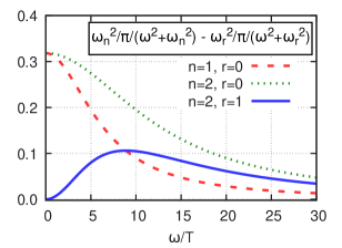
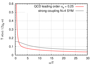
Figure 1: Left: The integration kernels of Eqs. (12) and (13) multiplying the function $\sigma(\omega)/\omega$. Right: The spectral function normalized by $2\chi_{s}\omega/T$ at lightlike kinematics in QCD at complete leading order according to Ref. Arnold et al. (2001b, a), and in the strongly-coupled $\mathcal{N}=4$ SYM theory Caron-Huot et al. (2006b).

II.2 Lattice subtractions

The lattice regulator breaks Lorentz symmetry: short-distance contributions to $H_{E}(\omega_{n})$ emerge which would hamper the continuum extrapolation. It is therefore necessary to develop suitable lattice representations of $H_{E}(\omega_{n})$. In fact, for discretizations of the correlator which use two local currents or two exactly-conserved lattice currents, such subtractions are required to cancel divergences arising from contact terms and have a well-defined continuum limit, see Sec. II.4 for further discussion. This can be achieved in several ways, for instance by subtracting the vacuum lattice correlator obtained at the same bare parameters, as was proposed in Ref. Meyer (2018) or by subtracting a thermal correlator having the same short-distance properties Meyer et al. (2022).

The basic observation is that the Fourier-transform of a static screening correlator at lightlike momentum vanishes in the continuum. Indeed, the restriction of the polarisation tensor to spatial components in the static sector has the form

$$\Pi_{ij}(\mathbb{p})\equiv\int_{0}^{\beta}\mathrm{d}x_{0}\int\mathrm{d}^{3}x\;e^{i\mathbb{p}\mathbb{x}}\;\langle J_{i}(x)\,J_{j}(0)\rangle=(p_{i}p_{j}-\delta_{ij}\mathbb{p}^{2})\Pi(\mathbb{p}^{2})$$ (16)

familiar from the vacuum polarisation. From here and from the absence of a pole in $\Pi$ at $\mathbb{p}^{2}=0$ follows immediately the property

$$\int_{-\infty}^{\,\infty}\mathrm{d}x_{3}\;{G^{\mathrm{T}}_{\rm{st}}(p,x_{3})}\;\mathrm{e}^{-px_{3}}=0,\quad\forall p\in\mathbb{R}.$$ (17)

Thus, generalizing the estimator proposed in Meyer et al. (2022), we consider a subtraction involving the static screening correlator at momentum $p$,

$$H_{E,\,p}(\omega_{n}) =-\int_{0}^{\beta}\mathrm{d}x_{0}\int\mathrm{d}^{3}x\,\left({\mathrm{e}^{\omega_{n}\,(\mathrm{i}x_{0}-x_{3})}}-{\mathrm{e}^{p\,(\mathrm{i}x_{2}-x_{3})}}\right)\,\langle J_{1}(x)J_{1}(0)\rangle$$

$$=\int_{-\infty}^{\,\infty}\mathrm{d}x_{3}\,\Big{[}{G^{\mathrm{T}}_{\rm{ns}}(\omega_{n},x_{3})}\mathrm{e}^{-\omega_{n}x_{3}}-{G^{\mathrm{T}}_{\rm{st}}(p,x_{3})}\mathrm{e}^{-px_{3}}\Big{]}\,.$$ (18)

We note again that in the case of the static (st) transverse channel screening correlator (defined in Eq. (7)), the momentum $p$ is inserted into a spatial direction (here $x_{2}$) orthogonal to $x_{3}$ and to the directions corresponding to the Lorentz indices of the currents (here $x_{1}$). The case of $p=\omega_{n}$ Meyer et al. (2022) has the special property that $H_{E,\,\omega_{n}}(\omega_{n})$ vanishes identically at $T=0$, correctly reproducing the continuum property that $H_{E}(\omega_{n})$ vanishes in the vacuum. This property is expected to reduce discretisation errors of $H_{E,\,\omega_{n}}(\omega_{n})$ at non-zero temperature, an expectation that is confirmed in lattice perturbation theory (see App. E).

We remark that even more general subtractions

$$H_{E,\,{\bf p},\,{\bm{\alpha}}}(\omega_{n})=\int_{-\infty}^{\infty}\mathrm{d}x_{3}\Big{[}G_{\rm{ns}}^{\mathrm{T}}(\omega_{n},x_{3})\mathrm{e}^{-\omega_{n}x_{3}}-\sum_{i}\alpha_{i}G_{\rm{st}}^{\mathrm{T}}(p_{i},x_{3})\mathrm{e}^{-p_{i}x_{3}}\Big{]}$$ (19)

are possible, i.e. one can subtract a general linear combination of static screening correlators at different values of $p_{i}$. Eq. (18) is a special case of Eq. (19) with $\alpha_{1}=1$, $p_{1}=p$ and $\alpha_{i>1}=0$. When evaluated at different values of $p$, the results for $H_{E,\,p}(\omega_{n})$ in Eq. (18) do not agree with each other in general on a finite lattice, but they have to match after taking the continuum limit. The same holds for the quantity in Eq. (19), i.e. choosing different $\alpha_{i}$ coefficients and subtracting the static screening correlators evaluated at different momenta, the results for $H_{E,\,{\bf p},\,\bm{\alpha}}(\omega_{n})$ differ at a finite lattice spacing, but have to agree in the continuum. One can exploit these observations and propose subtractions that may have more tractable integrands and/or reduced cutoff effects toward the continuum.

Similarly, a direct probe of the difference of $H_{E}(\omega_{n})$ and $H_{E}(\omega_{r})$ on the lattice is provided by the discretized version of

$$[H_{E}(\omega_{n})-\varepsilon H_{E}(\omega_{r})]_{{\bf p},\,\bm{\alpha}}=\int_{-\infty}^{\infty}\mathrm{d}x_{3}\Big{[}G_{\rm{ns}}^{\mathrm{T}}(\omega_{n},x_{3})\mathrm{e}^{-\omega_{n}x_{3}} -\varepsilon\,G_{\rm{ns}}^{\mathrm{T}}(\omega_{r},x_{3})\mathrm{e}^{-\omega_{r}x_{3}}$$

$$-\sum_{i}\alpha_{i}G_{\rm{st}}^{\mathrm{T}}(p_{i},x_{3})\mathrm{e}^{-p_{i}x_{3}}\Big{]}.$$ (20)

Again, the contribution coming from the static screening correlators in Eq. (20) vanishes in the continuum.

We will explicitly investigate the more general subtracions for the extraction of $H_{E}(\omega_{2})$, i.e. in the second Matsubara sector, as well as for the difference $H_{E}(\omega_{2})-H_{E}(\omega_{1})$ in Sec. IV. Additionally, alternative subtractions concerning $H_{E}(\omega_{1})$ and $H_{E}(\omega_{2})$ will be exploited in Apps. B and C, respectively. In the rest of the paper we use the notation $H_{E}$ omitting the extra subscripts to indicate the standard subtraction with $\alpha_{1}=1$, $\alpha_{i>1}=0$ and $p=p_{1}=\omega_{n}$.

II.3 Probing the virtuality dependence of $H_{E}$

Until this point, the above discussion focused on observables at vanishing virtuality, since this is the relevant kinematics for the photon emissivity. We note that $H_{E}$ can also be evaluated for a given non-vanishing virtuality, which can be helpful to understand the behavior of the low-mass dilepton rate Cè et al. (2021a). In order to investigate the effect of introducing a small non-vanishing $Q^{2}$, we can calculate the derivative of $H_{E}$ with respect to $Q^{2}$, evaluated at $Q^{2}=0$. For that, we start from the definition given in Ref. Cè et al. (2021a)

$$H_{E}(\omega_{n},Q^{2}) =-\int_{0}^{\beta}\mathrm{d}x_{0}\,\int\mathrm{d}^{3}x\,\,\mathrm{e}^{\mathrm{i}\omega_{n}x_{0}}\,\,\mathrm{e}^{\sqrt{\omega_{n}^{2}-Q^{2}}x_{3}}\,\,\langle J_{1}(x)J_{1}(0)\rangle$$

$$=\int_{-\infty}^{\infty}\mathrm{d}x_{3}\,G^{\mathrm{T}}_{E,{\rm ns}}(\omega_{n},x_{3})\,\,\mathrm{e}^{\sqrt{\omega_{n}^{2}-Q^{2}}x_{3}}.$$ (21)

By expanding around $Q^{2}=0$ for $\omega_{n}>0$ we obtain

$$H_{E}(\omega_{n},Q^{2}) =H_{E}(\omega_{n},0)+Q^{2}\,\Bigg{[}\frac{\mathrm{d}H_{E}(\omega_{n},Q^{2})}{\mathrm{d}Q^{2}}\Bigg{]}_{Q^{2}=0}+\mathcal{O}(Q^{4})$$

$$=H_{E}(\omega_{n},0)-\frac{Q^{2}}{2\omega_{n}}\int_{-\infty}^{\infty}\mathrm{d}x_{3}\,\,x_{3}\,\,G^{\mathrm{T}}_{E,{\rm ns}}(\omega_{n},x_{3})\,\,\mathrm{e}^{\omega_{n}x_{3}}+\mathcal{O}(Q^{4}).$$ (22)

Evaluating the derivative in the free theory, we can use the asymptotic formula $G^{\mathrm{T}}_{E,{\rm ns}}(\omega_{n},x_{3})\overset{x_{3}\to\infty}{\sim}\,\mathrm{e}^{-\omega_{n}|x_{3}|}/x_{3}^{2}$ (see Ref. Brandt et al. (2014), Eq. (3.11)). With this we find that in the free theory, the $\mathcal{O}(Q^{2})$ term contains an infrared-divergent term,

$$H_{E}(\omega_{n},Q^{2})=H_{E}(\omega_{n},0)+c_{n}\,Q^{2}\log(Q^{2}/\omega_{n}^{2})+\mathcal{O}({Q^{2}})$$ (23)

with $c_{1}=N_{c}/(32\pi^{2})$. This coefficient can be obtained by introducing a cutoff $1/Q$ for the $x_{3}$-integral.

In order to ensure that we have a definition that is ultraviolet-finite, we remove the divergence present at finite $Q^{2}$ by subtracting $H_{E}(0,Q^{2})$, which does not change the value at $Q^{2}=0$ of the function we are Taylor-expanding because $H_{E}(0,0)=0$. Thus we evaluate

$$\frac{\mathrm{d}}{\mathrm{d}Q^{2}}\left[H_{E}(\omega_{n},Q^{2})-H_{E}(0,Q^{2})\right]_{Q^{2}=0} =-\int_{0}^{\infty}\mathrm{d}x_{3}\,\left[\frac{x_{3}}{\omega_{n}}\sinh(\omega_{n}x_{3})G^{\mathrm{T}}_{{\rm ns}}(\omega_{n},x_{3})-x_{3}^{2}G^{\rm T}_{\rm st}(0,x_{3})\right].$$ (24)

In Eq. (24), $G_{\rm st}^{\mathrm{T}}(0,x_{3})$, which denotes the static, zero-momentum screening correlator, does not yield an infrared-enhanced contribution.

II.4 Lattice observables

In this Section, we introduce the lattice observables that we have investigated. We define the bare local and the conserved vector current as

$$V_{\mu}^{\mathrm{L}}(x)=\widebar{\Psi}(x)\frac{\tau_{3}}{\sqrt{2}}\gamma_{\mu}\Psi(x),$$ (25)

and

$$V_{\mu}^{\mathrm{C}}(x)=\frac{1}{2}\left[\widebar{\Psi}(x+a\hat{\mu})(1+\gamma_{\mu})U^{\dagger}_{\mu}(x)\frac{\tau_{3}}{\sqrt{2}}\Psi(x)-\widebar{\Psi}(x)(1-\gamma_{\mu})U_{\mu}(x)\frac{\tau_{3}}{\sqrt{2}}\Psi(x+a\hat{\mu})\right],$$ (26)

respectively, where $\Psi=(u,d)^{\top}$ represents the isospin doublet of mass-degenerate quark fields and $\tau_{3}$ is the diagonal Pauli matrix. In other words, we focus on the isovector flavour combination, the current being normalized according to $\sum_{f}Q_{f}^{2}=1$. It is in that normalization that our results for $H_{E}(\omega_{n})$ are given. For an estimate of the physical photon emissivity assuming SU(3) flavour symmetry among the $(u,d,s)$ quarks, one must include the factor $\sum_{f}Q_{f}^{2}=(2/3)^{2}+(-1/3)^{2}+(-1/3)^{2}=2/3$.

Using Eqs. (25) and (26), we define the following bare, non-static screening correlators:

$$G^{\alpha\beta}_{{\rm ns},\,\mu\nu}(\omega_{n},x_{i})=-a^{3}\sum_{\begin{subarray}{c}x_{j}\\ j\in\{0,1,2,3\},\,j\neq i\end{subarray}}\mathrm{e}^{\mathrm{i}\omega_{n}x_{0}}\,\langle V_{\mu}^{\alpha}(x)V_{\nu}^{\beta}(0)\rangle,\qquad i\in\{1,2,3\},\qquad\alpha,\beta\in\{L,C\}$$ (27)

The Greek letters $\alpha$ and $\beta$ stand for the discretization of the current at sink and source, respectively. We call the above correlators non-static, because the momentum is inserted into the Euclidean time-direction. We denote these with the subscript ${\rm ns}$. By contrast, when injecting the momentum into a spatial direction, $k$, – perpendicular to direction of $x_{i}$ –, we got the bare, static screening correlators at finite momentum,

$$G^{\alpha\beta}_{{\rm st},\,\mu\nu}(\omega_{n},x_{i})=-a^{3}\sum_{\begin{subarray}{c}x_{j}\\ j\in\{0,1,2,3\},\,j\neq i\end{subarray}}\mathrm{e}^{\mathrm{i}\omega_{n}x_{k}}\,\langle V_{\mu}^{\alpha}(x)V_{\nu}^{\beta}(0)\rangle,\quad i,k\in\{1,2,3\},\,\quad i\neq k,\quad\alpha,\beta\in\{L,C\}.$$ (28)

After choosing a particular spatial decay direction (direction of the correlator separation), $i$, we obtain the screening correlators in the transverse channel by choosing $\mu=\nu$ orthogonal to this decay direction. We note here that we do not discriminate the notation used for the continuum or the lattice observables, i.e. we use capital $G$ for the lattice and for the continuum screening correlators as well.

We also specify the correlator at a momentum transverse to both $\mu=\nu$ and $i$. Therefore, we have in total six possible combinations of the decay direction and of the Lorentz indices of the currents for the non-static screening correlator and also six combinations of the decay direction, the Lorentz indices of the currents and the momentum inserted for the static screening correlator. We average over these different screening correlators measured on the same configuration. Moreover, the local-conserved and conserved-local discretizations can be transformed into each other, using Cartesian coordinate reflections. Therefore, we average these two and refer to this averaged correlator with the superscript LC in the following. We renormalize the correlators by multiplying by $Z_{V}(g_{0}^{2})$ whenever the local vector current is included using the vector current renormalization constant from Ref. Dalla Brida et al. (2019). Instead of the electromagnetic current, we use the isovector vector current whereby disconnected contributions are absent.

As mentioned already at the beginning of Sec. II.2, one has to pay special attention when formulating a lattice estimator for $H_{E}$, since a naive implementation of Eq. (11) on the lattice, could lead to ultraviolet divergences. A crucial point at small separation $x$ is the removal of the $x$-independent part multiplying the expectation value of the product of currents in Eq. (11). The simplest way of doing this is to subtract the static screening correlator at vanishing momentum, or to subtract it evaluated at the same finite momentum $\omega_{n}$,

$$H_{E}^{\rm(sub)}(\omega_{n})/T^{2}=\frac{a}{L_{t}}\sum_{x_{3}=a}^{L_{s}/2-a}h(\omega_{n},x_{3})+\frac{a}{2L_{t}}\Big{(}h(\omega_{n},0)+h(\omega_{n},L_{s}/2)\Big{)}$$ (29)

where we used the trapezoid formula when discretizing Eq. (18) with $p=\omega_{n}$ and $L_{t}$ ($L_{s}$) stands for the temporal (spatial) size of the lattice. The lattice spacing is deenoted by $a$ and $h(\omega_{n},x_{3})$ is the integrand,

$$h(\omega_{n},x_{3})=\frac{2}{T^{3}}\Big{(}G_{\rm ns}^{\mathrm{T}}(\omega_{n},x_{3})-G_{\rm st}^{\mathrm{T}}(\omega_{n},x_{3})\Big{)}\cosh(\omega_{n}x_{3}).$$ (30)

We note that $G^{\mathrm{T}}_{\rm ns}$ as well as $G^{\mathrm{T}}_{\rm st}$ are negative in our conventions and since in absolute value we found $G^{\mathrm{T}}_{\rm ns}$ larger than $G^{\mathrm{T}}_{\rm st}$, $H_{E}^{\rm(sub)}(\omega_{n})/T^{2}$ will also be negative. From now on we leave the (sub) superscript from $H_{E}^{\rm(sub)}(\omega_{n})$, and similarly to the correlators, we do not discriminate between the continuum and lattice observables, i.e. we use the same symbol.

Analogously as in the case of $H_{E}(\omega_{n})$, one can obtain the lattice formula for the derivative of $H_{E}(\omega_{n},Q^{2})$ w.r.t. $Q^{2}$ by applying the trapezoid formula to Eq. (24), but where $h(\omega_{n},x_{3})$ of the right-hand side of Eq. (29) is replaced by

$$h_{Q^{2}}(\omega_{n},x_{3})=-\frac{1}{T^{3}}\Big{(}\,\frac{x_{3}T}{\omega_{n}/T}\,\sinh(\omega_{n}x_{3})\,G^{\mathrm{T}}_{\rm{ns}}(\omega_{n},x_{3})-(x_{3}T)^{2}G^{\mathrm{T}}_{\rm{st}}(0,x_{3})\Big{)}.$$ (31)

We note that this subtraction involves the completely static — zero-momentum — screening correlator, $G_{\rm{st}}^{\mathrm{T}}(p=0,x_{3})$.

II.5 Simulation details

To calculate the screening correlators which enter the expression (29) for $H_{E}$, we used three ensembles generated at the same temperature $T\sim 250$ MeV in the high-temperature phase. We employ two-flavor O($a$)-improved dynamical Wilson fermions and the plaquette gauge action; further details regarding the lattice action we used can be found in Ref. Fritzsch et al. (2012). The configurations for the W7 ensemble have been generated using the openQCD-1.6 package and the ones of O7 and most of those of X7 using openQCD-2.0 Luscher and Schaefer (2013). 512 configurations of the X7 ensemble were generated using the MP-HMC algorithm Hasenbusch (2001) in the implementation described in Ref. Marinkovic and Schaefer (2010). The pion mass in the vacuum is around $m_{\pi}\approx 270$ MeV Fritzsch et al. (2012); Engel et al. (2015), and the lattice spacings are in the range of 0.033–0.05 fm Fritzsch et al. (2012); Cè et al. (2021b). The boundary conditions are periodic in space, while those in the time direction are periodic for the gauge field and antiperiodic for the quark fields, as required by the Matsubara formalism.

label	$6/g_{0}^{2}$	$\kappa$	$L_{t}/a$	$N_{\rm conf}$	$\frac{\rm MDUs}{\rm conf\phantom{{}_{A}}}$
O7	5.5	0.13671	16	1500	20
W7	5.685727	0.136684	20	1600	8
X7	5.827160	0.136544	24	2012	10

Table 1: Overview of the $N_{f}=2$ ensembles used in this study. Simulations were carried out at a fixed temperature of $T\approx 254\,$MeV and fixed aspect ratio $L_{s}/L_{t}=4$, where $L_{s}$ ($L_{t}$) is the spatial (temporal) linear size of the lattice. The parameters given are the bare gauge coupling $g_{0}$, the Wilson hopping parameter $\kappa$, the temporal size in units of the lattice spacing $a$, the number of configurations used $N_{\rm conf}$ and the number of molecular-dynamics time units (MDUs) separating these configurations. The number of point sources per configuration is 64 in all cases.

III Results

III.1 The integrand for obtaining $H_{E}$

As we have shown in Sec. II.4, the crucial ingredients for calculating $H_{E}$ through Eq. (29) are the non-static and static transverse screening correlators at finite spatial momentum. These have been first investigated in detail in weak-coupling theory complemented with lattice QCD simulations on a single ensemble in Ref. Brandt et al. (2014). In that work, however, the static screening correlators have been studied only at vanishing momentum.

For the determination of $H_{E}$, we first analyzed the screening correlators measured on the three ensembles. We discarded a few outliers from the dataset (see App. A) and estimated the statistical errors using jackknife resampling with 200 jackknife samples. Then we formed the integrand (see Eq. (30)), which is shown in Fig. 2 for our finest ensemble.

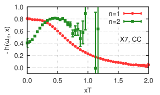
Figure 2: The integrand (Eq. (30)) for the calculation of $H_{E}(\omega_{n})$ on our finest ensemble X7, using the conserved-conserved discretization of the current-current correlator.

As Fig. 2 shows, the quantity $H_{E}(\omega_{1})$ receives dominant contributions from the $xT\lesssim 1-1.5$ region and with the present statistics, we have good control over the signal. The relative error on the integrand for $H_{E}(\omega_{1})$ is below 1% for $xT\lesssim 1.1$ on the finest ensemble shown in Fig. 2. However, trying to evaluate $H_{E}$ in the $n=2$ Matsubara sector reveals that one faces a severe, exponential signal-to-noise problem. The variances on the non-static correlator values are an order of magnitude larger in the $n=2$ sector than for $n=1$, and multiplying by $\cosh(2\pi Tn)$ makes the situation even worse. Therefore, we focus first on evaluating $H_{E}$ in the $n=1$ Matsubara sector and return to $n=2$ only in Secs. IV.1 and  IV.2.

III.2 Modelling the tail of the screening correlators

While the dominant contribution to $H_{E}(\omega_{1})$ comes from short distances, the long-distance contribution is also non-negligible. However, it is noisier, because the screening correlators are less precise at large distances and the difference is less smooth than for short distances. Directly performing the sum of Eq. (29) for $H_{E}(\omega_{1})$ results in having relative errors of about $1.37,1.50,1.90\%$ for the LL, LC and CC discretizations, respectively, on our coarsest and also ‘noisiest’ ensemble. We aim at a more precise determination of $H_{E}(\omega_{1})$ and as we will see in this section, by proper handling of the tail these errors could be reduced to $0.91,0.77,1.03\%$, respectively.

Moreover, we have an exponentially growing weight function multiplying the difference of the correlators and this results in a small enhancement of the integrand in the region $x_{3}\sim L/2$. This effect is the consequence of calculating the integrand in a finite volume. In order to correct for it, we applied a simple model based on fits on the screening correlators to describe the tail of the integrand. This way we have better control over the long-distance contribution and also we could correct for finite volume effects. We use the fact, that the non-static screening correlators have a representation in terms of energies and amplitudes of screening states in the following form Meyer (2018):

$$G_{\rm{ns}}(\omega_{r},x)\overset{x\neq 0}{=}\sum_{n=0}^{\infty}|A_{\rm{ns},n}^{(r)}|^{2}\mathrm{e}^{-E_{\rm{ns},n}^{(r)}|x|}.$$ (32)

A similar expression holds for the static correlator:

$$G_{\rm{st}}(\omega_{r},x)\overset{x\neq 0}{=}\sum_{n=0}^{\infty}|A_{\rm{st},n}^{(r)}|^{2}\mathrm{e}^{-E_{\rm{st},n}^{(r)}|x|}.$$ (33)

The low-lying screening spectrum can be studied using weak-coupling methods as well Brandt et al. (2014). The lowest energy of a screening state in a given Matsubara sector with frequency $\omega_{r}$ is often called the screening mass and is denoted by $E^{(r)}_{0}$. In this section, we consider only the first Matsubara sector, $\omega_{1}=2\pi T$, therefore in the following we do not write out explicitly the momentum dependence.

Using the above formulae, our procedure to get a better handle over the integrand is the following:

1. We split the integrand, $h(x)\equiv h(\omega_{1},x)$ (c.f. Eq. (30)) into two parts

   $$h(x)=h(x)(1-\Theta(x,x_{w},\Delta))+h(x)\Theta(x,x_{w},\Delta)$$ (34)

   using a smooth step function,

   $$\Theta(x,x_{w},\Delta)=(1+\tanh[(x-x_{w})/\Delta])/2.$$ (35)

   We call the first term in Eq. (34) the short-distance and the second term the long-distance part of the integrand.

2. We integrate the short-distance contribution using the trapezoidal formula.

3. We perform single-state fits on the tails of the screening correlators using the representations given in Eqs. (32) and (33) translated to a form corresponding to a periodic lattice, namely

   $$G^{\rm{(ns)}}_{\rm{ansatz}}(x)=|A_{\rm{ns},0}|^{2}\cosh[E_{\rm{ns},0}(x-L_{s}/2)\big{]}$$ (36)

   and

   $$G^{\rm{(st)}}_{\rm{ansatz}}(x)=|A_{\rm{st},0}|^{2}\cosh[E_{\rm{st},0}(x-L_{s}/2)\big{]},$$ (37)

   for the non-static and for the static screening correlators, respectively. In Eqs. (36) and (37), $L_{s}$ is the spatial length of the lattice.

4. Using the fit results $A_{\rm{ns},0}$ and $E_{\rm{ns},0}$ as well as $A_{\rm{st},0}$ and $E_{\rm{st},0}$, we replace the long-distance part of Eq. (34) by the corresponding infinite volume formula:

   $$h_{\rm{ansatz,iv}}(x)\Theta(x,x_{w},\Delta) =\Big{[}|A_{\rm{ns},0}|^{2}\frac{\mathrm{e}^{E_{\rm{ns},0}L_{s}/2}}{2}\Big{(}\mathrm{e}^{-(E_{\rm{ns},0}+\omega_{1})x}+\mathrm{e}^{-(E_{\rm{ns},0}-\omega_{1})x}\Big{)}$$

   $$-|A_{\rm{st},0}|^{2}\frac{\mathrm{e}^{E_{\rm{st},0}L_{s}/2}}{2}\Big{(}\mathrm{e}^{-(E_{\rm{st},0}+\omega_{1})x}+\mathrm{e}^{-(E_{\rm{st},0}-\omega_{1})x}\Big{)}\Big{]}\Theta(x,x_{w},\Delta).$$ (38)

   This we can integrate analytically using:

   $$\int\mathrm{d}x\,\mathrm{e}^{-\alpha_{1}x}\tanh(x-\alpha_{2})=\frac{1}{\alpha_{1}}\mathrm{e}^{-\alpha_{1}x}\Big{(}2{}_{2}F_{1}(1,-\alpha_{1}/2;1-\alpha_{1}/2;-\mathrm{e}^{2x-2\alpha_{2}})-1\Big{)}+\rm{const},$$ (39)

   where ${}_{2}F_{1}$ denotes the hypergeometric function.

While the single-state fits describe the actual data well, i.e. with good $\chi^{2}$ and p-values, we note that the identification of the plateau region was not clear in some cases, although we performed a thorough scan using all possible fit ranges having different starting points and different lengths with 6$a$–11$a$. Therefore, we also made an attempt to fit the data with two-state fits with or without using priors from weak-coupling theory (c.f. Sec. F), but these fit results were not satisfactory. Typically on the coarsest or the coarser two ensembles, they either failed to describe the data, gave too large errors or returned a near-zero or negative $|A|^{2}$ coefficient — which we did not constrain — for the excited state. When the two-state fits were able to describe the data well, the ground-state static screening energy they returned was too small — as we could deduce it using the zero-momentum correlators. Therefore we decided to stick to single-state fits.

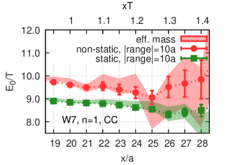
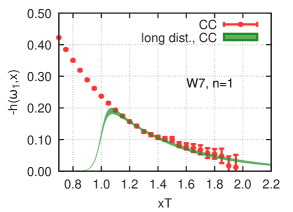
Figure 3: Left: fitted masses, with circles and squares corresponding to $G_{\rm ns}^{\mathrm{T}}(\omega_{1},x_{3})$ and $G_{\rm st}^{\mathrm{T}}(\omega_{1},x_{3})$ respectively, using a fit range of ten lattice spacings. The bands represent the ’cosh’ effective masses. Right: the tail of the integrand needed for the calculation of $H_{E}$ at the first Matsubara frequency. The red points are the actual datapoints on our second coarsest lattice and the band shows the result of the modelling.

Besides fitting, we also determined the effective mass using two consecutive correlator datapoints, by solving the algebraic equation

$$\frac{G(x+a)}{G(x)}=\frac{\cosh[m_{\rm{eff}}(x+a-L_{s}/2)\big{]}}{\cosh[m_{\rm{eff}}(x-L_{s}/2)\big{]}}$$ (40)

for $m_{\rm{eff}}$. Here, $G(x)$ denotes the actual lattice data for the non-static or the static screening correlators. We found that the effective masses are in quite good agreement with the fitted masses, but also do not show a clear and long plateau as $x$ increases, see Fig. 3, left panel. Therefore, instead of fitting a constant, we decided to choose three representatives from a histogram built by assigning Akaike-weights Akaike (1971); Borsanyi et al. (2021) to all the fitted masses that we obtained in the most plateau-like region. In all cases, we chose a wide region, before the noise gets too large on the fitted masses. For instance for the W7 ensemble, we choose fit results on conserved-conserved correlator data in the range from $x/a=21$ to 25 for both correlators (left panel of Fig. 3). We propagate the median as well as the values near the 16th and 84th percentiles of the histograms to the later steps of the analysis of $H_{E}(\omega_{1})$.

III.3 Continuum extrapolation of $H_{E}(\omega_{1})$

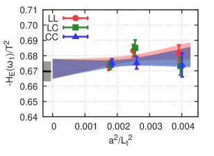
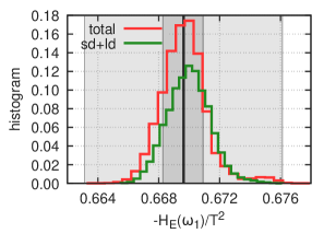
Figure 4: Left: A representative continuum limit of $-H_{E}(\omega_{1})/T^{2}$ obtained from Eqs. (29–30). Right: AIC-weighted histogram of the continuum extrapolated results for $-H_{E}(\omega_{1})/T^{2}$ obtained with $x_{w}T=1.1$. The AIC-weighted histogram of the long-distance contribution to $H_{E}(\omega_{1})$, shifted with the continuum result for the short-distance contribution, is also shown for comparison (sd+ld). The dark-grey band shows the systematic error, and the lighter gray band represents the total error obtained from the statistical and systematic errors added in quadrature.

As we described in Sec. III.2, we used single-state fits to describe the tail of the non-static and static screening correlators and for each ensemble and discretization we built a histogram of the fit results from the plateau region, from which we chose three representatives. When proceeding this way for each correlators, we obtain $3\times 3=9$ possibilities for modelling the tail of the integrand, Eq. (38), for a given ensemble and a given discretization. We calculated $H_{E}$ using all these nine combinations for the tail, sorted the results and then chose the median, the values near the 16th and near the 84th percentile after assigning uniform weights for these slightly different values of $H_{E}$.

This way we had three representative values of $H_{E}$ for each ensemble and discretization that went into the next step of the analysis, which was the continuum extrapolation. We used these in all possible combinations when performing a correlated simultaneous continuum extrapolation using a linear ansatz in $a^{2}$. These gave $(3^{3})^{3}=19683$ different continuum extrapolations. We make further variations by omitting one of the coarsest datapoints from the extrapolation, which also lead to $3^{3}\cdot 3^{3}\cdot(3^{2}\cdot 3)=19683$ different continuum extrapolations. We then built an AIC-weighted histogram from using all $2\cdot 19683$ continuum extrapolations to estimate the systematic error. A representative continuum extrapolation as well as the AIC-weighted histogram are shown in Fig. 4, left and right panel, respectively.

The transition to the modelled tail has been introduced smoothly by using a smooth step function of Eq. (35) and we investigated the effect of choosing different switching points, $x_{w}$, in the range $x_{w}T$=0.9–1.3. We found that the results were stable against these choices, see Fig. 5.

Our final result for $H_{E}$ in the first Matsubara sector is

$$H_{E}(\omega_{1})/T^{2}=-0.670(6)_{\rm{stat}}(1)_{\rm{sys}}.$$ (41)

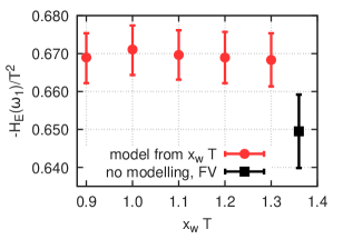
Figure 5: Comparison of continuum results for $-H_{E}(\omega_{1})/T^{2}$ using different starting points for the modelling.

III.4 Continuum extrapolation of the $Q^{2}$-derivative of $H_{E}(\omega_{1},Q^{2})$ at $Q^{2}=0$

In order to retrieve information about the $Q^{2}$-dependence of our observable, we evaluate the $Q^{2}$-derivative of the difference, $H_{E}(\omega_{1},Q^{2})-H_{E}(0,Q^{2})$, as it was discussed in Sec. II.3. The continuum observable is defined in Eq. (24), and the corresponding integrand on the lattice is introduced in Eq. (31). It is interesting to have a look on this integrand — left panel of Fig. 6 — which is more pronounced at short distances than the integrand $h(\omega_{1},x)$, that we had shown for $H_{E}(\omega_{1})$ in Fig. 2. It starts from zero quadratically in $x$, and after having a peak, it crosses zero around $xT\sim 1$, but the long-distance contribution is much more suppressed than it was for $H_{E}(\omega_{1})$.

For the continuum extrapolation we applied a similar proceduce as for $H_{E}(\omega_{1})$ discussed in Sec. III.3. Our final continuum estimate is

$$\frac{\mathrm{d}}{\mathrm{d}Q^{2}}\left[H_{E}(\omega_{n},Q^{2})-H_{E}(0,Q^{2})\right]_{Q^{2}=0}=-0.0282(4)_{\rm{stat}}(1)_{\rm{sys}}.$$ (42)

We remark that the result is on the order of $-N_{c}/(2\pi)^{2}$ and does not exhibit any strong infrared enhancement as would be expected at very weak coupling (see Eq. (23)).

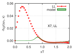
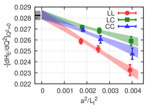
Figure 6: Left: The integrand, $h_{Q^{2}}(\omega_{1},x)$, defined in Eq. (31) for the derivative of $H_{E}(\omega_{1},Q^{2})$ with respect to $Q^{2}$ at $Q^{2}=0$. Right: Representative continuum extrapolation of $\mathrm{d}[H_{E}(\omega_{1},Q^{2})-H_{E}(0,Q^{2})]/\mathrm{d}Q^{2}$ at $Q^{2}=0$.

III.5 Continuum extrapolation of the screening masses

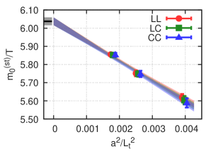
Figure 7: Continuum extrapolation of the static screening mass obtained using the screening correlator at vanishing momentum.

As we have already mentioned in Sec. II.1, the screening masses extracted from the correlators we investigate here can also be determined using weak-coupling theory. The first relevant study in this direction was Ref. Brandt et al. (2014), which also compared the leading-order (LO) and next-to-leading order (NLO) screening masses to lattice results. However, Ref. Brandt et al. (2014) investigated only screening correlators at finite temporal or at vanishing momentum. Moreover, the lattice investigation has used only coarse ensembles without taking the continuum limit.

In this work, we extend this first investigation in several aspects: we investigate also screening masses obtained from screening correlators at finite spatial momentum besides the ones obtained at finite temporal or at vanishing momentum. We accumulated much more configurations and performed more measurements, enabling us to improve the signal-to-noise ratio at the tails of the correlators. Finally, we also extrapolate our results to the continuum using three ensembles, from which the finest has a lattice spacing about 2/3 the lattice spacing of Ref. Brandt et al. (2014).

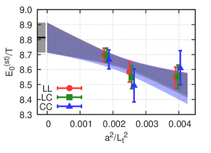
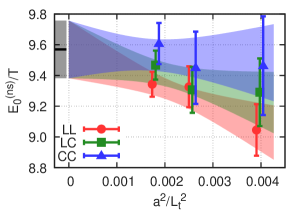
Figure 8: Continuum extrapolation of the lowest screening mass associated with the correlators $G^{\mathrm{T}}_{\rm st}(\omega_{1},x_{3})$ and $G^{\mathrm{T}}_{\rm ns}(\omega_{1},x_{3})$, left and right panel, respectively.

We start by discussing the zero and finite spatial momentum results. We performed single-state fits — discussed also in Sec. III.2 — using the fit ansatz given in Eq. (37). The screening correlators at vanishing momentum are more precise above $xT\sim 1.2$ than at the first spatial Matsubara momentum, making it possible to determine the screening masses at 0.15–0.45% precision depending on the ensembles and discretizations. By using the dispersion relation, we could compare the extracted masses at vanishing momentum to those at momentum $2\pi T$. With this comparison, we observe that the screening masses determinded via the dispersion relation, $\sqrt{m_{0}^{(\rm{st})\,2}+(2\pi T)^{2}}$, give a slightly smaller value than the corresponding result at the first Matsubara momentum.

Since the single-state fitting procedure starting at later and later datapoints provides fit results converging to an asymptotic value more reliably than in the cases with finite momentum and the errors are comparable in the plateau region, we chose only one representative for each ensemble and discretization and performed the continuum extrapolation linear in $a^{2}$ using that. We also assigned a systematic error to the continuum extrapolation by removing one of the discretizations on the coarsest ensemble. The continuum extrapolation using all datapoints is shown in Fig. 7. Our continuum estimate having about 0.37% error is

$$m_{0}^{(\rm st)}/T=6.04(2)_{\rm{stat}}(1)_{\rm{sys}}.$$ (43)

Using this result and the dispersion relation, an estimate for static screening mass at (spatial) momentum $\omega_{1}=2\pi T$ is

$$E_{0,\rm{dr}}^{\rm{(st)}}/T=\sqrt{(m_{0}^{\rm(st)}/T)^{2}+(2\pi)^{2}}=8.72(2)_{\rm{stat}}(1)_{\rm{sys}}.$$ (44)

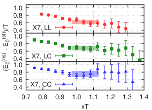
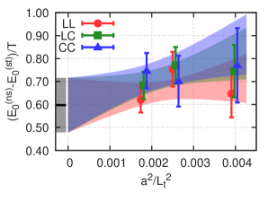
Figure 9: Left: Fit results for the gap between the ground-state non-static and static screening masses, respectively associated with the correlators $G_{\rm ns}^{\mathrm{T}}(\omega_{1},x_{3})$ $G_{\rm st}^{\mathrm{T}}(\omega_{1},x_{3})$, and the window-smeared results shown by the bands. Right: Continuum extrapolation of the difference of the ground-state non-static and static screening masses.

The static screening masses being directly available at this momentum, we can extrapolate those to the continuum and see how close we get to the estimate given in Eq. (44). Therefore, we calculated a weighted average of the masses obtained by fitting the static screening correlator. We performed the averaging using the difference of smooth step functions — introduced in Eq. (35) — with parameters $x_{w}T=0.975$ and $x_{w}T=1.125$, i.e. the averaging window has a width about 0.15 and was centered at 1.05. $T\Delta$ was chosen to be 0.01. We made similar variations as before, leaving out one datapoint from the coarsest ensemble and arrived at the continuum estimate:

$$E_{0}^{\rm{(st)}}/T=8.81(10)_{\rm{stat}}(2)_{\rm{sys}}$$ (45)

The continuum extrapolation is shown in the left panel of Fig. 8. The result in Eq. (45) is in good agreement with the estimate based on using the $n=0$ screening mass and the dispersion relation, Eq. (44).

Using the same procedure for the continuum extrapolation of the non-static screening mass as in the case of the static, we obtained the following result in the first Matsubara sector:

$$E_{0}^{\rm{(ns)}}/T=9.57(19)_{\rm{stat}}(11)_{\rm{sys}}.$$ (46)

The continuum extrapolation is shown in the right panel of Fig. 8.

As a crosscheck, we also investigated the possibility of determining the non-static screening mass using the ratio of the non-static and static screening correlators. By making use of the following approximate formula,

$$\frac{|A_{n}^{\rm{(ns)}}|^{2}}{|A_{n}^{\rm{(st)}}|^{2}}\frac{\cosh[E_{0}^{\rm{(ns)}}(x-L/2)]}{\cosh[E_{0}^{\rm{(st)}}(x-L/2)]}\approx C\mathrm{e}^{-(E_{0}^{\rm{(ns)}}-E_{0}^{\rm{(st)}})x},\quad(x\ll L/2),$$ (47)

we fitted the ratio of the correlators using the ansatz on the right-hand side of this equation. After performing the averaging over the obtained differences $(E_{0}^{\rm{(ns)}}-E_{0}^{\rm{(st)}})/T$, using the window function with the same parameters as in the case of the static screening mass analysis, the resulting continuum extrapolation is shown in Fig. 9, right. The outcome of the averaging using the window function centered at 1.05 is shown for the three discretizations on the finest ensemble in Fig. 9, left panel. The continuum estimate for the gap between the non-static and static screening masses at $n=1$:

$$(E_{0}^{\rm{(ns)}}-E_{0}^{\rm{(st)}})/T=0.60(12)_{\rm{stat}}(2)_{\rm{sys}}.$$ (48)

Adding this to the value of the static screening mass determined directly from fitting the data, Eq. (45), we obtain $8.81(10)_{\rm{stat}}(2)_{\rm{sys}}+0.60(12)_{\rm{stat}}(2)_{\rm{sys}}=9.41(16)_{\rm{tot}}$. Adding it to the static screening mass estimate using the continuum dispersion relation, Eq. (44), we get $8.72(2)_{\rm{stat}}(1)_{\rm{sys}}+0.60(12)_{\rm{stat}}(2)_{\rm{sys}}=9.32(12)_{\rm{tot}}$. Both results are in good agreement with the result of Eq. (46).

IV Results concerning the $n=2$ Matsubara sector

In this section, we summarize the determination of $H_{E}(\omega_{2})/T^{2}$, i.e. in the second Matsubara sector, and of the difference $H_{E}(\omega_{2})-H_{E}(\omega_{1})$ using the more general subtractions given in Eqs. (19) and (20). More detailed discussion and further results applying these subtractions can be found in Appendices B and C.

IV.1 Continuum extrapolation of various estimators for $H_{E}(\omega_{2})$

As was discussed in Sec. II.2, when determining $H_{E}(\omega_{n})$, one is not limited to subtract the static screening correlator with the same momentum as the non-static screening correlator, but other choices are also possible. We referred to the momentum of the static screening correlator by adding a subscript $p$ and wrote $H_{E,p}(\omega_{n})$ for the estimator in Eq. (18). This subscript was not used in other sections of the paper, since we have subtracted the static screening correlator with $p=\omega_{1}$ when determining $H_{E}$ in the first Matsubara sector in Secs. III.1–III.3. A more general subtraction given in Eq. (19), based on a general linear combination of the static screening correlators with coefficients given by $\bm{\alpha}$, is also possible. The results obtained in this way have the additional index $\bm{\alpha}$, which we also omitted in previous sections but reinstate in the following discussion.

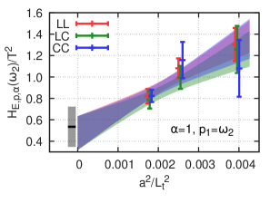
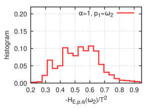
Figure 10: Left: Representative continuum extrapolation for $H_{E}(\omega_{2})/T^{2}$ using the standard subtraction (i) with $\alpha=1$ and $p_{1}=\omega_{2}$ detailed in Sec. IV.1. Right: Histogram of the Akaike-weights plotted against the continuum extrapolated results for $H_{E,p,\alpha}(\omega_{2})/T^{2}$ with $\alpha=1$ and $p_{1}=\omega_{2}$. The exact form of the integrand is in Eq. (50).

We note that on a finite lattice, the values of $H_{E,{\bf p},\bm{\alpha}}(\omega_{n})$ with different $p_{i}$ and $\alpha_{i}$ values could differ from each other, but the result for $H_{E}(\omega_{n})$ in the continuum limit estimated using $H_{E,{\bf p},\bm{\alpha}}(\omega_{n})$ with different $p_{i}$ and $\alpha_{i}$ values should be the same. One can therefore explore various choices to reduce the lattice artefacts of the continuum extrapolation.

The integrands using the general subtractions of Eq. (19) show very different behavior compared to the integrand obtained by using the standard subtraction with $p_{1}=\omega_{2}$ and $\alpha_{1}=1$ ($\alpha_{i>1}=0$). When modelling the tail of the integrands, a slightly extended version of the modelling procedure of Sec. III.2 was used due to the different noise level of the screening correlators in the different sectors. We discuss these procedures in more detail in App. C. We restrict our examination to choices which are a linear combination of the static correlator with zero and non-zero momentum and with the following relation between the coefficients defined in Eq. (19)

$$\alpha_{1} =\alpha^{2}, p_{1}>0$$ (49)

$$\alpha_{2} =1-\alpha^{2},\qquad p_{2}=0$$ (50)

In App. C, we explore a wider range of $\alpha$ values, but here we provide the results for only three choices of parameters:

1. the standard subtraction with $\alpha=1$ and $p_{1}=\omega_{2}$

2. a subtraction with $\alpha=2$ and $p_{1}=\omega_{1}$ which has the largest cancellation when Taylor-expanding in $x_{3}$ among the various terms in Eq. (50) at short distances

3. a subtraction with $\alpha=3.5$ and $p_{1}=\omega_{1}$ which has the smallest observed slope in the continuum extrapolation among the investigated values of $\alpha$ (see Tab. 2 of App. C)

We note that Eq. 50 uses the continuum notation.

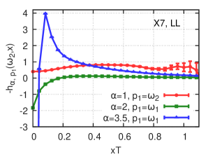
Figure 11: Comparison of the integrands obtained by applying the standard subtraction (i) (red), and more general subtractions (ii) and (iii) of the form given in Eq. (50) with $\alpha=2$, $p_{1}=\omega_{1}$ as well as $\alpha=3.5$, $p_{1}=\omega_{1}$ plotted with green and blue colors, respectively. The latter curve starts at around $-40$, which is not included on the plot.

First, we discuss the simplest of these choices, the standard subtraction (i). For this case, the modelling of the static screening correlator at $\omega_{2}$ is more challenging than it was in the first Matsubara sector, because of the worse signal-to-noise ratio above $xT\sim 0.8$. The continuum extrapolation has a moderate but significant slope (left panel of Fig. 10), and the obtained continuum limit results scatter in a wide range as the histogram in the right panel of Fig. 10 shows. This is primarily due to the uncertainty in the modelling of the static screening correlator at $p_{1}=\omega_{2}$. The obtained central value — although having a large systematic error — is in slight contradiction with the physical expectation, namely that $H_{E}(\omega_{n})<H_{E}(\omega_{r})$ if $\omega_{n}>\omega_{r}$, which is a consequence of the positivity of the transverse channel spectral function, $\sigma(\omega)$. This ordering of $H_{E}$s in various Matsubara sectors can be deduced from Eq. (12).

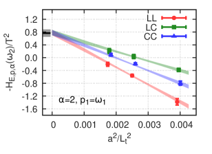
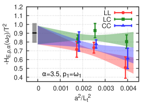
Figure 12: Representative continuum extrapolations for $H_{E}(\omega_{2})/T^{2}$ using a subtraction (ii) with $\alpha=2$ and $p_{1}=\omega_{1}$ (left panel) or with choice (iii) $\alpha=3.5$ and $p_{1}=\omega_{1}$ (right panel). The exact form of the integrand is in Eq. (50).

The subtractions (ii) and (iii) involving the static screening correlator at momentum $p=\omega_{1}$ and at vanishing momentum is advantageous over the one at $\omega_{2}$ primarily due to three reasons. First, the data has better precision because it does not involve the static screening correlator at spatial momentum $p=\omega_{2}$, therefore one can start the modelling from a later point. The details of this modified modelling prescription are discussed in App. C. Second, the plateau region is more clearly pronounced than in the case of the static screening correlator in the second Matsubara sector, which results in smaller systematic errors. Furthermore, due to the freedom of choosing $\alpha$, one can construct integrands which behave better, which are less weighted towards the noisy long-distance tail or have smaller cutoff effects.

As mentioned earlier, the integrand obtained using more general subtractions can be quite different from what we obtain using the standard subtraction. In the continuum, both $G_{\rm st}^{\rm T}(\omega_{n},x_{3})$ and $G_{\rm ns}^{\rm T}(\omega_{n},x_{3})$ are expected to have the leading singular behaviour

$$G_{\rm st}^{\rm T}(\omega_{n},x_{3}),\leavevmode\nobreak\ G_{\rm ns}^{\rm T}(\omega_{n},x_{3})\stackrel{{\scriptstyle x_{3}\to 0}}{{\sim}}\Big{(}\omega_{n}^{2}-\frac{\partial^{2}}{\partial x_{3}^{2}}\Big{)}\delta(x_{3}),$$ (51)

with the same prefactor. This explains in particular the observed smoothness of the integrand (50) for our standard choice. For subtraction (ii), the integrand would be proportional to $|x_{3}|$ at small $|x_{3}|$ in the vacuum; therefore, the thermal integrand remains finite in the continuum at $x_{3}=0$ (the difference of the static thermal and the vacuum correlator has been investigated in Cè et al. (2021b)). For all other values of $\alpha$, the integrand with $p_{1}=\omega_{1}$ has a singular behaviour around $x_{3}=0$, even though the integral has a well-defined continuum limit.

Fig. 11 shows this for the second Matsubara sector, where one can see that $-h_{\alpha=1,p_{1}=\omega_{2}}(\omega_{2},x)$, — i.e. the integrand using the standard subtraction — starts with a finite, positive value at $x=0$ and after having a modest peak it decays to zero, being quite noisy above $xT\sim 0.8$. The integrands using alternative subtractions also go to zero at large distances as earlier but the decay is faster. At $p_{1}=\omega_{1}$, the choice $\alpha=2$, results in a smooth integrand, while the one with $\alpha=3.5$, has a more singular behaviour in the vicinity of $x_{3}=0$: the latter integrand starts at $x/a=0$ with a value of about $-40$ for the finest ensemble and the LL discretisation, then it changes sign at $x/a=1$ and has a peak at $x/a=2$, after which it decays to zero. Thus, there is a large cancellation among the point at $x_{3}\lesssim 1/(4T)$. We use the trapezoid integration rule also at short distances, as we have done earlier.

The resulting continuum extrapolations using choices (ii) and (iii) are shown in Fig. 12, left and right panel, respectively. As one can observe in Fig. 12, the cutoff effects can be markedly different using different subtractions. For instance, the subtraction (ii) leads to a huge cutoff effect (left panel of Fig. 12), the results at the coarsest ensemble even have a different sign than the continuum estimate. On the contrary, the subtraction (iii) has a very flat continuum extrapolation (right panel of Fig. 12). The slopes of the continuum extrapolations are also listed in Table 2 of App. C for these subtraction types.

The continuum estimates we obtained by applying the different subtractions of the type given in Eq. (19) are the following:

(i) $$\qquad H_{E,p=\omega_{2},\alpha=1}(\omega_{2})/T^{2} =-0.54(13)_{\rm{stat}}(13)_{\rm{sys}},$$ (52)

(ii) $$\qquad H_{E,p=\omega_{1},\alpha=2}(\omega_{2})/T^{2} =-0.76(9)_{\rm{stat}}(3)_{\rm{sys}},$$ (53)

(iii) $$\qquad H_{E,p=\omega_{1},\alpha=3.5}(\omega_{2})/T^{2} =-0.90(10)_{\rm{stat}}(4)_{\rm{sys}}.$$ (54)

For further details on the modelling and the other parameters that were used to obtain these continuum estimates, we refer to App. C. In addition, in App. C, we investigate a broader set of $\alpha$ values, from which we conclude that the continuum result obtained by having a flat continuum extrapolation with $\alpha=3.5$ is a result that is in good agreement with more or less all the other results (c.f. Fig. 20 and also Fig. 21). Therefore, we choose this value,

$$H_{E}(\omega_{2})/T^{2}=-0.90(10)_{\rm{stat}}(4)_{\rm{sys}}$$ (55)

as our final continuum estimate in the second Matsubara sector.

IV.2 Direct evaluation of the difference $H_{E}(\omega_{2})-H_{E}(\omega_{1})$

Using Eq. 20, we can directly evaluate the difference of $H_{E}$s obtained in different Matsubara sectors, or more generally the difference $H_{E}(\omega_{r})-\varepsilon H_{E}(\omega_{n})$. The results obtained in this way can be compared to the results obtained by calculating $H_{E}(\omega_{r})$ and $H_{E}(\omega_{n})$ separately and thereby serve as a useful crosscheck of those results. Additionally, the difference is an interesting quantity for its own sake. For instance, the choice $\varepsilon=1$ probes an integrand, which is non-singular and is only sensitive to photons at nonzero frequencies (see Fig. 1).

We calculated the linear combination $H_{E}(\omega_{2})-\varepsilon H_{E}(\omega_{1})$ in several ways and summarized the results in Table 3 of App. C. Among the results listed in Table 3, we highlight here the ones which have the flattest continuum extrapolations. These are the subtractions that have

$$\epsilon=1,\qquad\alpha_{1}=11.25,\qquad\alpha_{2}=-11.25,$$ (56)

and

$$\epsilon=14,\qquad\alpha_{1}=0,\qquad\alpha_{2}=-13.$$ (57)

In both cases, the momentum of the subtracted non-static screening correlator is $\omega_{1}$ and the momenta of the static screening correlators are $p_{1}=\omega_{1}$ and $p_{2}=0$, for the correlators multiplied by $\alpha_{1}$ and $\alpha_{2}$, respectively. Thus, the integrand in the continuum has the exact form of

$$G_{\rm{ns}}^{\mathrm{T}}(\omega_{2},x_{3})\mathrm{e}^{-\omega_{2}x_{3}}-\varepsilon\,G_{\rm{ns}}^{\mathrm{T}}(\omega_{1},x_{3})\mathrm{e}^{-\omega_{1}x_{3}}-\alpha_{1}\,G_{\rm{st}}^{\mathrm{T}}(\omega_{1},x_{3})\mathrm{e}^{-\omega_{1}x_{3}}-\alpha_{2}\,G_{\rm{st}}^{\mathrm{T}}(0,x_{3}).$$ (58)

The results for $\varepsilon=1$ correspond to forming the difference of the integrand for $H_{E}(\omega_{2})$ that has a flattest observed continuum extrapolation (choice (iii) of the previous section, see Eq. 50) and the integrand for $H_{E}(\omega_{1})$ having a standard subtraction term (Eq. 18 with $n=1$ and $p=\omega_{1}$). Therefore, it is nice to observe that the difference obtained in the continuum limit

$$\frac{1}{T^{2}}\Big{[}H_{E}(\omega_{2})-H_{E}(\omega_{1})\Big{]}_{\bm{p}=(\omega_{1},0),\,\bm{\alpha}=(11.25,-11.25)}=-0.23(12)_{\rm{stat}}(4)_{\rm{sys}}$$ (59)

is in complete agreement with the difference formed by using the continuum estimates for $H_{E}(\omega_{2})$ and $H_{E}(\omega_{1})$, separately.

For the other set of parameters with $\epsilon=14$ for which we also observe a mild continuum extrapolation, we obtain

$$\frac{1}{T^{2}}\Big{[}H_{E}(\omega_{2})-\varepsilon H_{E}(\omega_{1})\Big{]}_{\bm{p}=(\omega_{1},0),\,\bm{\alpha}=(0,-13)}=8.44(11)_{\rm{stat}}(5)_{\rm{sys}}.$$ (60)

In order to put this into context, we calculated $H_{E}(\omega_{2})/T^{2}$ from this result by adding 14 times the continuum estimate of $H_{E}(\omega_{1})/T^{2}$ in a correlated way. We obtained $H_{E}(\omega_{2})/T^{2}=-0.94(12)_{\rm{stat}}(5)_{\rm{sys}}$, which is also in good agreement with our final estimate.

V Comparisons

In this section, we compare our findings to results from analytic approaches. We start with the integrand for $H_{E}(\omega_{1})$, which is shown in Fig. 13. The calculation of the integrand of the free continuum result requires special care at very short distances, below $xT\sim 0.1$. This is discussed in App. D. By looking at Fig. 13, we can observe that the continuum free theory result has very different characteristics compared to the lattice QCD result. Although both start with a finite value at $x=0$, the free theory result decays faster and even goes to slightly negative values above $xT\approx 1$.

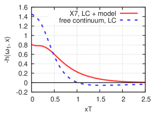
Figure 13: The integrand for determining $H_{E}(\omega_{1})$ in the free theory (dashed) and using lattice QCD data on our finest ensemble X7, completed with a model based on single-state fits for long distances using Eqs. (30),(34),(38) (solid line). Only the central values are shown.

Secondly, we summarized the comparison of the non-static screening masses determined on the lattice and the weak-coupling results in Fig. 14. We refer to App. F as well as to Ref. Brandt et al. (2014) for more detailed information about the results. As Fig. 14 shows, the lattice result for the non-static screening mass in the $n=1$ sector lies between the NLO and the EQCD result. We conclude that the weak-coupling prediction is fairly successful, at the $4\%$ level, provided at least the next-to-leading order interquark potential is used. The weak-coupling results in Fig. 14 are based on the value $\alpha_{s}=0.25$, which will be our default value of the gauge coupling in the following.

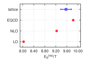
Figure 14: Ground-state non-static screening masses in the $n=1$ Matsubara sector determined on the lattice and by using weak-coupling theory at leading order (LO), with an interquark potential at next-to-leading order (NLO), and by using the potential at $T=400$ MeV of the dimensionally reduced effective theory for QCD, ’electrostatic QCD’ (EQCD).

Calculating the imaginary part of the retarded correlator at lightlike kinematics in the free massless theory with our current normalization gives $H_{E}(\omega_{n})/T^{2}=-N_{c}/6$, independently of $n$ Meyer (2018). This corresponds to a free spectral function

$$\sigma^{\rm free}(\omega)/\omega=\frac{N_{c}}{3}\pi T^{2}\,\delta(\omega),\qquad\chi_{s}^{\rm free}=\frac{N_{c}}{3}T^{2}.$$ (61)

Therefore ${H_{E}(\omega_{1})/\chi_{s}^{\rm free}=-0.500}$. This result can also be reproduced to good precision by integrating the free theory integrand shown in Fig. 13, if one uses a suitable representation (cf. appendix D).

In strongly coupled $\mathcal{N}=4$ super Yang–Mills (SYM) theory using the AdS/CFT correspondence, one finds $H_{E}(\omega_{1})/\chi_{s}^{\rm free}=-0.336$ Meyer (2018), using $(\chi_{s})^{\rm free}=N_{c}^{2}T^{2}/4$ (see Teaney (2006), appendix A). This value is in fact lower than the free-theory result. Compared in this way, the lattice result we obtained, $-0.670(6)_{\rm{stat}}(1)_{\rm{sys}}$, is largest.

Using a different normalization, e.g. dividing by the static susceptibility, $\chi_{s}$, of the relevant interacting theories we arrive at the following predictions: in the free theory, obviously the result does not change, while in $\mathcal{N}=4$ super Yang–Mills theory, we get $[H_{E}/\chi_{s}]^{\rm{(SYM)}}=-0.6715$ Meyer (2018), where $\chi_{s}=N_{c}^{2}T^{2}/8$. In Ref. Cè et al. (2022b), we determined the static susceptibility at this temperature to be

$$\chi_{s}^{\rm{(lat)}}/T^{2}=0.882(11)_{\rm{stat}}(19)_{\rm{sys}}.$$ (62)

Using this value, our lattice result is $[H_{E}/\chi_{s}]^{\rm{(lat)}}\simeq-0.76$. Thus, now normalizing by the interacting $\chi_{s}$, the lattice result is still the largest in magnitude. These results are illustrated in Fig. 15.

In the second Matsubara sector, we have $-1.115$ for $H_{E}(\omega_{2})/T^{2}$ in strongly coupled $\mathcal{N}=4$ SYM Meyer (2018), thus the difference $(H_{E}(\omega_{2})-H_{E}(\omega_{1}))/\chi_{s}$ is $-0.444$, a value larger than our lattice result by 1.7 standard deviations. Since $H_{E}(\omega_{n})$ is constant in the free theory, the difference vanishes there. Thus the ratio $(H_{E}(\omega_{2})-H_{E}(\omega_{1}))/H_{E}(\omega_{1})$ provides good sensitivity to the shape of $\sigma(\omega)$, being 0.66 in the strongly-coupled SYM case and parametrically small in the case of a spectral function very peaked around $\omega=0$. The lattice result, $(H_{E}(\omega_{2})-H_{E}(\omega_{1}))/H_{E}(\omega_{1})=0.34\pm 0.19$, lies between these two extremes.

V.1 Computing $H_{E}(\omega_{n})$ dispersively using the complete leading-oder $\sigma(\omega)$

Using the complete leading-order result of Arnold, Moore and Yaffe (AMY) for $\sigma(\omega)$ Arnold et al. (2001b, a), the difference $[H_{E}(\omega_{2})-H_{E}(\omega_{1})]$ can be evaluated straightforwardly, whereas the quantity $H_{E}$ in individual Matsubara sectors can only be estimated after handling the singular behavior of $\sigma_{\rm{AMY}}(\omega)$ at small frequencies. Indeed, by integrating the spectral function of Ref. Arnold et al. (2001b, a) (with $\alpha_{s}=0.25$) multiplied by the kernel $\omega_{n}^{2}/(\pi\omega(\omega^{2}+\omega_{1}^{2}))$ in the range $0.2<\omega/T<50$ where the provided parametrisation is a good approximation, we obtain

$$\Big{[}H_{E}(\omega_{1})/T^{2}\Big{]}_{\rm{LO},\,0.2<\omega/T<50}\approx-0.75,$$ (63)

which is already larger in absolute value than the result obtained on the lattice. On the other hand, the prediction for $H_{E}(\omega_{2})-H_{E}(\omega_{1})$ using the AMY spectral function is much less sensitive to the small-$\omega$ behaviour. We obtain, again with $\alpha_{s}=0.25$,

$$\Big{[}H_{E}(\omega_{2})/T^{2}-H_{E}(\omega_{1})/T^{2}\Big{]}_{\rm{LO},\,0.2<\omega/T<50}\approx-0.25.$$ (64)

The comparison can be seen in Fig. 15, right panel. The leading-order prediction for this difference is well compatible with our lattice QCD result. We also note that extending the integral to $\omega=\infty$ assuming $\sigma(\omega)\propto\sqrt{\omega}$ Arnold et al. (2001a) changes the value of Eq. (64) to $-0.28$.

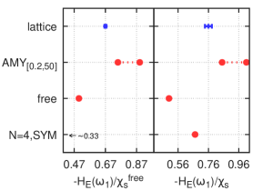
Figure 15: Left: Comparison of results for $H_{E}(\omega_{1})$ obtained on the lattice, in leading order of the weak-coupling expansion (with $\alpha_{s}=0.25$ ($\alpha_{s}=0.31$) for the left (right) point), in the free theory and in strongly coupled $\mathcal{N}=4$ SYM, normalized by the static susceptibility of the corresponding non-interacting theory (left inset), or by the interacting static susceptibility (right inset). We interpret the two normalizations as being identical for the “free” data points, while to normalize the NLO results we used alternatively 1 and the lattice result 0.88 for $\chi_{s}/T^{2}$. Right: Comparison for $H_{E}(\omega_{2})-H_{E}(\omega_{1})$ with the same choices of normalization.

In order to exploit our precise lattice result for $H_{E}(\omega_{1})$, we need to inspect more precisely the region of validity of the weak-coupling spectral function. The leading-order calculation Arnold et al. (2001b, a) assumes the photon wavelength to be short compared to the mean free path for large-angle scattering. At the smallest frequencies at which the calculation is still valid, $\sigma(\omega)\propto 1/\sqrt{\omega}$. Since we expect $\sigma(\omega)/(2\chi_{s}\omega)$ to tend to a finite value at $\omega\to 0$, namely to the diffusion coefficient $D$ (see Eq. (14)), it is clear that a qualitative change in the functional form must take place below the frequency at which the AMY calculation breaks down. In addition, the next-to-leading order correction Ghiglieri et al. (2013), suppressed only by one power of the strong coupling $g$, turns out to be quite modest (about $\pm 10\%$) for $\omega\gtrsim 2\pi T$, but becomes larger (about $\pm 30\%$) at $\omega\lesssim\pi T$.

Thus a qualitative modification of the AMY spectral function at small frequencies is necessary for a sensible dispersive evaluation of $H_{E}(\omega_{1})$. In the following, we assume that $\sigma(\omega)$ is given by the leading-order expression Arnold et al. (2001a) for $\omega>\omega_{\rm m}$, introduce a Lorentzian ansatz for $\omega<\omega_{\rm m}$,

$$\frac{\sigma(\omega)}{2\chi_{s}\omega}=\frac{A}{\omega^{2}+\eta^{2}},$$ (65)

and require continuity and differentiability at $\omega=\omega_{\rm m}$. Depending on $\omega_{\rm m}$, different values of $H_{E}(\omega_{1})$, and of $D=A/\eta^{2}$, are obtained. At the high-frequency end, we extend $\sigma(\omega)$ beyond $\omega=50T$ assuming $\sigma(\omega)\propto\sqrt{\omega}$, though this high-energy region only contributes about $-0.01$ to $H_{E}(\omega_{1})/T^{2}$.

The leading-order weak-coupling result for $D$ is known from Ref. Arnold et al. (2003): with $m_{D}/T=2.05$, which results from setting $\alpha_{s}=0.25$ in the leading order expression of the Debye mass, we read off $T\cdot D=2.3$ from Fig. 1 of Arnold et al. (2003). It turns out that this value of the diffusion coefficient can be reproduced by choosing the matching point at $\omega_{\rm m}=0.50T$, using $\alpha_{s}=0.25$ as well in the weak-coupling spectral function $\sigma(\omega)$ Arnold et al. (2001a). In that case, however, the dispersive integral yields $H_{E}(\omega_{1})/T^{2}=-0.99$, in stark disagreement with our lattice result (41). Thus this particular weak-coupling scenario is ruled out at $T=250\,$MeV by our lattice calculation.

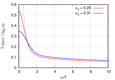
Figure 16: Two weak-coupling based spectral functions reproducing the value (41) for $H_{E}(\omega_{1})$. Beyond a value $\omega=\omega_{\rm m}$ marked by a short vertical line, the curves correspond to the complete leading-order result in the parametrization provided by Arnold et al. (2001a), for two values of $\alpha_{s}$. For $\omega<\omega_{\rm m}$, the curves correspond to the Lorentzian (65) with parameters given in Eqs. (66–67), respectively. In the $\alpha_{s}=0.25$ case, the dashed curve shows how the parametrization of Arnold et al. (2001a) extends towards smaller frequencies. The intercept at $\omega=0$ yields the isospin diffusion coefficient, $T\cdot D$.

Instead of assuming the weak-coupling result for the diffusion coefficient, we can attempt to estimate it by continuing the leading-order expression Arnold et al. (2001a) of $\sigma(\omega)$ toward the soft-photon limit via the Lorentzian Eq. (65) so as to reproduce our lattice result for $H_{E}(\omega_{1})$. With $\alpha_{s}=0.25$, this condition yields

$$\alpha_{s}=0.25:\quad\omega_{\rm m}=1.08\,T,\qquad A=0.42\,T,\qquad\eta=0.88\,T,\qquad T\cdot D=0.54.$$ (66)

Increasing the targeted $|H_{E}(\omega_{1})|/T^{2}$ by one standard deviation (0.006) only results in a modest change in the estimated diffusion coefficient to $T\cdot D=0.56$. Thus the estimate of the diffusion coefficient obtained in this way is much lower than the weak-coupling result Arnold et al. (2003), but still more than three times larger than the AdS/CFT value of $D=(2\pi T)^{-1}$. Repeating the procedure above with a larger value of the coupling, we obtain

$$\alpha_{s}=0.31:\quad\omega_{\rm m}=1.50\,T,\qquad A=0.78\,T,\qquad\eta=1.50\,T,\qquad T\cdot D=0.35.$$ (67)

In summary, under the assumptions made on the spectral function, we obtain a range of diffusion coefficients given by Eqs. (66–67). The corresponding spectral functions are illustrated in Fig. 16.

It is worth recalling that in the non-interacting theory, the spectral function has the form $\omega\delta(\omega)$ (see Eq. (61)). In the limit of vanishing coupling, one thus expects the Lorentzian to turn into a delta function ($\eta\to 0$ at fixed $A/\eta$), and the spectral function to vanish roughly proportionally to $\alpha_{s}$ for $\omega\gg\eta$. We define the area under the peak around $\omega=0$ as follows,

$$S_{0}\equiv\int_{-\Omega}^{\Omega}\frac{d\omega}{\pi}\;\frac{\sigma(\omega)}{2\chi_{s}\omega},$$ (68)

where $\Omega\gg\eta$ is a UV-cutoff. On the one hand, we get with our Lorentzian ansatz $S_{0}={A}/{\eta}$. In the free theory, one obtains $S_{0}=1/2$. Thus it is remarkable that the ratios $A/\eta$ in Eqs. (66–67) are close to $1/2$: the obtained values of the parameters $(A,\eta)$ are plausible in this respect, since our analysis is based on an ansatz for the spectral function valid at weak coupling and $S_{0}$ has a weak-coupling expansion of which $S_{0}=1/2$ is the leading term.

VI Conclusions and outlook

The thermal photon emissivity of the quark-gluon plasma is determined to all orders in the strong coupling by the transverse channel spectral function of electromagnetic current-current correlators evaluated at lightlike kinematics. This real-time observable is not accessible directly on a Euclidean lattice. In this work, we demonstrated that it is nonetheless possible to directly evaluate an observable in lattice QCD that is related to the aforementioned spectral function via a dispersion relation. Indeed, the computed observable — a Euclidean screening correlator at imaginary spatial momentum — has an integral representation in terms of a product of the spectral function multiplied by a Lorentzian kernel (see Eq. 13). However, the naive lattice estimator of this observable is afflicted by a large cutoff effect arising from the breaking of Lorentz invariance on the lattice. We successfully addressed this technical difficulty by subtracting screening correlators at different momenta, whose contribution vanishes in the continuum. We investigated various subtractions which lead to different scaling behaviors towards the continuum limit.

By analyzing the long-distance behavior of the screening correlators, we also determined the screening masses (see Eqs. (43,45,46)), which we used to model the position-space correlators at long distances and improve the precision of the imaginary-momentum correlators. In order to probe the virtuality dependence of the latter around the $Q^{2}=0$ point, we constructed a suitable lattice representation of its $Q^{2}$-derivative and evaluated it in the first Matsubara sector. We used two-flavors of O($a$)-improved Wilson fermions at a temperature of about 250 MeV with an in vacuo pion mass of 270 MeV and performed continuum extrapolations of all our observables.

Our final continuum result for $H_{E}(\omega_{1})/T^{2}$, see Eq. (41), has a precision of around 1%, suitable for a comparison with other approaches. We confronted our results to estimates using the free theory, strongly-coupled $\mathcal{N}=4$ SYM and the full leading-order result of Arnold, Moore and Yaffe (AMY) Arnold et al. (2001b, a). We found that our result for $|H_{E}(\omega_{1})|$ is smaller than the prediction obtained by using the spectral function of Ref. Arnold et al. (2001b, a), although our result for $H_{E}(\omega_{2})-H_{E}(\omega_{1})$, given in Eq. (59), is comparable. This is illustrated in Fig. 15. Since the integration kernel is much more sensitive to the low-frequency behavior of the spectral function in the case of $H_{E}(\omega_{n})$ than in the case of the difference (c.f. Fig. 1), our result suggests that the weak-coupling result for the spectral function is overestimated in this low-frequency region. Assuming the AMY spectral function to hold above a certain frequency $\omega_{\rm m}$, and using a Lorentzian transport peak below that frequency that matches on smoothly at $\omega_{\rm m}$, we arrive at estimates of the isospin diffusion coefficient $T\cdot D$ in the range 0.35 to 0.54 (see Eqs. 66–67) by requiring that our lattice result for $H_{E}(\omega_{1})$ be reproduced. This range of values for $T\cdot D$ is in line with previous lattice estimates based on dispersion relations at fixed spatial momentum Brandt et al. (2013); Amato et al. (2013); Aarts et al. (2015); Brandt et al. (2016); Ghiglieri et al. (2016); Ding et al. (2016); Astrakhantsev et al. (2020), though the central values of most calculations with dynamical quarks lie below the value of 0.3 at temperatures around 250 MeV Aarts and Nikolaev (2021).

It is also interesting to compare our results with our two previous studies of the photon emissivity that employed the same gauge ensembles as the present calculation but were based on the dispersion relation at fixed spatial momentum Cè et al. (2021b, 2022b). Addressing the inverse problem with physically motivated ansätze for the spectral functions, we concluded Cè et al. (2022b) (particularly for $\omega\geq\pi T$) that the lattice results were consistent with the weak-coupling prediction, but could also accomodate a rate 2.5 times larger. In other words, most of the solutions for the spectral function describing the lattice data yielded a photon rate at least as large as the weak-coupling prediction. Given that the weak-coupling spectral function Arnold et al. (2001a) results in a larger value for $|H_{E}(\omega_{1})|$ than our lattice result, it seems most likely that this excess is due to an overestimated soft-photon emissivity in the weak-coupling calculation.

We have seen that computing $H_{E}(\omega_{2})$ by standard lattice methods is already a lot more challenging than for $H_{E}(\omega_{1})$ due to the large statistical errors on the position-space integrand. Thus it would be interesting to investigate noise-reduction methods similar to those used in calculations of the hadronic vacuum polarization. Improving on our determination of $H_{E}(\omega_{2})-H_{E}(\omega_{1})$ would go a long way to ascertain that the emission rate of hard photons $(\omega\gtrsim\pi T)$ follows the weak-coupling prediction at the temperatures reached in heavy-ion collisions. This appears to be an achievable goal in the near future.

A second difficulty that occurred is the increase in discretization errors for increasing $\omega_{n}$. Perhaps some improvements in the discretization are still possible here, but it is clear that very fine lattices are necessary in order to determine $H_{E}(\omega_{3})$ and beyond. While the moments $H_{E}(\omega_{n})$ provide valuable non-perturbative constraints on the spectral function, a numerically ill-posed inverse problem resurfaces if one has the ambition of determining $\sigma(\omega)$ itself from a (necessarily) finite collection of its moments. Instead, our immediate plan is to compute the first moment of $\sigma(\omega)$ across the phase crossover with physical quark masses in order to test the models of $\sigma(\omega)$ used in hydrodynamics-based calculations of photon spectra in heavy-ion collisions.

VII Acknowledgements

This work was supported by the European Research Council (ERC) under the European Union’s Horizon 2020 research and innovation program through Grant Agreement No. 771971-SIMDAMA, as well as by the Deutsche Forschungsgemeinschaft (DFG, German Research Foundation) through the Cluster of Excellence “Precision Physics, Fundamental Interactions and Structure of Matter” (PRISMA+ EXC 2118/1) funded by the DFG within the German Excellence strategy (Project ID 39083149). The research of M.C. is funded through the MUR program for young researchers “Rita Levi Montalcini”. The generation of gauge configurations as well as the computation of correlators was performed on the Clover and Himster2 platforms at Helmholtz-Institut Mainz and on Mogon II at Johannes Gutenberg University Mainz. We have also benefited from computing resources at Forschungszentrum Jülich allocated under NIC project HMZ21. For generating the configurations and performing measurements, we used the openQCD Luscher and Schaefer (2013) as well as the QDP++ packages Edwards and Joo (2005), respectively.

Appendix A Elimination of outliers

In this Appendix, we describe our procedure to deal with certain measurements that deviate by several standard deviations from the mean value calculated using the data. We identify these exceptional measurements as outliers, see the left panel of Fig. 17 and we found, they occur more frequently at large Euclidean separations. These outliers increased the statistical error and also modified the mean to some extent, see Fig. 17, right panel. We eliminated them by using robust statistics P. J. Huber (2009).

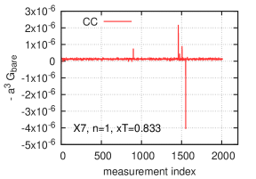
Figure 17: Left: Measurement history of the non-static screening correlator at $xT=0.833$. The outliers are shown up as spikes in the data. Right: Truncation stability for the non-static screening correlator. The data points corresponding to the trimmed data have been shifted slightly to the right to improve visibility.

In our procedure, we first prepared a distribution of results at each Euclidean distance, then removed the data points belonging to the lower and upper $\gamma$% of that distribution. Varying $\gamma$ in the interval 0.5–4, we made cuts and found that the error estimation as well as the calculation of the mean is more stable this way. When we detected only less than 10 datapoints being outside five times the interquantile range from the mean, we applied only a trimming with $\gamma=0.5$. For other distances we applied $\gamma=1$ in our final analysis.

We show an example in the case of the conserved-conserved correlator on our finest ensemble, X7, in the right panel of Fig. 17. At short distances of the correlator, this approach did not influence the results, because outliers occured there only very rarely. At intermediate distances, i.e. around $xT\sim 0.7$–$1.3$, the effect of this method was again not significant. At large distances, however, the errors reduced by a factor of around 2–6 when omitting the tails of the distributions. Although one has to be careful when discarding certain measurements, we believe that our procedure removing outliers sometimes more than 10 standard deviations off from the mean at large distances should not influence the validity of the extracted physical results.

Appendix B Alternative subtractions for determining $H_{E}(\omega_{1})$

In this appendix, we discuss the determination of $H_{E}(\omega_{1})$ using a more general class of subtractions to tame the short-distance cutoff effects.

Besides the standard subtraction in the first Matsubara sector (Eq. (18) with $p=\omega_{1}$), we calculate $H_{E}(\omega_{1})/T^{2}$ by integrating the integrand formed by subtracting the completely static screening correlator ($n=0$) from the non-static screening correlator at the $n=1$ Matsubara sector. This latter is denoted by $H_{E,p=0}(\omega_{1})/T^{2}$, while the results obtained using the standard subtraction are denoted by $H_{E,p=\omega_{1}}(\omega_{1})/T^{2}$ in this appendix. We note, that in the main text, we left the lower subscript $p$, because we used the standard subtraction when discussing $H_{E}$ in the first Matsubara sector in Secs. III.1,III.2 and III.3.

The integrand obtained by subtracting the completely static screening correlator ($p=0$) is quite different than it was in the case of subtracting the static correlator at $p=\omega_{1}$. At larges distances it goes to zero as earlier, but with different sign. It receives a huge contribution from very short distances, $xT\sim 0$, since it starts at $x/a=0$ with a large value, then it changes sign at $x/a=1$.

We emphasize here that on a finite lattice, the values of $H_{E,p}(\omega_{n})$ with different $p$ differ from each other, but the result for $H_{E}(\omega_{n})$ in the continuum limit estimated using $H_{E,p}(\omega_{n})$ with different $p$ values should agree. In Fig. 18, we compare the continuum extrapolations using $p=\omega_{1}$ — which was our standard choice in previous sections — to using $p=0$, i.e. when we subtract the completely static, zero-momentum screening correlator when forming the integrand in Eq. (18).

As one can observe on Fig. 18, the continuum extrapolation is much steeper in the case of $H_{E,p}(\omega_{1})$ with $p=0$, although the linear scaling in $a^{2}$ persists. Repeating a similar continuum procedure for $H_{E,p}(\omega_{1})$ with $p=0$ as was discussed for $H_{E,p}(\omega_{1})$ with $p=\omega_{1}$ in Sec. III.3, we found quantitatively similar fit qualities. Using $p=0$ in Eq. (18), the estimate for $H_{E}(\omega_{1})/T^{2}$ in the continuum is

$$\lim_{a^{2}\to 0}H_{E,p=0}(\omega_{1};a)/T^{2}=-0.653(6)_{\rm{stat}}(2)_{\rm{sys}},$$ (69)

which is 1.9 standard deviations smaller than the continuum results obtained using the data with $p=\omega_{1}$, c.f. Eq. (41).

This discrepancy can be either attributed to the breakdown of the trapezoid integration around $xT\sim 0$ or to the steeper continuum extrapolation and the presence of higher order lattice artifacts which we could not resolve at the current precision. On the other hand, this agreement to 1.9 $\sigma$ is quite remarkable in view of the different magnitude of the $a^{2}$ coefficients in the continuum extrapolation, which are more than an order of magnitude larger in absolute value when using $p=0$ instead of $p=\omega_{1}$.

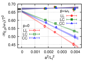
Figure 18: Comparison of representative continuum extrapolations for $H_{E}(\omega_{1})/T^{2}$ using $H_{E,p=\omega_{1}}(\omega_{1})/T^{2}$ or $H_{E,p=0}(\omega_{1})/T^{2}$ with filled and open symbols, respectively.

Appendix C More details on the alternative subtractions for determining $H_{E}(\omega_{2})$

In this appendix, we discuss more details about the more general alternative subtractions of which we presented a few results in Sec. IV.1.

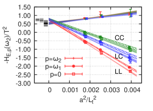
Figure 19: Comparison of representative continuum extrapolations for $H_{E}(\omega_{2})/T^{2}$ using $\alpha=1$ and $p_{1}=\omega_{2}$, $p_{1}=\omega_{1}$ or $p_{1}=0$. Different colors correspond to different discretizations (local-local (LL): red, local-conserved (LC): blue, conserved-conserved (CC): green). Note the gigantic lattice artifacts when subtracting the static screening correlator with $p_{1}=\omega_{1}$ or $p_{1}=0$.

When subtracting the static screening correlator at $p=\omega_{2}$, we applied the same procedure as was discussed for $H_{E}(\omega_{1})/T^{2}$ in Sec. III.2. Since the data in the second Matsubara sector is noisier, we had to start the modelling from an earlier distance, therefore we applied $x_{\rm{w,ns}}T=0.6,0.7$.

When subtracting the static screening correlator at $p=\omega_{1}$ or at $p=0$, we slightly modified the procedure of modelling the integrand. We divided the integration interval into three parts. At short distances, both the non-static and static screening correlators have good signal-to-noise ratios, therefore we applied no modelling there. At the intermediate interval, the non-static screening correlator is already modelled but the static screening correlator is not. In this interval, we calculate the integral using the trapezoidal rule applied for the integrand formed by evaluating the single-state fit used for modelling the non-static screening correlator at the lattice points and subtracting the lattice data for the static screening correlators. Finally, in the interval for large distances, we modelled the static screening correlators as well and applied Eqs. (38) and (39). We start applying modelling by single-state fits using the smooth step function of Eq. (35) from $x_{w,\rm{ns}}T=0.6,0.7$ in the case of the non-static screening correlator in the second Matsubara sector and from $x_{w,\rm{st}}T=1.0,1.1,1.2,1.3$ in the case of the static screening correlator at $p=\omega_{1}$ or at $p=0$.

After evaluating the integrals, we performed the continuum extrapolations in a similar manner as was discussed in Sec. III.3. The continuum limit fit form is

$$f(a/\beta,A_{0},{\bf A}^{\delta})=A_{0}+A_{1}^{\delta}\times\,(a/L_{t})^{2},$$ (70)

where $A_{0}$ is the estimate of the continuum limit from a particular fit, and the $A_{1}^{\delta}$ parameters characterize the approach to the continuum of the $H_{E}$ values calculated using the different discretized correlators. $\delta$ stands for LL, LC or CC.

First, we present results that were obtained using the simple alternative subtraction of Eq. (18) but with $p=\omega_{1}$ or $p=0$. Although the lattice artefacts are huge in the case of $H_{E,p=0}(\omega_{2})/T^{2}$ and $H_{E,p=\omega_{1}}(\omega_{2})/T^{2}$, the fit qualities of the continuum extrapolations using Eq. (70), i.e. a linear fit ansätze in $a^{2}$ turned out to be acceptable. For instance, only around $\sim 2\%$ of all the $p$-values is smaller than 0.05. The estimates in the continuum using these subtractions are:

$$\lim_{a^{2}\to 0}H_{E,p=0}(\omega_{2};a)/T^{2} =-0.74(8)_{\rm{stat}}(5)_{\rm{sys}},$$ (71)

$$\lim_{a^{2}\to 0}H_{E,p=\omega_{1}}(\omega_{2};a)/T^{2} =-0.71(12)_{\rm{stat}}(4)_{\rm{sys}}.$$ (72)

Depending on the actual modelling interval, the results could be slightly different, but stay consistent within errors. These subtractions bring only a modest improvement: the modelling is more precise, but the slope of the continuum extrapolations are huge (see Fig. 19).

Applying the more general subtractions of Eq. (19) and Eq. (20), we determined $H_{E}(\omega_{2})/T^{2}$ using a broad set of parameters. We discussed a subset of these results in Secs. IV.1 and  IV.2. The results employing a subtraction with vanishing $\varepsilon$ are labelled as fitI and are listed in Table 2. For those subtractions we used a single parameter, $\alpha$, with which the integrand can be described as in Eq. (50). Besides the parameters that characterize the start of the modelling of the non-static as well as the static screening correlators using single state fits ($Tx_{w,{\rm{ns}}}$ and $Tx_{w,{\rm{st}}}$, respectively), we also list the fit parameters ($A_{1}^{\rm{LL}},A_{1}^{\rm{LC}},A_{1}^{\rm{CC}}$) that characterize the slopes of the continuum extrapolations in Table 2. Using these values, one can read off that the subtraction of the form of Eq. 50 gives the flattest continuum extrapolation with the choice of $\alpha=3.5$. With this value, the slope parameters of the continuum extrapolation are consistent with zero for the local-conserved and conserved-conserved discretizations. We summarize the various results for $H_{E}(\omega_{2})/T^{2}$ using these type of alternative subtractions in Fig. 20.

Turning to the subtractions that involve the non-static correlators at $\omega_{2}$ and $\omega_{1}$ as well, we applied a similar ’two-interval’ modelling procedure as we discussed above, but used a larger $Tx_{w,{\rm{st}}}$ value for the non-static screening correlator in the first Matsubara sector as well. The results employing this type of subtraction with non-vanishing $\varepsilon$ are labelled as fitII and are listed in Table 3. In Table 3, all results correspond to the choice $(Tx_{w,{\rm{ns}}},Tx_{w,{\rm{st}}})=(0.7,1.1)$; as we did earlier (see e.g. in Table 2), we performed a scan varying these parameters, but found only small changes.

It is useful to recall that the subtractions using Eq. (20) (see also Eq. (58)) enable a direct calculation of the difference of $H_{E}$s in different Matsubara sectors. We discussed two of these type of results in Sec. IV.2. In Table 3, more of these types of results are reviewed. Since the continuum extrapolated quantity is $[H_{E}(\omega_{2})-\varepsilon H_{E}(\omega_{1})]_{\bm{p},\bm{\alpha}}$ in this case, we also included a column denoted by $A_{0}$, that explicitly contains this estimate. By adding $\varepsilon\cdot H_{E}(\omega_{1})/T^{2}$ to this value, one can obtain an estimate for $H_{E}(\omega_{2})/T^{2}$. We did this in a correlated way, and then estimated the statistical error on $H_{E}(\omega_{2})/T^{2}$ and added the systematic errors in quadrature. The results of Table 3 are summarized for better overview in Fig. 21.

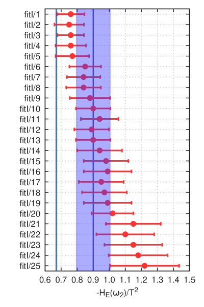
Figure 20: Comparison of continuum extrapolations for $H_{E}(\omega_{2})/T^{2}$ using various subtractions. The parameters of the various fits are listed in Table 2. The final estimate for $H_{E}(\omega_{2})/T^{2}$ is shown with a blue vertical band. The final estimate for $H_{E}(\omega_{1})/T^{2}$ is also shown for comparison with a green vertical band.

fit	$\alpha$	$Tx_{\rm{w,ns}}$	$Tx_{\rm{w,st}}$	$-H_{E}(\omega_{2})/T^{2}$	$A_{1}^{\rm{LL}}$	$A_{1}^{\rm{LC}}$	$A_{1}^{\rm{CC}}$
fitI/1	2.0	0.6	1.1	0.76(8)(3)	540(31)(11)	294(37)(15)	390(30)(12)
fitI/2	2.0	0.7	0.9	0.75(9)(2)	542(36)(10)	295(30)(16)	388(30)(11)
fitI/3	2.0	0.7	1.0	0.76(8)(2)	540(30)(11)	295(36)(15)	390(30)(12)
fitI/4	2.0	0.7	1.1	0.76(9)(3)	539(38)(11)	292(39)(16)	387(40)(12)
fitI/5	2.0	0.7	1.3	0.77(10)(3)	544(44)(12)	297(39)(20)	396(42)(16)
fitI/6	3.0	0.6	1.1	0.85(9)(4)	266(48)(14)	131(45)(21)	193(46)(16)
fitI/7	3.0	0.7	1.0	0.84(10)(3)	268(37)(14)	135(49)(18)	193(36)(16)
fitI/8	3.0	0.7	1.1	0.84(10)(4)	265(43)(14)	128(48)(22)	191(40)(16)
fitI/9	3.0	0.7	1.3	0.88(12)(4)	279(56)(16)	144(53)(24)	208(47)(23)
fitI/10	3.5	0.6	1.1	0.90(10)(4)	90(43)(16)	25(51)(27)	65(56)(18)
fitI/11	3.5	0.6	1.3	0.94(11)(4)	101(55)(18)	36(55)(29)	79(56)(19)
fitI/12	3.5	0.7	1.0	0.89(10)(4)	88(48)(16)	25(51)(25)	62(44)(18)
fitI/13	3.5	0.7	1.1	0.90(10)(4)	89(49)(17)	24(51)(27)	63(52)(18)
fitI/14	3.5	0.7	1.3	0.94(13)(5)	101(57)(19)	36(51)(31)	81(63)(24)
fitI/15	4.0	0.6	1.1	0.98(13)(5)	-118(53)(21)	-99(56)(36)	-82(57)(22)
fitI/16	4.0	0.6	1.2	0.99(14)(5)	-114(60)(23)	-98(58)(37)	-79(60)(23)
fitI/17	4.0	0.7	1.0	0.95(13)(5)	-118(57)(18)	-101(48)(32)	-87(51)(20)
fitI/18	4.0	0.7	1.1	0.97(13)(5)	-119(60)(21)	-100(60)(37)	-83(60)(22)
fitI/19	4.0	0.7	1.2	0.99(14)(5)	-113(57)(23)	-98(54)(38)	-80(55)(23)
fitI/20	4.0	0.7	1.3	1.02(12)(6)	-97(58)(23)	-75(60)(26)	-60(58)(26)
fitI/21	5.0	0.6	1.1	1.15(16)(6)	-601(68)(30)	-388(76)(43)	-430(72)(33)
fitI/22	5.0	0.7	1.0	1.10(17)(6)	-613(64)(28)	-394(82)(46)	-443(65)(27)
fitI/23	5.0	0.7	1.1	1.15(17)(6)	-601(71)(30)	-388(71)(43)	-431(73)(33)
fitI/24	5.0	0.7	1.2	1.18(17)(7)	-589(85)(31)	-379(75)(41)	-421(78)(35)
fitI/25	5.0	0.7	1.3	1.22(20)(8)	-574(77)(30)	-360(75)(46)	-403(80)(35)

Table 2: Results for $H_{E}(\omega_{2})/T^{2}$ using alternative subtractions of the form given in Eq. (19). The values of the momentum in the subtraction given in Eq. (19) are $p_{1}=\omega_{1}$ and $p_{2}=0$. $\alpha$ is a single parameter in Eq. (19), that fixes $\alpha_{1}$ and $\alpha_{2}$: $\alpha_{1}=\alpha^{2}$, $\alpha_{2}=1-\alpha^{2}$.

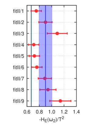
Figure 21: Comparison of continuum extrapolations for $H_{E}(\omega_{2})/T^{2}$ using various subtractions involving also the non-static correlator at $\omega_{1}$. The parameters of the various fits are listed in Table 3. The final estimate for $H_{E}(\omega_{2})/T^{2}$ is shown with a blue vertical band. The final estimate for $H_{E}(\omega_{1})/T^{2}$ is also shown for comparison with a green vertical band.

fit	$\varepsilon$	$\alpha_{1}$	$\alpha_{2}$	$-H_{E}(\omega_{2})/T^{2}$	$A_{0}$	$A_{1}^{\rm{LL}}$	$A_{1}^{\rm{LC}}$	$A_{1}^{\rm{CC}}$
fitII/1	1	3	-3	0.75(8)(3)	-0.089(88)(25)	544(36)(11)	298(34)(15)	392(32)(12)
fitII/2	1	11.25	-11.25	0.90(10)(4)	-0.23(12)(4)	93(51)(17)	31(51)(21)	65(47)(18)
fitII/3	1	24	-24	1.09(15)(6)	-0.43(17)(6)	-609(68)(28)	-391(72)(45)	-442(66)(26)
fitII/4	1	0	0	0.71(8)(3)	-0.036(89)(25)	707(39)(11)	394(36)(15)	511(39)(11)
fitII/5	2	0	-1	0.72(8)(3)	0.62(9)(3)	656(35)(11)	365(32)(16)	474(35)(11)
fitII/6	4	0	-3	0.76(8)(3)	1.92(8)(3)	554(37)(12)	306(37)(17)	398(40)(12)
fitII/7	12.25	0	-11.25	0.89(10)(4)	7.30(10)(4)	136(42)(17)	64(44)(25)	86(46)(18)
fitII/8	14	0	-13	0.94(12)(5)	8.44(11)(5)	49(40)(18)	13(46)(26)	20(49)(20)
fitII/9	25	0	-24	1.14(16)(6)	15.62(15)(6)	-502(53)(26)	-308(63)(33)	-396(67)(26)

Table 3: Results for $H_{E}(\omega_{2})/T^{2}$ using alternative subtractions with $\varepsilon\neq 0$. The formula for the integrand is given in Eq. (19). The continuum limit fit ansatz parameters (see Eq. 70) are also listed in the table.

Appendix D Free theory computation of the integrand for $H_{E}(\omega_{1})$

In this appendix, we provide the expressions for the correlators of interest in the case of non-interacting quarks. Let $G^{(-1/2)}_{m}(x_{3})=e^{-m|x_{3}|}/(2m)$ be the one-dimensional scalar propagator. Consider the function

$$H(\vec{q},\vec{s},x_{3},\tilde{x}_{3}) =\int\frac{d^{d-1}p}{(2\pi)^{d-1}}\,e^{i\vec{p}\cdot\vec{s}}\,G^{(-1/2)}_{\sqrt{\vec{p}^{2}+m^{2}}}(x_{3})G^{(-1/2)}_{\sqrt{(\vec{p}+\vec{q})^{2}+m^{2}}}(\tilde{x}_{3})$$ (73)

$$=\int\frac{d^{d-1}p}{(2\pi)^{d-1}}\;e^{i\vec{p}\cdot\vec{s}}\frac{1}{4\pi}\int_{0}^{\infty}\frac{dt}{\sqrt{t}}\,e^{-t(\vec{p}^{\,\,2}+m^{2})-x_{3}^{2}/(4t)}\int_{0}^{\infty}\frac{du}{\sqrt{u}}\,e^{-u((\vec{p}+\vec{q})^{2}+m^{2})-\tilde{x}_{3}^{2}/(4u)}$$

$$=\frac{1}{32\pi^{5/2}}\int_{0}^{\infty}\frac{dt}{\sqrt{t}}\int_{0}^{\infty}\frac{du}{\sqrt{u}}\,\frac{1}{(t+u)^{3/2}}$$ (74)

$$\quad\,\exp[-(x_{3}^{2}/t+\tilde{x}_{3}^{2}/u)/4-m^{2}(t+u)-u\vec{q}^{\,\,2}+(u\vec{q}-i\vec{s}/2)^{2}/(t+u)\Big{]}.$$ (75)

Now we can write

$$G^{\rm T}_{\rm{ns}}(\omega_{n},x_{3}) \equiv-\int\mathrm{d}x_{1}\mathrm{d}x_{2}\int_{0}^{\beta}\mathrm{d}x_{0}\,\mathrm{e}^{i\omega_{n}x_{0}}\langle J_{1}(x)J_{1}(0)\rangle$$ (76)

$$=\frac{N_{c}}{\beta}\sum_{p_{0}}^{F}\int\frac{d^{2}p_{\perp}}{(2\pi)^{2}}\frac{e^{-(E_{\vec{p}}+E_{\vec{p}+\omega_{n}\vec{e}_{0}})|x_{3}|}}{E_{\vec{p}}\,E_{\vec{p}+\omega_{n}\vec{e}_{0}}}\Big{(}E_{\vec{p}}E_{\vec{p}+\omega_{n}\vec{e}_{0}}+p_{0}(p_{0}+\omega_{n})+m^{2}\Big{)}$$ (77)

$$=4N_{c}\sum_{n_{s}\in\mathbb{Z}}(-1)^{n_{s}}\Big{(}\frac{\partial^{2}}{\partial x_{3}\partial\tilde{x}_{3}}-\frac{\partial^{2}}{\partial s_{0}^{2}}-i\omega_{n}\frac{\partial}{\partial s_{0}}+m^{2}\Big{)}H(\vec{q},\vec{s},x_{3},\tilde{x}_{3})_{\tilde{x}_{3}=x_{3},\vec{q}=\omega_{n}\vec{e}_{0},\vec{s}=2\pi n_{s}\beta\vec{e}_{0}}$$ (78)

(where we have included the color factor $N_{c}=3$ explicitly) and

$$G^{\rm T}_{\rm{st}}(\omega_{n},x_{3}) \equiv-\int\mathrm{d}x_{1}\mathrm{d}x_{2}\int_{0}^{\beta}\mathrm{d}x_{0}\,\mathrm{e}^{i\omega_{n}x_{2}}\langle J_{1}(x)J_{1}(0)\rangle$$ (79)

$$=\frac{N_{c}}{\beta}\sum_{p_{0}}^{F}\int\frac{d^{2}p_{\perp}}{(2\pi)^{2}}\frac{e^{-(E_{\vec{p}}+E_{\vec{p}+\omega_{n}\vec{e}_{2}})|x_{3}|}}{E_{\vec{p}}\,E_{\vec{p}+\omega_{n}\vec{e}_{2}}}\Big{(}E_{\vec{p}}E_{\vec{p}+\omega_{n}\vec{e}_{2}}-p_{1}^{2}+p_{2}(p_{2}+\omega_{n})+p_{0}^{2}+m^{2}\Big{)}$$ (80)

$$=4N_{c}\sum_{n_{s}\in\mathbb{Z}}(-1)^{n_{s}}\Big{(}\frac{\partial^{2}}{\partial x_{3}\partial\tilde{x}_{3}}+\frac{\partial^{2}}{\partial s_{1}^{2}}-\frac{\partial^{2}}{\partial s_{2}^{2}}-i\omega_{n}\frac{\partial}{\partial s_{2}}-\frac{\partial^{2}}{\partial s_{0}^{2}}+m^{2}\Big{)}$$

$$\quad\,H(\vec{q},\vec{s},x_{3},\tilde{x}_{3})_{\tilde{x}_{3}=x_{3},\vec{q}=\omega_{n}\vec{e}_{2},\vec{s}=2\pi n_{s}\beta\vec{e}_{0}}.$$ (81)

The integrand for $H_{E}(\omega_{n},Q^{2}=0)$, defined to be negative-definite, is given by the difference of the two preceding correlators:

$$H_{E}(\omega_{n},Q^{2}=0)=2\int_{0}^{\infty}\mathrm{d}x_{3}\,\cosh(\omega_{n}x_{3})\,(G_{\rm ns}^{\rm T}(\omega_{n},x_{3})-G_{\rm st}^{\rm T}(\omega_{n},x_{3})).$$ (82)

Using the representation (75) of the function $H$, the ‘no-winding’ term $n_{s}=0$ cancels in the difference $G_{\rm ns}^{\rm T}(\omega_{n},x_{3})-G_{\rm st}^{\rm T}(\omega_{n},x_{3})$; this cancellation corresponds to the fact that the integrand vanishes in the vacuum. The integrand can then be evaluated efficiently at small $x_{3}$, even directly at $x_{3}=0$. At $x_{3}\gtrsim 1/(2\pi T)$ on the other hand, the expressions (77) and (80) should be used to evaluate the correlator as a rapidly converging sum.

Appendix E Lattice perturbation theory predictions for $G_{E}^{\rm T}$

The free Wilson quark propagator is diagonal in color space and can be written in the time-momentum representation as

$$\langle\psi(x)\;\bar{\psi}(y)\rangle \stackrel{{\scriptstyle x_{0}\neq y_{0}}}{{=}} \int_{-\pi/a}^{\pi/a}\frac{d^{3}\vec{p}}{(2\pi)^{3}}\frac{e^{-\omega_{\vec{p}}|x_{0}-y_{0}|+i\vec{p}\cdot(\vec{x}-\vec{y})}}{{\cal D}_{\vec{p}}}$$

$$\left({\rm sgn}(x_{0}-y_{0})\frac{1}{a}\sinh(a\omega_{\vec{p}})\gamma_{0}-i\vec{\gamma}\cdot\vec{p^{{}^{\!\!\!\circ}}}+E(x_{0}-y_{0},\vec{p})\right)$$

with the natural convention ${\rm sgn}(0)=0$ for the sign function and the standard notation

$$\hat{p}_{\mu}=\frac{2}{a}\sin\frac{ap_{\mu}}{2},\qquad\qquad p^{{}^{\!\!\!\circ}}_{\mu}=\frac{1}{a}\sin ap_{\mu}.$$ (84)

The constants appearing in the numerator are given by

$$A(\vec{p}) = 1+am+\frac{1}{2}a^{2}\hat{\vec{p}}^{\,2},$$ (85)

$$B(\vec{p}) = m^{2}+(1+am)\hat{\vec{p}}^{\,2}+\frac{1}{2}a^{2}\sum_{k<l}\hat{p}_{k}^{2}\hat{p}_{l}^{2}$$ (86)

The single-quark energy pole is given by

$$\omega_{\vec{p}}=\frac{2}{a}{\rm\,asinh\,}\left(\frac{a}{2}\sqrt{B(\vec{p})/A(\vec{p})}\right).$$ (87)

Further constants are

$$C(\vec{p}) = \frac{1}{2}a\hat{\vec{p}}^{\,2}+m-\frac{aB(\vec{p})}{2A(\vec{p})},$$ (88)

$$E(x_{0},\vec{p}) = C(\vec{p})+\delta_{x_{0},0}\frac{\sinh(a\omega_{\vec{p}})}{a}.$$ (89)

The denominator reads

$${\cal D}_{\vec{p}}=\frac{2}{a}A(\vec{p})\sinh(a\omega_{\vec{p}})=\sqrt{B(\vec{p})\,(4A(\vec{p})+a^{2}B(\vec{p}))}.$$ (90)

After these preliminaries, we are ready to compute the lattice screening correlators at the one loop level. For that purpose, we use $x_{3}$ as the ‘time’ direction, so that the quark correlator falls off like $\exp(-\omega_{\vec{p}}|x_{3}|)$. Here we give the result for the local-conserved discretization; the expression of the local and the conserved currents are given in Eqs. (25) and (26) respectively. Let $\vec{k}=(k_{0}=\omega_{n},k_{1},k_{2})$ be the external momentum, $\omega_{n}=2\pi Tn$, $n=0,1,\dots N_{t}-1$. Define

$$G_{11}^{\rm CL}(\vec{k};x_{3})=-a^{3}\sum_{x_{0},x_{1},x_{2}}\Big{\langle}V_{1}^{\rm C}(x)\leavevmode\nobreak\ V_{1}^{\rm L}(0)\Big{\rangle}\;e^{i(\omega_{n}x_{0}+k_{1}(x_{1}+a/2)+k_{2}x_{2})}.$$ (91)

With $\vec{p}=(p_{0},p_{1},p_{2})=((2\nu+1)\pi T,p_{1},p_{2})$, $\nu=0,\dots,N_{t}-1$, the free-quark prediction is

$$G_{11}^{\rm CL}(\vec{k};x_{3})=4N_{c}T\sum_{p_{0}}^{F}\int_{-\pi/a}^{\pi/a}\frac{dp_{1}\,dp_{2}}{(2\pi)^{2}}\;\frac{e^{-(\omega_{\vec{p}}+\omega_{\vec{q}})|x_{3}|}}{{\cal D}_{\vec{p}}{\cal D}_{\vec{q}}}\;I(x_{3};\vec{p},\vec{q})\Big{|}_{\vec{q}=\vec{p}+\vec{k}},$$ (92)

where $N_{c}=3$ is the color factor and

$$I(x_{3};\vec{p},\vec{q}) = -\sin\Big(ap_{1}+\frac{ak_{1}}{2}\Big{missing})\bigg{(}p^{{}^{\!\!\!\circ}}_{1}E(x_{3},\vec{q})+q^{{}^{\!\!\!\circ}}_{1}E(x_{3},\vec{p})\bigg{)}$$

$$+\cos\Big(ap_{1}+\frac{ak_{1}}{2}\Big{missing})\bigg{(}(1-\delta_{x_{3},0})\frac{\sinh(a\omega_{\vec{p}})\sinh(a\omega_{\vec{q}})}{a^{2}}$$

$$-p^{{}^{\!\!\!\circ}}_{1}q^{{}^{\!\!\!\circ}}_{1}+p^{{}^{\!\!\!\circ}}_{0}q^{{}^{\!\!\!\circ}}_{0}+p^{{}^{\!\!\!\circ}}_{2}q^{{}^{\!\!\!\circ}}_{2}+E(x_{3},\vec{p})E(x_{3},\vec{q})\bigg{)}.$$

We are interested in the massless theory, in which case no renormalization factor or additive O($a$)-improvement is needed at leading order in perturbation theory, since in continuum perturbation theory the vector-tensor correlator vanishes in the chiral limit. Thus we expect $G_{11}^{\rm CL}(\vec{k};x_{3})$ to be O($a$)-improved at a fixed $x_{3}\neq 0$. In the free massless theory, the integral over $x_{3}$ leading to $H_{E}$ does not necessarily converge at long distances, due to the single-quark lattice dispersion relation being modified by O$(a^{2})$ from its continuum counterpart. Therefore, in order to judge the size of cutoff effects, we consider in each Matsubara sector the (discretized) truncated integrals

$${\cal H}_{E}^{\rm I}(\omega_{n}) = 2a\sum_{x_{3}=0}^{\beta}w(x_{3})\,\cosh(\omega_{n}x_{3})G_{\rm ns}(\omega_{n},x_{3})$$ (93)

$${\cal H}_{E}^{\rm II}(\omega_{n}) = 2a\sum_{x_{3}=0}^{\beta}w(x_{3})\,\cosh(\omega_{n}x_{3})(G_{\rm ns}(\omega_{n},x_{3})-G_{\rm st}(\omega_{n},x_{3})),$$ (94)

with

$$w(x_{3})=\left\{\begin{array}[]{l@{~~~}l}1/2\hfil\leavevmode\nobreak\ \leavevmode\nobreak\ \leavevmode\nobreak\ &x_{3}=0\leavevmode\nobreak\ {\rm or}\leavevmode\nobreak\ x_{3}=\beta\\ 1\hfil\leavevmode\nobreak\ \leavevmode\nobreak\ \leavevmode\nobreak\ &{\rm else}.\end{array}\right.$$ (95)

The expressions above correspond to choosing the trapezoidal rule for the corresponding integrals. In addition, we consider the estimator

$${\cal H}_{E}^{\rm III}(\alpha,\omega_{2}) = 2a\sum_{x_{3}=0}^{\beta}w(x_{3})\,\Big{(}\cosh(\omega_{2}x_{3})G_{\rm ns}(\omega_{2},x_{3})-\alpha^{2}\cosh(\omega_{1}x_{3})G_{\rm st}(\omega_{1},x_{3})$$ (96)

$$-(1-\alpha^{2})G_{\rm st}(0,x_{3})\Big{)}.$$

The static contributions appearing in ${\cal H}_{E}^{\rm II}$ and ${\cal H}_{E}^{\rm III}$ do not vanish as they would if the integral extended to $x_{3}=\infty$. Therefore one should not expect ${\cal H}_{E}^{\rm I}$, ${\cal H}_{E}^{\rm II}$ and ${\cal H}_{E}^{\rm III}$ to have the same continuum limit. However, in the interacting theory, we expect the bulk of the discretization errors to come from the region $0\leq x_{3}\leq\beta$. Each of the three quantities leads to a separate estimator for $H_{E}$ by extending the integral to $x_{3}=\infty$. We therefore investigate the cutoff effects on ${\cal H}_{E}^{\rm I}$, ${\cal H}_{E}^{\rm II}$ and ${\cal H}_{E}^{\rm III}$ in order to assess the relative merits of the corresponding estimators for $H_{E}$. The remarks around Eq. (51) concerning the behaviour of the integrands in the vicinity of $x_{3}=0$ for the various estimators apply in particular to the free case investigated in this appendix.

$N_{t}$	${\cal H}_{E}^{\rm I}(\omega_{1})/T^{2}$	${\cal H}_{E}^{\rm II}(\omega_{1})/T^{2}$
24	-1.266	-1.3237
48	-1.387	-1.3188
64	-1.411	-1.3181
96	-1.430	-1.3176

Table 4: Approach to the continuum of different integrals for the first non-zero Matsubara sector $\omega_{1}$.

Table 4 compares the approach to the continuum for the two quantities ${\cal H}_{E}^{\rm I}$ and ${\cal H}_{E}^{\rm II}$ in the Matsubara sector $\omega_{1}$. Clearly, the approach is much faster for the quantity ${\cal H}_{E}^{\rm II}$. It is likely related to the fact that the corresponding estimator for $H_{E}(\omega_{1})$ is free of cutoff effects in the vacuum, and therefore any cutoff effect must depend mainly on the parameter $aT=1/N_{t}$.

Table 5 provides a similar comparison in the Matsubara sector $\omega_{2}$. As one might expect, cutoff effects are overall larger in this sector. The quantity ${\cal H}_{E}^{\rm II}$ approaches its continuum limit much faster than ${\cal H}_{E}^{\rm I}$, though clearly, if data were only available up to $N_{t}=24$, an extrapolation would be needed to reach a precision of a few percent on the continuum result. In the lattice QCD simulations, however, the static correlator with spatial momentum equal to $\omega_{2}$ tends to be noisy. This motivates us to consider alternative subtraction schemes such as ${\cal H}_{E}^{\rm III}(\alpha,\omega_{2})$. The choice of $\alpha=2$, while providing a smooth $x_{3}$ integrand, does not improve the approach to the continuum as compared to ${\cal H}_{E}^{\rm I}$. On the other hand, a somewhat larger value of $\alpha$ (for instance 3.5) does lead to reduced cutoff effects. It is worth pointing out that, in the continuum, the integrals for ${\cal H}_{E}^{\rm I,II,III}$ all converge to $-0.5$ when extended to $x_{3}=\infty$. The quantity ${\cal H}_{E}^{\rm III}(3.5,\omega_{2})$ is already quite close to that value, indicating that the integrand in this case must be very suppressed for $x_{3}>\beta$, which is a further desirable feature.

$N_{t}$	${\cal H}_{E}^{\rm I}(\omega_{2})/T^{2}$	${\cal H}_{E}^{\rm II}(\omega_{2})/T^{2}$	${\cal H}_{E}^{\rm III}(3.5,\omega_{2})/T^{2}$	${\cal H}_{E}^{\rm III}(2.0,\omega_{2})/T^{2}$
24	0.5774	-1.791	-0.1685	0.3360
48	-1.201	-1.563	-0.4007	-0.9372
64	-1.543	-1.531	-0.4443	-1.182
96	-1.827	-1.509	-0.4831	-1.386

Table 5: Approach to the continuum of different integrals for the second non-zero Matsubara sector $\omega_{2}$.

Appendix F Weak-coupling theory results for the screening masses

In this appendix, we overview our results for the screening masses obtained using weak-coupling theory.

As it has been derived in Ref. Brandt et al. (2014), in order to calculate the spectrum of non-static screening states in weak-coupling theory, one has to solve an inhomogeneous Schrödinger equation. Interestingly, apart from different normalizations, this has the same general form as the one in the LPM resummation of the photon production rate. By solving the radial part of the homogeneous Schrödinger equation numerically, we can determine the non-static screening energies by plugging in the obtained eigenvalues, $\hat{E}^{(l=1)}$, into

$$E^{(l=1)}=M_{\rm{cm}}+\frac{g_{E}^{2}C_{F}}{2\pi}\hat{E}^{(l=1)}.$$ (97)

Here,

$$M_{\rm{cm}} \equiv 2\pi Tn+\frac{m_{\infty}^{2}}{2M_{\rm{r}}}$$ (98)

$$M_{\rm{r}}^{-1} \equiv\frac{1}{\pi T}\Bigg{(}\frac{1}{2n-1}+1\Bigg{)}$$ (99)

$$C_{F} =\frac{N_{c}^{2}-1}{2N_{c}},\quad N_{c}=3.$$ (100)

The value of the gauge coupling of the dimensionally reduced effective theory at two loops is determined to be $g_{E}^{2}=g^{2}T=3.2(2)T$ Brandt et al. (2014); Braaten and Nieto (1996); Laine and Schroder (2005) at $T\sim 250$ MeV.

The numerically determined eigenvalues as well as the corresponding energies for the LO, NLO and EQCD cases are listed in the Tables 6, 7 and 8, respectively.

r	$\hat{E}_{r}^{(l=1)}$	$E^{(l=1)}/T$
0	1.57552	8.03
1	2.16976	8.44
2	2.54487	8.69

Table 6: The non-static screening energies at LO.

r	$\hat{E}_{r}^{(l=1)}$	$E^{(l=1)}/T$
0	3.33338	9.23
1	5.68129	10.82
2	7.63452	12.15

Table 7: The non-static screening energies using the NLO potential.

r	$\hat{E}_{r}^{(l=1)}$	$E^{(l=1)}/T$
0	4.22873	9.83
1	7.68636	12.18

Table 8: The non-static screening energies using the EQCD potential determined at $T=400$ MeV Panero et al. (2014).

Appendix G One-derivative operators having an improved overlap onto the ground state in the transverse non-static sector

In order to consolidate our extraction of the screening masses from the transverse-channel non-static screening correlators, Eq. (27), we look for alternative operators that may overlap better with the low-energy states. We therefore consider non-static two-point functions of quark bilinears in the free theory at infinite spatial volume:

$$C[\Gamma,\mathcal{P};\tilde{\Gamma},\tilde{\mathcal{P}}](x_{3}-w_{3}) =\int_{0}^{\beta}\,\mathrm{d}x_{0}\,\,\mathrm{e}^{\mathrm{i}\omega_{n}(x_{0}-w_{0})}\int\,\mathrm{d}^{2}x_{\perp}\,\left\langle\bar{\psi}(x)\Gamma\mathcal{P}(\nabla_{\bf x})\psi(x)\,\,\bar{\psi}(w)\tilde{\Gamma}\tilde{\mathcal{P}}(\nabla_{\bf w})\psi(w)\right\rangle$$

$$=\frac{-1}{\beta}\sum_{p_{0}}^{F}\int\,\frac{\mathrm{d}^{2}p_{\perp}}{(2\pi)^{2}}\,\frac{\mathrm{e}^{-(E_{\bf p}+E_{{\bf p}+\omega_{n}\hat{e}_{0}})|x_{3}-w_{3}|}}{E_{\bf p}E_{{\bf p}+\omega_{n}\hat{e}_{0}}}\,\mathcal{P}(\mathrm{i}{\bf p})\tilde{\mathcal{P}}(\mathrm{i}{\bf p})\,T(\Gamma,\tilde{\Gamma})$$ (101)

where $\Gamma$ is for the Dirac structure, $\mathcal{P}(\nabla)$ is a polynomial in $\nabla=(\partial/\partial x_{1},\partial/\partial x_{2})$ and ${\rm T}(\Gamma,\tilde{\Gamma})$ denotes the trace:

$${\rm T}(\Gamma,\tilde{\Gamma})=\frac{1}{4}{\rm Tr}\left\{\Gamma\,(E_{\bf p}s_{0}\gamma_{0}-\mathrm{i}{\bf p}\cdot{\bf\gamma}+m)\,\tilde{\Gamma}\,(-E_{{\bf p}+\omega_{n}\hat{e}_{0}}s_{0}\gamma_{0}-\mathrm{i}({\bf p}+\omega_{n}\hat{e}_{0})\cdot{\bf\gamma}+m)\right\}$$ (102)

with $s_{0}=\mathrm{sgn}(x_{0}-w_{0})$. Time is in the direction ”0”.

For the vector current: $\Gamma=\tilde{\Gamma}=\gamma_{1}$ and $\mathcal{P}=\tilde{\mathcal{P}}=1$, which results in

$$T(\gamma_{1},\gamma_{1})=E_{\bf p}E_{{\bf p}+\omega_{n}\hat{e}_{0}}+p_{0}(\omega_{n}+p_{0})-p_{1}^{2}+p_{2}^{2}+m^{2}.$$ (103)

Consider the case of the first Matsubara sector, $\omega_{n}=2\pi T$. The lowest exponential is then realized for $p_{3}=-\pi T$. Upon integration, the $(-p_{1}^{2}+p_{2}^{2})$ terms cancel in $T(\gamma_{1},\gamma_{1})$, due to the O(2) symmetry in the xy plane. Furthermore, we see that $T(\gamma_{1},\gamma_{1})$ vanishes at ${\bf p}_{\perp}=0$ in the chiral limit. The first contribution comes from terms of order $T(\gamma_{1},\gamma_{1})\sim{\bf p}_{\perp}^{2}$, which suppresses the correlator at long distances. Therefore we seek for such alternative operators that may overlap better with low-energy states and have a non-vanishing correlation with $\bar{\psi}\gamma_{1}\psi$ even at $m=0$. We consider operators with one derivative.

There are four of such one-derivative operators,

$$\bar{\psi}\gamma_{0}\gamma_{5}(\overset{\rightarrow}{D_{2}}-\overset{\leftarrow}{D_{2}})\psi,\qquad\bar{\psi}\gamma_{3}\gamma_{5}(\overset{\rightarrow}{D_{2}}-\overset{\leftarrow}{D_{2}})\psi$$ (104)

and

$$\bar{\psi}\gamma_{0}(\overset{\rightarrow}{D_{1}}-\overset{\leftarrow}{D_{1}})\psi,\qquad\bar{\psi}\gamma_{3}(\overset{\rightarrow}{D_{1}}-\overset{\leftarrow}{D_{1}})\psi$$ (105)

which give a non-vanishing Dirac trace when correlated with the current $\bar{\psi}\gamma_{1}\psi$.

However, when considering the $C$-parity of these operators, one finds that the ones in Eq. (105) are $C$-even. Recalling that the conserved vector current is $C$-odd, we find that correlation function of the operators in Eq. (105) with $\bar{\psi}\gamma_{1}\psi$ vanishes. Therefore only the operators of Eq. (104) need to be considered. The Dirac traces $T(\Gamma,\tilde{\Gamma})$ of these operators

$$T(\Gamma,\tilde{\Gamma})={\bf p}_{\perp}^{2}-m^{2}\pm(E_{\bf p}E_{{\bf p}+\omega_{n}\hat{e}_{0}}-p_{0}(p_{0}+\omega_{n})),$$ (106)

with plus (minus) sign for the operator with $\Gamma=\tilde{\Gamma}=\gamma_{0}\gamma_{5}$ ($\Gamma=\tilde{\Gamma}=\gamma_{3}\gamma_{5}$). Thus, we find that in the free theory both operators of Eq. (104) have an unsuppressed coupling to low-lying states.

We have investigated the two-point function of the second operator of Eq. (104), now in the interacting theory on our coarsest ensemble called F7. This $12\times 48^{3}$ ensemble at the same temperature of $T=254$ MeV has not been included in the main analysis. Its relevant parameters are given in Table I of Ref. Cè et al. (2022b).

We introduce the following notation for the lattice operator,

$$O_{\rm{35D}}(x)=(\bar{\psi}\gamma_{3}\gamma_{5}\overset{\leftrightarrow}{D_{2}}\psi)(x)$$ (107)

where the forward-backward differential

$$(\bar{\chi}\overset{\leftrightarrow}{D_{\mu}}\psi)(x)=\bar{\chi}(x)(D_{\mu}\psi)(x)-(D_{\mu}\bar{\chi})(x)\psi(x)$$ (108)

is defined in terms of the symmetric, covariant finite-difference operators

$$D_{\mu}\psi(x) =\frac{1}{2a}\left[U_{\mu}(x)\psi(x+a\hat{\mu})-U_{\mu}^{\dagger}(x-a\hat{\mu})\psi(x-a\hat{\mu})\right]$$ (109)

$$D_{\mu}\bar{\psi}(x) =\frac{1}{2a}\left[\bar{\psi}(x+a\hat{\mu})U_{\mu}^{\dagger}(x)-\bar{\psi}(x-a\hat{\mu})U_{\mu}(x-a\hat{\mu})\right].$$ (110)

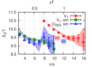
Figure 22: Fitted and local effective (cosh) masses with symbols and bands, respectively, extracted from the two-point correlation functions of the $V_{1}$, smeared $V_{1}$ and smeared $O_{\rm{35D}}$ operators with red circles, green squares and blue triangles, respectively. The short, horizontal red and blue bands show the value and error of the window-averaged masses.

Using the above definitions, we then calculated the two-point correlation function of the $O_{\rm{35D}}(x)$ operator. We performed this evaluation using also a smeared operator, which reduced the noise significantly. We also note that, similarly to the transverse screening correlators of the vector current, we performed averages over different spatial decay directions exploiting the discrete lattice rotation symmetry.

We extracted the local effective mass from the two-point function and we also performed single-state fits using a similar fit ansatz as in Eq. (32). Using the fit results for the mass, we constructed the window-smeared mass averaging fit results obtained at subsequent equal-length fit ranges. The window function was centered at $xT=0.6$ and had a width of 0.30 in this variable. These correspond to $x_{\rm{win,center}}/a\approx 7$ and a width of $3.6$ in lattice units. We note that for instance the fit results using 9 datapoints starting with $x/a=4,5,6,7,8,9,10$ have $p$-values 0.02, 0.27, 0.15, 0.18, 0.45, 0.68, 0.59, respectively, i.e. the chosen window range covers results with acceptable $p$-values. The window-averaged mass is shown by the horizontal blue bland in Fig. 22. Compared to this we also show in Fig. 22 the single-state fit results for the two-point function involving the smeared or unsmeared $V_{1}$ operator. The window-smeared mass obtained using the unsmeared $V_{1}$ is shown with the short red horizontal band in Fig. 22 and is in good agreement with the one obtained using $O_{\rm{35D}}(x)$.

In summary, while the smeared $O_{\rm{35D}}$ and $V_{1}$ correlators exhibit lower effective masses in the region $x_{3}T\lesssim 0.75$, their variance is also larger. This observation should be taken into account in future dedicated spectroscopic calculations.

References

- McLerran and Toimela (1985) L. D. McLerran and T. Toimela, Phys. Rev. D 31, 545 (1985).
- David (2020) G. David, Rept. Prog. Phys. 83, 046301 (2020), eprint 1907.08893.
- Gale et al. (2021) C. Gale, J.-F. Paquet, B. Schenke, and C. Shen (2021), eprint 2106.11216.
- Acharya et al. (2022) U. A. Acharya et al. (PHENIX) (2022), eprint 2203.17187.
- Adare et al. (2015) A. Adare et al. (PHENIX), Phys. Rev. C 91, 064904 (2015), eprint 1405.3940.
- Adam et al. (2016) J. Adam et al. (ALICE), Phys. Lett. B 754, 235 (2016), eprint 1509.07324.
- Adamczyk et al. (2017) L. Adamczyk et al. (STAR), Phys. Lett. B 770, 451 (2017), eprint 1607.01447.
- Adare et al. (2012) A. Adare et al. (PHENIX), Phys. Rev. Lett. 109, 122302 (2012), eprint 1105.4126.
- Adare et al. (2016) A. Adare et al. (PHENIX), Phys. Rev. C 94, 064901 (2016), eprint 1509.07758.
- Acharya et al. (2019) S. Acharya et al. (ALICE), Phys. Lett. B 789, 308 (2019), eprint 1805.04403.
- Geurts and Tripolt (2023) F. Geurts and R.-A. Tripolt, Prog. Part. Nucl. Phys. 128, 104004 (2023), eprint 2210.01622.
- Arnold et al. (2001a) P. B. Arnold, G. D. Moore, and L. G. Yaffe, JHEP 12, 009 (2001a), eprint hep-ph/0111107.
- Arnold et al. (2001b) P. B. Arnold, G. D. Moore, and L. G. Yaffe, JHEP 0111, 057 (2001b), eprint hep-ph/0109064.
- Paquet et al. (2016) J.-F. Paquet, C. Shen, G. S. Denicol, M. Luzum, B. Schenke, S. Jeon, and C. Gale, Phys. Rev. C 93, 044906 (2016), eprint 1509.06738.
- Turbide et al. (2004) S. Turbide, R. Rapp, and C. Gale, Phys. Rev. C 69, 014903 (2004), eprint hep-ph/0308085.
- Meyer (2011) H. B. Meyer, Eur.Phys.J. A47, 86 (2011), eprint 1104.3708.
- Aarts and Nikolaev (2021) G. Aarts and A. Nikolaev, Eur. Phys. J. A 57, 118 (2021), eprint 2008.12326.
- Backus and Gilbert (1968) G. Backus and F. Gilbert, Geophys. J. Int. 16, 169 (1968).
- Backus and Gilbert (1970) G. Backus and F. Gilbert, Philos. T. R. Soc. A 266, 123 (1970).
- Brandt et al. (2016) B. B. Brandt, A. Francis, B. Jäger, and H. B. Meyer, Phys. Rev. D 93, 054510 (2016), eprint 1512.07249.
- Hansen et al. (2017) M. T. Hansen, H. B. Meyer, and D. Robaina, Phys. Rev. D 96, 094513 (2017), eprint 1704.08993.
- Cè et al. (2022a) M. Cè, T. Harris, A. Krasniqi, H. B. Meyer, and C. Török (2022a), eprint 2211.15558.
- Cè et al. (2022b) M. Cè, T. Harris, A. Krasniqi, H. B. Meyer, and C. Török, Phys. Rev. D 106, 054501 (2022b), eprint 2205.02821.
- Altenkort et al. (2022) L. Altenkort, A. M. Eller, A. Francis, O. Kaczmarek, L. Mazur, G. D. Moore, and H.-T. Shu (2022), eprint 2211.08230.
- Astrakhantsev et al. (2020) N. Astrakhantsev, V. V. Braguta, M. D’Elia, A. Y. Kotov, A. A. Nikolaev, and F. Sanfilippo, Phys. Rev. D 102, 054516 (2020), eprint 1910.08516.
- Astrakhantsev et al. (2018) N. Y. Astrakhantsev, V. V. Braguta, and A. Y. Kotov, Phys. Rev. D 98, 054515 (2018), eprint 1804.02382.
- Alexandrou et al. (2023) C. Alexandrou et al. (Extended Twisted Mass Collaboration (ETMC)), Phys. Rev. Lett. 130, 241901 (2023), eprint 2212.08467.
- Hansen et al. (2019) M. Hansen, A. Lupo, and N. Tantalo, Phys. Rev. D 99, 094508 (2019), eprint 1903.06476.
- Bulava et al. (2022) J. Bulava, M. T. Hansen, M. W. Hansen, A. Patella, and N. Tantalo, JHEP 07, 034 (2022), eprint 2111.12774.
- Gambino et al. (2022) P. Gambino, S. Hashimoto, S. Mächler, M. Panero, F. Sanfilippo, S. Simula, A. Smecca, and N. Tantalo, JHEP 07, 083 (2022), eprint 2203.11762.
- Meyer (2018) H. B. Meyer, Eur. Phys. J. A 54, 192 (2018), eprint 1807.00781.
- Karsch and Wyld (1987) F. Karsch and H. W. Wyld, Phys. Rev. D35, 2518 (1987).
- Meyer and Wittig (2019) H. B. Meyer and H. Wittig, Prog. Part. Nucl. Phys. 104, 46 (2019), eprint 1807.09370.
- Aoyama et al. (2020) T. Aoyama et al., Phys. Rept. 887, 1 (2020), eprint 2006.04822.
- Borsanyi et al. (2021) S. Borsanyi et al., Nature 593, 51 (2021), eprint 2002.12347.
- Caron-Huot et al. (2006a) S. Caron-Huot, P. Kovtun, G. D. Moore, A. Starinets, and L. G. Yaffe, JHEP 0612, 015 (2006a), eprint hep-th/0607237.
- Brandt et al. (2014) B. B. Brandt, A. Francis, M. Laine, and H. B. Meyer, JHEP 05, 117 (2014), eprint 1404.2404.
- Ghiglieri et al. (2016) J. Ghiglieri, O. Kaczmarek, M. Laine, and F. Meyer, Phys. Rev. D94, 016005 (2016), eprint 1604.07544.
- Cè et al. (2020) M. Cè, T. Harris, H. B. Meyer, A. Steinberg, and A. Toniato, Phys. Rev. D 102, 091501 (2020), eprint 2001.03368.
- Caron-Huot et al. (2006b) S. Caron-Huot, P. Kovtun, G. D. Moore, A. Starinets, and L. G. Yaffe, JHEP 12, 015 (2006b), eprint hep-th/0607237.
- Meyer et al. (2022) H. B. Meyer, M. Cè, T. Harris, A. Toniato, and C. Török, PoS LATTICE2021, 269 (2022), eprint 2112.00450.
- Cè et al. (2021a) M. Cè, T. Harris, H. B. Meyer, and A. Toniato, JHEP 03, 035 (2021a), eprint 2012.07522.
- Dalla Brida et al. (2019) M. Dalla Brida, T. Korzec, S. Sint, and P. Vilaseca, Eur. Phys. J. C 79, 23 (2019), eprint 1808.09236.
- Fritzsch et al. (2012) P. Fritzsch, F. Knechtli, B. Leder, M. Marinkovic, S. Schaefer, R. Sommer, and F. Virotta, Nucl. Phys. B 865, 397 (2012), eprint 1205.5380.
- Luscher and Schaefer (2013) M. Luscher and S. Schaefer, Comput. Phys. Commun. 184, 519 (2013), eprint 1206.2809.
- Hasenbusch (2001) M. Hasenbusch, Phys. Lett. B 519, 177 (2001), eprint hep-lat/0107019.
- Marinkovic and Schaefer (2010) M. Marinkovic and S. Schaefer, PoS LATTICE2010, 031 (2010), eprint 1011.0911.
- Engel et al. (2015) G. P. Engel, L. Giusti, S. Lottini, and R. Sommer, Phys. Rev. Lett. 114, 112001 (2015), eprint 1406.4987.
- Cè et al. (2021b) M. Cè, T. Harris, H. B. Meyer, A. Toniato, and C. Török, JHEP 12, 215 (2021b), eprint 2106.15293.
- Akaike (1971) H. Akaike, in Petrov, B. N.; Csáki, F. (eds.), 2nd International Symposium on Information Theory, Tsahkadsor, Armenia, USSR, September 2-8 p. pp. 267–281. (1971).
- Teaney (2006) D. Teaney, Phys. Rev. D74, 045025 (2006), eprint hep-ph/0602044.
- Ghiglieri et al. (2013) J. Ghiglieri, J. Hong, A. Kurkela, E. Lu, G. D. Moore, et al., JHEP 1305, 010 (2013), eprint 1302.5970.
- Arnold et al. (2003) P. Arnold, G. D. Moore, and L. G. Yaffe, JHEP 05, 051 (2003), eprint hep-ph/0302165.
- Brandt et al. (2013) B. B. Brandt, A. Francis, H. B. Meyer, and H. Wittig, JHEP 1303, 100 (2013), eprint 1212.4200.
- Amato et al. (2013) A. Amato, G. Aarts, C. Allton, P. Giudice, S. Hands, and J.-I. Skullerud, Phys. Rev. Lett. 111, 172001 (2013), eprint 1307.6763.
- Aarts et al. (2015) G. Aarts, C. Allton, A. Amato, P. Giudice, S. Hands, and J.-I. Skullerud, JHEP 02, 186 (2015), eprint 1412.6411.
- Ding et al. (2016) H.-T. Ding, O. Kaczmarek, and F. Meyer, Phys. Rev. D94, 034504 (2016), eprint 1604.06712.
- Edwards and Joo (2005) R. G. Edwards and B. Joo (SciDAC, LHPC, UKQCD), Nucl. Phys. Proc. Suppl. 140, 832 (2005), eprint hep-lat/0409003.
- P. J. Huber (2009) E. M. R. P. J. Huber (2009).
- Braaten and Nieto (1996) E. Braaten and A. Nieto, Phys. Rev. D 53, 3421 (1996), eprint hep-ph/9510408.
- Laine and Schroder (2005) M. Laine and Y. Schroder, JHEP 03, 067 (2005), eprint hep-ph/0503061.
- Panero et al. (2014) M. Panero, K. Rummukainen, and A. Schäfer, Phys. Rev. Lett. 112, 162001 (2014), eprint 1307.5850.