Differentiable Boustrophedon Path Plans

Abstract

This paper introduces a differentiable representation for optimization of boustrophedon path plans in convex polygons, explores an additional parameter of these path plans that can be optimized, discusses the properties of this representation that can be leveraged during the optimization process, and shows that the previously published attempt at optimization of these path plans was too coarse to be practically useful. Experiments were conducted to show that this differentiable representation can reproduce the same scores from transitional discrete representations of boustrophedon path plans with high fidelity. Finally, optimization via gradient descent was attempted, but found to fail because the search space is far more non-convex than was previously considered in the literature. The wide range of applications for boustrophedon path plans means that this work has the potential to improve path planning efficiency in numerous areas of robotics including mapping and search tasks using uncrewed aerial systems, environmental sampling tasks using uncrewed marine vehicles, and agricultural tasks using ground vehicles, among numerous others applications.

I Introduction

Bostrophedon path plans, also known as raster and lawnmower path plans, can be followed by both holonomic and non-holonomic vehicles, and involve traversing an area of interest in straight lines with fixed spacing. These straight lines are referred to as transects because they transect the area of interest. These path plans are used extensively in aerial survey, environmental monitoring, and search tasks because they guarantee coverage over an area of interest.

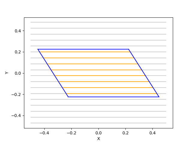
(a)

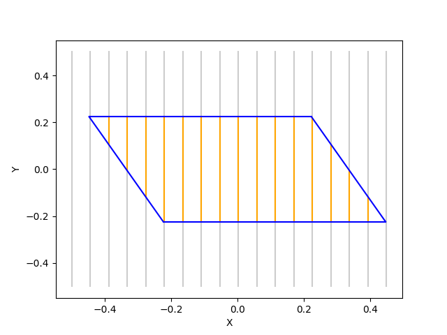
(b)

Figure 1: Transects discretely generated within a parallelogram. Transects covering the polygon are shown in yellow. Some may consider the transects in (a) to be superior to (b) as the same space is covered using a smaller count of uniform length transects.

Typically executors of these path plans start on an edge-most transect, that is followed until it terminates at the end of the area of interest whereby the next proximal transect is selected and followed in the opposite direction. This process continues until all transects have been followed. An example of these transects is depicted in yellow in Figure 1 contained within an area of interest defined using a blue parallelogram.

The literature to date exclusively represents this problem in a discrete manner by computing transects that start and end at fixed positions along the perimeter of the polygon used to define the area of interest. This approach is intuitive for robots that require discrete waypoints for use in path execution.

Recent advances in convex and non-convex optimization in machine learning have shown the effectiveness of optimization via gradient descent based methods [1]; however, this discrete representation, while convenient computationally and operationally, precludes the utilization of these methods without encumbering gradient approximation methods. At the same time, the introduction of a differentiable system for the optimization of boustrophedon path plans enables the transmission of gradients into other differentiable systems, like neural networks, which are currently unable to directly optimize these path plans.

This paper bridges this gap by presenting a numerically stable and mathematically differentiable representation for boustrophedon paths over convex polygons that enables the optimization of these paths via gradient descent. It will go on to show that this representation approximates the discrete representation with a high degree of fidelity, shows that the optimization space is more complex than previously discussed, and requires search techniques that are far more fine than the 10 degree grid search suggested in [2]. Finally it will explore the properties of this differentiable representation that can mitigate, but not fully alleviate, the issues of non-convex optimization in this space.

In addition, this paper explores the optimization of an additional parameter of boustrophedon paths. The most relevant previous work only explored the optimization of the angle of the transects[2]. However, this paper shows that shifting the transects laterally also has an impact on the fitness of a particular path solution, and that this parameter can be differentiated in the same manner as transect angle.

II Related Work

The general areas in which this work sits are well developed. Boustrophedon path planning, and its associated coverage guarantees have been extensively studied [3, 4, 5] for decades. Numerous papers, too many to cite, have explored optimization via gradient descent. Recent advances in high dimensional optimization using gradient descent have fueled, in part, major advances in machine learning [6, 1]. What differs from previous work is this paper’s focus on optimizing the length and orientation of transects.

Optimization of boustrophedon path plans have been explored before. In general Boustrophedon path plans are optimized to guarantee coverage while minimizing the total path length. However, other optimizations have been made as well. For example, the task of selecting which transect to execute next has been explored and reformulated as a variant of the traveling salesman problem [7], and as a genetic search problem [8]. However, these approaches take the transects as a given and only seek to optimize the transitions between transects in non-holonomic vehicles. This is not an issue in the case of holonomic vehicles as they have no turning rate constraints and can proceed to the next transect directly.

However, the optimization of the locations and orientations of transects has been less studied. This is important because minimizing the path length may not be an appropriate optimization in all cases. The most relevant past work in this regard is [2] which explored optimizing the angle at which a set of transects were generated for convex and concave polygons. The objective was to maximize the average length of the transects while minimizing the variance of those same transect lengths. The thought being that for sonar mapping tasks, marine vehicles would benefit from having long transects, for platform stability, with minimal variance in length to ease in sensor data interpretation. This work showed that certain orientations for these transects are favorable to others, and suggested that these orientations can be optimized using grid search. The authors evaluated the effectiveness of this method over a series of polygons that were generated by uncrewed marine vehicle operators in the field, and specifically suggest using intervals of 10 degrees to examine transect orientation. Though it should be noted that [2] only explores the optimization of a single parameter—transect orientation—on boustrophedon path fitness.

III Problem Formulation

The problem formulation is presented first as the traditional discrete approach for generating these path plans to establish a base case, followed by the differentiable approach that proposed here.

III-A Discrete Approaches

As has been discussed, boustrophedon path plans are constructed out of a set of transects that have been arranged at fixed intervals along the perimeter of the polygon. In the discrete setting, these transects are generated by iterating over the perimeter of the polygon and generating transects as appropriate. These transects are then connected along the edge of the polygon, in an alternating fashion.

An example of such a discrete set of transects is shown in Figure 1. In this figure, a field of candidate transects is generated and placed in the same space as the polygonal area of interest. The final transects are then determined by computing the intersection of these candidate transects with the polygon. This approach results in transects that are precisely the dimension of the polygon and have discrete end points.

Past work [2] then computes scores for transect orientations based on the count and dimension of the generated transects. Specifically, this work proposes the maximizing equation 1.

$$f(\theta)=a\cdot(m^{\prime}_{\theta})+b\cdot(1-COV_{\theta})$$ (1)

Where $m^{\prime}_{\theta}$ is the average length of all transects, $COV_{\theta}$ is the standard deviation of lengths of transects, and $a$ and $b$ are hyperparameters defined to weight the optimization. This optimization is over angles $\theta$ searching for a optima.

This formulation precludes differentiation because the count of the number of transects at each angle $\theta$, used to compute the mean and standard deviation, is a discontinuous function that cannot be differentiated. Formulating this problem such that a continuous function defines the count of transects in a given polygon at a given angle is the principle limiting factor.

III-B Differentiable Approach

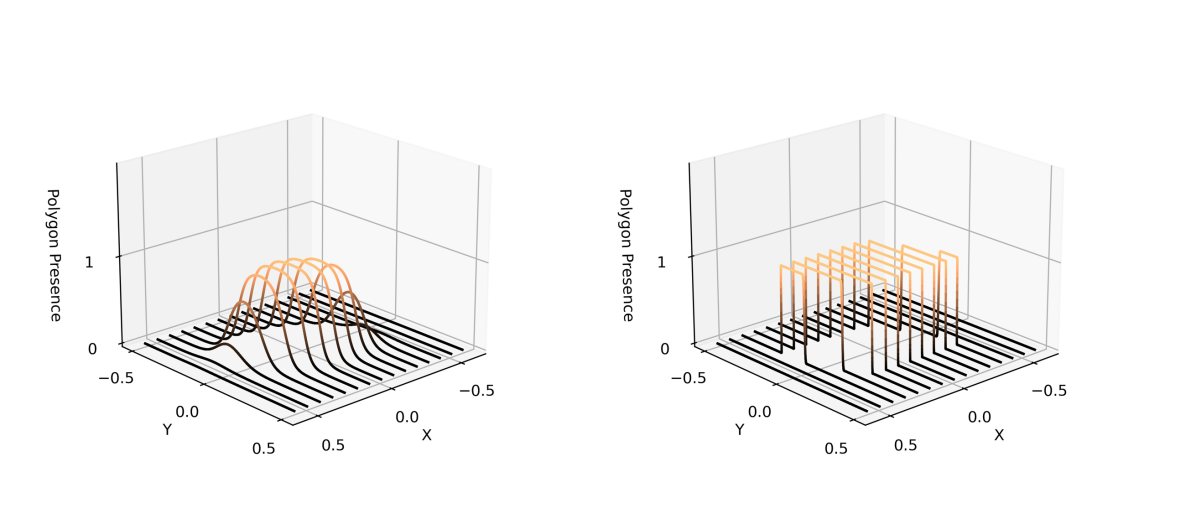
Figure 2: Transect lines passing through the parallelogram from Figure 1 using the differentiable formulation described. The z-axis corresponds to an indicator function stating if a particular point is contained within the parallelogram. Transect lengths are approximated based on the integral of these lines. Left shows Temperature=17, right shows Temperature=100.

The proposed differentiable approach similarly requires a definition for a polygon, and transects, but differs in their implementation. This section defines each of the elements necessary for evaluating a proposed polygon orientation.

III-B1 Polygon Definition

In order to come up with a differentiable function for transect fitness with respect to a given polygon, a definition of a polygon that supports differentiation must be utilized. To do this, a formulation is developed leaning on the universal approximation theorem from artificial neural networks [9]. This formulation utilizes the sum of the sigmoid of several linear functions to approximate the bounds of a polygon. More specifically, each face of a polygon is approximated using a linear function $W^{T}X+B$ where the matrix $W$ describes the slope of the edge of a polygon, $B$ describes an offset to align the edge with the rest of the polygon, and $X$ describes the point to be evaluated. The procedure for constructing $W$ and $B$ from a set of two points is straightforward. First the polygon is resized such that its maximal dimension is equal to 1, and centered on the origin. Then the $W$ and $B$ parameters of the polygon edges are defined following equation 2.

$$Given\;(x_{1},y_{1}),(x_{2},y_{2}$$ (2)

$$X_{e}=\begin{bmatrix}x_{1}&1\\ x_{2}&1\end{bmatrix}$$

$$Y_{e}=\begin{bmatrix}y_{1}&1\\ y_{2}&1\end{bmatrix}$$

$$C_{e}=\begin{bmatrix}x_{1}&y_{1}\\ x_{2}&y_{2}\end{bmatrix}$$

$$W=[Det(X_{e}),Det(Y_{e})]$$

$$B=Det(C_{e})$$

Now, each face of the polygon defined in this way is passed to a sigmoid function ($\sigma$) in order to compress it between 0 and 1 as shown in equation 3. A hyperparameter Temp, which is referred to as temperature, controls steepness of this sigmoid function. Temperature is defined as having a value (0, $+\infty$). Additional details of this hyperparameter are discussed in section VI.

$$v=W^{T}X+B$$ (3)

$$\sigma(v,Temp)=\frac{1}{1+e^{-v\cdot Temp}}$$

With this function, it can be determined if a given point is on one side of a given polygon’s edge. In order to determine if a given point is contained within a polygon, a product is taken over all of the polygon edges ($F$) as shown in equation 4.

$$P(X,F,Temp)=\prod_{(W,B)\in F}\sigma(W^{T}X+B,Temp)$$ (4)

This behaves as an approximate indicator function of whether the point $X$ is contained within the given polygon edges $F$; however, it is not numerically stable because high fidelity approximations require exceedingly high temperatures (Temp $\geq 10^{5}$). In order to combat this, the value of equation 4 is passed to another sigmoid function as shown in equation 5. This increases approximation fidelity at low temperatures, thereby preserving numerical stability.

$$P_{\sigma}(X,F,Temp)=\sigma(P(X,F,Temp)-0.5,Temp)$$ (5)

Equation 5 represents the final function that is used to approximate convex polygons. This function is entirely differentiable and provides high fidelity while being numerically stable. It should also be noted that this polygon formulation is what limits this approach to convex polygons, as it requires a point to be contained by all edges of the polygon which will only be true when there is convexity. However, [9] shows that it would be possible to extend this approach to concave polygons as well.

III-B2 Transect Definition

In order to approximate the transects, a set of lines $\gamma$ at equal width are defined. As the polygon was rescaled such that the maximum dimension was between -0.5 and 0.5, these lines run parallel to the Y axis from -0.5 to 0.5 and are repeated along the X axis at the predefined, but rescaled, spacing covering -0.5 to 0.5. Examples of these lines are shown in figure 2 and are evaluated by the polygon representation defined in section III-B1 at various temperatures.

The critical item that must be calculated in this setting is the transect length. At first glance, this appears quite difficult because of the continuous nature of the polygon defined above. However, the integral of the transect passing through the polygon can be computed to approximate the transect length. This is shown in equation 6. Defining the transects to be parallel to an axis simplifies this integral as it allows $x$ to remain constant, meaning only $y$ needs to be integrated.

$$\int_{-0.5}^{0.5}P_{\sigma}([x,y],F,Temp)dy$$ (6)

This allows us to compute the length of a single transect. This information may then be consumed by downstream differentiable scoring functions for optimization purposes.

At the time of writing, a closed form solution to the integral described in equation 6 is not known and so this integral is approximated numerically using the trapezoidal rule.

III-B3 Scoring Function Definition

With a differentiable definition of a polygon, and a formulation of transects that allows for the approximation of a transect length given a polygon, the optimization of those transects may now be discussed. With a differentiable approximation of the length of a transect, a wide variety of scoring functions can be imagined. In keeping with the literature, the fitness function from [2] in equation 1 is adapted to this setting.

To compute the average length of all transects, it must be determined if a given transect in $\gamma$ has length. To do this an additional sigmoid function is used as an indicator function for transects that have an approximated length  0. This is done as described in equation 7.

$$S(x,F,Temp)=\frac{\sigma(\int_{-0.5}^{0.5}P_{\sigma}([x,y],F,Temp)dy)-0.5}{0.5}$$ (7)

The constants $0.5$ in equation 7 are to scale the indicator function. This function will now equal 0 when the transect at $x$ has no length. With this, from equation 7, the mean and standard deviations of transect with lengths  0 can be approximated easily by using the approximated transect lengths, and the the indicator detailing if they were shown or not.

It is worth noting that while this work focuses on a differentiable implementation of the objective function presented in [2], the problem formulation described in III-B is not limited to this objective function. This approach enables a wide variety of objective functions that may be useful depending on the needs at the time. For example, in keeping with much of the literature, it may be worthwhile to simply minimize the total length of all transects, this is possible under this formulation by simply summing the approximated length of all transects. In fact, any function that has a defined derivative may be integrated into this system. Readers are encouraged to adapt and modify the scoring function described here to fit their needs.

III-B4 Computation of Gradients

As discussed in the introduction, there are two parameters for which gradients are computed: angle, and x-offset.

In the case of angle, a simplification is made compared to the previous literature [2]. Instead of rotating the transects, the polygon is rotated. This is done to simplify the computation of the integral function defined in equation 6. This is done through a simple rotational transform that is applied to $W$ and $B$ terms that rotate the edges about the origin. Gradients are then computed on the angle that is passed to this rotational transform.

In the case of x-offset, this is done by adding a parameter to the $x$ term in equation 6 and computing the gradient on that additional term.

More practically, with this problem formulation, the computation of gradients necessary for gradient descent can be readily performed by any popular auto-differentiation package. PyTorch [10] was utilized in the case of this work.

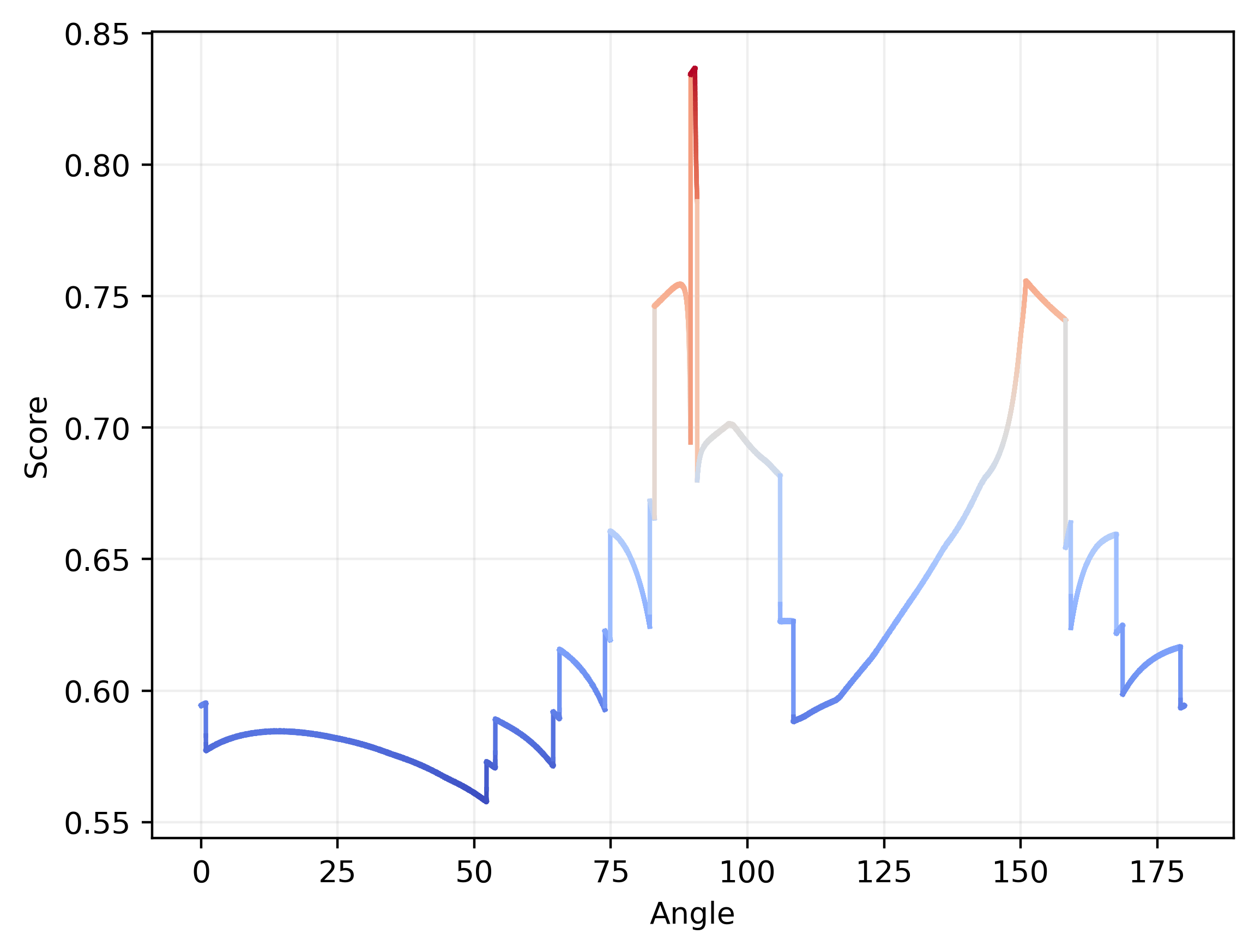
Figure 3: The score surface described by the differentiable formulation based on the parallelogram, and transects, shown in Figure 1. Here the angle is varied and the x-offset fixed at 0.0 and Temperature at 10000.

IV Comparison with Discrete Representations

An obvious question that follows this complex mathematical machinery is if it does a sufficient job of approximating the discrete formulation. In order to answer this question, an experiment was conducted where random orientations, x-offsets, transect spacings, and convex polygons with sides $[3,10)$ were generated. These parameters were then passed to a discrete system where the transect lengths, and subsequent fitness scores, were computed precisely, and the differentiable system where the fitness scores were approximated. Both of these fitness scores were measured and absolute differences were computed. In this context, the discrete implementation is considered truth, and any deviation from the discrete score is considered error. In this experiment, the fitness function from [2] and shown in equation 1 was used, resulting in a bounded score between 0 and 1. For additional context, the temperature and the number of points used to approximate the integral in equation 6 was varied and for each variation 1000 samples were taken. The results of this experiment can be found in Table I.

Error	100 PPT	1000 PPT	10000 PPT
Temperature=1	0.50798	0.50795	0.50408
Temperature=10	0.08480	0.08369	0.08367
Temperature=100	0.03090	0.03001	0.03167
Temperature=1000	0.00374	0.00271	0.00306
Temperature=10000	0.00203	0.00055	0.00016

TABLE I: Average error between discrete and differentiable scores when comparing temperature, and points per transect (PPT).

As seen in this table, as the temperature and number of points used to approximate the integral grow, the error decreases. Minimally the error was observed to be 0.00016 on a fitness function bounded between 0-1. It is argued that this corresponds to a high degree of fidelity and that this is sufficiently accurate for the optimization tasks presented in [2].

In addition, it should be noted that while increasing the temperature beyond the ranges of this table may increase precision, it may also lead to numerical instability due to overflow of the floating point representation. At the same time, while increasing the points per transect does increase the fidelity of the representation by increasing the resolution of equation 6, it also increases run-time.

V Discussion of the Optimization Space

With reasonable parity between the discrete and differentiable representations, discussion turns to the nature of the optimization space. Taking the example shown in figure 1, figure 3 shows the optimization surface generated when varying the angle and keeping the x-offset fixed. Even in this simple polygon with a low number of transects there is intense non-convexity. This non-convexity is not a function of the differentiable representation as there is very close parity between the discrete and differentiable representations at this scale. Instead, this non-convexity is due to the fact that there are fewer transects visible in some orientations of the polygon than others. As the polygon rotates, some transects leave the volume of the polygon. This leads to gradual decreases in the fitness as the transects become smaller, and then a rapid increase in fitness as the smaller outlier transect is removed from the pool of visible transects.

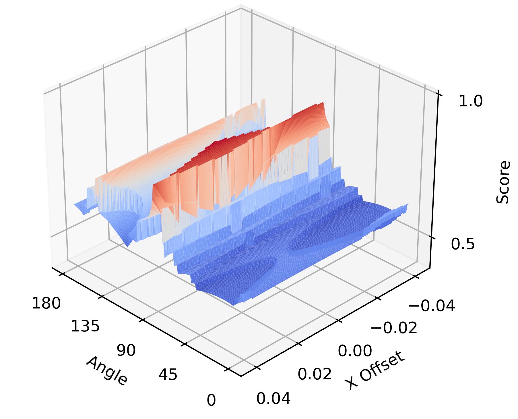
Figure 4: The 2D score surface described by the differentiable formulation based on the parallelogram, and transects, shown in Figure 1. Here the angle and the x-offset are varied. The slice where x-offset is equal to 0.0 is displayed in Figure 3.

Further optimization surface complexity is observed when varying the x-offset variable. In figure 4, again utilizing the polygon and settings from figure 1, the optimization surface of both the angle and the x-offset is shown. While the complexity of the x-offset axis appears lesser than that of the angle axis, it no doubt has an impact on the shape of the optimization surface meaning that it needs to be considered in future optimization efforts.

The intense non-convexity of this optimization surface means that future efforts in searching these spaces need to operate at a far more fine grained resolution than the 10 degree interval suggested in [2].

There are two main factors that drive this non-convexity: transect spacing, and polygon aspect. In the case of transect spacing, as transect spacing decreases and the transect count increases, the non-convexity of the function increases because the rate at which transects will be entering and exiting the polygons volume will increase. In the case of polygon aspect, polygons with a high aspect ratio will have more non-convex loss surfaces because as the polygon rotates, more transects will enter and exit the polygon’s volume. While a circle, or a shape with an aspect ratio of 1, would have a uniform loss surface as any orientation would be equally as fit. These two factors play together to create the non-convex nature of the optimization surface.

VI Discussion of Temperature

Temperature is the only hyperparameter that is introduced in this representation and as a result it is worth discussing its properties. The temperature can be seen as a parameter which governs discreteness of transect lengths. At high temperatures, the transect lengths are approximated with greater fidelity, and therefore discreteness, than at lower temperatures. When viewing a single transect, increasing the temperature can be seen as discretizing the transect, however, the effect is more intuitive when thinking about the polygon as a whole. From the perspective of the polygon, lowering the temperature “melts” the polygon, and raising the temperature solidifies it, a visual depiction of this is shown in figure 2.

From the perspective of the loss surface, it has the same effect. The loss surface becomes far smoother and undulating at lower temperatures than at high temperatures. This is shown in figure 5, where the temperature is varied in conjunction with the angle. It should be noted that while gradients can also be computed for the temperature, it is not recommended to optimize this parameter directly as it impacts the fidelity of the representation and optimizers may find themselves trapped in temperature based optima.

However, it may be beneficial to vary the temperature depending on the progress of the optimization. For example, one could perform gradient descent in a low temperature setting initially, leveraging the smoother loss surface, and then increase the temperature to increase the fidelity and refine the optima later on in the optimization process.

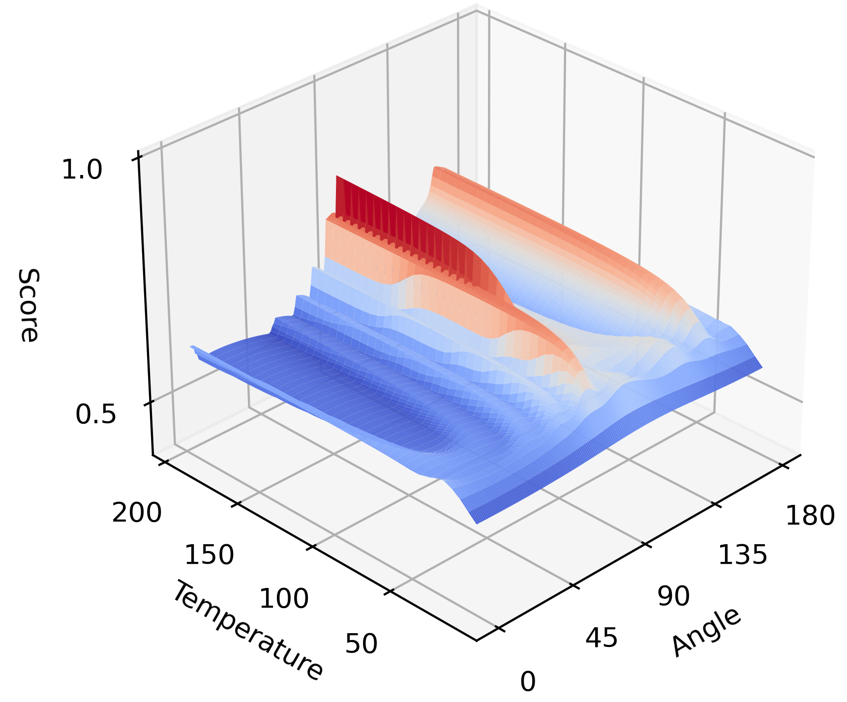
Figure 5: The 2D score surface described by the differentiable formulation based on the parallelogram, and transects, shown in Figure 1. Here the angle and temperature are varied. While this figure only shows temperatures less than 200, the slice where the temperature is equal to 10000 is displayed in Figure 3.

VII Optimization via Gradient Descent

As discussed previously, the loss surface is intensely non-convex with numerous local optima and only a single global optima. This presents a very difficult optimization space to work in as it can be impossible to know if you have reached the global minima with confidence.

To highlight this difficulty, an experiment was conducted which provided both grid search and a gradient descent approach the chance to optimize 1000 randomly generated convex polygons, generated in the manner as the experiment in section IV. In this experiment, gradient descent with a momentum of 0.8 was used. It was found that on average, grid search arrived at an an optima that was 0.13633 higher than that of the gradient descent based approach, though gradient descent did occasionally converge to an optima greater than that suggested by grid search. This is unsurprising given the intense non-convexity observed in this loss surface as shown in figures 3, 4, and 5.

This result highlights how much more non-convex this optimization space is than was previously thought. Further it represents the well known fact that optimization in non-convex spaces remains a difficult problem, and the tradeoffs between gradient descent and grid search proceed in the usual way. This work should not be seen as a solution to the non-convexity presented by this problem, but instead as another tool that may be used to improve optimization efforts in this difficult setting.

It is theorized that the best chance of arriving at the global optima efficiently in this setting will be through a combination of grid search and gradient descent where grid search will be utilized to arrive at a parameterization near to the global optima, and gradient descent will be used to refine that optima.

VIII Conclusions

While optimization via gradient descent remains difficult due to the intense non-convexity found in the loss surface, the analysis in this paper demonstrates that optimization via gradient descent can provide utility as a mechanism to further refine solutions generated via grid search. The results show that a differentiable implementation of boustrophedon path plans over convex polygons approximates the discrete formulation commonly used with a high degree of fidelity that can be tuned depending on the needs of the optimization problem. It also shows that the optimization surface is far more non-convex than previously discussed in the literature motivating the need for far more fine grained search methods than previously discussed. From a broader perspective, this work contributes to understanding the the details of the optimization space, especially providing an explanation for the non-convexity, the utility of the temperature hyperparameter in the differentiable representation, and the use of gradient descent to optimize path plans.

Future work in this space will focus on two elements: first, the development of a closed form solution to the integral in equation 6; and second, the refinement of optimization strategies that utilize gradient descent and grid search to arrive at more precise optima. The development of a closed form solution to the integral in equation 6 would result in a speed up factor equivalent to the number of points per transect that are used to empirically calculate the integral.

References

- [1] T. J. Sejnowski, “The unreasonable effectiveness of deep learning in artificial intelligence,” Proceedings of the National Academy of Sciences, vol. 117, no. 48, pp. 30 033–30 038, 2020.
- [2] T. Smith, S. Mukhopadhyay, R. R. Murphy, T. Manzini, and I. Rodriguez, “Path coverage optimization for usv with side scan sonar for victim recovery,” in 2022 IEEE International Symposium on Safety, Security, and Rescue Robotics (SSRR). IEEE, 2022, pp. 160–165.
- [3] H. Choset and P. Pignon, “Coverage path planning: The boustrophedon cellular decomposition,” in Field and service robotics. Springer, 1998, pp. 203–209.
- [4] H. Choset, “Coverage of known spaces: The boustrophedon cellular decomposition,” Autonomous Robots, vol. 9, pp. 247–253, 2000.
- [5] ——, “Coverage for robotics–a survey of recent results,” Annals of mathematics and artificial intelligence, vol. 31, pp. 113–126, 2001.
- [6] S. Ruder, “An overview of gradient descent optimization algorithms,” arXiv preprint arXiv:1609.04747, 2016.
- [7] R. Bähnemann, N. Lawrance, J. J. Chung, M. Pantic, R. Siegwart, and J. Nieto, “Revisiting boustrophedon coverage path planning as a generalized traveling salesman problem,” in Field and Service Robotics: Results of the 12th International Conference. Springer, 2021, pp. 277–290.
- [8] J. Yuan, Z. Liu, Y. Lian, L. Chen, Q. An, L. Wang, and B. Ma, “Global optimization of uav area coverage path planning based on good point set and genetic algorithm,” Aerospace, vol. 9, no. 2, p. 86, 2022.
- [9] G. Cybenko, “Approximation by superpositions of a sigmoidal function,” Mathematics of control, signals and systems, vol. 2, no. 4, pp. 303–314, 1989.
- [10] A. Paszke, S. Gross, F. Massa, A. Lerer, J. Bradbury, G. Chanan, T. Killeen, Z. Lin, N. Gimelshein, L. Antiga, A. Desmaison, A. Kopf, E. Yang, Z. DeVito, M. Raison, A. Tejani, S. Chilamkurthy, B. Steiner, L. Fang, J. Bai, and S. Chintala, “Pytorch: An imperative style, high-performance deep learning library,” in Advances in Neural Information Processing Systems 32. Curran Associates, Inc., 2019, pp. 8024–8035. [Online]. Available: http://papers.neurips.cc/paper/9015-pytorch-an-imperative-style-high-performance-deep-learning-library.pdf