DynaPix SLAM: A Pixel-Based Dynamic SLAM Approach

Abstract

In static environments, visual simultaneous localization and mapping (V-SLAM) methods achieve remarkable performance. However, moving objects severely affect core modules of such systems like state estimation and loop closure detection. To address this, dynamic SLAM approaches often use semantic information, geometric constraints, or optical flow to mask features associated with dynamic entities. These are limited by various factors such as a dependency on the quality of the underlying method, poor generalization to unknown or unexpected moving objects, and often produce noisy results, e.g. by masking static but movable objects or making use of predefined thresholds. In this paper, to address these trade-offs, we introduce a novel visual SLAM system, DynaPix, based on per-pixel motion probability values. Our approach consists of a new semantic-free probabilistic pixel-wise motion estimation module and an improved pose optimization process. Our per-pixel motion probability estimation combines a novel static background differencing method on both images and optical flows from splatted frames. DynaPix fully integrates those motion probabilities into both map point selection and weighted bundle adjustment within the tracking and optimization modules of ORB-SLAM2. We evaluate DynaPix against ORB-SLAM2 and DynaSLAM on both GRADE and TUM-RGBD datasets, obtaining lower errors and longer trajectory tracking times. We will release both source code and data upon acceptance of this work.

1 Introduction

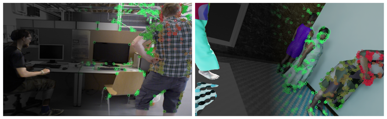
Figure 1: Examples of DynaPix motion probabilities on TUM-RGBD (left) and GRADE (right). On the left side of each image we highlight selected moving regions, e.g. partial body and shadows, and on the right side the feature’s motion probability values are passed to the SLAM system. The green color represents static features while red represents the dynamic ones.

Visual Simultaneous Localization and Mapping (V-SLAM) algorithms have undergone significant development [13] and found wide-ranging applications in various scenarios, including indoor service robots [47], urban autonomous vehicles [10], and augmented reality devices [28]. Classic visual SLAM frameworks [38, 14, 21] have been developed under a static-world assumption [44, 58]. However, since the presence of moving objects often leads to degradation in both estimation accuracy and system robustness [8, 12, 47], their widespread deployment in general real-world scenarios is limited. SLAM methods that work in dynamic environments (dynamic SLAM) often introduce visual feature removal procedures based on a prior definition of movable object classes [3, 60, 63]. However, relying on an a-priori categorization heavily restricts the generalization of SLAM systems [48, 46] due to their dependency on both the quality of underlying networks and the pre-selection of movable object classes. Then, while actually moving objects not belonging to those classes continue to degrade performance, the ones belonging to them are blindly masked. To address that, several works apply optical flow [62, 34], depth clustering [45, 31, 61], or learning-based methods [46, 6] to identify dynamic regions. However, this classification is driven by the underlying estimation of those measurements. Those are often noisy in the presence of imperfect sensors or indoor and highly dynamic environments. This leads to possible misclassifications, especially when adopting thresholds to identify dynamic objects. Methods that combine geometric and semantic information to increase robustness [31, 24, 17] still heavily rely on prior semantic clues to exclude dynamic regions surrounding selected object classes, while are still incapable of detecting other moving objects. Moreover, these approaches fail to detect either shadows or reflections and aim to completely mask objects without considering if just part of them might be slightly moving or completely static. This, while adopting binary masks instead of blended probability distributions, thus effectively discarding potentially useful information.

To solve the above problems, we propose a novel visual SLAM system based on a pixel-wise motion probability estimation for indoor dynamic environments, DynaPix. In the first stage, our system adopts a novel static/dynamic background and optical flow differencing method to obtain the motion probability of every pixel in the image without relying on semantic information. While the background can be either synthetically generated or obtained through inpainting methods, the optical flow is obtained after splatting-based view synthesis. This module is designed to be more general and can effectively capture the movements of shadows, reflections, and object parts. The estimated probability is then applied in the map points selection procedure and into a novel weighted bundle adjustment (weighted BA) in both the tracking and backend optimization modules of ORB-SLAM2. These modifications effectively reduce the influence of dynamic factors. To evaluate our method, we apply our enhanced versions of DynaSLAM [3] and its underlying SLAM framework, ORB-SLAM2 [38], on both TUM-RGBD [49] and GRADE [8] datasets, evaluating them on the absolute trajectory error (ATE) metric and the actual amount of tracking time for each experiment. We demonstrate that our approach achieves both lower trajectory errors with higher tracking times in most cases. We release both our source code and data as open source.

2 Related Work

In this section, we first briefly review various SLAM-oriented motion segmentation techniques, and then the current landscape in dynamic V-SLAM.

Motion Segmentation: Motion segmentation aims to identify the independently moving objects (pixels) from the current image frame [41]. Typical approaches apply geometric constraints to eliminate dominant motion in the image due to the camera movement, and then cluster regions that follow different rigid transformations [36]. These often consist of motion detection on depth clusters [26, 61], multi-view epipolar geometry [18], or optical-flow-based methods [5, 34]. However, such approaches often rely on pre-defined thresholds as detection criteria [59] and are incapable of adapting to different environments [12]. Moreover, the errors derived from noisy flow estimation or geometric clues in the presence of camera movement or featureless image parts can further degrade the accuracy of moving object identification. Learning-based flow estimation networks [50, 20] have also been investigated to detect moving objects [15, 11, 19, 53]. Existing methods often rely either on appearance cues or on salient motions from 2D optical flow to segment moving regions in the image frame. However, they tend to classify foreground objects wrongly as moving, especially in the presence of camera motion, and seek to identify the objects as a whole even if only some parts of them are moving, while still using binary representations. Utilizing semantic information obtained by deep neural networks (DNN) to detect or segment moving objects belonging to pre-defined categories is also a strategy that is being adopted in the literature [3, 60, 63, 27, 31]. However, apart from their inability to detect shadows and reflections, these approaches often present poor generalization capabilities due to their usage of predefined categories [46]. Additionally, they will incorrectly mask both completely static objects (e.g. parked cars) and the entirety of partially moving ones [24] (e.g. humans).

Methods consisting of a combination of geometric constraints, semantic information, and/or flow estimation like Rigid Mask [59], Flownet3D [33], or Competitive Collaboration [42], still apply a trade-off in identifying moving regions by using prior segmentation information [59], full pointclouds [33] information, and are often based on learning-based frameworks that are highly dependent on the data used [33, 59, 42]. Moreover, most of them are being tested only in outdoor scenarios where the majority of the data points are arguably static, possibly limiting their usability in indoor dynamic scenes. Finally, they still focus on identifying object instances rather than actually moving parts of the frame, while providing binary masks as output of their methods instead of blended probabilities.

Differing from prior work, we do not use any pre-defined threshold over which everything is considered to be equally dynamic, and/or segmentation class. Moreover, by using the background information, we can identify shadows and reflections. The combination of that with optical flow information based on a splatted view allows us to generate a moving probability distribution for each pixel rather than simply masking instances of objects in the image.

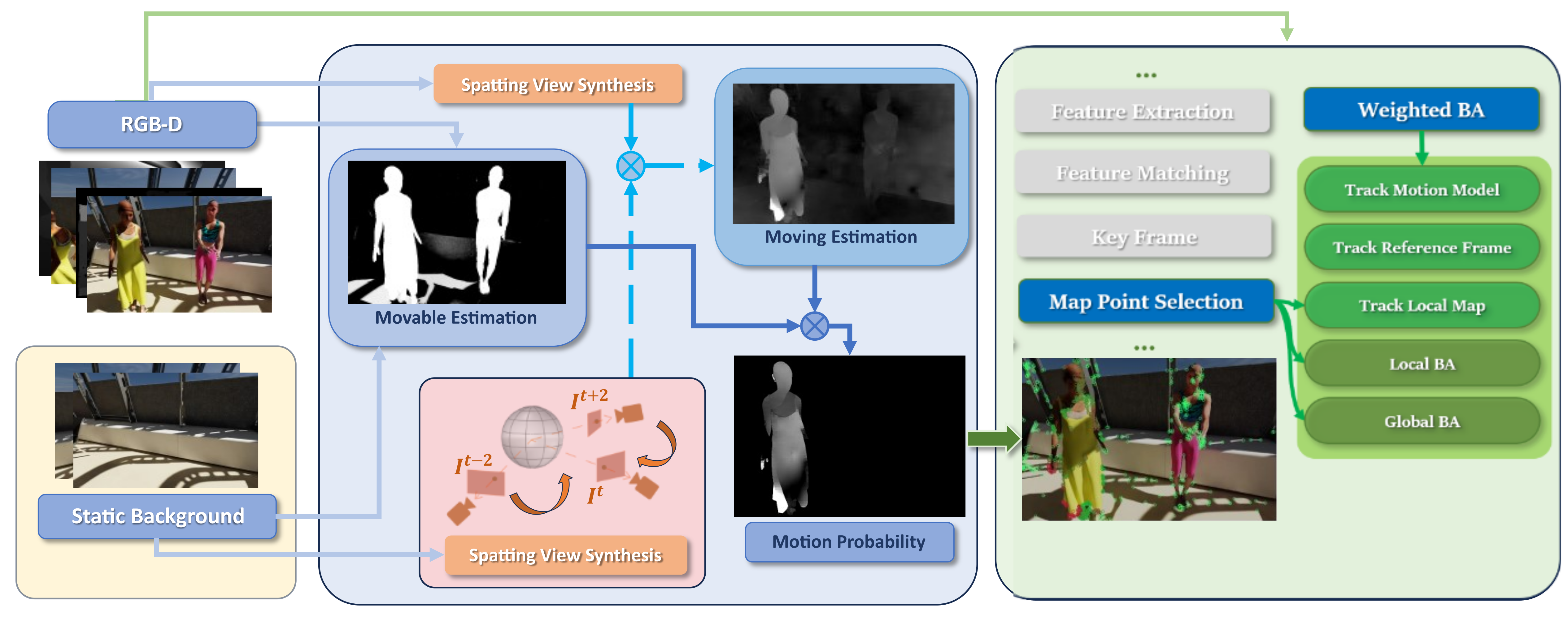
Figure 2: The DynaPix architecture consist of two main blocks, the motion probability estimation (blue box), and the modified ORB-SLAM2 (green box). We use RGB-D and corresponding background images to extract movable (Sec. 3.1.1) and moving regions (Sec. 3.1.2) on the current frame. The estimated moving probabilities are then integrated into all colored blocks of our SLAM backend (Sec. 3.2).

Dynamic V-SLAM: Most Dynamic V-SLAM methods are de-facto enhanced versions of classic SLAM frameworks [38, 14, 21, 40] combined with motion segmentation techniques. The dynamic regions are then separately tracked [54, 2, 4] or discarded as outliers [3, 60, 63, 29, 16, 56] to reduce the negative effects in pose estimation. DynaSLAM [3], for example, combines Mask R-CNN [23] and multi-view geometry to process moving objects, while DS-SLAM [60] applies a lightweight SegNet [1] to obtain segmented masks. Similarly, Detect-SLAM [63] uses SSD [32] for object detection in keyframes, whereas YOLO-SLAM [57] employs YOLOv3 [43] as its underlying detection module to identify dynamic regions. However, these methods pay less attention to the actual motion states of the detected objects, easily leading to few features retained and degradation in static scenes with frequent wrong detections, thus further degrading the system performance and causing possible failures [8]. Instead of extracting semantic information, DymSLAM [54] applies multi-motion fitting to segment different moving objects to estimate the motion of both camera and moving objects. Lu et al. [35] combine dense optical flow with depth information to generate scene flow masks to capture dynamic regions, while Flowfusion [62] uses optical flow residuals to highlight dynamic regions in RGB-D point clouds. DytanVO [46] proposes an iterative framework to jointly refine both ego-motion estimation and motion segmentation. While effectively overcoming the reliance on semantic information, these methods are heavily restricted by noise sensitivity and difficult to deploy in real-world scenes.

Methods that integrate motion probability normally fuse the semantic attributes with the motion attributes. Detect-SLAM [63] introduces the propagation of motion probability derived from object detection, while DP-SLAM [29] and Cheng et al. [16] put forward dynamic region removal techniques within the Bayesian framework to enhance motion probability updates. All of these methods, however, eliminate the dynamic features with a threshold-based filter and do not retain motion probabilities. Close to our work, [24, 64, 22] use the motion probability as a weight in the bundle adjustment (BA) procedure. However, the weighting is directly discounted in the optimization, making it irrelevant after some iterations, and is only used within the tracking module of ORB-SLAM2. As opposed to that, we do not discount or optimize this factor while propagating probabilities throughout the entire SLAM framework.

3 Approach

The goal of this work is to obtain a robust visual SLAM system in indoor dynamic environments, which consists of two novel core modules: a pixel-wise motion probability estimator and an enhanced pose optimization process. Fig. 2 briefly demonstrates our proposed DynaPix SLAM system. We first take RGB-D sequences and static background images as system inputs. The background images can be either synthetically generated [8] or inpainted through various state-of-the-art techniques [3, 30, 37]. Then, we decouple the pixel motion probability estimation process (Sec. 3.1) into two stages, which use a combination of corresponding background images and adjacent frames to produce the desired distribution. These modules consider the motion of shadows or reflections in the environment and are capable of detecting specific moving parts of deformable objects, as can be seen in Fig. 2. With the usage of probabilistic motion information, useful features are then retained throughout the estimation pipeline, rather than getting blindly discarded by the usage of binary masks. To incorporate these motion probabilities into the pose optimization process of the SLAM backend, a series of modifications are introduced in ORB-SLAM2. These include a map point selection process (Sec. 3.2.1) and a weighted-BA (Sec. 3.2.2) acting in both the tracking, and the local and global BA backend optimization modules. Details of each step of the pipeline are presented in the following sections.

3.1 Pixel-wise Motion Probability

Before proceeding, we make a distinction between movable regions, i.e. potential dynamic regions or regions in the frame where motion can occur, and moving regions, i.e. regions which are actually moving or about to move in the current frame. The goal of this module is to estimate moving regions in the current image frame using assigned probability values in place of binary masks.

As discussed in Sec. 2, learning-based flow estimation networks [50, 20] are commonly used to identify moving regions. However, the deployment in indoor dynamic environments poses specific challenges, including increased false correspondences in textureless areas (e.g. empty walls, floors), noisy estimation due to incomplete elimination of camera motion, and misclassification of foreground objects. To address these issues, our proposed probabilistic motion estimation is composed of two submodules: movable region (Sec. 3.1.1) and moving region estimation (Sec. 3.1.2). Movable regions are computed through background differencing and generate distributions covering potential moving objects with the corresponding shadows/reflections. Moving regions are then estimated through a rectified flow differencing mechanism which uses a novel combination of splatting view synthesis and static background with dynamic flow subtraction. The two are then fused (Sec. 3.1.3) to obtain the final pixel-wise motion probability. With this estimator, we manage to overcome general shortcomings of classic semantic-based detectors, such as imprecise detection/segmentation or limitation to predefined categories, while successfully reducing the estimated errors due to the direct usage of optical flow methods.

3.1.1 Movable Region Distribution Estimation

The movable distribution estimation serves as prior confidence to estimate motion attributes on the current frame. The static background images used in the differencing process can be either synthetically generated for simulated scenes by removing all potentially dynamic objects from the scene, or inpainted using E2FGVI [30] for real-world sequences. Making use of static background images, we observe that the difference between dynamic scenes and static scenes can provide reliable information about where the motion may occur, especially by capturing shadows and reflections that affect the environment. Indeed, the presence of such dynamic objects not only occludes the static background in the frame with the object itself, but brings variations to the surroundings by influencing the lighting conditions. Therefore, we subtract to the observed RGB frame (in dynamic scenes) $I$ the corresponding static frame $I_{bg}$:

$$I_{diff}(x,y)=|I(x,y)-I_{bg}(x,y)|\in[0,255]^{3}$$ (1)

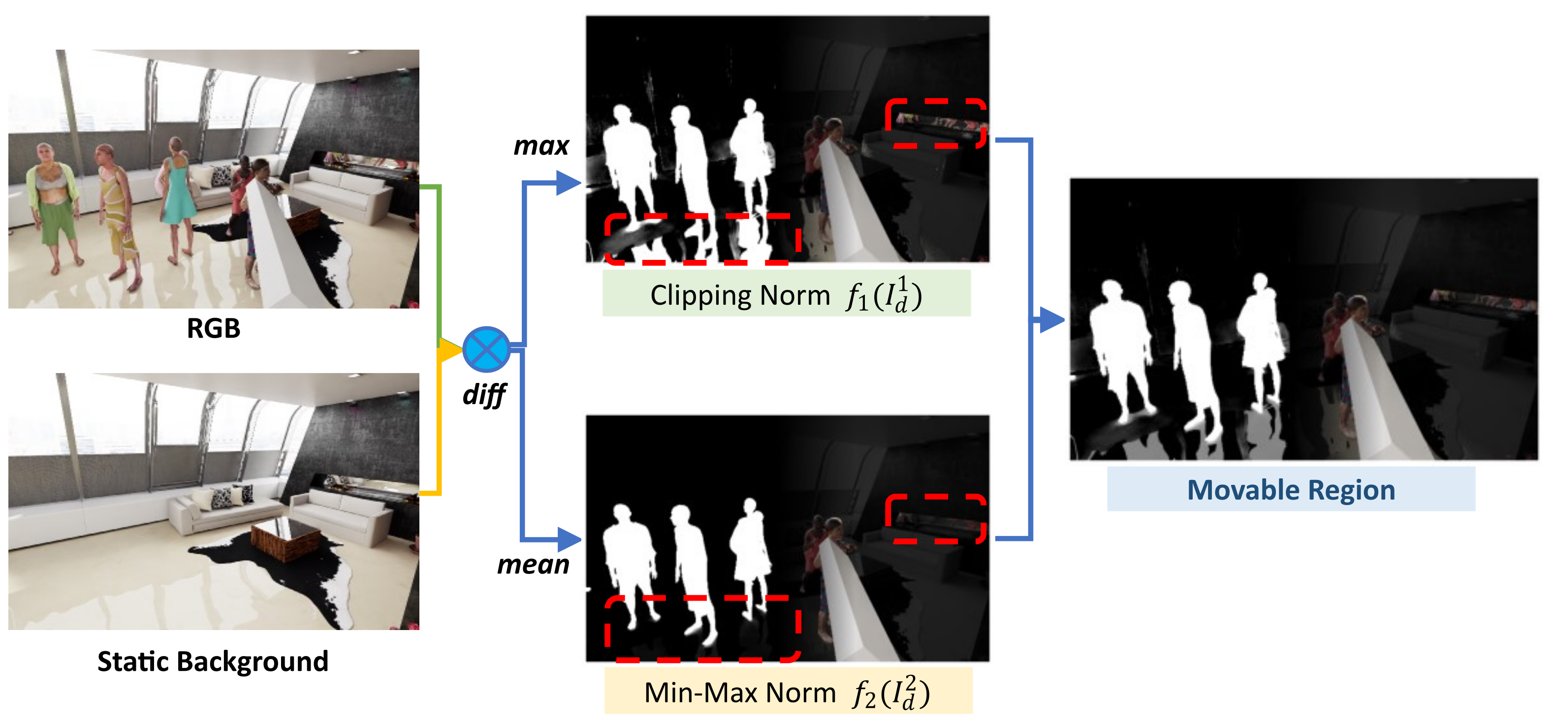
Figure 3: The process of probability estimation of movable regions. From the left: inputs, applied transformations, and results.

$I_{diff}(x,y)$ is the absolute difference of RGB image $I$ and static background image $I_{bg}$ at location $(x,y)$ over RGB color channels. We then apply $I^{1}_{d}$ and $I^{2}_{d}$ to represent $I_{diff}$ as, respectively, the maximum and the average value of the pixel at that location:

$$\begin{split}I^{1}_{d}(x,y)&=\mbox{max}(I_{diff}(x,y))\\ I^{2}_{d}(x,y)&=\mbox{mean}(I_{diff}(x,y))\\ \end{split}$$ (2)

The movable probability for any pixel, $p_{m}$, is then computed with these two terms through:

$$\begin{split}p_{m}&=\lambda\cdot f_{1}(I^{1}_{d})+(1-\lambda)\cdot f_{2}(I^{2}_{d})\\ \end{split}$$ (3)

where $f_{1}$ and $f_{2}$ are scaling methods to project $I^{1}_{d}$ and $I^{2}_{d}$ to $[0,1]$. $f_{1}$ applies clipping normalization over the specific interval, in our case $[15,35]$. This is used to define an interval to reduce the effect of noise, change of illumination, and similar factors that can influence the RGB values of corresponding frames. $f_{2}$ adopts a min-max normalization within the current frame. $\lambda$ is used to weight the two terms, and can be expressed as:

$$\begin{split}\lambda=\frac{1}{2}+\frac{1}{\mbox{exp}(0.04\cdot\mbox{max}(I^{2}_{d}))+1}\in[0,1]\end{split}$$ (4)

$\lambda$ is necessary because any given RGB frame, $I$, may be relative to a scene without any movable objects. The image would then be highly similar to the corresponding static background image, $I_{bg}$. Applying then $f_{2}$ to the difference between the two would cause exploding factors due to the min-max normalization. The formulation can effectively reduce this effect by adjusting the participation of two terms.

With the combination of $f_{1}$ and $f_{2}$, the movable regions can be captured within a probabilistic distribution. In Fig. 3, we can observe that the first term $f_{1}$ is better at capturing unnoticeable variations including shadows and reflections, while $f_{2}$ can effectively reduce noise/error.

3.1.2 Moving Region Estimation

To determine the pixel-wise motion attributes, the problem can be formulated as the pixel displacement across the frames in 3D Euclidean space. This displacement can be further projected to the current 2D image frame for observations. The neighboring frames are reprojected to the current view to eliminate camera motion. Then, we adopt FlowFormer [25] as our underlying optical flow estimation module to provide correspondences for pixel-wise moving estimation. Ideally, when comparing the current frame with the reprojected frame, the static pixels should remain at the same coordinates, while the moving pixels show obvious displacements. This can be expressed as follows:

$$\begin{split}I^{t}(x,y)=\begin{cases}\mbox{static}&\mbox{if}\quad\mbox{dist}=\sqrt{||x-x^{\prime}||^{2}+||y-y^{\prime}||^{2}}\approx 0\\ \mbox{moving}&\mbox{else}\\ \end{cases}\end{split}$$ (5)

where $t$ denotes the frame timestamp, and $(x^{\prime},y^{\prime})$, represents the coordinates of the matched pixel in the reprojected frame. However, this expression requires further corrections when considering the incomplete elimination of camera motion and false pixel correspondences across the frames. Hence, we propose splatting-based view synthesis for accurate projection, and static/dynamic flow differencing for reliable moving region estimation.

Splatting-based View Synthesis. The goal is to synthesize image observations from other viewpoints to the corresponding location. The common approach adopts homography transforms to perform image reprojection [51, 52]. However, these transformations assume that the observed points belong to the same plane regardless of their depth information. This clearly causes displacements between the current frame $I^{t}$ and the reprojected frame $\widetilde{I}^{t+i}$. To overcome this we follow the idea of softmax splatting [39] for more accurate view synthesis.

Given camera intrinsic matrix $K$, depth map at adjacent frame $Z^{t+i}$, we project the pixels of frame $I^{t+i}$ into 3D space to recover their 3D information, then reproject these 3D points $\textbf{X}^{t+i}$ to the current viewpoint with an initially estimated transformation $\{R,\textbf{t}\}$:

$$\begin{split}&\textbf{X}^{t+i}=K^{-1}\textbf{x}^{t+i}Z^{t+i}\\ &\widetilde{\textbf{x}}^{t+i}=K(RK^{-1}\textbf{X}^{t+i}+\textbf{t})\end{split}$$ (6)

where x denotes the 2D pixel coordinates, and $\widetilde{\textbf{x}}^{t+i}$ represents the reprojected coordinate for each pixel at frame $\widetilde{I}^{t+i}$ when observing from the current viewpoint.

With these prior correspondences between the frame $I^{t+i}$ and the desired transformed frame $\widetilde{I}^{t+i}$, each pixel in the frame $\widetilde{I}^{t+i}$ is synthesized by participation from adjacent pixels, which can be expressed as:

$$\begin{split}\widetilde{I}^{t+i}(x,y)=\frac{\vec{\Sigma}(\mbox{exp}(z^{\prime})\cdot I^{t+i}(x^{\prime},y^{\prime}))}{\vec{\Sigma}(\mbox{exp}(z^{\prime}))}\end{split}$$ (7)

where $\vec{\Sigma}(\cdot)$ denotes the summation of all contributed pixels from the original frame $I^{t+i}$, $\mbox{exp}(z^{\prime})$ serves as the weight in this summation which relates to the depth of each pixel in frame $I^{t+i}$, and $(x^{\prime},y^{\prime})$ represents the corresponding coordinates of contributed pixels in $I^{t+i}$. More details can be found in [39]. In Fig. 4, we show the advantage of using splatted views over homography transforms.

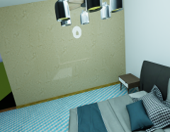
(a) Frame $I^{t}$

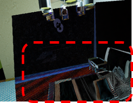
(b) Homography TF

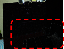
(c) Soft Splatting

Figure 4: Frame difference between a reprojected frame $\widetilde{I}^{t+i}$ and Frame $I^{t}$. While there is evident noise when subtracting a homography-transformed image, using the splatted view synthesis achieves noise-free results.

Differencing Flow for Moving Estimation. Having obtained the reprojected view $\widetilde{I}^{t+i}$ from the splatting synthesis module, the static regions can be aligned correctly to the current view ${I}^{t}$. At this stage, the moving region estimation can be simply formulated as the flow estimation between these two frames by $\mathcal{F}({I}^{t},\widetilde{I}^{t+i})$, where the distance between each correspondence in Eq. 5 can be represented by flow magnitudes. This, despite displaying considerable effects in reducing errors, can not completely remove either the camera motion effects or false pixel correspondences that frequently occur in texture-less and ambiguous texture-rich areas during the flow estimation process. As shown in Sec. 2, those common problems are observed in current state-of-the-art methods. Interestingly, we observe a similar distribution of errors when performing flow estimation only on static background images. Therefore, we apply the flow estimation on static backgrounds as well, using the same procedure explained above, to further compensate for the errors in the same regions through:

$$\begin{split}\mathcal{M}(I^{t},\widetilde{I}^{t+i})=\mbox{min}(\mathcal{F}({I}^{t},\widetilde{I}^{t+i}),\mathcal{F}({I}^{t},\widetilde{I}^{t+i})-\mathcal{F}({I}_{bg}^{t},\widetilde{I}_{bg}^{t+i}))\\ \end{split}$$ (8)

where $\mathcal{M}(I^{t},\widetilde{I}^{t+i})$ is the distribution of flow magnitudes over the frame. The low-pass filter is applied to avoid higher flow magnitudes due to subtraction on noisy estimations.

3.1.3 Final Motion Probability

Assuming that motion is consistent over a short period of time, the motion attribute of each pixel should be similar or little varying in the neighboring frames. Therefore, we finalize the moving region estimation at the current frame $\mathcal{M}^{t}$ across multiple frames:

$$\begin{split}\mathcal{M}^{t}&=\frac{1}{2n}\sum_{j\in J}\left(\mathcal{M}({I}^{t},\widetilde{I}^{t+j})+\mathcal{M}({I}^{t},\widetilde{I}^{t-j})\right)\end{split}$$ (9)

Where $J$ is a set of time offsets and $n$ is its cardinality. We adopt $J=[2]$ in our implementation to represent the moving region estimation at the frame $t$ with respect to the next-previous and next-future frames.

Finally, the actual motion probability can be formulated as a blend of Eq. 9 and the movable probability $p^{t}_{m}$ obtained in Eq. 3. For every frame $t$, we can compute

$$P^{t}=p^{t}_{m}\cdot\mathcal{M}^{t}$$ (10)

Through this multi-step processing involving splatted frame synthesis, flow differencing, crossed-frame calculation, and movable region constraints, the estimation errors arising from false correspondences and incomplete elimination of camera motion are progressively reduced. This results in the effective motion estimation covering moving parts of the objects, as well as their shadows, and reflections, as illustrated in Fig. 2.

3.2 Camera Pose Optimization

To incorporate the estimated motion probability into visual SLAM system, we introduce a series of modifications to the ORB-SLAM2 [38] framework. Before proceeding, we first briefly introduce ORB-SLAM2. The tracking module consists of the first-stage coarse estimation (i.e. track motion model, track reference frame) followed by a more precise second-stage estimation as track local map, while the backend module contains local BA and global BA for the optimization of camera poses and map point locations. Based on this, we improve the map point selection process (Section 3.2.1) and weighted bundle adjustment (Section 3.2.2). The latter directly affects both the tracking and backend optimization modules. Different from the previous work [27, 61, 3, 60], in which temporarily stationary movable objects are removed, our insights lie in that stationary objects (or stationary parts) can also be fully utilized to improve overall performance, whereas still preventing their negative influence once they resume the state of motion.

3.2.1 Map Point Selection

In ORB-SLAM2, map points correspond to features belonging to any identified keyframe and determine the accuracy of second-stage estimation and backend optimization. Here, we only allow reliable features as map points. This is because features belonging to dynamic objects will change their positions in 3D space during the experiment, introducing wrongful estimation information in the stored map. To identify those, we modify the selection strategy of map points of the framework.

Given an image, all its features can be indicated as $K=\{k_{1},\dots,k_{n}\}$, where each $k_{i}$ represents the coordinates of the feature in the frame. If this image was to be identified as keyframe, and its features updated as map points we can obtain their motion state, i.e. the estimated motion probability, with Eq. 10. Only the features satisfying $P(k_{i})\leq p_{add}$ can be then further selected as map points. In our case $p_{add}=0.05$ to ensure that static map points participate in track local map module and local/global BA. On the other hand, the stored map points from earlier keyframes may transition to moving states at the current frame, impacting the estimation process. Relying on the existing descriptor-based matching mechanism in ORB-SLAM2, the correspondences are established between partially observed map points from earlier keyframes and all image features in the current frame. We then conduct the map point deletion if $P(k_{i})\geq p_{del}$ using again Eq. 10 as feature motion probability and $p_{del}=0.1$. While our motion probability estimation is threshold-free, the inclusion of these limits here is necessary to improve overall estimation accuracy. However, note that the map point motion probability is anyway retained in the following steps, including the bundle adjustment procedures.

3.2.2 Weighted Bundle Adjustment

It is crucial to retain numerous features to prevent tracking failures, even if those belong to potentially but not moving or slightly moving objects. We first aim to conduct a coarse estimation by using all the features to improve robustness. However, this severely affects the estimation accuracy due to the presence of dynamic features and may lead to false estimated poses, impacting the subsequent optimization procedures. For this reason, inspired by previous works [24, 64, 22], we assign weight to each error term during the BA process. This is formulated as:

$$\{R^{*},t^{*}\}=\mathop{\arg\min}\limits_{R,t}\frac{1}{2}\sum_{i=1}^{n}w_{i}||\textbf{x}_{i}-\pi(R\textbf{X}_{i}+t)||^{2}_{2}$$ (11)

where $R$ and $t$ represent the camera orientation and translation. $\textbf{X}_{i}\in\mathbb{R}^{3}$ denote a point location in the world frame. These are temporary 3D points projected either from features or map points [38]. $\textbf{x}_{i}\in\mathbb{R}^{2}$ represent its matched coordinates in the current image frame. The function $\pi_{(\cdot)}$ is the projection from 3D camera coordinates to 2D plane coordinates. Since the BA works on either the map points or the features of the previous/current frames, we can obtain the weight for each one of these points $k_{i}$ with Eq. 10 by defining $w_{i}=1-P(k_{i})$. Clearly, if $P(k_{i})$ is low, the static point has a high probability of being static and receives a higher weight, contributing more to the optimization process. At the same time, points falling in dynamic areas are still retained but have less effect on the pose optimization. This procedure impacts both track motion model and track reference frame procedures of ORB-SLAM2 using all the features extracted from the image, as well as track local map and local/global BA using filtered map points. Moreover, different from the previous work, we implement this weighting procedure into both the tracking module and the backend optimization module. We also observe that in those BA methods, the weight of each feature decreases during subsequent optimization iterations based on Gauss-Newton or Levenburg-Marquardt algorithms, effectively diminishing the difference between static and dynamic features. As opposed to that, we keep the last obtained weighting factor $w_{i}$ in our BA procedure to fully retain this information.

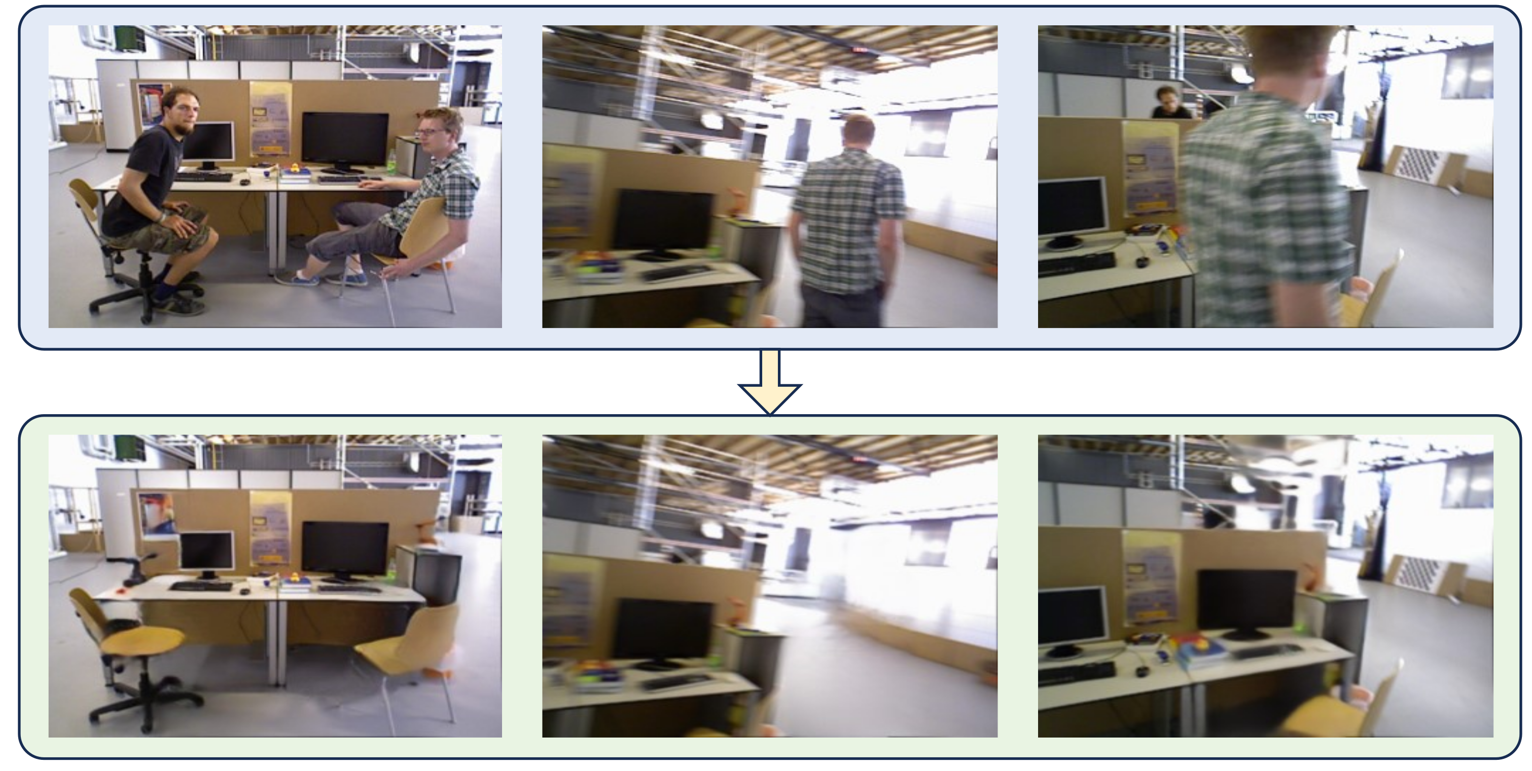
Figure 5: Example of inpainting on the TUM-RGBD dataset.

4 Experiments & Analyisis

We use sequences from both the TUM-RGBD [49] and the recently released GRADE [8] datasets in our evaluations. TUM-RGBD is a set of indoor video RGBD sequences widely adopted in the evaluations of most dynamic SLAM approaches. Specifically, we use the four fr3/walking dynamic sequences {halfsphere, static, rpy, xyz}. Each one of those has a duration of 35.81, 24.83, 30.61, and 28.83 seconds respectively. From GRADE we use all the D, DH, WO, WOH, S, SH, F, FH experiments. We selected them because they represent synthetic sequences for dynamic SLAM which proved to be challenging for many dynamic SLAM methods [9]. The duration of each one of those sequences is 60 seconds. S[H] represents experiments recorded in static environments, D[H] in environments with moving people, F[H] have additional randomly flying objects and WO[H] sequences with occlusions of the camera sensor. The H indicates experiments in which the camera is forced to be kept horizontal, rather than freely moving. More details can be found in the GRADE paper [8]. Additional processing is necessary on the TUM-RGBD data to obtain the static background images. For that we use E2FGVI [30] video inpainting. We adjust the input frames strategy of E2FGVI with a 50-frames sliding window approach with 100 frames bootstrap to overcome the high GPU usage of the method. We then extract the reference frames based on the closest covisible ones using ground-truth poses, rather than the original selection based on time intervals. An example of the inpainted frames is provided in Fig. 5. The GRADE’s framework instead provides a way to re-render images captured in dynamic scenes without the dynamic objects through their experiment repetition tool. By doing so, we obtained a frame-by-frame correspondence of background images. In our experiments, for both the inpainting and the splatting view synthesis, we use the ground truth pose of the camera for the necessary transformations. While this is a limiting factor of the current proposed approach, note that a neighboring frame-by-frame pose variation can be estimated or optimized through different VO, VIO, DNN or other modules with good approximations.

For our tests we use DynaPix, which includes all the edits explained in Sec. 3, and compare results against ORB-SLAM2, its underlying SLAM framework. Moreover, we also introduce DynaPix-D, which combines DynaPix with DynaSLAM [3], a popular state-of-the-art dynamic SLAM approach. While DynaSLAM combines Mask-RCNN to mask pre-defined dynamic classes and ORB-SLAM2 as its backend, DynaPix-D modifies the map point selection based on those same mask filtering. However, we maintain the same strategies on weighted BA in both tracking and backend modules as DynaPix. We utilize the widely accepted RMSE of absolute trajectory error (ATE) to evaluate pose estimation accuracy. Then, to evaluate the system robustness and similar to the previous work [7, 55, 8, 12], we adopt the tracking rate (TR). This metric, which is often overlooked, represents the ratio between the actually tracked time over the entire sequence duration.

Our results on the GRADE dataset are reported in Tab. 1 and Tab. 2, while the ones for the TUM-RGBD sequences are in Tab. 3. For each combination of sequence and method we perform ten experiment runs and report the mean and standard deviation on both metrics, as well as the overall averages. We use the static sequences of GRADE to show that our DynaPix does not degrade the performance of the used SLAM framework in those situations and to further compare the improvements between static and dynamic scenes.

		STATIC SEQUENCE				DYNAMIC SEQUENCE
		DynaPix		ORB-SLAM2		DynaPix		ORB-SLAM2
		ATE [m]	TR	ATE [m]	TR	ATE [m]	TR	ATE [m]	TR
FH	mean	0.006	1.00	0.010	1.00	0.035	1.00	0.248	1.00
	std	0.000	0.00	0.002	0.00	0.016	0.00	0.103	0.00
F	mean	0.230	0.86	0.330	0.90	0.291	0.20	0.359	0.35
	std	0.426	0.00	0.507	0.01	0.108	0.01	0.156	0.03
DH	mean	0.005	0.18	0.005	0.18	0.006	0.18	0.005	0.18
	std	0.001	0.00	0.001	0.01	0.006	0.00	0.001	0.01
D	mean	0.023	0.98	0.018	0.97	0.032	0.98	0.317	0.99
	std	0.006	0.01	0.002	0.03	0.010	0.02	0.043	0.01
WOH	mean	0.012	0.54	0.013	0.54	0.009	0.54	0.016	0.54
	std	0.008	0.00	0.010	0.00	0.001	0.00	0.008	0.00
WO	mean	0.040	0.44	0.038	0.83	0.023	0.20	0.168	0.20
	std	0.023	0.35	0.021	0.32	0.002	0.00	0.022	0.00
SH	mean	0.010	1.00	0.012	1.00	-	-	-	-
	std	0.001	0.00	0.002	0.00	-	-	-	-
S	mean	0.010	1.00	0.011	1.00	-	-	-	-
	std	0.001	0.00	0.001	0.00	-	-	-	-
Average		0.042	0.75	0.055	0.80	0.066	0.52	0.185	0.54

Table 1: ATE RMSE [m] and Tracking Rate (TR) Results of DynaPix and ORB-SLAM2 on GRADE Dataset.

Starting from the synthetic data, we can see that, in general, the experiments performed better on the static version of each sequence with respect to the corresponding dynamic ones. This was expected and holds for all methods. We can already see how using the TR alongside the ATE is essential to analyze these results. Taking the F experiment in Tab. 1 as an example we can see that, while the ATE is similar to the ORB-SLAM2, the TR is 90% for the static sequence but only 35% on the dynamic one. We can also notice that DynaPix does not adversely affect the performance of the original ORB-SLAM2 when performing SLAM on static experiments, with the exception of the WO experiments in which the TR of DynaPix is almost half of the one with ORB-SLAM2 (see Sup). However, the standard variations on these experiments indicate how unsure these two particular results are in both ATE and TR metrics. Considering DynaPix-D and DynaSLAM results on the static sequences, we observe that our approach has better results on both TR and ATE in various experiments like F, DH, D, WO, as well as $10\%$ on the average ATE and $\sim 4\%$ on average TR.

		STATIC SEQUENCE				DYNAMIC SEQUENCE
		DynaPix-D		DynaSLAM		DynaPix-D		DynaSLAM
		ATE [m]	TR	ATE [m]	TR	ATE [m]	TR	ATE [m]	TR
FH	mean	0.007	1.00	0.012	1.00	0.023	1.00	0.232	0.98
	std	0.000	0.00	0.005	0.00	0.006	0.00	0.041	0.02
F	mean	0.325	0.88	0.529	0.82	0.571	0.37	0.864	0.42
	std	0.498	0.01	0.526	0.04	0.265	0.20	0.217	0.07
DH	mean	0.004	0.18	0.013	0.07	0.010	0.14	0.011	0.10
	std	0.001	0.00	0.009	0.03	0.011	0.04	0.003	0.02
D	mean	0.019	0.98	0.024	0.98	0.041	0.96	0.050	0.89
	std	0.004	0.02	0.008	0.02	0.026	0.03	0.009	0.05
WOH	mean	0.011	0.54	0.015	0.54	0.010	0.54	0.012	0.54
	std	0.013	0.00	0.017	0.00	0.004	0.00	0.002	0.00
WO	mean	0.206	0.87	0.043	0.78	0.641	0.20	0.083	0.08
	std	0.399	0.21	0.022	0.28	0.386	0.00	0.010	0.00
SH	mean	0.012	1.00	0.010	1.00	-	-	-	-
	std	0.003	0.00	0.001	0.00	-	-	-	-
S	mean	0.009	1.00	0.010	1.00	-	-	-	-
	std	0.001	0.00	0.002	0.00	-	-	-	-
Average		0.074	0.81	0.082	0.78	0.216	0.54	0.209	0.50

Table 2: ATE RMSE [m] and Tracking Rate (TR) Results of DynaPix-D and DynaSLAM on GRADE Dataset.

Considering now the experiments run on data with dynamic entities, DynaPix and DynaPix-D consistently overcome the corresponding methods with considerable margins. The TR of WO with DynaPix-D, for example, is 2.5 times better than DynaSLAM, although with a far worse ATE linked to the longer tracking time. The ATE of the same sequence obtained by DynaPix is only $\sim 13\%$ than the original one obtained through ORB-SLAM2, but with the same TR. An exception to that is the F sequence on both DynaPix and DynaPix-D, which have respectively 15% and 5% shorter tracking times. This experiment has the camera facing a featureless wall, which can make the SLAM backend stop working on some runs since no recovery procedure is devised for such situations. Despite this, DynaPix performs 3 times better than ORB-SLAM2 in ATE with similar tracking rates despite the 15% drop on the F experiment. On the other hand, DynaPix-D shows a 10% relative TR improvement with respect to DynaSLAM with a marginally worse ATE of 2 cm, despite the significantly worse ATE on the WO sequence of about 60 cm. It is interesting to notice how the dynamics of the WOH sequence seem not to affect the results, given that the metrics are close on both the static and dynamic tests. This is probably due to the camera facing a featureless area during the experiment, while ORB-SLAM2 does not provide robust recovery procedures for such situations. Overall, we can see that, on average, DynaPix performs better than DynaPix-D and ORB-SLAM on both static and dynamic sequences, making it the best overall method. This, holds especially if considering that longer tracking times can be linked to higher ATE.

		DynaPix		ORB-SLAM2		DynaPix-D		DynaSLAM
		ATE [m]	TR	ATE [m]	TR	ATE [m]	TR	ATE [m]	TR
w_half	mean	0.030	1.00	0.607	0.79	0.023	1.00	0.029	1.00
	std	0.002	0.00	0.180	0.11	0.001	0.00	0.001	0.00
w_static	mean	0.012	1.00	0.355	1.00	0.007	1.00	0.007	0.98
	std	0.002	0.00	0.121	0.00	0.001	0.00	0.000	0.00
w_rpy	mean	0.043	1.00	0.744	0.99	0.123	0.98	0.040	0.86
	std	0.007	0.00	0.115	0.01	0.107	0.03	0.008	0.032
w_xyz	mean	0.018	1.00	0.732	0.84	0.014	1.00	0.016	0.92
	std	0.002	0.00	0.102	0.11	0.000	0.00	0.001	0.00
Average		0.026	1.00	0.610	0.91	0.041	0.99	0.023	0.94

Table 3: ATE RMSE [m] and Tracking Rate (TR) Results of DynaPix, ORB-SLAM2, DynaPix-D, and DynaSLAM on the TUM-RGBD Walking Sequences.

Having verified that our method performs better with respect to both ORB-SLAM2 and DynaSLAM on the GRADE data, we proceed to analyze the results of our experiments with real data, which are reported in Tab. 3. With a 23 times improvement on the ATE of DynaPix and 100% TR of DynaPix, we perform better than any compared approach. DynaPix[-D] methods bring a consistent TR improvement alongside better ATE. The only variation to that is in the w_rpy experiment, in which the ATE performs on average worse but with a wide standard deviation, indicating that the method is not stable to fast rotations of the camera as desired. This, however, is linked to a $12\%$ higher TR, which can clearly adversely affect the ATE metric. Thus, we can conclude that while on synthetic dynamic sequences we are still limited by occlusions and textureless areas that cause drift and loss of tracking, on real-world ones our method has the best performance overall.

5 Conclusion

In this paper we introduce DynaPix, a novel dynamic SLAM method based on pixel-wise motion probability and an optimized ORB-SLAM2 framework. We introduced a novel two-staged approach to compute per-pixel motion probabilities by blending movable and moving estimations obtained respectively through static/dynamic frame differencing and static/dynamic splatted optical flow subtraction. The motion probabilities are then used in the ORB-SLAM2 framework within a new mechanism to filter map points while retaining probability during tracking and backend optimization procedures. Our extensive testing with both real and synthetic data shows not only that using tracking rates to analyze SLAM results is of fundamental importance but also that DynaPix performs consistently better than ORB-SLAM2 and DynaSLAM. To address the current limitations of this approach, future works include making use of estimated camera poses in the motion probability estimation pipeline and better recovery procedures to address the low tracking rate we observed on synthetic data.

Supplementary Material

A Overview

In this supplementary material, we present additional information about both our approach and our experimental analysis. In Sec. B we detail our modifications to the E2FGVI framework with examples of inpainted frames on TUM-RGBD dataset. In Sec. C we show the complete workflow with explanatory images of both the movable and moving probability synthesis as well as additional visualization examples of our method. Finally, in Sec. D, we report all our extended results and some additional box plots based on the tracking rate.

B Inpainting of TUM-RGBD Dataset

As mentioned in Sec. 4, the static background images are essential for our implementation. Those are not directly available for the TUM-RGBD sequences. We use the end-to-end flow-guided video inpainting (E2FGVI) technique to eliminate dynamic objects. With an NVIDIA Quadro P5000 with 16 GB of memory, E2FGVI can only load a limited number of frames. To overcome this limitation for longer sequences, we adopt a 50-frame sliding window approach with 100 frames bootstrap. In this way, the inpainting module can process 50 new frames with 50 initially inpainted frames from the last step. The initially inpainted frames can also be adjusted during the new processing cycle, which can be formulated as:

$$\begin{split}I^{i}_{inpaint}(x,y)&=\lambda\cdot I^{i}_{init}(x,y)+(1-\lambda)\cdot I^{i}_{new}(x,y)\\ \end{split}$$ (12)

where $\lambda=0.5$ in our deployment. Despite the original framework has remarkable performance on static/slightly moving camera views, it is difficult to adapt to varying environments with long-term moving cameras. The original framework takes use of neighboring frames and reference frames (extracted based on specific time intervals) to inpaint the current frame. In order to further provide sufficient background information in long-term sequences, we modify the selection strategy of the reference frames to remove irrelevant frames that are observing irrelevant areas. Given the ground-truth camera poses, we select the frames with the closest viewpoint as reference frames which should not be overlapped with the neighboring frames. In this way, these new reference frames can largely cover the possible background regions to improve the inpainting process.

As shown in Fig. iii, we show the inpainted frames from various viewpoints in the TUM-RGBD dataset, where our modified E2FGVI can also generalize to blurry images and provide reliable inpainting performance in different camera angles. We also exhibit some failure cases in Fig. i, the main reason lies in that neighboring/reference frames at other timestamps providing false information, such as the objects (e.g. chairs, books) actually staying at other positions in the current frame. Another reason lies in the fact that reference frames sometimes can not provide sufficient information about the occluded background, leading to a large blur in some cases.

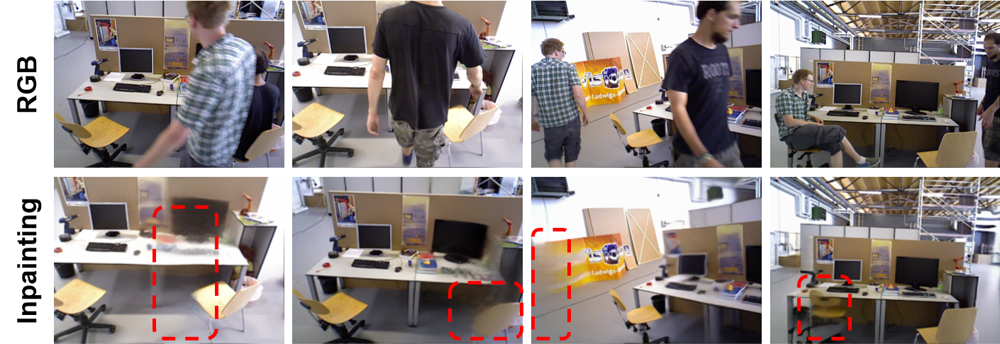
Figure i: Visualization of failure cases of inpainting process.

C Motion Probability Demonstrations

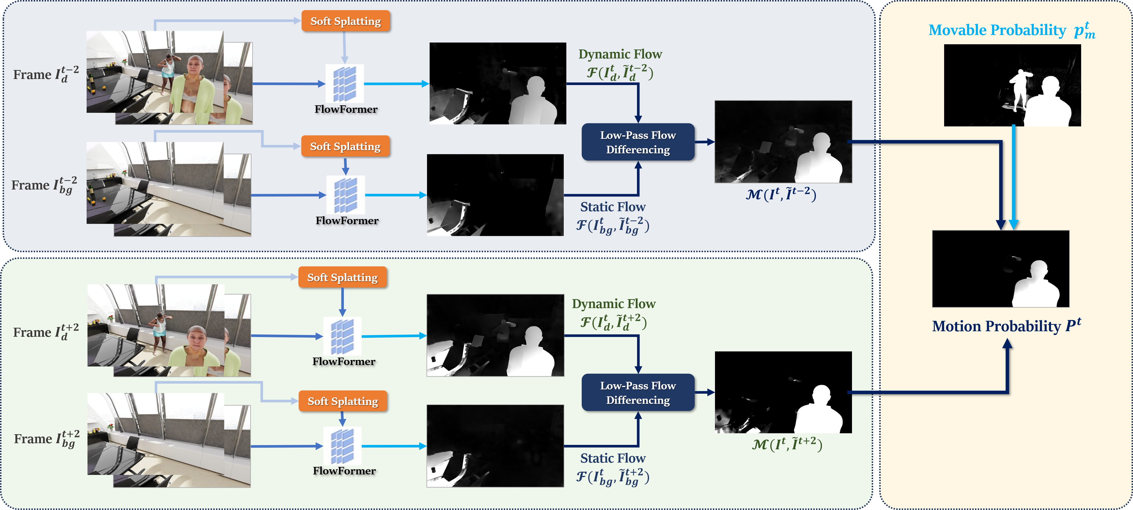
Figure ii: Flow diagram of moving estimation (Sec. 3.1.2) and final motion probability (Sec. 3.1.3).

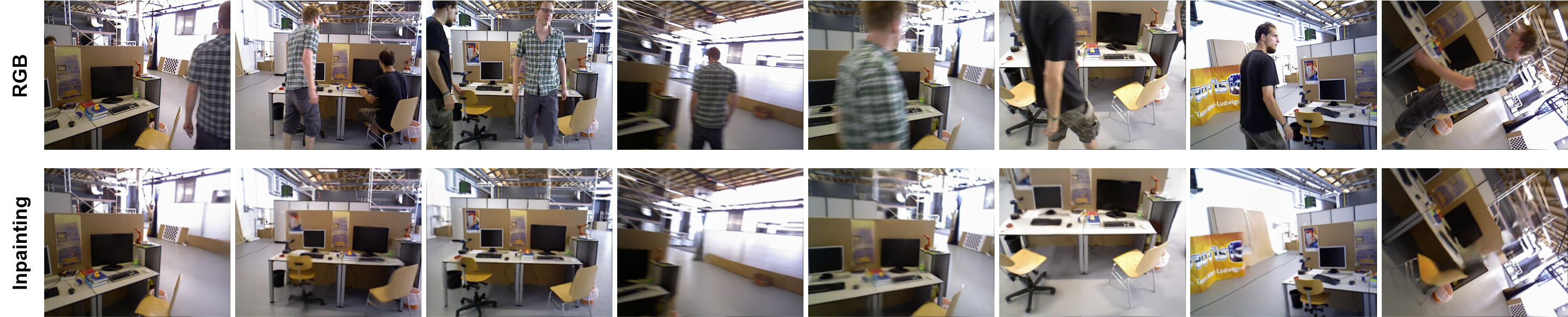
Figure iii: Visualization of inpainted background images from TUM-RGBD dataset, covering blurry images and various viewpoints.

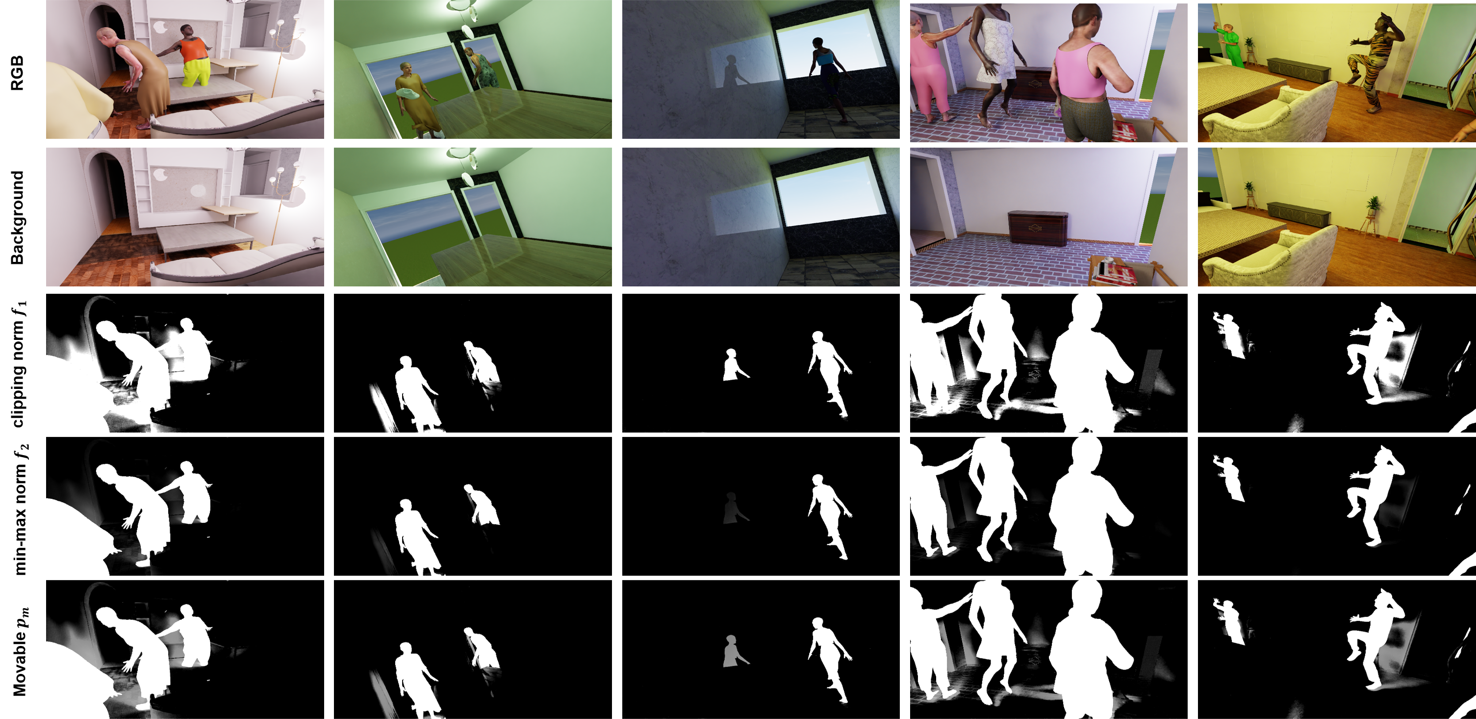
Figure iv: Visualization of movable region estimation, covering shadows, reflections, and movable objects.

In this section, we demonstrate the progressive improvements of our two-staged probability estimation module as shown in Fig.ii. In terms of the movable estimation part, the combination of $f_{1}$ and $f_{2}$ in Eq. 3 addresses a trade-off on reducing the noisy difference value and capturing the shadow/reflection areas. More illustrations for this process are exhibited in Fig. iv. The movable distribution acts as a confidence score to further constrain the following moving estimation to effectively eliminates the inherent errors on the static regions (see Fig. vi).

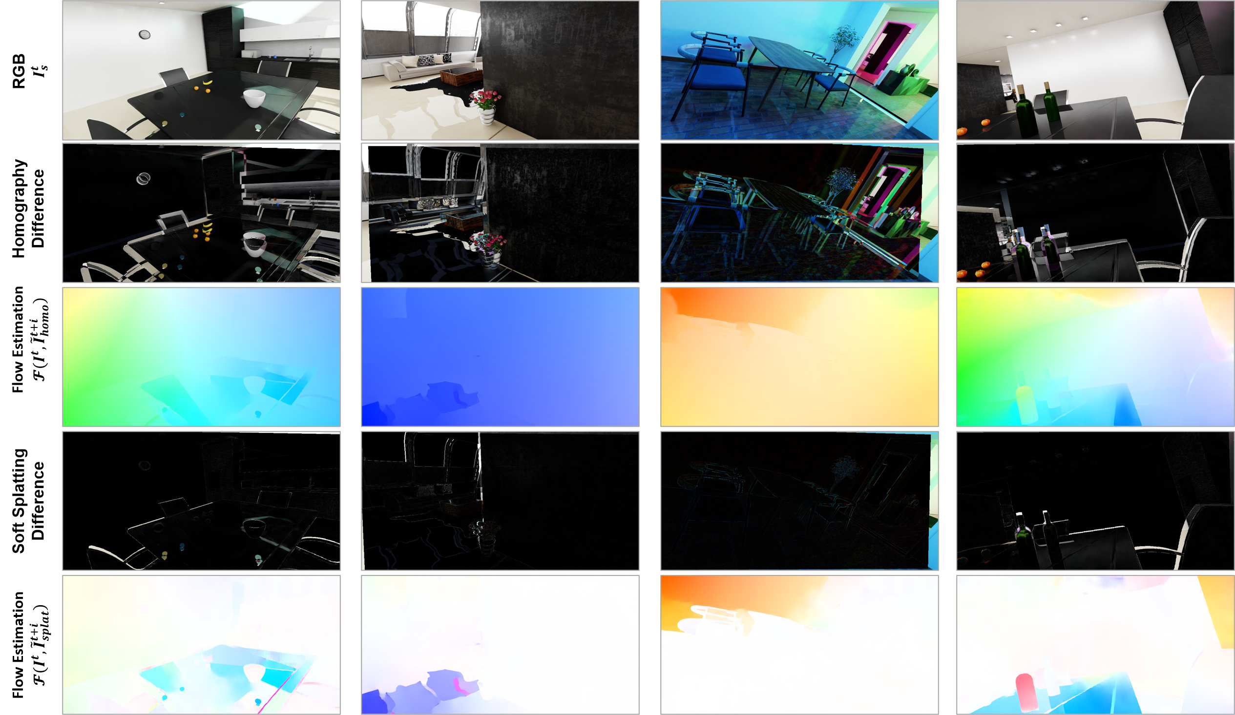
Figure v: Visualization of the performance of projecting frames through Soft Splatting or Homography Transformation techniques using frames for static scenes. The second line and fourth line differences the frame $\widetilde{I}^{t+i}$ and $I^{t}$ to illustrate the alignment performance across the frames, while the third line and fifth line demonstrate their effects in flow estimation $\mathcal{F}({I}^{t},\widetilde{I}^{t+i})$, where flow magnitude should ideally approach to 0 in static regions as discussed in Eq. 5.

As we discussed in Sec. 3.1.2, the view synthesis based on soft-splatting [39] can effectively reduce the aligning error between the reprojected frame $\widetilde{I}^{t+i}$ and current frame ${I}^{t}$, significantly decreasing the errors in flow estimation generated from incomplete elimination of camera motion. In Fig. v we can see the computation of the optical flow on splatted frames gives us a more effective elimination of camera motion than the homography-based method. This is indicated by the coloring of the frame which goes towards white in static regions. Moreover, we can see that there exist similarities between flows estimated on static and dynamic scenes, as shown in details in Fig. vi. Given this insight, we developed a flow differencing approach to further eliminate residual camera motion. This can decrease the flow estimation error on the common static regions, while the low-pass filter stores the original estimation result in dynamic regions to avoid false subtraction.

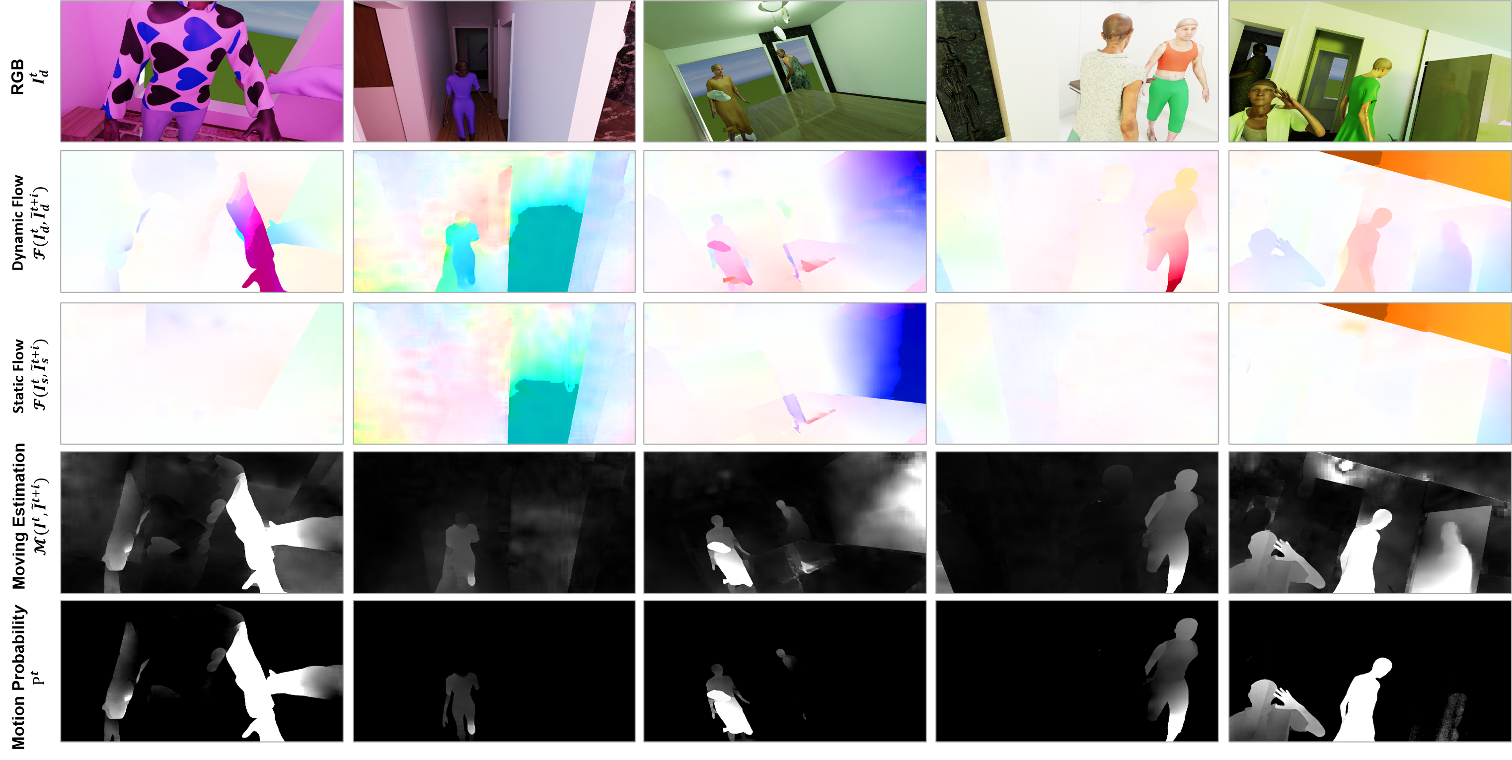
Figure vi: Visualization of the moving estimation and final motion probability. The second line and third line represent the flow estimated on dynamic scenes $\mathcal{F}({I}_{d}^{t},\widetilde{I}_{d}^{t+i})$ and static scenes $\mathcal{F}({I}_{s}^{t},\widetilde{I}_{s}^{t+i})$ respectively, exhibiting similar estimation errors in common static regions. The fourth line demonstrates the moving estimation $\mathcal{M}({I}^{t},\widetilde{I}^{t+i})$ through flow differencing. The fifth line denotes the blended motion probability $P^{t}$ by multiplying movable probability $p_{m}^{t}$

We also exhibit some failure cases in Fig. vii, which mainly result from the false correspondences in textureless regions (e.g. wall, floor). The specific reason lies in that underlying flow estimation networks fail to capture the correct pixel correspondences in these regions, leading to false moving estimation $\mathcal{M}({I}^{t},\widetilde{I}^{t+i})$ on the static regions. Despite many of these can be constrained by multiplying them with movable probability, this module sometimes fails to provide accurate motion estimation when there is occlusion. The occlusion directly influences the background differencing process and falsely classifies many regions as movable, being incapable of further reducing the errors generated from flow estimation.

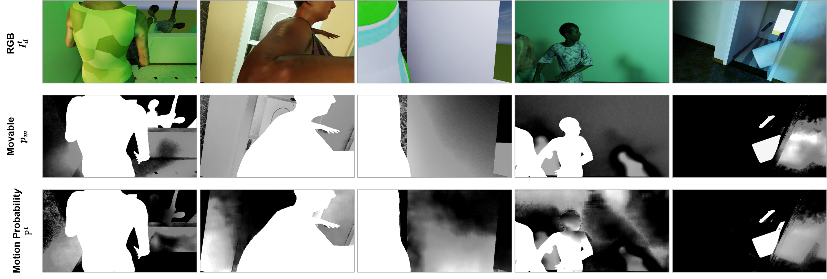
Figure vii: Visualization of failure cases on motion probability.

D Detailed SLAM Evaluation Experiments

In Sec. 4, we exhibit the necessary experimental results to demonstrate our effectiveness in both synthetic sequences and real-world sequences, followed by the analysis by comparing performance in static/dynamic scenes. Here, we first report the detailed experimental result of each one of the ten runs for each sequence. Then, we analyze the distribution of such results using box plots based on tracking rate amounts to provide more insights into these results.

The detailed results help us put in perspective what we expressed in the paper. For example, we can see how in both sequences F and WO there are wide variations in the outputs of both the tracking rate and ATE, both for the static and dynamic case. This indicates that in those sequences there are critical points which make the method fail in some situations based on the stochastic nature of the underlying SLAM frameworks. These failures are mostly linked to featureless areas, that make the method lose track of the camera movement, and the absence of a subsequent strong recovery procedure. We can also see how in the tracking rates there is little variability in most situations for both our and the benchmark methods.

Although the average value of both absolute trajectory error (ATE) and tracking rate (TR), with the corresponding standard deviations, can provide an overall evaluation of various methods, comparing the ATE with various TR is also necessary to gather insights on the relations between these two. For this reason we provide a series of plots, one for each experiment, in which, given a tracking rate interval, we report the corresponding ATE statistics for the four methods. We defined four non-overlapping TR intervals, which are high ($\geq 0.95$), middle ($\geq 0.85$), low ($\geq 0.70$), and rare ($\leq 0.70$) tracking rate. Ideally, the estimation distribution should lie in the left-bottom corner, i.e. low trajectory error and high tracking rate, without any presence in other sectors. Anyway, given a sector, the lower the ATE the better. From these plots we can see how DynaPix and DynaPix-D are often located in that region. Notably, with the exception of the WO - Static Scene experiment, both are always located in the left-most populated box with better performance than the corresponding method both in terms of ATE and variance of the results, making them not only better but stabler. This holds true for both the synthetic and real-world datasets and especially, but not only, in FH, WOH, S, D, DH, halfsphere, static and rpy sequences. Moreover, these plots also evidence the fact that DynaSLAM is often located alone in the right-most section, indicating poor tracking rates in almost all synthetic experiments and in both the halfsphere and rpy TUM-RGBD sequences. This is clearly reflected by DynaPix-D and evidence of the influence of semantic masks and how blindly discarding features because belonging to a potentially dynamic object can worsen the performance of the method.

	DYNAMIC SEQUENCE								STATIC SEQUENCE
	DynaPix		ORB-SLAM2		DynaPix-D		DynaSLAM		DynaPix		ORB-SLAM2		DynaPix-D		DynaSLAM
	ATE [m]	TR	ATE [m]	TR	ATE [m]	TR	ATE [m]	TR	ATE [m]	TR	ATE [m]	TR	ATE [m]	TR	ATE [m]	TR
F	0.312	0.19	0.443	0.33	0.520	0.31	1.006	0.49	0.010	0.86	1.066	0.90	0.058	0.89	0.059	0.85
	0.237	0.20	0.494	0.35	0.931	0.65	0.896	0.33	1.035	0.86	0.014	0.89	1.053	0.89	0.009	0.81
	0.205	0.20	0.230	0.28	0.599	0.21	0.895	0.42	0.059	0.86	0.013	0.90	0.009	0.87	1.028	0.85
	0.580	0.21	0.344	0.35	0.936	0.65	0.920	0.44	0.008	0.87	0.012	0.91	0.009	0.89	0.059	0.86
	0.207	0.20	0.413	0.35	0.352	0.31	1.012	0.53	1.039	0.86	0.010	0.91	1.031	0.86	0.012	0.75
	0.288	0.20	0.461	0.36	0.363	0.32	0.908	0.43	0.058	0.86	1.064	0.90	0.008	0.89	1.032	0.84
	0.265	0.20	0.083	0.39	0.937	0.64	0.914	0.40	0.058	0.86	0.012	0.91	0.008	0.89	1.023	0.85
	0.243	0.19	0.140	0.37	0.332	0.19	0.917	0.45	0.009	0.86	1.065	0.90	1.053	0.89	1.030	0.85
	0.309	0.23	0.537	0.34	0.342	0.19	0.910	0.44	0.009	0.86	0.015	0.91	0.009	0.89	1.028	0.85
	0.266	0.20	0.444	0.37	0.397	0.22	0.257	0.28	0.010	0.85	0.025	0.91	0.011	0.86	0.015	0.74
MEAN	0.291	0.20	0.359	0.35	0.571	0.37	0.864	0.42	0.230	0.86	0.330	0.90	0.325	0.88	0.529	0.82
STD	0.108	0.01	0.156	0.03	0.265	0.20	0.217	0.07	0.426	0.00	0.507	0.01	0.498	0.01	0.526	0.04

Table i: All the 10 runs ATE and TR results of all four methods on the GRADE F sequence both in its static and dynamic version.

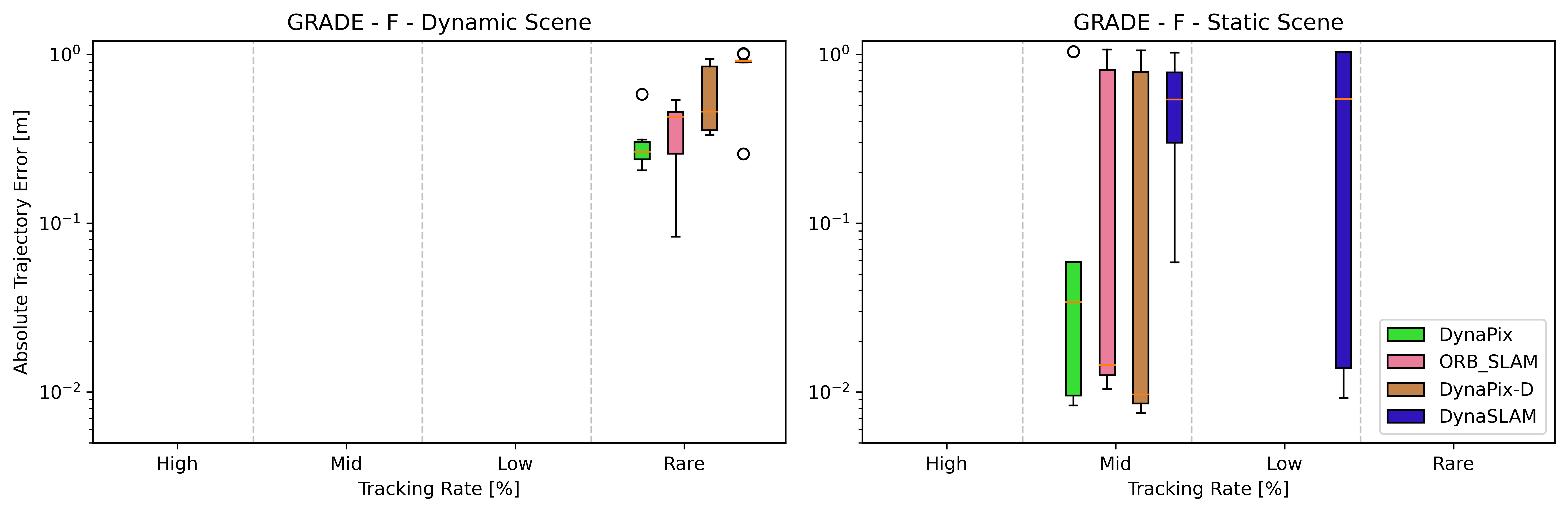
Figure viii: Box-Plot of results of the four methods tested on the F static and dynamic sequences using the tracking rate buckets and the ATE results.

	DYNAMIC SEQUENCE								STATIC SEQUENCE
	DynaPix		ORB-SLAM2		DynaPix-D		DynaSLAM		DynaPix		ORB-SLAM2		DynaPix-D		DynaSLAM
	ATE [m]	TR	ATE [m]	TR	ATE [m]	TR	ATE [m]	TR	ATE [m]	TR	ATE [m]	TR	ATE [m]	TR	ATE [m]	TR
FH	0.036	1.00	0.251	1.00	0.021	1.00	0.240	1.00	0.007	1.00	0.009	1.00	0.007	1.00	0.008	1.00
	0.027	1.00	0.246	1.00	0.021	1.00	0.215	0.99	0.007	1.00	0.009	1.00	0.007	1.00	0.008	1.00
	0.023	1.00	0.249	1.00	0.024	1.00	0.215	0.99	0.006	1.00	0.011	1.00	0.007	1.00	0.020	1.00
	0.062	1.00	0.401	1.00	0.034	1.00	0.336	0.98	0.007	1.00	0.010	1.00	0.007	1.00	0.023	1.00
	0.049	1.00	0.143	1.00	0.018	1.00	0.191	0.95	0.007	1.00	0.007	1.00	0.007	1.00	0.009	1.00
	0.020	1.00	0.097	1.00	0.018	1.00	0.224	0.94	0.006	1.00	0.008	1.00	0.007	1.00	0.010	1.00
	0.048	1.00	0.125	1.00	0.030	1.00	0.239	0.94	0.007	1.00	0.009	1.00	0.007	1.00	0.009	1.00
	0.018	1.00	0.253	1.00	0.029	1.00	0.250	0.99	0.007	1.00	0.011	1.00	0.007	1.00	0.014	1.00
	0.050	1.00	0.360	1.00	0.016	1.00	0.194	1.00	0.007	1.00	0.013	1.00	0.007	1.00	0.012	1.00
	0.019	1.00	0.352	1.00	0.016	1.00	0.219	0.99	0.006	1.00	0.012	1.00	0.007	1.00	0.010	1.00
MEAN	0.035	1.00	0.248	1.00	0.023	1.00	0.232	0.98	0.006	1.00	0.010	1.00	0.007	1.00	0.012	1.00
STD	0.016	0.00	0.103	0.00	0.006	0.00	0.041	0.02	0.000	0.00	0.002	0.00	0.000	0.00	0.005	0.00

Table ii: All the 10 runs ATE and TR results of all four methods on the GRADE FH sequence both in its static and dynamic version.

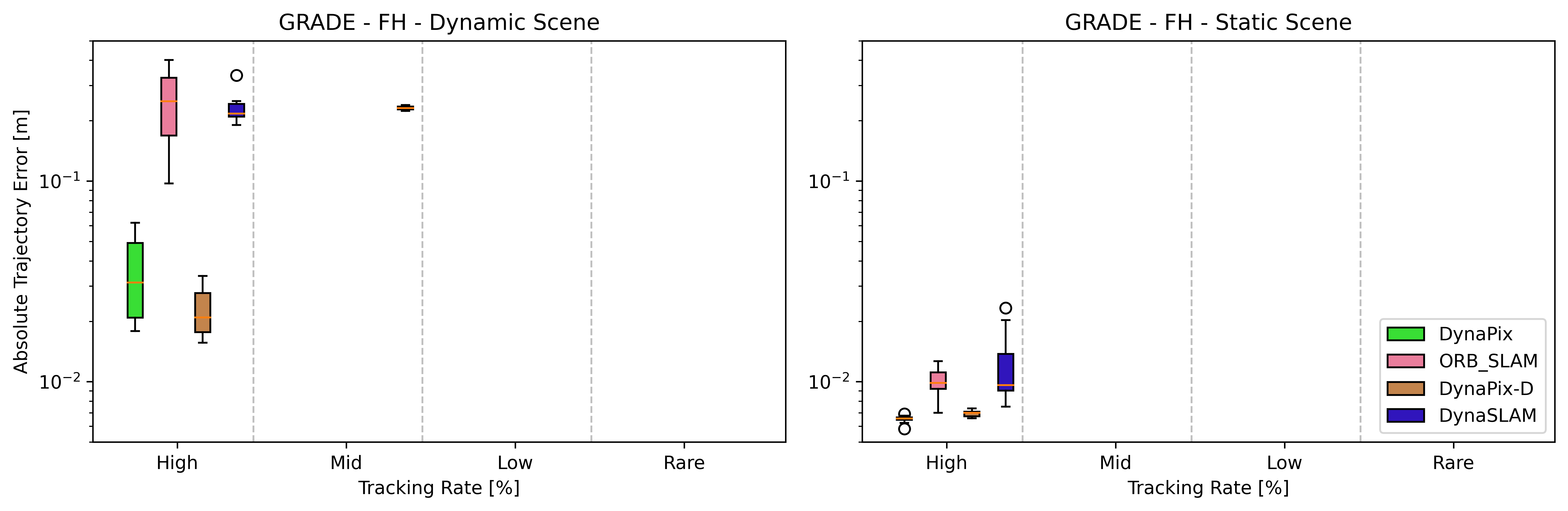
Figure ix: Box-Plot of results of the four methods tested on the FH static and dynamic sequences using the tracking rate buckets and the ATE results.

	DYNAMIC SEQUENCE								STATIC SEQUENCE
	DynaPix		ORB-SLAM2		DynaPix-D		DynaSLAM		DynaPix		ORB-SLAM2		DynaPix-D		DynaSLAM
	ATE [m]	TR	ATE [m]	TR	ATE [m]	TR	ATE [m]	TR	ATE [m]	TR	ATE [m]	TR	ATE [m]	TR	ATE [m]	TR
D	0.017	1.00	0.263	0.99	0.018	0.99	0.052	0.83	0.022	0.99	0.020	1.00	0.015	0.99	0.016	0.97
	0.042	0.99	0.335	0.99	0.023	0.99	0.061	0.95	0.018	0.99	0.019	0.93	0.017	0.95	0.026	0.99
	0.033	0.99	0.312	0.97	0.086	0.96	0.046	0.93	0.021	0.99	0.015	0.99	0.027	0.99	0.026	0.99
	0.051	1.00	0.341	0.99	0.067	0.93	0.049	0.93	0.021	0.99	0.022	0.99	0.023	0.93	0.025	0.99
	0.027	0.99	0.258	0.99	0.018	0.93	0.045	0.86	0.024	0.99	0.022	0.99	0.018	0.99	0.039	0.99
	0.031	0.99	0.407	0.99	0.071	0.93	0.052	0.94	0.020	0.99	0.018	0.92	0.014	0.99	0.018	0.99
	0.041	0.99	0.340	0.99	0.048	0.93	0.056	0.86	0.039	0.99	0.016	0.99	0.017	0.99	0.016	0.93
	0.029	0.99	0.287	0.99	0.017	0.99	0.044	0.83	0.021	0.99	0.020	0.99	0.022	0.99	0.033	0.99
	0.026	0.99	0.317	0.99	0.050	1.00	0.060	0.84	0.021	0.94	0.016	0.93	0.017	0.99	0.025	0.99
	0.023	0.93	0.314	0.99	0.016	1.00	0.030	0.93	0.023	0.99	0.017	0.99	0.017	0.99	0.018	0.99
MEAN	0.032	0.99	0.317	0.99	0.041	0.96	0.050	0.89	0.023	0.98	0.018	0.97	0.019	0.98	0.024	0.98
STD	0.010	0.02	0.043	0.01	0.026	0.03	0.009	0.05	0.006	0.01	0.002	0.03	0.004	0.02	0.008	0.02

Table iii: All the 10 runs ATE and TR results of all four methods on the GRADE D sequence both in its static and dynamic version.

Figure x: Box-Plot of results of the four methods tested on the D static and dynamic sequences using the tracking rate buckets and the ATE results.

	DYNAMIC SEQUENCE								STATIC SEQUENCE
	DynaPix		ORB-SLAM2		DynaPix-D		DynaSLAM		DynaPix		ORB-SLAM2		DynaPix-D		DynaSLAM
	ATE [m]	TR	ATE [m]	TR	ATE [m]	TR	ATE [m]	TR	ATE [m]	TR	ATE [m]	TR	ATE [m]	TR	ATE [m]	TR
DH	0.005	0.18	0.006	0.17	0.005	0.18	0.013	0.12	0.005	0.18	0.005	0.19	0.003	0.18	0.016	0.05
	0.004	0.17	0.005	0.17	0.032	0.09	0.015	0.09	0.006	0.18	0.005	0.17	0.004	0.18	0.006	0.05
	0.005	0.18	0.003	0.19	0.003	0.17	0.012	0.09	0.003	0.18	0.007	0.18	0.005	0.18	0.017	0.05
	0.004	0.18	0.003	0.18	0.003	0.18	0.006	0.09	0.006	0.18	0.005	0.17	0.005	0.18	0.036	0.14
	0.003	0.18	0.007	0.17	0.027	0.07	0.015	0.13	0.006	0.18	0.005	0.19	0.003	0.18	0.008	0.10
	0.005	0.18	0.004	0.17	0.003	0.17	0.010	0.13	0.004	0.17	0.005	0.17	0.005	0.18	0.009	0.05
	0.005	0.17	0.007	0.17	0.017	0.18	0.007	0.09	0.004	0.17	0.003	0.19	0.005	0.18	0.015	0.05
	0.005	0.18	0.005	0.19	0.005	0.14	0.010	0.09	0.004	0.18	0.005	0.19	0.004	0.18	0.005	0.10
	0.005	0.18	0.004	0.19	0.005	0.12	0.010	0.09	0.005	0.17	0.004	0.17	0.005	0.18	0.012	0.05
	0.024	0.18	0.006	0.17	0.005	0.14	0.011	0.09	0.005	0.18	0.004	0.17	0.004	0.18	0.008	0.09
MEAN	0.006	0.17	0.005	0.18	0.010	0.14	0.011	0.10	0.005	0.18	0.005	0.18	0.004	0.18	0.013	0.07
STD	0.006	0.00	0.001	0.01	0.011	0.04	0.003	0.02	0.001	0.00	0.001	0.01	0.001	0.00	0.009	0.03

Table iv: All the 10 runs ATE and TR results of all four methods on the GRADE DH sequence both in its static and dynamic version.

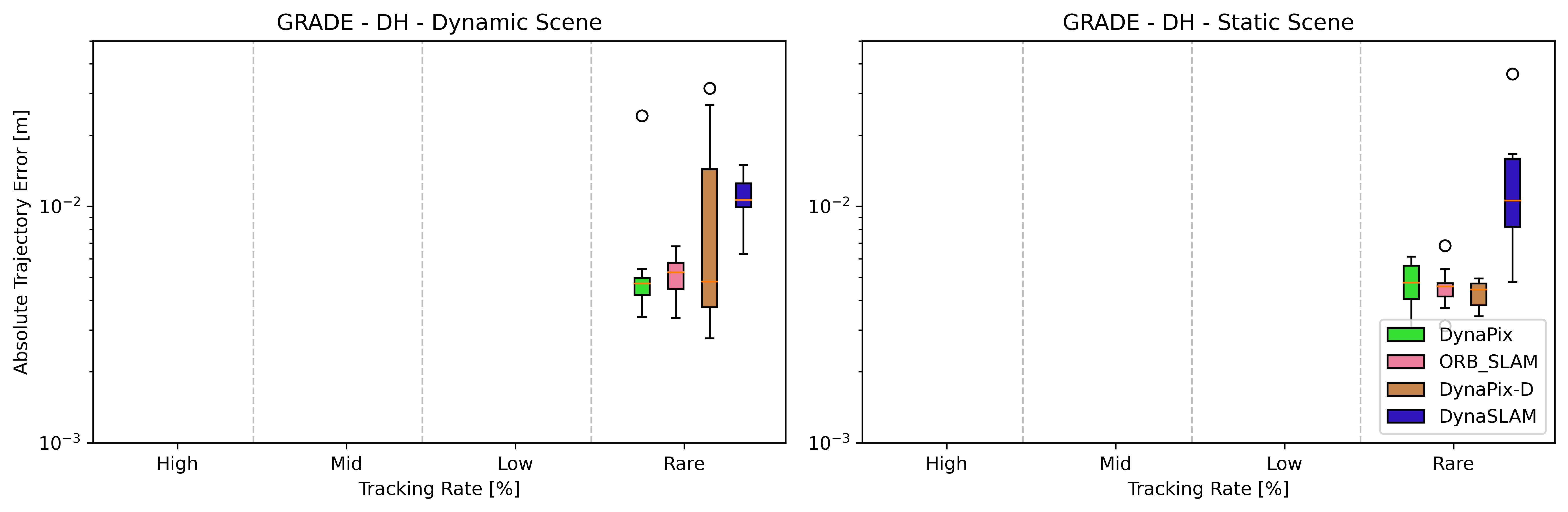
Figure xi: Box-Plot of results of the four methods tested on the DH static and dynamic sequences using the tracking rate buckets and the ATE results.

	DYNAMIC SEQUENCE								STATIC SEQUENCE
	DynaPix		ORB-SLAM2		DynaPix-D		DynaSLAM		DynaPix		ORB-SLAM2		DynaPix-D		DynaSLAM
	ATE [m]	TR	ATE [m]	TR	ATE [m]	TR	ATE [m]	TR	ATE [m]	TR	ATE [m]	TR	ATE [m]	TR	ATE [m]	TR
WO	0.022	0.20	0.152	0.20	0.913	0.20	0.070	0.08	0.022	0.23	0.088	1.00	0.023	0.94	0.039	0.94
	0.028	0.20	0.191	0.20	0.763	0.20	0.092	0.08	0.077	0.94	0.034	0.94	0.032	0.93	0.044	0.33
	0.022	0.20	0.165	0.20	0.826	0.20	0.077	0.08	0.024	0.22	0.024	0.94	0.031	0.94	0.036	0.94
	0.022	0.20	0.222	0.20	1.432	0.20	0.093	0.08	0.018	0.23	0.030	1.00	0.049	0.94	0.092	0.93
	0.023	0.20	0.161	0.20	0.218	0.20	0.083	0.08	0.070	0.22	0.035	0.94	0.431	0.94	0.017	0.22
	0.021	0.20	0.160	0.20	0.208	0.20	0.067	0.08	0.016	0.22	0.024	0.22	0.133	0.26	0.026	0.94
	0.025	0.20	0.150	0.20	0.229	0.20	0.086	0.08	0.020	0.22	0.056	1.00	0.022	0.94	0.046	0.94
	0.023	0.20	0.159	0.20	0.766	0.20	0.089	0.08	0.043	0.22	0.026	1.00	0.018	0.94	0.066	0.93
	0.025	0.20	0.167	0.20	0.444	0.20	0.095	0.08	0.051	0.94	0.017	0.23	1.284	0.93	0.023	0.94
	0.024	0.20	0.154	0.20	0.606	0.20	0.081	0.08	0.054	0.94	0.047	1.00	0.040	0.94	0.046	0.74
MEAN	0.023	0.20	0.168	0.20	0.641	0.20	0.083	0.08	0.040	0.44	0.038	0.83	0.206	0.87	0.043	0.78
STD	0.002	0.00	0.022	0.00	0.386	0.00	0.010	0.00	0.023	0.35	0.021	0.32	0.399	0.21	0.022	0.28

Table v: All the 10 runs ATE and TR results of all four methods on the GRADE WO sequence both in its static and dynamic version.

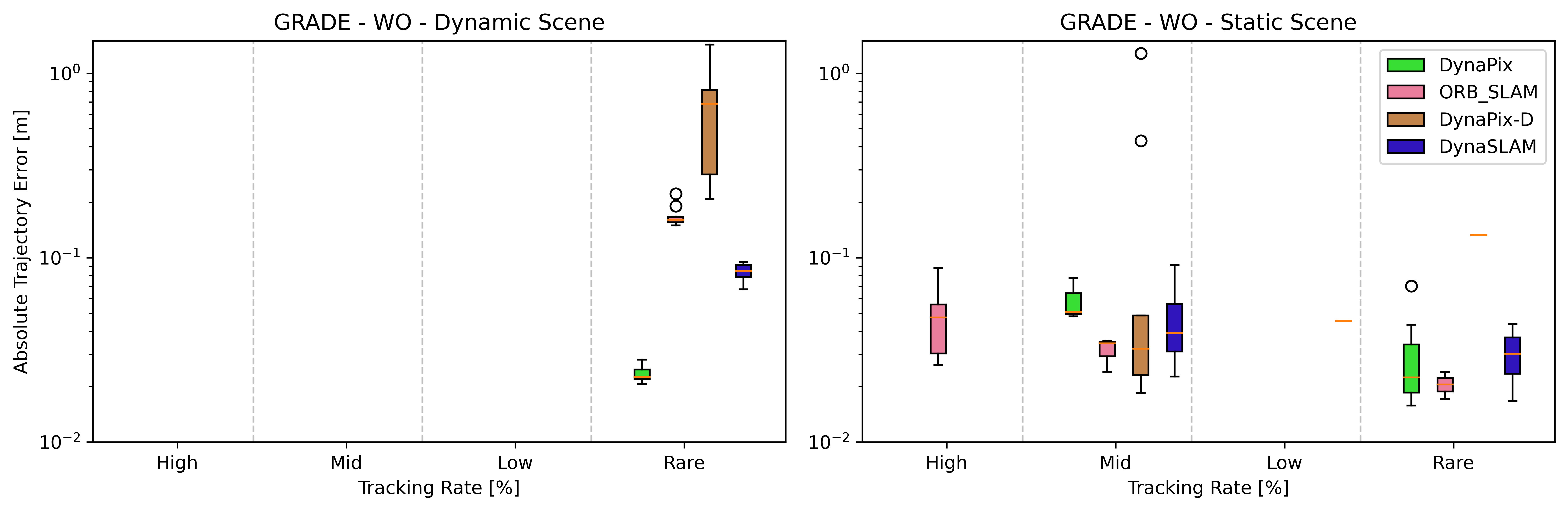
Figure xii: Box-Plot of results of the four methods tested on the WO static and dynamic sequences using the tracking rate buckets and the ATE results.

	DYNAMIC SEQUENCE								STATIC SEQUENCE
	DynaPix		ORB-SLAM2		DynaPix-D		DynaSLAM		DynaPix		ORB-SLAM2		DynaPix-D		DynaSLAM
	ATE [m]	TR	ATE [m]	TR	ATE [m]	TR	ATE [m]	TR	ATE [m]	TR	ATE [m]	TR	ATE [m]	TR	ATE [m]	TR
WOH	0.009	0.54	0.009	0.54	0.009	0.54	0.011	0.54	0.008	0.54	0.040	0.54	0.006	0.54	0.009	0.54
	0.009	0.54	0.022	0.54	0.008	0.54	0.013	0.54	0.031	0.54	0.010	0.54	0.048	0.54	0.009	0.54
	0.009	0.54	0.027	0.54	0.008	0.54	0.011	0.54	0.021	0.54	0.009	0.54	0.007	0.54	0.012	0.54
	0.009	0.54	0.030	0.54	0.009	0.54	0.011	0.54	0.008	0.54	0.015	0.54	0.007	0.54	0.010	0.54
	0.008	0.54	0.010	0.54	0.014	0.54	0.011	0.54	0.007	0.54	0.015	0.54	0.006	0.54	0.010	0.54
	0.008	0.54	0.010	0.54	0.011	0.54	0.014	0.54	0.011	0.54	0.007	0.54	0.007	0.54	0.008	0.54
	0.008	0.54	0.011	0.54	0.019	0.54	0.012	0.54	0.019	0.54	0.007	0.54	0.006	0.54	0.011	0.54
	0.008	0.54	0.012	0.54	0.009	0.54	0.013	0.54	0.007	0.54	0.013	0.54	0.006	0.54	0.009	0.54
	0.010	0.54	0.010	0.54	0.009	0.54	0.016	0.54	0.008	0.54	0.009	0.54	0.005	0.54	0.063	0.54
	0.010	0.54	0.014	0.54	0.008	0.54	0.011	0.54	0.007	0.54	0.009	0.54	0.007	0.54	0.007	0.54
MEAN	0.009	0.54	0.016	0.54	0.010	0.54	0.012	0.54	0.012	0.54	0.013	0.54	0.011	0.54	0.015	0.54
STD	0.001	0.00	0.008	0.00	0.004	0.00	0.002	0.00	0.008	0.00	0.010	0.00	0.013	0.00	0.017	0.00

Table vi: All the 10 runs ATE and TR results of all four methods on the GRADE WOH sequence both in its static and dynamic version.

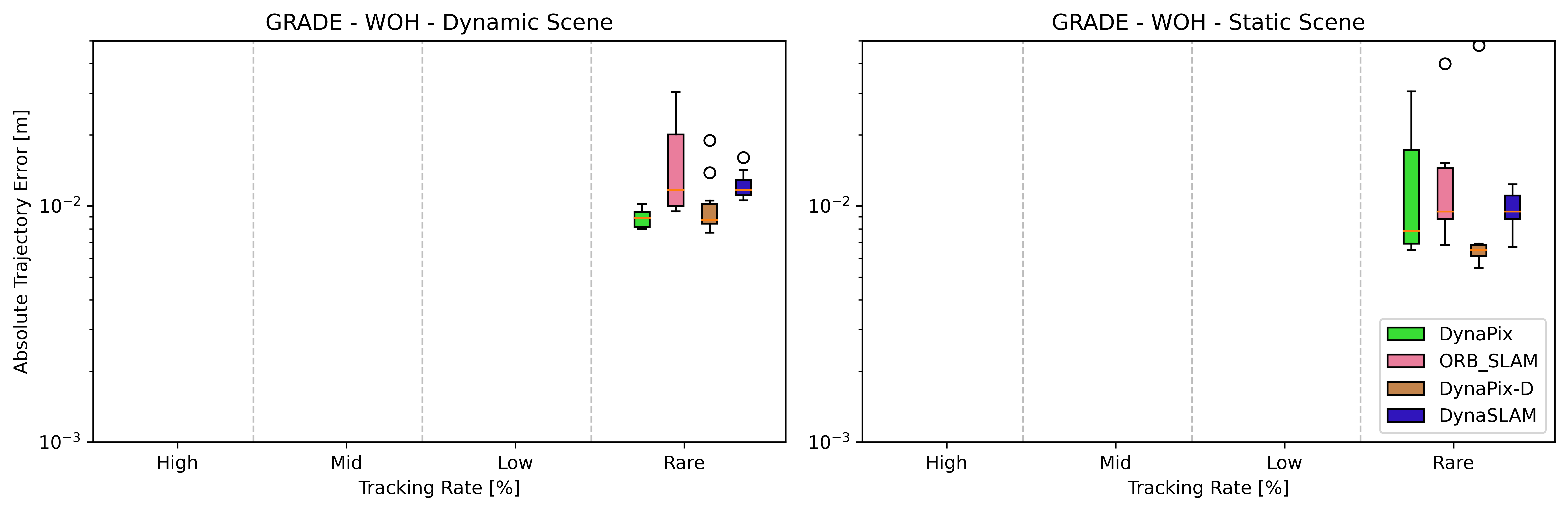
Figure xiii: Box-Plot of results of the four methods tested on the WOH static and dynamic sequences using the tracking rate buckets and the ATE results.

	DynaPix		ORB-SLAM2		DynaPix-D		DynaSLAM
	ATE [m]	TR	ATE [m]	TR	ATE [m]	TR	ATE [m]	TR
S	0.011	1.00	0.011	1.00	0.011	1.00	0.014	1.00
	0.010	1.00	0.009	1.00	0.009	1.00	0.011	1.00
	0.010	1.00	0.010	1.00	0.010	1.00	0.008	1.00
	0.009	1.00	0.010	1.00	0.009	1.00	0.010	1.00
	0.009	1.00	0.011	1.00	0.009	1.00	0.013	1.00
	0.009	1.00	0.012	1.00	0.008	1.00	0.008	1.00
	0.010	1.00	0.012	1.00	0.009	1.00	0.011	1.00
	0.010	1.00	0.012	1.00	0.009	1.00	0.009	1.00
	0.011	1.00	0.011	1.00	0.009	1.00	0.009	1.00
	0.010	1.00	0.010	1.00	0.010	1.00	0.009	1.00
MEAN	0.010	1.00	0.011	1.00	0.009	1.00	0.010	1.00
STD	0.001	0.00	0.001	0.00	0.001	0.00	0.002	0.00

Table vii: All the 10 runs ATE and TR results of all four methods on the GRADE S sequence.

	DynaPix		ORB-SLAM2		DynaPix-D		DynaSLAM
	ATE [m]	TR	ATE [m]	TR	ATE [m]	TR	ATE [m]	TR
SH	0.009	1.00	0.013	1.00	0.009	1.00	0.013	1.00
	0.010	1.00	0.012	1.00	0.016	1.00	0.009	1.00
	0.010	1.00	0.011	1.00	0.012	1.00	0.009	1.00
	0.009	1.00	0.014	1.00	0.015	1.00	0.009	1.00
	0.010	1.00	0.010	1.00	0.008	1.00	0.011	1.00
	0.010	1.00	0.013	1.00	0.010	1.00	0.011	1.00
	0.011	1.00	0.010	1.00	0.016	1.00	0.008	1.00
	0.011	1.00	0.017	1.00	0.012	1.00	0.011	1.00
	0.010	1.00	0.011	1.00	0.010	1.00	0.010	1.00
	0.013	1.00	0.013	1.00	0.009	1.00	0.009	1.00
MEAN	0.010	1.00	0.012	1.00	0.012	1.00	0.010	1.00
STD	0.001	0.00	0.002	0.00	0.003	0.00	0.001	0.00

Table viii: All the 10 runs ATE and TR results of all four methods on the GRADE SH sequence.

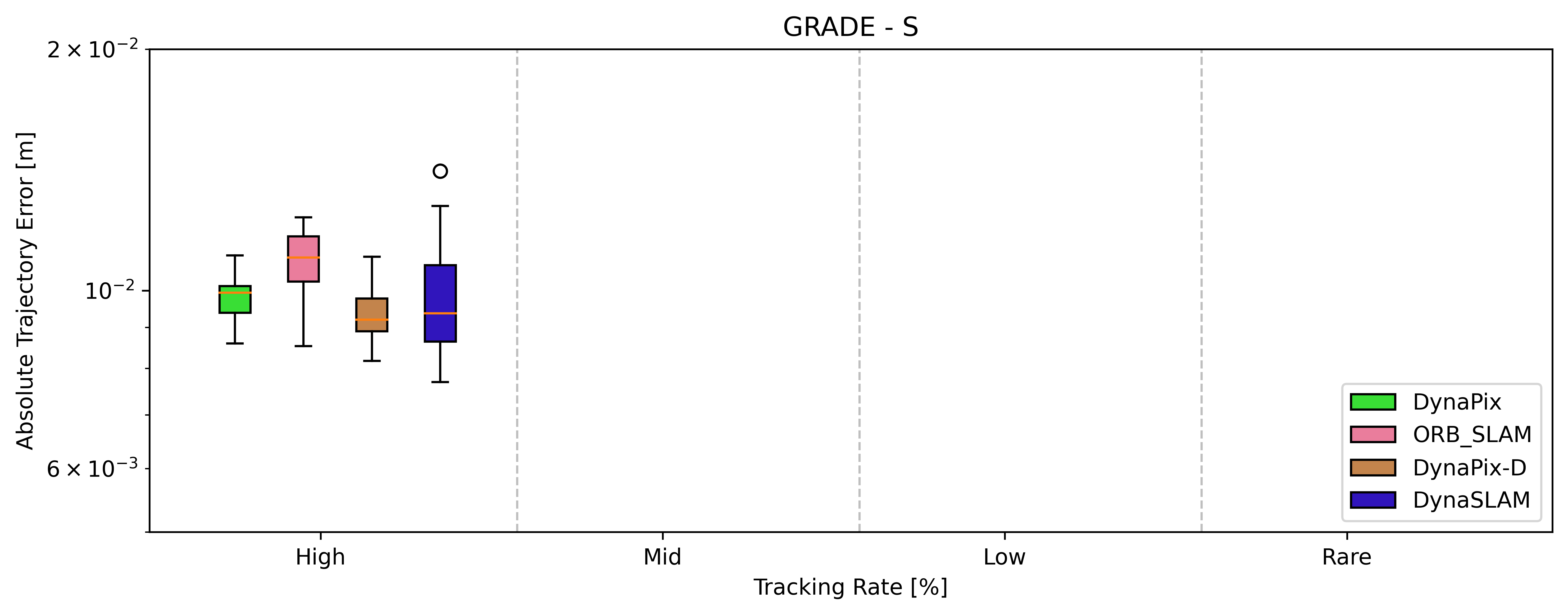
Figure xiv: Box-Plot of results of the four methods tested on the S sequence using the tracking rate buckets and the ATE results.

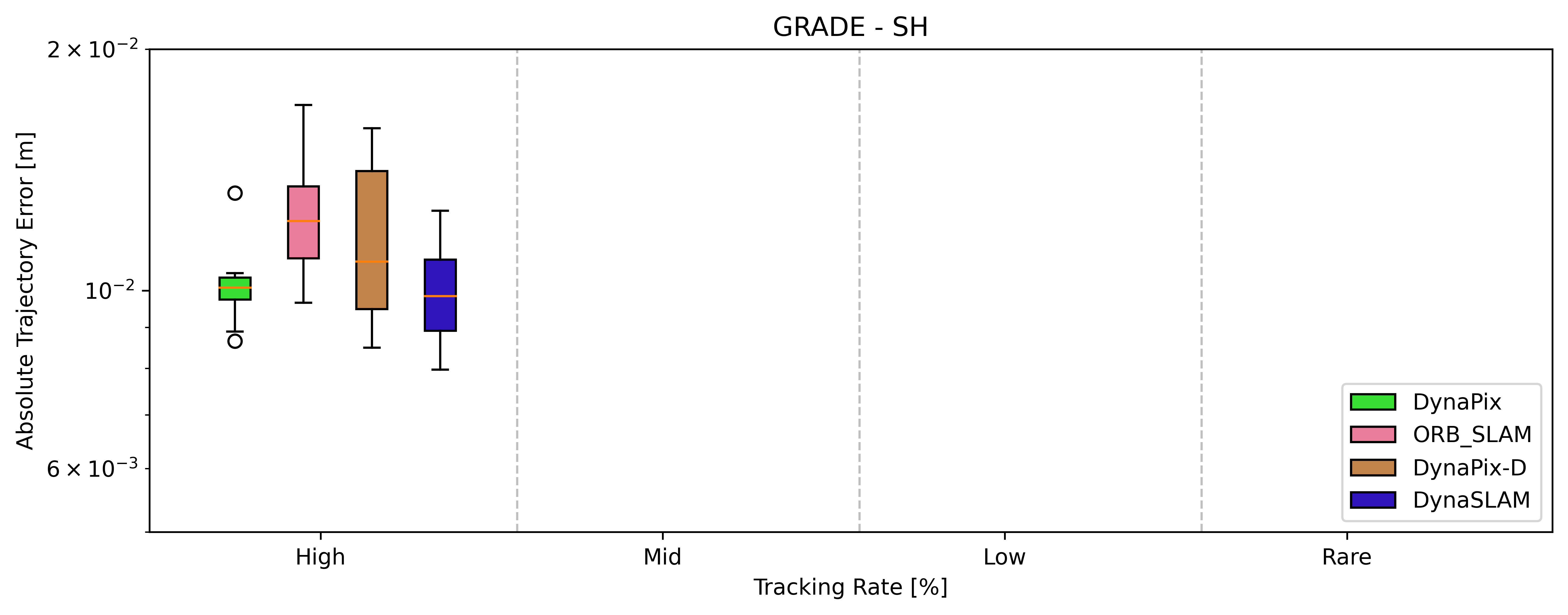
Figure xv: Box-Plot of results of the four methods tested on the SH sequence using the tracking rate buckets and the ATE results.

	DynaPix		ORB-SLAM2		DynaPix-D		DynaSLAM
	ATE [m]	TR	ATE [m]	TR	ATE [m]	TR	ATE [m]	TR
half	0.030	1.00	0.845	0.71	0.023	1.00	0.028	1.00
	0.028	1.00	0.474	0.89	0.022	1.00	0.030	1.00
	0.032	1.00	0.688	0.83	0.023	1.00	0.030	1.00
	0.028	1.00	0.574	0.81	0.022	1.00	0.029	1.00
	0.031	1.00	0.370	0.82	0.024	1.00	0.030	1.00
	0.033	1.00	0.691	0.60	0.022	1.00	0.029	1.00
	0.027	1.00	0.718	0.73	0.023	1.00	0.030	1.00
	0.035	1.00	0.332	0.87	0.022	1.00	0.028	1.00
	0.031	1.00	0.837	0.70	0.023	1.00	0.031	1.00
	0.029	1.00	0.540	0.97	0.021	1.00	0.029	1.00
MEAN	0.030	1.00	0.607	0.79	0.023	1.00	0.029	1.00
STD	0.002	0.00	0.180	0.11	0.001	0.00	0.001	0.00

Table ix: All the 10 runs ATE and TR results of all four methods on the TUM-RGBD fr3_walking/halfsphere sequence.

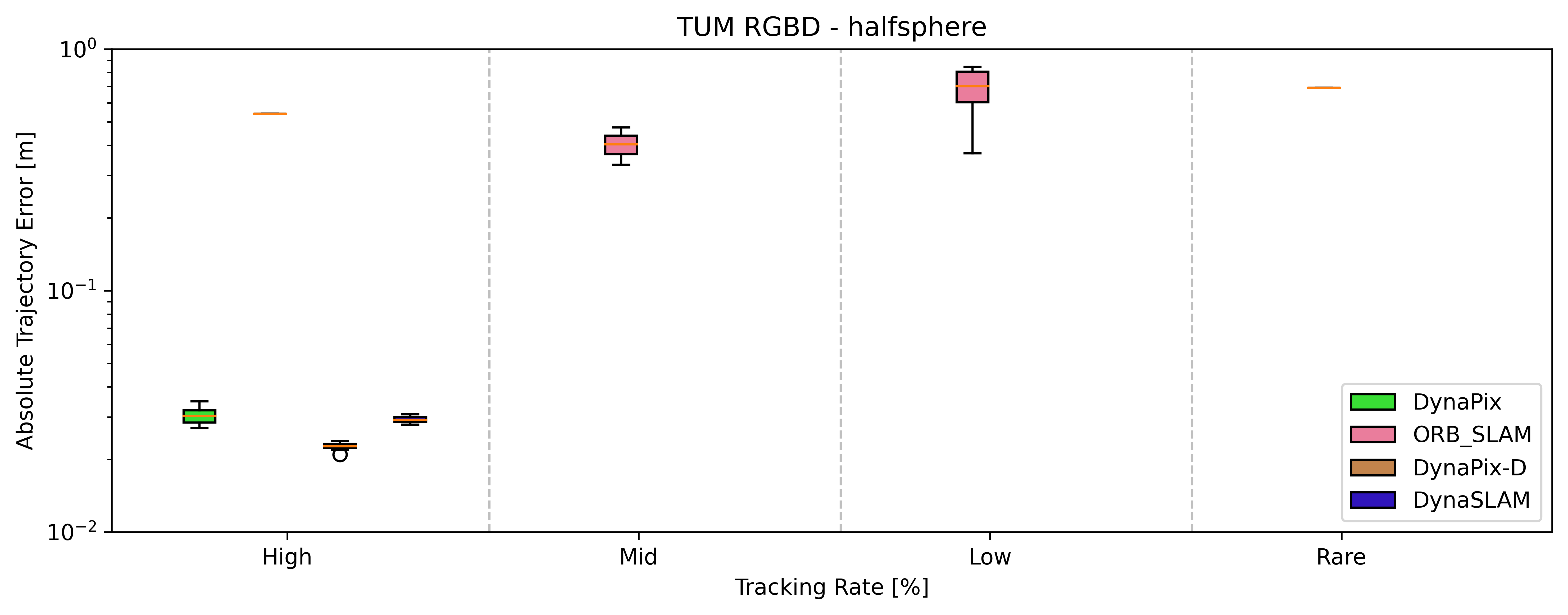
Figure xvi: Box-Plot of results of the four methods tested on the TUM-RGBD fr3_walking/halfsphere sequence using the tracking rate buckets and the ATE results.

	DynaPix		ORB-SLAM2		DynaPix-D		DynaSLAM
	ATE [m]	TR	ATE [m]	TR	ATE [m]	TR	ATE [m]	TR
static	0.012	1.00	0.021	1.00	0.006	1.00	0.007	0.99
	0.012	1.00	0.344	1.00	0.007	1.00	0.007	0.98
	0.014	1.00	0.405	1.00	0.007	1.00	0.007	0.98
	0.016	1.00	0.394	1.00	0.008	1.00	0.007	0.98
	0.009	1.00	0.351	1.00	0.006	1.00	0.007	0.98
	0.010	1.00	0.413	1.00	0.006	1.00	0.007	0.98
	0.011	1.00	0.437	1.00	0.006	1.00	0.007	0.98
	0.010	1.00	0.430	1.00	0.006	1.00	0.007	0.98
	0.011	1.00	0.384	1.00	0.007	1.00	0.007	0.98
	0.012	1.00	0.374	1.00	0.008	1.00	0.007	0.98
MEAN	0.012	1.00	0.355	1.00	0.007	1.00	0.007	0.98
STD	0.002	0.00	0.121	0.00	0.001	0.00	0.000	0.00

Table x: All the 10 runs ATE and TR results of all four methods on the TUM-RGBD fr3_walking/static sequence.

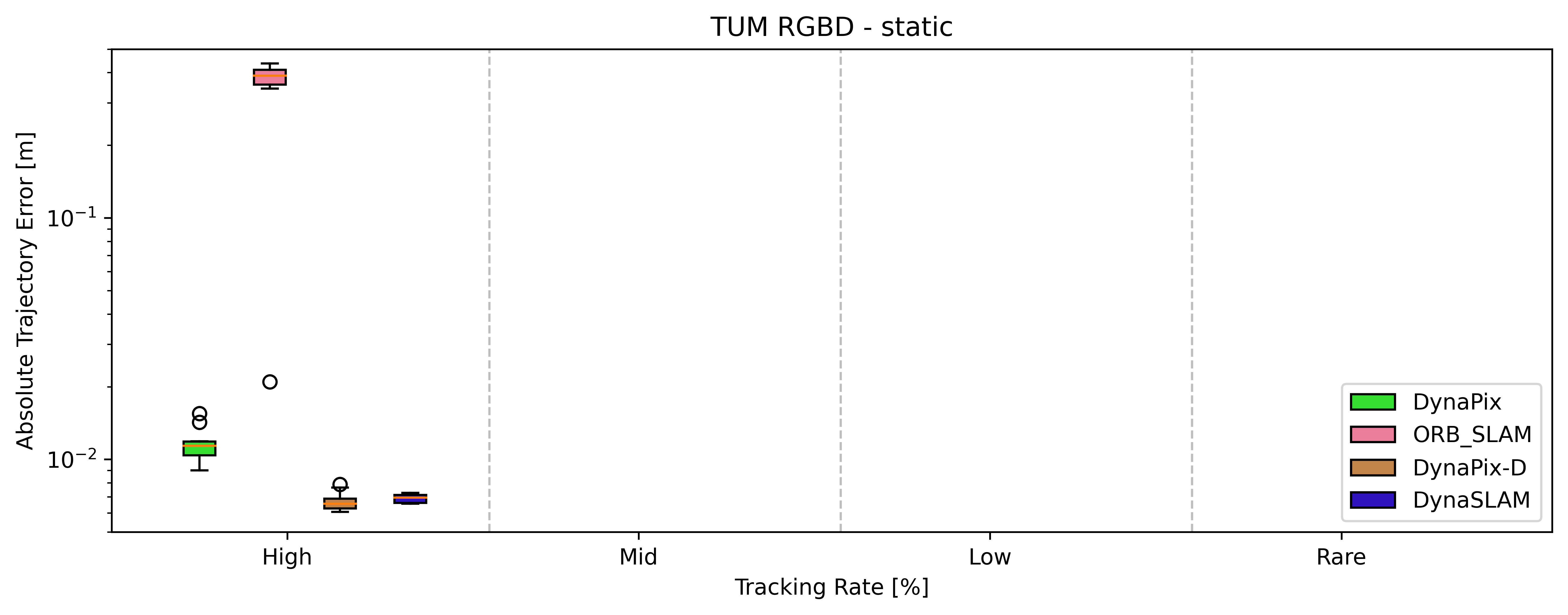
Figure xvii: Box-Plot of results of the four methods tested on the TUM-RGBD fr3_walking/static sequence using the tracking rate buckets and the ATE results.

	DynaPix		ORB-SLAM2		DynaPix-D		DynaSLAM
	ATE [m]	TR	ATE [m]	TR	ATE [m]	TR	ATE [m]	TR
rpy	0.039	1.00	0.844	0.98	0.035	1.00	0.037	0.81
	0.041	1.00	0.535	1.00	0.125	0.97	0.034	0.88
	0.040	1.00	0.725	1.00	0.032	1.00	0.049	0.88
	0.043	1.00	0.699	0.99	0.036	1.00	0.050	0.85
	0.041	1.00	0.672	0.99	0.170	0.98	0.043	0.92
	0.046	1.00	0.745	0.98	0.028	0.95	0.031	0.82
	0.043	1.00	0.691	0.98	0.237	1.00	0.051	0.83
	0.061	1.00	0.843	0.99	0.324	0.97	0.041	0.89
	0.040	1.00	0.955	1.00	0.036	1.00	0.034	0.85
	0.040	1.00	0.732	1.00	0.203	0.93	0.032	0.84
MEAN	0.043	1.00	0.744	0.99	0.123	0.98	0.040	0.86
STD	0.007	0.00	0.115	0.01	0.107	0.03	0.008	0.03

Table xi: All the 10 runs ATE and TR results of all four methods on the TUM-RGBD fr3_walking/rpy sequence.

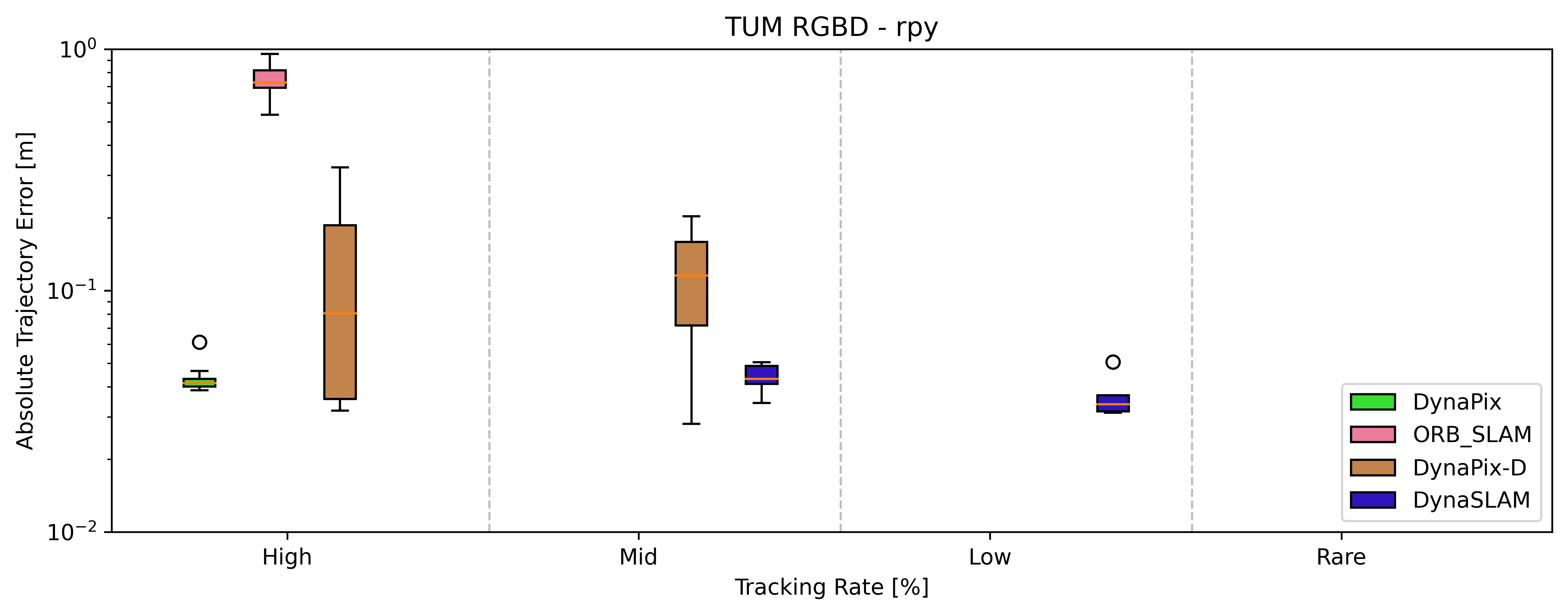
Figure xviii: Box-Plot of results of the four methods tested on the TUM-RGBD fr3_walking/rpy sequence using the tracking rate buckets and the ATE results.

	DynaPix		ORB-SLAM2		DynaPix-D		DynaSLAM
	ATE [m]	TR	ATE [m]	TR	ATE [m]	TR	ATE [m]	TR
xyz	0.018	1.00	0.792	0.80	0.013	1.00	0.016	0.92
	0.017	1.00	0.728	0.81	0.014	1.00	0.015	0.92
	0.018	1.00	0.630	0.78	0.013	1.00	0.016	0.92
	0.022	1.00	0.890	0.81	0.014	1.00	0.016	0.92
	0.019	1.00	0.738	0.85	0.014	1.00	0.015	0.92
	0.018	1.00	0.708	1.00	0.014	1.00	0.015	0.92
	0.017	1.00	0.575	0.68	0.014	1.00	0.015	0.92
	0.018	1.00	0.794	0.94	0.013	1.00	0.017	0.92
	0.016	1.00	0.621	0.68	0.013	1.00	0.017	0.92
	0.019	1.00	0.847	1.00	0.014	1.00	0.017	0.92
MEAN	0.018	1.00	0.732	0.84	0.014	1.00	0.016	0.92
STD	0.002	0.00	0.102	0.11	0.000	0.00	0.001	0.00

Table xii: All the 10 runs ATE and TR results of all four methods on the TUM-RGBD fr3_walking/xyz sequence.

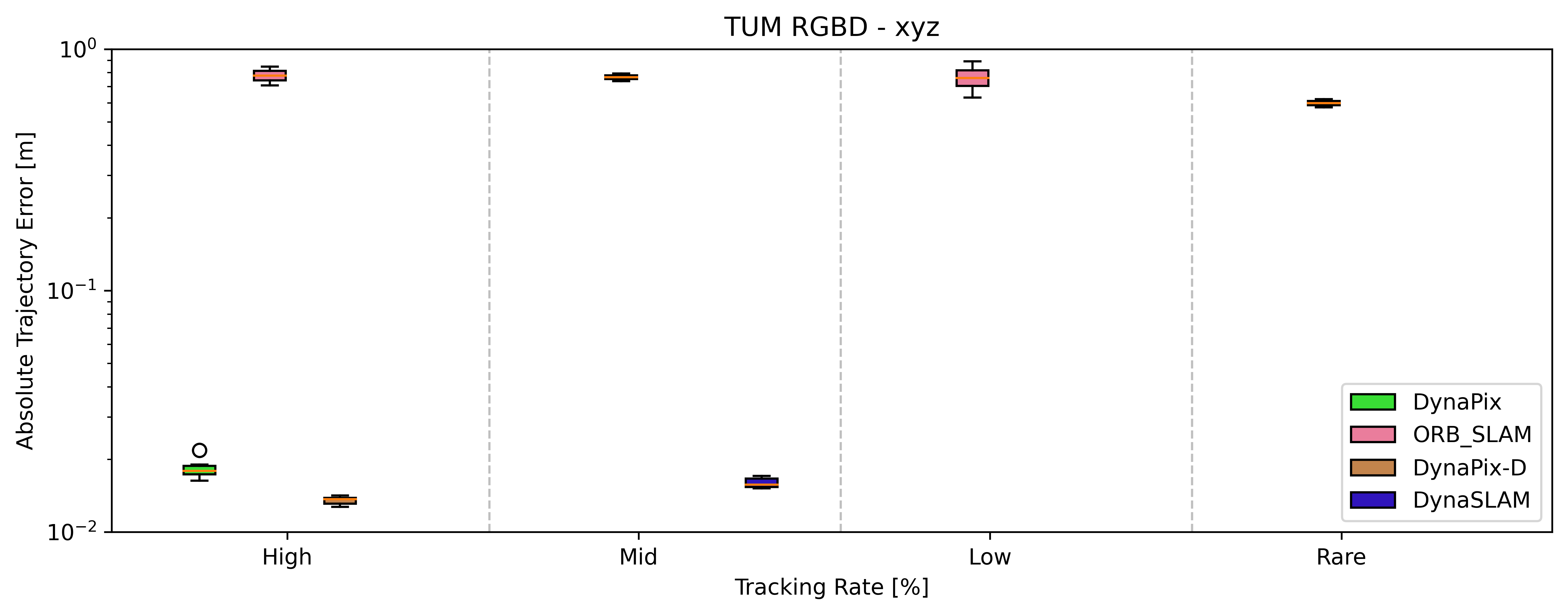
Figure xix: Box-Plot of results of the four methods tested on the TUM-RGBD fr3_walking/xyz sequence using the tracking rate buckets and the ATE results.

References

- Badrinarayanan et al. [2017] Vijay Badrinarayanan, Alex Kendall, and Roberto Cipolla. Segnet: A deep convolutional encoder-decoder architecture for image segmentation. IEEE Transactions on Pattern Analysis and Machine Intelligence, 39(12):2481–2495, 2017.
- Ballester et al. [2021] Irene Ballester, Alejandro Fontán, Javier Civera, Klaus H. Strobl, and Rudolph Triebel. Dot: Dynamic object tracking for visual slam. In 2021 IEEE International Conference on Robotics and Automation (ICRA), pages 11705–11711, 2021.
- Bescos et al. [2018] Berta Bescos, José M. Fácil, Javier Civera, and José Neira. Dynaslam: Tracking, mapping, and inpainting in dynamic scenes. IEEE Robotics and Automation Letters, 3(4):4076–4083, 2018.
- Bescos et al. [2021] Berta Bescos, Carlos Campos, Juan D. Tardós, and José Neira. Dynaslam ii: Tightly-coupled multi-object tracking and slam. IEEE Robotics and Automation Letters, 6(3):5191–5198, 2021.
- Bideau and Learned-Miller [2016] Pia Bideau and Erik Learned-Miller. It’s moving! a probabilistic model for causal motion segmentation in moving camera videos. In Computer Vision – ECCV 2016, pages 433–449, Cham, 2016. Springer International Publishing.
- Bojko et al. [2021] Adrian Bojko, Romain Dupont, Mohamed Tamaazousti, and Hervé Le Borgne. Learning to segment dynamic objects using slam outliers. In 2020 25th International Conference on Pattern Recognition (ICPR), pages 9780–9787, 2021.
- Bojko et al. [2022] Adrian Bojko, Romain Dupont, Mohamed Tamaazousti, and Herve Le Borgne. Self-improving slam in dynamic environments: Learning when to mask. In 33rd British Machine Vision Conference 2022, BMVC 2022, London, UK, November 21-24, 2022. BMVA Press, 2022.
- Bonetto et al. [2023a] Elia Bonetto, Chenghao Xu, and Aamir Ahmad. Grade: Generating realistic animated dynamic environments for robotics research. arXiv preprint arXiv:2303.04466, 2023a.
- Bonetto et al. [2023b] Elia Bonetto, Chenghao Xu, and Aamir Ahmad. Simulation of Dynamic Environments for SLAM. In ICRA2023 Workshop on Active Methods in Autonomous Navigation, 2023b.
- Bresson et al. [2017] Guillaume Bresson, Zayed Alsayed, Li Yu, and Sébastien Glaser. Simultaneous localization and mapping: A survey of current trends in autonomous driving. IEEE Transactions on Intelligent Vehicles, 2(3):194–220, 2017.
- Brissman et al. [2023] Emil Brissman, Joakim Johnander, Martin Danelljan, and Michael Felsberg. Recurrent graph neural networks for video instance segmentation. International Journal of Computer Vision, 131(2):471–495, 2023.
- Bujanca et al. [2021] Mihai Bujanca, Xuesong Shi, Matthew Spear, Pengpeng Zhao, Barry Lennox, and Mikel Luján. Robust slam systems: Are we there yet? In 2021 IEEE/RSJ International Conference on Intelligent Robots and Systems (IROS), pages 5320–5327, 2021.
- Cadena et al. [2016] Cesar Cadena, Luca Carlone, Henry Carrillo, Yasir Latif, Davide Scaramuzza, José Neira, Ian Reid, and John J. Leonard. Past, present, and future of simultaneous localization and mapping: Toward the robust-perception age. IEEE Transactions on Robotics, 32(6):1309–1332, 2016.
- Campos et al. [2021] Carlos Campos, Richard Elvira, Juan J. Gómez Rodríguez, José M. M. Montiel, and Juan D. Tardós. Orb-slam3: An accurate open-source library for visual, visual–inertial, and multimap slam. IEEE Transactions on Robotics, 37(6):1874–1890, 2021.
- Chacon-Murguia and Guzman-Pando [2022] Mario I Chacon-Murguia and Abimael Guzman-Pando. Moving object detection in video sequences based on a two-frame temporal information cnn. Neural Processing Letters, pages 1–25, 2022.
- Cheng et al. [2020] Jiyu Cheng, Hong Zhang, and Max Q.-H. Meng. Improving visual localization accuracy in dynamic environments based on dynamic region removal. IEEE Transactions on Automation Science and Engineering, 17(3):1585–1596, 2020.
- Cheng et al. [2023] Shuhong Cheng, Changhe Sun, Shijun Zhang, and Dianfan Zhang. Sg-slam: A real-time rgb-d visual slam toward dynamic scenes with semantic and geometric information. IEEE Transactions on Instrumentation and Measurement, 72:1–12, 2023.
- Dey et al. [2012] Soumyabrata Dey, Vladimir Reilly, Imran Saleemi, and Mubarak Shah. Detection of independently moving objects in non-planar scenes via multi-frame monocular epipolar constraint. In Computer Vision–ECCV 2012: 12th European Conference on Computer Vision, Florence, Italy, October 7-13, 2012, Proceedings, Part V 12, pages 860–873. Springer, 2012.
- Ding et al. [2022] Shuangrui Ding, Maomao Li, Tianyu Yang, Rui Qian, Haohang Xu, Qingyi Chen, Jue Wang, and Hongkai Xiong. Motion-aware contrastive video representation learning via foreground-background merging. In Proceedings of the IEEE/CVF Conference on Computer Vision and Pattern Recognition, pages 9716–9726, 2022.
- Dosovitskiy et al. [2015] A. Dosovitskiy, P. Fischer, E. Ilg, P. Häusser, C. Hazırbaş, V. Golkov, P. v.d. Smagt, D. Cremers, and T. Brox. Flownet: Learning optical flow with convolutional networks. In IEEE International Conference on Computer Vision (ICCV), 2015.
- Engel et al. [2018] J. Engel, V. Koltun, and D. Cremers. Direct sparse odometry. IEEE Transactions on Pattern Analysis and Machine Intelligence, 2018.
- He et al. [2023] Jiaming He, Mingrui Li, Yangyang Wang, and Hongyu Wang. Ovd-slam: An online visual slam for dynamic environments. IEEE Sensors Journal, 23(12):13210–13219, 2023.
- He et al. [2017] Kaiming He, Georgia Gkioxari, Piotr Dollár, and Ross Girshick. Mask r-cnn. In 2017 IEEE International Conference on Computer Vision (ICCV), pages 2980–2988, 2017.
- Hu et al. [2022] Xinggang Hu, Yunzhou Zhang, Zhenzhong Cao, Rong Ma, Yanmin Wu, Zhiqiang Deng, and Wenkai Sun. Cfp-slam: A real-time visual slam based on coarse-to-fine probability in dynamic environments. In 2022 IEEE/RSJ International Conference on Intelligent Robots and Systems (IROS), pages 4399–4406, 2022.
- Huang et al. [2022] Zhaoyang Huang, Xiaoyu Shi, Chao Zhang, Qiang Wang, Ka Chun Cheung, Hongwei Qin, Jifeng Dai, and Hongsheng Li. FlowFormer: A transformer architecture for optical flow. ECCV, 2022.
- Irani and Anandan [1998] M. Irani and P. Anandan. A unified approach to moving object detection in 2d and 3d scenes. IEEE Transactions on Pattern Analysis and Machine Intelligence, 20(6):577–589, 1998.
- Ji et al. [2021] Tete Ji, Chen Wang, and Lihua Xie. Towards real-time semantic rgb-d slam in dynamic environments. In 2021 IEEE International Conference on Robotics and Automation (ICRA), pages 11175–11181, 2021.
- Jinyu et al. [2019] Li Jinyu, Yang Bangbang, Chen Danpeng, Wang Nan, Zhang Guofeng, and Bao Hujun. Survey and evaluation of monocular visual-inertial slam algorithms for augmented reality. Virtual Reality & Intelligent Hardware, 1(4):386–410, 2019.
- Li et al. [2021] Ao Li, Jikai Wang, Meng Xu, and Zonghai Chen. Dp-slam: A visual slam with moving probability towards dynamic environments. Information Sciences, 556:128–142, 2021.
- Li et al. [2022] Zhen Li, Cheng-Ze Lu, Jianhua Qin, Chun-Le Guo, and Ming-Ming Cheng. Towards an end-to-end framework for flow-guided video inpainting. In IEEE Conference on Computer Vision and Pattern Recognition (CVPR), 2022.
- Liu et al. [2022] Jianheng Liu, Xuanfu Li, Yueqian Liu, and Haoyao Chen. Rgb-d inertial odometry for a resource-restricted robot in dynamic environments. IEEE Robotics and Automation Letters, 7(4):9573–9580, 2022.
- Liu et al. [2016] Wei Liu, Dragomir Anguelov, Dumitru Erhan, Christian Szegedy, Scott Reed, Cheng-Yang Fu, and Alexander C Berg. Ssd: Single shot multibox detector. In Computer Vision–ECCV 2016: 14th European Conference, Amsterdam, The Netherlands, October 11–14, 2016, Proceedings, Part I 14, pages 21–37. Springer, 2016.
- Liu et al. [2019] Xingyu Liu, Charles R. Qi, and Leonidas J. Guibas. Flownet3d: Learning scene flow in 3d point clouds. In Proceedings of the IEEE/CVF Conference on Computer Vision and Pattern Recognition (CVPR), 2019.
- Liu and Zhou [2022] Yu Liu and Zhiyu Zhou. Optical flow-based stereo visual odometry with dynamic object detection. IEEE Transactions on Computational Social Systems, pages 1–13, 2022.
- Lu et al. [2022] Yu Lu, Zhisheng Zhang, Haiying Wen, Min Dai, and Jing Xu. Rgb-d slam using scene flow in dynamic environments. In 2022 28th International Conference on Mechatronics and Machine Vision in Practice (M2VIP), pages 1–6, 2022.
- Meunier et al. [2023] Etienne Meunier, Anaïs Badoual, and Patrick Bouthemy. Em-driven unsupervised learning for efficient motion segmentation. IEEE Transactions on Pattern Analysis and Machine Intelligence, 45(4):4462–4473, 2023.
- Mirzaei et al. [2023] Ashkan Mirzaei, Tristan Aumentado-Armstrong, Konstantinos G. Derpanis, Jonathan Kelly, Marcus A. Brubaker, Igor Gilitschenski, and Alex Levinshtein. SPIn-NeRF: Multiview segmentation and perceptual inpainting with neural radiance fields. In CVPR, 2023.
- Mur-Artal and Tardós [2017] Raúl Mur-Artal and Juan D. Tardós. ORB-SLAM2: an open-source SLAM system for monocular, stereo and RGB-D cameras. IEEE Transactions on Robotics, 33(5):1255–1262, 2017.
- Niklaus and Liu [2020] Simon Niklaus and Feng Liu. Softmax splatting for video frame interpolation. In Proceedings of the IEEE/CVF Conference on Computer Vision and Pattern Recognition, pages 5437–5446, 2020.
- Qin et al. [2018] Tong Qin, Peiliang Li, and Shaojie Shen. Vins-mono: A robust and versatile monocular visual-inertial state estimator. IEEE Transactions on Robotics, 34(4):1004–1020, 2018.
- Ramachandran et al. [2009] Mahesh Ramachandran, Ashok Veeraraghavan, and Rama Chellappa. Chapter 5 - video stabilization and mosaicing. In The Essential Guide to Video Processing, pages 109–140. Academic Press, Boston, 2009.
- Ranjan et al. [2019] Anurag Ranjan, Varun Jampani, Lukas Balles, Kihwan Kim, Deqing Sun, Jonas Wulff, and Michael J. Black. Competitive collaboration: Joint unsupervised learning of depth, camera motion, optical flow and motion segmentation. In Proceedings of the IEEE/CVF Conference on Computer Vision and Pattern Recognition (CVPR), 2019.
- Redmon and Farhadi [2018] Joseph Redmon and Ali Farhadi. Yolov3: An incremental improvement. arXiv, 2018.
- Saputra et al. [2018] Muhamad Risqi U Saputra, Andrew Markham, and Niki Trigoni. Visual slam and structure from motion in dynamic environments: A survey. ACM Computing Surveys (CSUR), 51(2):1–36, 2018.
- Scona et al. [2018] Raluca Scona, Mariano Jaimez, Yvan R. Petillot, Maurice Fallon, and Daniel Cremers. Staticfusion: Background reconstruction for dense rgb-d slam in dynamic environments. In 2018 IEEE International Conference on Robotics and Automation (ICRA), pages 3849–3856, 2018.
- Shen et al. [2023] Shihao Shen, Yilin Cai, Wenshan Wang, and Sebastian Scherer. Dytanvo: Joint refinement of visual odometry and motion segmentation in dynamic environments. In 2023 IEEE International Conference on Robotics and Automation (ICRA), pages 4048–4055. IEEE, 2023.
- Shi et al. [2020] Xuesong Shi, Dongjiang Li, Pengpeng Zhao, Qinbin Tian, Yuxin Tian, Qiwei Long, Chunhao Zhu, Jingwei Song, Fei Qiao, Le Song, et al. Are we ready for service robots? the openloris-scene datasets for lifelong slam. In 2020 IEEE international conference on robotics and automation (ICRA), pages 3139–3145. IEEE, 2020.
- Song et al. [2022] Seungwon Song, Hyungtae Lim, Alex Junho Lee, and Hyun Myung. Dynavins: A visual-inertial slam for dynamic environments. IEEE Robotics and Automation Letters, 7(4):11523–11530, 2022.
- Sturm et al. [2012] J. Sturm, N. Engelhard, F. Endres, W. Burgard, and D. Cremers. A benchmark for the evaluation of rgb-d slam systems. In Proc. of the International Conference on Intelligent Robot Systems (IROS), 2012.
- Sun et al. [2018a] Deqing Sun, Xiaodong Yang, Ming-Yu Liu, and Jan Kautz. PWC-Net: CNNs for optical flow using pyramid, warping, and cost volume. In CVPR, 2018a.
- Sun et al. [2017] Yuxiang Sun, Ming Liu, and Max Q-H Meng. Improving rgb-d slam in dynamic environments: A motion removal approach. Robotics and Autonomous Systems, 89:110–122, 2017.
- Sun et al. [2018b] Yuxiang Sun, Ming Liu, and Max Q-H Meng. Motion removal for reliable rgb-d slam in dynamic environments. Robotics and Autonomous Systems, 108:115–128, 2018b.
- Turker and Eksioglu [2022] Anil Turker and Ender M. Eksioglu. A fully convolutional encoder-decoder network for moving object segmentation. In 2022 International Conference on INnovations in Intelligent SysTems and Applications (INISTA), pages 1–6, 2022.
- Wang et al. [2021] Chenjie Wang, Bin Luo, Yun Zhang, Qing Zhao, Lu Yin, Wei Wang, Xin Su, Yajun Wang, and Chengyuan Li. Dymslam: 4d dynamic scene reconstruction based on geometrical motion segmentation. IEEE Robotics and Automation Letters, 6(2):550–557, 2021.
- Wang et al. [2020] Wenshan Wang, Delong Zhu, Xiangwei Wang, Yaoyu Hu, Yuheng Qiu, Chen Wang, Yafei Hu, Ashish Kapoor, and Sebastian Scherer. Tartanair: A dataset to push the limits of visual slam. In 2020 IEEE/RSJ International Conference on Intelligent Robots and Systems (IROS), pages 4909–4916, 2020.
- Wang et al. [2022] Yanan Wang, Kun Xu, Yaobin Tian, and Xilun Ding. Drg-slam: A semantic rgb-d slam using geometric features for indoor dynamic scene. In 2022 IEEE/RSJ International Conference on Intelligent Robots and Systems (IROS), pages 1352–1359, 2022.
- Wu et al. [2022] Wenxin Wu, Liang Guo, Hongli Gao, Zhichao You, Yuekai Liu, and Zhiqiang Chen. Yolo-slam: A semantic slam system towards dynamic environment with geometric constraint. Neural Computing and Applications, pages 1–16, 2022.
- Wu et al. [2020] Xingming Wu, Lingkun Kong, Haosong Yue, Jianhua Wang, Fanghong Guo, and Weihai Chen. A robust slam towards dynamic scenes involving non-rigid objects. In 2020 15th IEEE Conference on Industrial Electronics and Applications (ICIEA), pages 1641–1646, 2020.
- Yang and Ramanan [2021] Gengshan Yang and Deva Ramanan. Learning to segment rigid motions from two frames. In CVPR, 2021.
- Yu et al. [2018] Chao Yu, Zuxin Liu, Xin-Jun Liu, Fugui Xie, Yi Yang, Qi Wei, and Qiao Fei. Ds-slam: A semantic visual slam towards dynamic environments. In 2018 IEEE/RSJ International Conference on Intelligent Robots and Systems (IROS), pages 1168–1174, 2018.
- Zhang et al. [2022] Jiacheng Zhang, Mingyu Gao, Zhiwei He, and Yuxiang Yang. Dcs-slam: A semantic slam with moving cluster towards dynamic environments. In 2022 IEEE International Conference on Robotics and Biomimetics (ROBIO), pages 1923–1928, 2022.
- Zhang et al. [2020] Tianwei Zhang, Huayan Zhang, Yang Li, Yoshihiko Nakamura, and Lei Zhang. Flowfusion: Dynamic dense rgb-d slam based on optical flow. In 2020 IEEE International Conference on Robotics and Automation (ICRA), pages 7322–7328, 2020.
- Zhong et al. [2018] Fangwei Zhong, Sheng Wang, Ziqi Zhang, China Chen, and Yizhou Wang. Detect-slam: Making object detection and slam mutually beneficial. In 2018 IEEE Winter Conference on Applications of Computer Vision (WACV), pages 1001–1010, 2018.
- Zhong et al. [2022] Yuanhong Zhong, Shuangshuang Hu, Guan Huang, Long Bai, and Qimin Li. Wf-slam: A robust vslam for dynamic scenarios via weighted features. IEEE Sensors Journal, 22(11):10818–10827, 2022.