Present address: ]Department of Biosystems Science and Engineering (D-BSSE), ETH Zurich, CH-4058 Basel, Switzerland
Evolution of cooperation in deme-structured populations on graphs
Abstract
Understanding how cooperation can evolve in populations despite its cost to individual cooperators is an important challenge. Models of spatially structured populations with one individual per node of a graph have shown that cooperation, modeled via the prisoner’s dilemma, can be favored by natural selection. These results depend on microscopic update rules, which determine how birth, death and migration on the graph are coupled. Recently, we developed coarse-grained models of spatially structured populations on graphs, where each node comprises a well-mixed deme, and where migration is independent from division and death, thus bypassing the need for update rules. Here, we study the evolution of cooperation in these models in the rare migration regime, within the prisoner’s dilemma. We find that cooperation is not favored by natural selection in these coarse-grained models on graphs where overall deme fitness does not directly impact migration from a deme. This is due to a separation of scales, whereby cooperation occurs at a local level within demes, while spatial structure matters between demes.
I Introduction
Cooperation between individuals is commonly observed in living systems, at the cell scale Hunter91 ; axelrod81 ; celiker2013cellular ; mitchison2004t , between animals dugatkin1997cooperation ; raihani2012punishment ; chase1980cooperative ; dugatkin2000cheating , and in human societies johnson2003puzzle ; rand2013human ; puurtinen2009between . For instance, bacteria often produce diffusible resources (e.g. enzymes, toxins or signaling molecules) that can benefit neighboring bacteria, including those that do not produce this resources (cheaters) Borenstein13 ; Cremer19 . Because producing these resources is generally costly, natural selection a priori works against the producers of public goods, and favors cheaters. Therefore, understanding how cooperation can evolve and spread is an important question Wingreen06 ; Cremer19 , which has led to intense debates. Kin selection can lead to the evolution of cooperation under some conditions Hamilton64a ; Hamilton64b : if the individuals that benefit from cooperation are related to cooperators, then cooperation can be selected even if it carries a cost. Spatial structure can also favor cooperation in some models ohtsuki2006evolutionary ; ohtsuki2006simple ; chuang2009simpson ; Melbinger10 ; Cremer12 ; Cremer19 . Since spatial structure generally entails that closely located individuals are genetically related, its ability to promote cooperation is related to kin selection Kay20 . In evolutionary game theory, individuals play games such as the prisoner’s dilemma doebeli2005 ; Turner99 or the snowdrift game doebeli2005 ; Gore09 using fixed strategies. Their fitnesses depend on the composition of the surrounding population, via the payoff they receive from the games played with their neighbors sigmund1999evolutionary ; weibull1997evolutionary ; traulsen2009stochastic ; hummert2014evolutionary . This allows to model cooperation in a straightforward way and to study its evolution. In these models, each individual is located on a node of a graph lieberman2005evolutionary , allowing to investigate the impact of complex spatial structures on the evolution of cooperation ohtsuki2006simple ; ohtsuki2006evolutionary . It was found that in the prisoner’s dilemma game, a cooperator mutant can be favored by natural selection in some graphs under specific update rules that prescribe how individuals are chosen to divide, die, and replace each other ohtsuki2006simple ; ohtsuki2006evolutionary .
Recently, we developed more general models of spatially structured populations on graphs, where each node comprises a well-mixed deme instead of a single individual, and where migration between demes is independent from division and death marrec2021toward ; Abbara23 . These models therefore do not require an update rule, contrary to other models with demes on graphs Houchmandzadeh11 ; yagoobi2021fixation ; yagoobi2023 . We showed that for mutants with constant (non-frequency-dependent) fitness, some spatial structures with specific migration asymmetries can amplify natural selection in the regime of rare migration marrec2021toward . We further found that suppression of selection is pervasive with more frequent migrations, in the branching process regime Abbara23 . Importantly, these results do not depend on update rules, contrary to models with one individual per node where suppression or amplification of natural selection for a given graph strongly depends on the update rule choice Kaveh15 ; Pattni15 ; Hindersin15 ; tkadlec2020limits . In the rare migration regime, this dependence on update rules was replaced by a dependence on migration asymmetry, which can be experimentally tuned and measured, while update rules model assumptions about the microscopic dynamics at the cell scale, which are generally not strictly followed by natural or experimental populations.
Can spatial structure favor the evolution of cooperation in these deme-structured models, as in models with one individual per node of the graph? To address these questions, we consider the prisoner’s dilemma in spatially structured populations within the frameworks of marrec2021toward ; Abbara23 . In these models, the fate of mutants is impacted by the choice of graph structure and specific migration rates between demes, but the average fitness of a deme does not directly impact the intensity of its outgoing (or incoming) migrations. In other words, selection is essentially soft Wallace75 , as we aimed for a minimal incorporation of spatial structure. Note however that cooperation can be favored via a coupling between composition and population size chuang2009simpson ; Melbinger10 ; Cremer12 ; Cremer19 .
We first lay out our models of deme-structured populations on graphs with cooperation in the case of the prisoner’s dilemma. Next, we consider a single cooperator (mutant), placed in a population entirely composed of defectors (wild-types), and we ask what the probability that it takes over (i.e. fixes) is. We address this question in different graphs, for rare migrations. We compare the fixation probability of a single cooperator to that of a single defector, and to that of a neutral mutant, to determine whether cooperation is favored or not. We also evaluate the impact of structure by comparing the fixation probability of a cooperator mutant in a structure to that in a well-mixed population with the same total size. We find that cooperators are not favored by natural selection in our models. The impact of spatial structure on their fixation probability reduces to that observed for mutants with fixed fitness disadvantage. This is due to a separation of scales, with cooperation occurring within demes, while spatial structure matters between demes. We make complete comparisons with models with one individual per node of the graph, including formal calculations in the Appendix, where we show the points that differ between these two classes of models.
II Model and methods
II.1 Spatially structured populations with demes on graphs
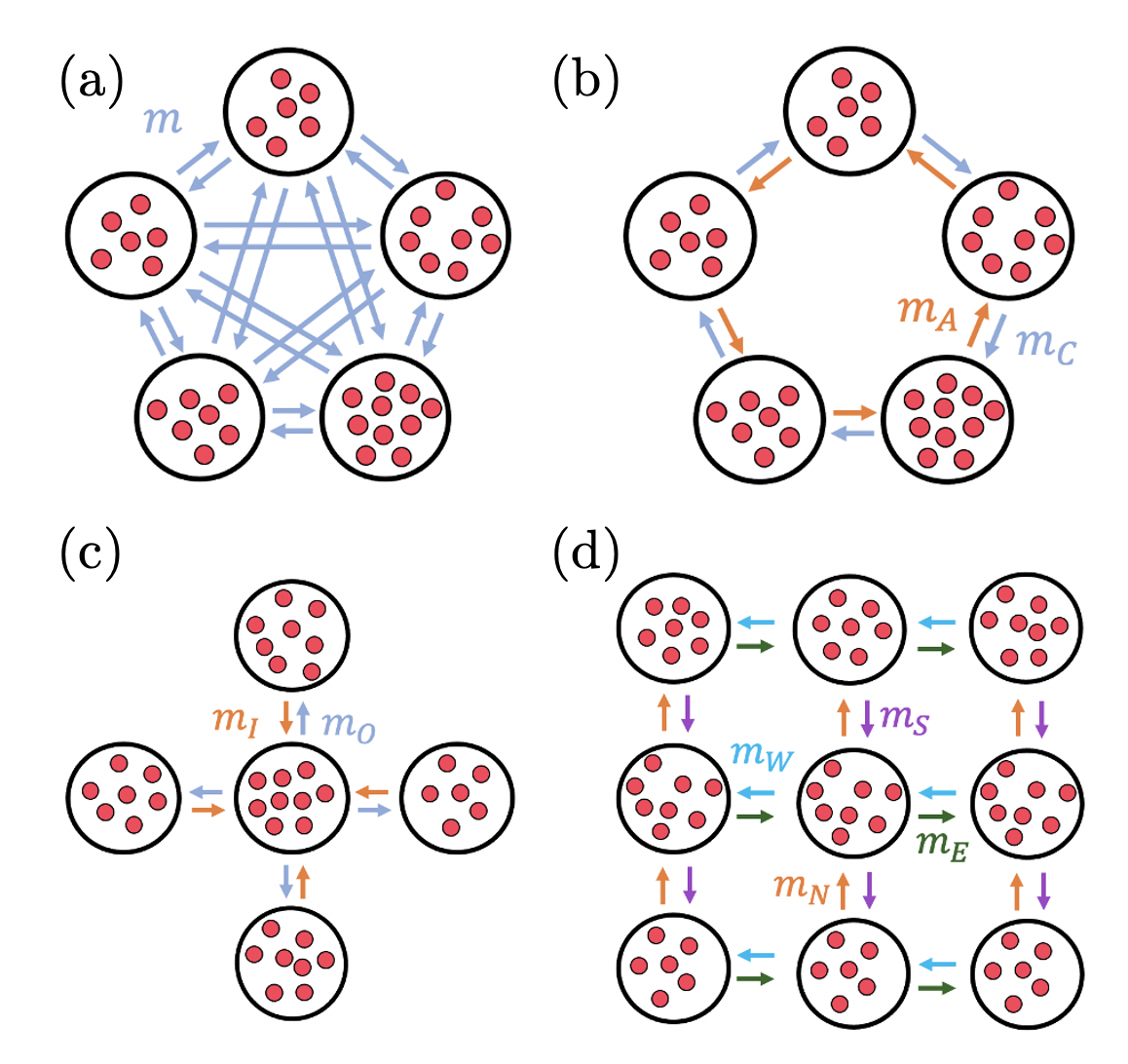
We model spatially structured populations on directed graphs. Each of the nodes of the graph contains a well-mixed subpopulation or deme. The specific graphs considered here are shown in Fig. 1. Two types of individuals make up the population: mutants () and wild-types (). We compare two different models, which differ by how deme size is regulated. In the first one, each individual can divide, die and migrate with given rates, deme sizes are limited by a carrying capacity, and we consider the regime where they fluctuate around a steady-state value marrec2021toward . In the second one, inspired by serial transfer experiments, the population undergoes an alternation of growth and bottleneck phases. Starting from a bottleneck state, each deme undergoes exponential growth, and then some individuals are sampled and migrate to form a new bottleneck state Abbara23 . Formally, the first model is close to a Moran model, but deme size is not strictly fixed marrec2021toward . Meanwhile, the second one is close to a Wright-Fisher model Abbara23 . We mainly study the first one, which is more directly comparable to models with one individual per node lieberman2005evolutionary ; ohtsuki2006evolutionary ; ohtsuki2006simple . The second model allows us to extend our results to more frequent migrations.
Within our models of spatial structure, we consider an evolutionary game theory setup that provides a simple description of cooperation, following ohtsuki2006evolutionary ; ohtsuki2006simple ; traulsen2009stochastic . Our two types of individuals then correspond to cooperators and defectors, interacting within a prisoner’s dilemma with payoff matrix
| (1) |
where . If a cooperator interacts with another cooperator, then both receive a benefit but also lose a cost ; this yields in the upper left corner of . If a cooperator interacts with a defector, then the cooperator does not receive anything, but it loses because of the interaction (upper right corner), while the defector receives (bottom left corner). Finally, if two defectors interact, both get 0. Note that here, being a cooperator or a defector in our model is an intrinsic (genetic) characteristic of an individual. Individual fitnesses are expressed as where is the intensity of selection and the total payoff received by the individual upon interactions with all its partners. We will usually consider cooperators as mutants () and defectors as wild-types (), and ask how likely it is that cooperator mutants take over.
We consider that interactions between individuals occur inside demes, which are well-mixed. Thus, each individual interacts with all other individuals in the same deme. Denoting by the number of mutants in a deme of size , the payoff for a mutant individual and for a wild-type individual in this deme read traulsen2009stochastic :
| (2) |
In these expressions, is the fraction of mutants among the individuals that a mutant of focus can interact with (i.e. all but itself), while is the fraction of wild-types among them. Similarly, is the fraction of mutants among the individuals that a wild-type of focus can interact with. In each of our two models, fitness can be expressed from these payoffs, giving rise to frequency-dependent fitnesses (see below).
II.2 Model with carrying capacities
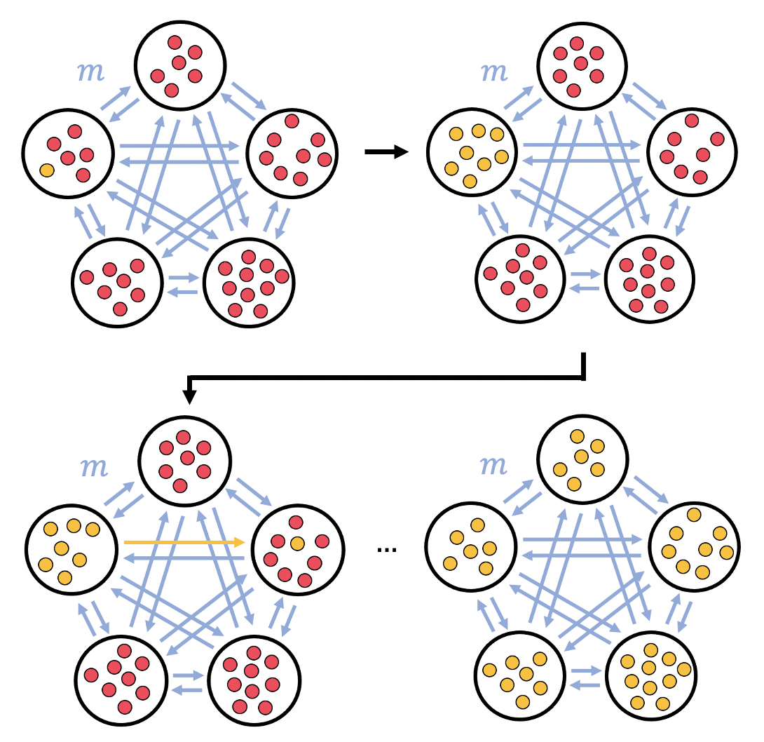
We first consider the model introduced in marrec2021toward . In this model, each deme has maximum carrying capacity . Besides, each individual has fitness or , and death rate , as we focus on selection on division. Here, fitness represents the maximal division rate of microorganisms, reached in exponential growth. The division rate of individuals of type in deme is given by the logistic function , where is the number of individuals in deme . As in marrec2021toward , we focus on the rare migration regime, where fixation or extinction within a deme occurs on much shorter time scales than migrations (see Fig. 2). In this regime, we describe the evolution of the microbial population as a Markov process where each event is a migration and where each deme is either fully mutant or fully wild-type Slatkin81 ; marrec2021toward . Note that we will present an extension to more frequent migrations using our second model (see below). We focus on the regime where deme sizes fluctuate weakly around their deterministic steady-state value (where we have neglected differences between and , which is acceptable for weak selection, and where we have neglected migrations, which is acceptable if they are rare). Note that the deterministic steady-state size is equal to the maximum carrying capacity if . In what follows, we will refer to as the deme carrying capacity, for simplicity. We approximate the fixation process of a type within a deme by a Moran process moran1958random ; ewens2004mathematical for a population of size , thus neglecting size fluctuations. Here, we implement logistic regulation in the division rate, which decreases if grows. Appendix C briefly discusses a variant where it is instead implemented in the death rate. Our conclusions are not affected.
Denoting by the number of mutants in a deme of size as above, the frequency-dependent fitness for a mutant individual and for a wild-type individual in this deme read:
| (3) |
where payoffs and are given by Eq. (2). Under this convention, where fitnesses depend linearly on payoffs, we will focus on the weak selection regime defined by and , where both and are close to the base fitness ohtsuki2006simple ; ohtsuki2006evolutionary . We will then briefly discuss an alternative convention where fitnesses depend exponentially on payoffs Traulsen08 , which allows an extension of our results beyond the weak selection regime.
We perform analytical calculations and stochastic simulations. For the latter, we use a Gillespie algorithm gillespie1976general ; gillespie1977exact ; marrec2021toward , described in detail in Appendix D. We will refer to this model in figures as the “carrying-capacity” (C. C.) one.
II.3 Model with serial dilutions
Recently, in Ref. Abbara23 , we introduced a new model of spatially structured populations on graphs, directly inspired by the batch culture setups with serial transfers that are used in many evolution experiments Lenski91 ; Elena03 ; Good17 ; Kryazhimskiy12 ; Nahum15 ; France19 ; Chen20 ; Kassen and are important in ecology Erez20 . This serial dilution model is a variant of the Wright-Fisher model, and features demes placed on the nodes of a graph with possible migrations along its edges, like the carrying-capacity model defined above. Each deme holds a well-mixed subpopulation, and within-deme interactions implement cooperation between individuals following the payoff matrix (1). In this model, all demes have the same bottleneck size , and repeatedly undergo a two-step process. To clarify notations, quantities common to the two models will be denoted with a prime for the serial dilution model.
-
1.
First, subpopulations grow exponentially in each deme during a fixed growth time . Time within this growth phase is denoted by . Starting at from mutants and wild-types in a deme at bottleneck, such that , these numbers grow as:
(4) with rates and reading
(5) Here is a shorthand for the payoff given in Eq. (2), with population size [and similarly for ]. The growth rates in Eq. (5) are chosen to have a similar form to the fitnesses given in Eq. (3). Here too, the payoffs obtained from the prisoner’s dilemma within demes directly impact the ability of cells to divide.
-
2.
Then, a dilution and migration step occurs (see details in Section B of the Appendix), bringing the system to a new bottleneck state. For each deme, we perform a multinomial sampling to pick exactly individuals that form the new bottleneck state of this deme. These incoming individuals are sampled from all demes, according to migration probabilities (all incoming migration probabilities to a given deme sum to 1).
In addition to bridging with experiments, this model has the advantage of facilitating the treatment of frequent migrations. Indeed, in our carrying capacity model under frequent asymmetric migrations, some demes can have a steady-state size that exceeds , which prevents division there. Choosing a division rate independent from and a death rate proportional to would instead result in substantially faster turnover in these demes. These situations lack realism and strongly depend on the exact form of deme size regulation. The serial dilution model does not suffer from this drawback.
We perform stochastic simulations under this serial dilution model Abbara23 , and we refer to it in figures as the “dilution” one. Considering the serial dilution model allows us to test the robustness of our conclusions from the carrying-capacity model in the rare migration regime, and to extend our study beyond this regime.
To quantitatively compare results from the two models, we choose the bottleneck size in the dilution model to be equal to the steady-state size of the demes in the carrying-capacity model. Furthermore, in the dilution model, we introduce the effective intensity of selection . Indeed, it plays the same role as the intensity of selection in the carrying-capacity model, see Section B.3 of the Appendix (in particular, the factor of 2 comes from the difference between a Moran and a Wright-Fisher description in the diffusion limit).
III Results
III.1 Fixation probability in a deme and in a structured population with rare migrations
In the rare migration regime, fixation of a mutant in the whole population starts by fixation in the deme where the mutant was introduced (see Methods and Fig. 2). Thus, we can write the fixation probability of a mutant in the structure as
| (6) |
where is the fixation probability of one mutant in a well-mixed deme where all other individuals are wild-type, while is the fixation probability of the mutant type in the whole population starting from one fully mutant deme and wild-type demes.
Let us first focus on , and let us compute it in the carrying-capacity model. Neglecting deme size fluctuations in the fixation process within a deme (see Methods) and denoting by the number of individuals in the deme, we can follow the calculation of traulsen2009stochastic , which yields:
| (7) |
Note that corresponds to the deterministic steady-state deme size , where we have neglected the impact of fitness differences on and used , as we focus on the weak-selection regime (this amounts to neglecting terms of order , which are explicitly written in marrec2021toward – this is acceptable if , which is realistic). Similarly, the fixation probability of one wild-type in a well-mixed deme where all other individuals are mutant reads
| (8) |
Inserting the fitness expressions from Eq. (3) into Eqs. (7) and (8), and performing an expansion in in the weak selection regime and yields:
| (9) | |||
| (10) |
We note that : we recover the result that in a well-mixed population, natural selection favours defectors over cooperators.
To calculate the fixation probability of a mutant in the whole structured population, we need to express the probability that the mutant type fixes, starting from one fully mutant deme, see Eq. (6). Importantly, depends on the specific graph that is considered for the structured population. Below, we focus on the simple graphs shown in Fig. 1, and investigate how each of them impacts the evolution of cooperation. To compute , we notice that in the rare migration regime, the state of the population can be fully described by specifying which demes are fully mutant and which ones are fully wild-type. Furthermore, this state evolves due to migration events, which may change it if they result into fixation in the destination deme. The evolution of the state of the population is a Markov chain Slatkin81 ; marrec2021toward .
III.2 Evolution of cooperation in the clique and cycle
Let us first consider the clique and the cycle, where all demes are equivalent. To compute , and more generally the fixation probability when starting from fully mutant demes (consecutive in the case of the cycle) and fully wild-type demes, we follow the method we used in marrec2021toward , which is based on traulsen2009stochastic . Briefly, we write down a recurrence relation on by discriminating over all possible outcomes of the first migration event: either increases by one if a mutant migrates to a wild-type deme and fixes there, or it decreases by one in the opposite case, or it stays constant in all other cases (see Appendix A.1 and marrec2021toward for details). Solving this recurrence relation yields
| (11) |
with
| (12) |
The reasoning made with frequency-independent fitness in marrec2021toward thus extends to the present case with cooperation, and accordingly, the formal expression of is the same in both cases. However, the expression of differs because the fixation probabilities within a deme are impacted by the cooperation model. In the present case, can be expressed using Eqs. (9) and (10). Note that Eq. (11) is independent from migration rates. In particular, in the case of the cycle, Eq. (11) does not depend on the ratio of the anticlockwise migration rate to the clockwise one , see Fig. 1.
In marrec2021toward , we further showed that all circulation graphs (such that the sum of incoming migration rates to any given deme is equal to the sum of outgoing ones from that deme), including the cycle, have the same fixation probability, thereby extending the circulation theorem which holds for graphs with one individual per node lieberman2005evolutionary . The circulation theorem further extends to the present case with cooperation. Indeed, the exact same proof as in marrec2021toward holds, albeit with a different . Therefore, all circulation graphs have the same fixation probability of cooperator mutants, given by Eqs. (11) and (12). We will henceforth denote it by .
Using Eqs. (9) and (10) to express Eq. (11) yields
| (13) |
which gives the fixation probability of a mutant in the whole population, using Eq. (6) and Eq. (9):
| (14) |
Importantly, this fixation probability is smaller than the neutral value for all : cooperation is never favored by natural selection in circulation graphs, including the clique or the cycle. It is also very similar to the fixation probability of a mutant in a well-mixed population of size [obtained from Eq. (9) by replacing with ] – both coincide for (see also marrec2021toward ).
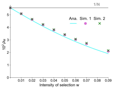
In Fig. 3(a), we compare numerical simulation results and analytical predictions for the fixation probability in the cycle. We find that stochastic simulation results do not depend on migration asymmetry , consistently with our analytical calculations of . A slight discrepancy can however be observed between analytical predictions and simulation results. It arises from the constant-size approximation we made to compute the analytical expressions of and , which are both involved in the expression of . Indeed, using Gillespie simulation results obtained on well-mixed demes for and instead of their analytical expressions for fixed size within the expression yields an excellent agreement with simulation results [see Fig. 3(a)].
In Fig. 3(b), we explore more frequent migrations, using the serial dilution model introduced above. Our simulation results suggest that the fixation probability for a cycle remains the same for more frequent migrations. Besides, as expected, matching the effective intensity of selection in this model to in our first carrying-capacity model, simulations from both models give close results for rare migrations. The rare migration analytical prediction for the dilution model is obtained with Eq. (11), but replacing and with their expressions and derived in the dilution model (see details in Section B of the Appendix). Note that Abbara23 extended the circulation theorem to the dilution model without cooperation, both for rare migrations, and for frequent migrations within the branching process approximation.
Our results stand in contrast to those of ohtsuki2006simple , where the present model of cooperation was studied in a cycle graph with one individual per node. There, it was found that cooperators could be favored by natural selection under the death-Birth (dB) and imitation update rules, but not under the Birth-death (Bd) update rule (the uppercase B indicates that selection on fitness happens at the birth step). Specifically, natural selection was found to favor cooperation in the dB case if ohtsuki2006simple . To understand the formal origin of this difference, we revisit the derivation of ohtsuki2006simple in Appendix A.1. The key difference is that in our model, cooperative interactions occur within a deme and are not involved in migration events. Conversely, in the model of ohtsuki2006simple , they impact the spread of mutants on the graph since birth, death and migration events are coupled via update rules.
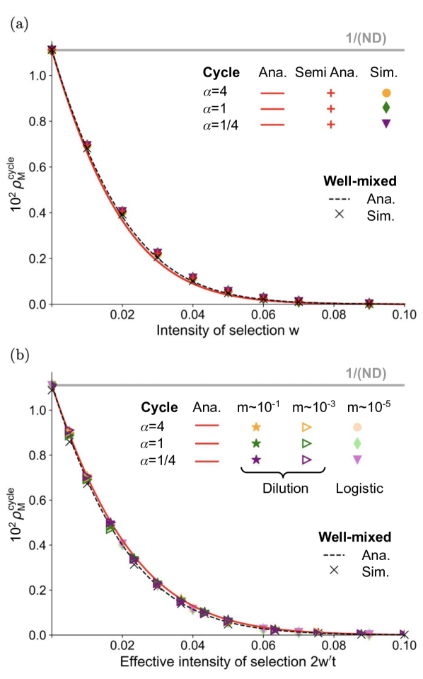
(b) Mutant fixation probability in the cycle versus effective intensity of selection in the dilution model, for different migration asymmetries and intensities. The solid red line represents the analytical prediction in the rare migration regime in the dilution model, from Eqs. (6,11), using Eqs. (52, 53) for and . The well-mixed population case (black dashed line) in the dilution model and simulations for the carrying-capacity (C. C.) model in the rare migration regime (versus ) are shown for comparison. Dilution simulation results are obtained over realizations for (, ) and = (4,1), (1,1) and (1,4).
In this figure, we consider demes with carrying capacity , death rate yielding steady-state size , and benefit and cost and . The well-mixed population holds individuals.
III.3 Evolution of cooperation in the star
Let us now consider the star graph, where the center sends out individuals to any leaf with rate , and receives individuals from any leaf with rate [see Fig. 1(c)]. This graph structure has been extensively studied for mutants with constant fitness. In evolutionary graph theory with one individual per node, the star amplifies or suppresses natural selection depending on the update rule lieberman2005evolutionary ; Kaveh15 ; Hindersin15 ; Pattni15 . For instance, it is an amplifier of selection using the Bd update rule, but a suppressor with the dB rule. In evolutionary graph theory with nodes containing subpopulations, the evolutionary outcome also depends on the specific update mechanism yagoobi2023 . In our model with rare migrations marrec2021toward that does not rely on a specific update rule, the star’s behavior depends on migration asymmetry , as amplifies selection while suppresses it. This same outcome holds for the rare migration regime in the serial dilution model Abbara23 . However, for more frequent migrations, the star becomes a suppressor for all migration asymmetries in the branching process regime Abbara23 . How does the star graph impact the fixation of a cooperator, in the rare migration regime and beyond?
To address this question, we extend the calculation of marrec2021toward to our cooperation model, and we express the fixation probability starting from one fully mutant deme, uniformly chosen among all demes, in the star graph. As in marrec2021toward , we obtain
| (15) |
where is given by Eq. (12), while is the ratio of the migration rate incoming to the center from a leaf , to that outgoing from the center to a leaf , see Fig. 1. Eq. (15) shows that migration asymmetry directly impacts the fixation probability in the star. In marrec2021toward , we demonstrated that the star amplifies natural selection for and suppresses it for . For , the fixation probability reduces to Eq. (11), as the star is then a circulation graph.
Using Eqs. (9) and (10) to express Eq. (15) yields
| (16) |
Studying the ratio between Eq. (III.3) and Eq. (13) shows that the fixation probability of a cooperator mutant is larger in the star than in the clique for (i.e. when the star behaves as a suppressor of selection marrec2021toward ) and smaller for (i.e. when the star behaves as an amplifier of selection marrec2021toward ). This result is confirmed by stochastic simulations in Fig. 4(a). These effects are purely due to the population structure and not to the cooperation model. In other words, what we find here holds as well for a deleterious mutant without frequency-dependent fitness (see marrec2021toward ). Simulations in Fig. 4(b) show that cooperation does not impact the star’s behavior in the dilution model either, compared to the case of mutants with constant fitness Abbara23 . Indeed, the rare migration regime recovers results from the carrying-capacity model, but as migrations become frequent, the star becomes a suppressor of natural selection regardless of migration asymmetry Abbara23 .
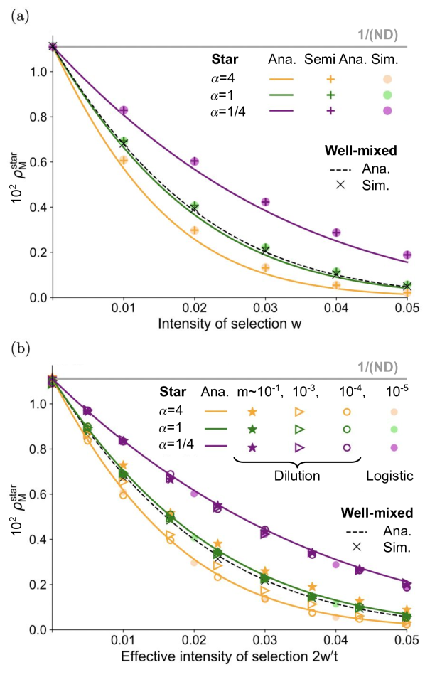
(b) Mutant fixation probability in the star for the dilution model versus effective intensity of selection , for different migration asymmetries and intensities. Simulations for the dilution model are obtained over realizations for (, ) and = (4,1), (1,1) and (1,4).
In both panels, analytical predictions in the rare migration regime use Eq. (15) instead of Eq. (11). They yield values close to the well-mixed case for =1 (green [middle] solid line), larger values for =1/4 (purple [upper] solid line), and smaller values for =4 (yellow [bottom] solid line).
III.4 Evolution of cooperation in the square lattice
In ohtsuki2006simple , a general rule for cooperation on graphs was found for the model with one individual per node, where interactions are defined by a specific update rule. The key result of ohtsuki2006simple is that under the death-Birth (dB) update rule, natural selection favours cooperators (i.e. mutant individuals here) if , where here is the average degree of the graph (i.e., the average number of neighbours per node). No such effect exists under the Bd update rule ohtsuki2006simple . In Appendix A.2, we revisit step-by-step the derivation of ohtsuki2006simple , which uses a pair approximation, and adapt it to our model. We find that the fixation probability starting from one fully mutant deme, given in Eq. (45), does not involve the average degree and that natural selection never favors cooperation. Again, the key differences are that in our model, birth, death and migration are all independent, and that cooperation occurs within demes.
The proof of ohtsuki2006simple is exact for Bethe lattices, i.e. infinite graphs without cycles where each individual has exactly neighbors. Graphs possessing this last property are said to be regular. Because Bethe lattices pose some difficulties for simulations, finite regular graphs, including square lattices, were simulated in ohtsuki2006simple , yielding good overall agreement with the prediction that cooperators are favored if . Thus motivated, here, we study the square lattice with demes shown in Fig. 1, adding periodic boundary conditions, so that each deme is connected to exactly 4 other demes. This graph is a circulation, since for each deme, the incoming migration rates sum to , and the outgoing ones too. Therefore, we predict that the fixation probability of a mutant in the rare migration regime is the same as in other circulation graphs (see Section III.2), and does not depend on migration asymmetry. Fig. 5(a) shows that our simulation results are in good agreement with this prediction. In addition, this result seems to extend to frequent migrations in the dilution model, see Fig. 5(b).
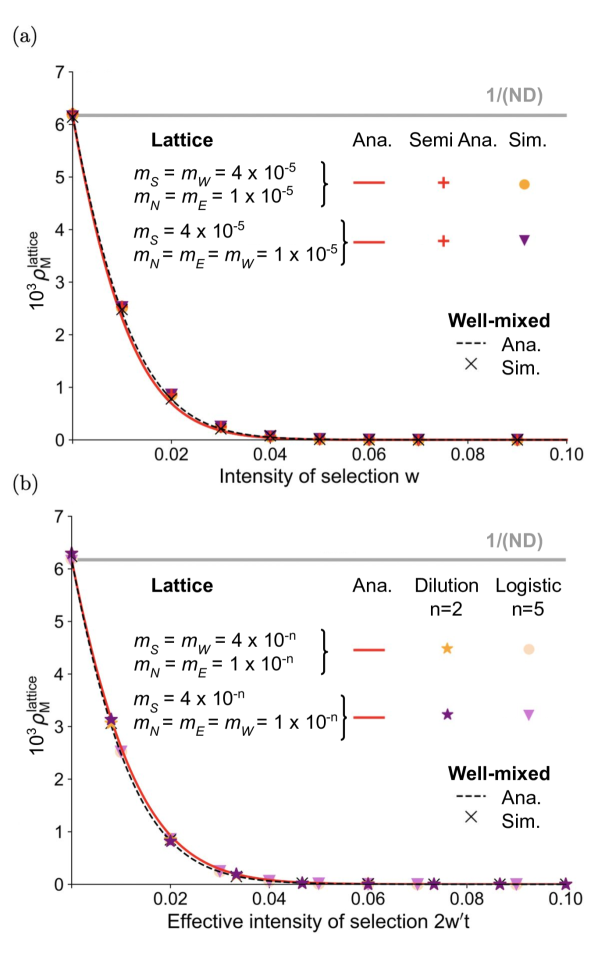
(b) Mutant fixation probability in the square lattice with periodic boundary conditions for the dilution model versus effective intensity of selection , for different migration asymmetries and intensities.
Here, we consider demes with carrying capacity and steady-state size . Other parameter values and conventions are the same as in Fig. 3. All simulation results are obtained over replicates.
III.5 Beyond weak selection
So far, we assumed that fitnesses depend linearly on payoffs [see Eq. (3)], and we remained in the weak selection regime where . This allowed us to give simple analytical expressions of fixation probabilities in demes, and to conduct a direct comparison with Refs. ohtsuki2006simple ; ohtsuki2006evolutionary .
It is analytically difficult to go beyond weak selection if fitnesses depend linearly on payoffs. However, Ref. Traulsen08 showed that calculations beyond the weak selection regime simplify if fitnesses depend exponentially on payoffs. This amounts to writing
| (17) |
where is a parameter that determines the intensity of selection (as in the linear case), instead of Eq. (3). Payoffs and remain expressed by Eq. (2).
Using the same reasoning as before, we obtain the same expressions for the probabilities of fixation of cooperator mutants in subdivided populations for rare migrations, namely Eq. (11) for the clique, the cycle, and all circulations, and Eq. (15) for the star. What changes is the expression of the fixation probabilities within demes, which now read Traulsen08
| (18) |
and
| (19) |
Their ratio, which enters Eq. (11) and Eq. (15), is:
| (20) |
where we neglected the dependence of steady-state deme size on fitness, which is acceptable if (see Methods and Ref. marrec2021toward ). Hence, this exponential convention for fitnesses yields simple analytical expressions of fixation probabilities for rare migrations in our model of spatially structured populations. Here, we assumed but not : in this sense, these results hold beyond weak selection. In addition, the first-order expansions of Eqs. (18) and (19) when and exactly match Eqs. (9) and (10), respectively, with standing in for . Thus, the exponential and the linear conventions for fitnesses are equivalent in the weak selection regime.
Importantly, because only the fixation probabilities within demes are modified by changing from linear to exponential fitnesses, our main conclusions remain valid in the exponential case. This includes our results for circulations and stars which are based respectively on Eq. (11) and Eq. (15), as well as our reasoning for general graphs based on the pair approximation in Appendix A.2. Our main result that natural selection does not favor cooperation in our model of spatially structured populations therefore extends beyond weak selection, at least to the regime where without needing .
IV Discussion
In all structures we considered, the fixation probability of a cooperator in a population of defectors is smaller than vice-versa. Thus, cooperation is never favored in our model. The reason for this is that cooperation only takes place within nodes. Migration events do not directly involve cooperation or any interaction between individuals from different demes, not even competition. Cooperation is therefore a local interaction. In contrast, cooperative interactions happen at the level of the graph in ohtsuki2006evolutionary . Indeed, each individual (placed on one node) interacts with its nearest neighbors on the graph, which affects its fitness and thus its probability of being picked at the birth step. This separation of scales entails that cooperation cannot be favored by natural selection in our model, including in other graphs, complex networks Chen08 , and structures with multiple network layers Zhang15 .
More formally, our model decouples migration, birth, and death events. In the rare migration regime, fixing in one deme and spreading to the whole spatially structured population happen on two different time scales. Because of this, fitnesses enter overall fixation probabilities only through the fixation probabilities in one well-mixed deme, namely and . Assuming that fitnesses depend linearly on payoffs, in the weak selection regime, we can compare Eqs. (9) and (10) to the fixation probabilities that would be obtained in the frequency-independent case, i.e. with a slightly deleterious mutant with fitness disadvantage satisfying , . We get a perfect mapping when choosing . Moreover, assuming that fitnesses depend exponentially on payoffs as in Section III.5, Eqs. (18) and (19) also match the frequency-independent fixation probabilities obtained in that convention with , and this holds beyond weak selection, assuming without needing . Thus, the fixation probabilities and have the same expression as with constant fitnesses, as long as we pick an effective fitness disadvantage for the mutant, which depends on the parameters of cooperation. This confirms that at the level of the whole structure, the frequency-dependence of the model does not matter. Because of this, cooperation cannot benefit from the specificities of the structure. Thus, our previous results regarding the impact of spatial structure on mutant fixation for constant fitnesses marrec2021toward ; Abbara23 extend to the present model with cooperation.
In our framework, selection is essentially soft, i.e. the contributions of demes are not affected by their average fitnesses Wallace75 . Indeed, in our dilution model, the total size of each deme after growth does not impact its contribution to the next bottleneck state. In our carrying-capacity model, the carrying capacity of each deme is fixed and independent of its composition, and equilibrium sizes depend only weakly on it. We implemented soft selection because we aimed to assess the impact of population structure in its most minimal form. A promising direction for future research would be to study such a model with hard selection. Indeed, in models where subpopulations contribute to the next bottleneck proportionally to their sizes, the fraction of cooperators can increasing overall despite decreasing within each subpopulation chuang2009simpson : this is known as the Simpson paradox blyth1972simpson ; simpson1951interpretation ; samuels1993simpson ; good1987amalgamation . Such a coupling between composition and population size can favor the evolution of cooperation Melbinger10 ; Cremer12 ; Cremer19 . It will thus be important to understand how this effect is impacted by graph structure. A first interesting step in this direction was conducted in Ref. Fu13 , which determined conditions under which cooperation can be favored at mutation-selection equilibrium, in a model with constant total population size but variable deme sizes.
In this context, we can summarize our results as follows. The ability of specific graphs and update rules to favor the evolution of cooperation in models with one individual per node of the graph ohtsuki2006evolutionary ; ohtsuki2006simple does not survive coarse-graining in a model with soft selection. This result does not arise from considering larger deme sizes, but from separating scales. Indeed, in our model, migration is independent from birth and death, and cooperation occurs locally within demes, while spatial structure matters between demes.
In addition to considering hard selection, possible extensions include addressing other ways through which migration may couple with cooperation Wu11 , studying other games such as the snowdrift game Gore09 , and explicitly modeling the dynamics of a diffusible resource Borenstein13 .
Appendix A Formal comparison with models with one individual per node
A.1 Cycle ohtsuki2006evolutionary
In ohtsuki2006evolutionary , evolutionary games, and especially the prisoner’s dilemma, were studied in the context of the cycle graph with one individual per node and with different update rules (birth-death, death-birth, imitation). Analytical expressions were obtained for the fixation probability of a cooperator in a population of defectors and vice-versa, in the weak-selection regime . The key result of ohtsuki2006evolutionary is that selection can favour cooperators over defectors for death-birth and imitation updates, but not birth-death updates. To understand the similarities and differences with our model, let us compare the derivations of the fixation probabilities in the cycle within each of the two models.
In our model with a well-mixed deme on each node of the cycle and migration events independent from birth and death events, and in the rare migration regime, let denote the number of fully mutant demes. Upon each migration event, the number of mutant demes can either increase by one with probability , due to a migration of one mutant individual to a wild-type deme and its subsequent fixation in it, or decrease by one with probability upon the opposite succession of events, or stay constant in all other cases. A recurrence relationship can then be written on the fixation probability in a cycle of demes starting from consecutive fully mutant demes. For this, one considers all the possibilities at the first migration event that occurs, which allows to relate to and . Solving this recurrence relationship yields
| (21) |
where , which is independent of . Therefore, Eq. (21) gives
| (22) |
A more detailed derivation (which is presented without frequency-dependent fitness, but extends to the present case) is given in marrec2021toward , and the general method is presented in traulsen2009stochastic . Note that the expression in Eq. (22) also holds in the case of the clique, where it can be obtained with an extremely similar derivation marrec2021toward .
In the model with one individual per node of a cycle with nodes considered in ohtsuki2006evolutionary , the same approach was employed to express the fixation probability of one mutant, yielding
| (23) |
which is formally equivalent to in our model (see Eq. (21)). However, in this model, , where (resp. ) represents the probability that the number of mutant nodes increases (resp. decreases) by one upon an update, takes different expressions depending on the update rule ohtsuki2006evolutionary . Indeed, with the birth-death update rule,
| (24) |
for , where (resp. ) is the fitness of a wild-type (resp. mutant) at the edge of the cluster of mutant nodes, i.e. which has a mutant neighbor and a wild-type neighbor. Here we expressed each fitness as where the total payoff received by an individual on the cycle is computed by summing the payoffs they receive from interactions with their two neighbors, with the payoff matrix in Eq. (1). We also used the fact that during the fixation process, starting from one mutant, there is a cluster of consecutive mutant nodes that cannot break. With the death-birth update rule, the fitnesses involved in depend on whether the mutant that was at an edge of the cluster of mutant nodes (individual 1) or its wild-type neighbor (individual 2) is selected to die. If individual 1 is selected to die, which can lead to a decrease of by one, the fitness of the wild-type (resp. mutant) neighbor of individual 1 is denoted by (resp. ). If individual 2 is selected to die, which can lead to an increase of by one, the fitness of the wild-type (resp. mutant) neighbor of individual 1 is denoted by (resp. ). We have
| (25) |
for . The expressions in Eqs. (24) and (25) differ for all , which leads to different probabilities of fixation under these two different update rules ohtsuki2006evolutionary .
This comparison of the derivation of fixation probabilities within our model and within that of ohtsuki2006evolutionary shows that the key difference is that in our model, migration events do not depend on birth or death and are thus decoupled from interactions between individuals, while in models with one individual per node, any move on the graph is coupled to birth and death via the update rule.
A.2 General graphs with pair approximation ohtsuki2006simple
While ohtsuki2006evolutionary focused on the cycle, ohtsuki2006simple derived a general rule for cooperation on graphs in the same model with one individual per node. The key result of ohtsuki2006simple is that under the death-birth (dB) update rule, natural selection favours cooperators (i.e. mutant individuals here) if , where here is the average degree of the graph (i.e., the average number of neighbours per node). No such effect exists under the Bd update rule ohtsuki2006simple . To understand the origin of the difference between these results and ours, we here follow the main analytical derivation of ohtsuki2006simple and adapt it to our model. Again, the key difference is that our model does not involve any update rule, as birth, death and migration are all independent. We will point out where this matters.
Following ohtsuki2006simple , let (resp. ) denote the frequency of fully mutant (resp. wild-type ) demes in a given graph comprising nodes. In our model, each of these nodes contains a well-mixed deme, while it comprises a single individual in ohtsuki2006simple . Let us also introduce the frequencies , , and of neighbouring , , and pairs of demes, and the conditional probability to find an deme at a certain position given that one randomly chosen nearest-neighbour of this deme (i.e. a deme connected to it by an edge) is a deme. We focus on the rare migration regime. As in ohtsuki2006simple , we will make a pair approximation where only the pair correlation is accounted for, meaning that higher-order correlations are fully determined by these pair correlations. The pair approximation requires Bethe lattices (or Cayley trees), which are regular graphs (i.e., all nodes have the same degree) with no loops. We thus focus on regular graphs, and we further assume (the case corresponds to the cycle, treated in the previous section). The following identities hold:
| (26) |
Thus, the system is fully described by and . We will focus on these two quantities.
To derive the fixation probability of a mutant starting from a fully mutant deme (and fully wild-type demes), we first compute the probabilities that changes upon one migration event ohtsuki2006simple . The probability that the total number of demes increases by one (meaning that one individual has migrated from a fully deme to a fully deme and has fixed there) is given by:
| (27) |
where is the degree of our regular graph, while (resp. ) is the number of (resp. ) neighbours of a deme. Indeed, for this to happen, a deme needs to be picked as the deme of arrival of the migration (probability ), one of its neighbors needs to be picked as the deme of origin of the migration (probability ), and the mutant migrant has to fix in the wild-type deme (probability ). In addition, we need to take into account all different possibilities for the numbers of neighbors of each type that the deme where the migration arrives possesses, leading to a sum with binomial weights. Recognising a binomial sum, we obtain
| (28) |
which has a simple interpretation: we need to pick a neighbouring pair for our migration event, and then the mutant needs to fix in the wild-type neighboring deme. Importantly, this last simplification cannot be made in the proof of ohtsuki2006simple , because the replacement probabilities upon an update (which are replaced by fixation probabilities in our model) depend upon the state of the neighborhood (i.e., on the value of ) due to the cooperative interaction. In the model of ohtsuki2006simple , this dependence involves the update rule, and vanishes for the Bd update rule while it remains for the dB one. In fact, here, the reasoning we just made starts by picking the arrival deme of the migration (in a dB spirit), but an equivalent one can be made by first picking the deme where the migration originates (in a Bd spirit):
| (29) |
Indeed, a deme needs to be picked as the deme of origin of the migration (probability ), one of its neighbors needs to be picked as the deme of arrival of the migration (probability ), and the mutant migrant has to fix in the wild-type deme (probability ), and we need to take into account all different possibilities for the numbers of neighbors of each type that the deme where the migration originates possesses.
Similarly, the probability that the total number of demes decreases by one (meaning one individual has migrated from a fully deme to a fully deme and has fixed there) reads:
| (30) |
Upon one migration event, only the two types of events discussed above can change the state of the population. Either the total number of demes increases by one with probability in Eq. (29) or it decreases it by one with probability in Eq. (30). Therefore, the expectation of the variation of upon a migration event reads:
| (31) |
In the weak selection regime , we can compute a Taylor expansion of the two fixation probabilities and (see Eqs. (7) and (8)). can then be simplified as:
| (32) |
In the deterministic limit of a very large number of demes, the evolution of is therefore described by:
| (33) |
where we introduced
| (34) |
and where the unit of time corresponds to one migration step.
To fully describe the dynamics of the system in the deterministic regime and within the pair approximation, we also need to write an equation on the conditional probability ohtsuki2006simple . For this, let us focus on the joint probability , and write down the probabilities that the number of pairs in the graph increases or decreases upon a migration event. Let us reason in a dB spirit, i.e. by first choosing the arrival deme of the migration (here again, reasoning in a Bd spirit gives the exact same result). For to increase, the arrival deme needs to be a deme, which occurs with probability , and a migration needs to arrive there from a neighboring deme, the associated probability being , where is the number of neighbors of the arrival deme. Then, if the mutant fixes, which occurs with probability , increases by . Thus,
| (35) |
and similarly
| (36) |
The expectation of thus reads:
| (37) |
In the deterministic limit, we have:
| (38) |
where we introduced
| (39) |
By computing the probabilities that and change in one migration step, we derived two differential equations on our two variables of interest, and , in the deterministic limit. In the weak selection regime, we suppose that the conditional probability which describes the local interactions reaches an equilibrium much more quickly than the frequency (which describes the overall state of the structure) ohtsuki2006simple . Therefore, the system quickly converges onto the space defined by . This gives
| (40) |
Under this assumption, the system is fully described by .
In order to compute probabilities of fixation, we need to go beyond the deterministic limit, and to work in the diffusion limit ohtsuki2006simple . To write a diffusion equation satisfied by , we need the second moment of , which reads
| (41) |
where we have used Eq. (40). We can now write down a Kolgomorov backward equation on the fixation probability of starting with an initial frequency :
| (42) |
where and are given by:
| (43) |
Recall that and that we focus on the weak selection regime . This Kolgomorov backward equation can be solved with the two conditions and (which describe the two absorbing states):
| (44) |
Starting from one single fully mutant deme, the probability that mutants take over the population is thus:
| (45) |
Similarly, starting from one single fully wild-type deme, the probability that wild-types take over the population is:
| (46) |
Thus, in the weak-selection limit, for all , we have
| (47) |
where is the neutral fixation probability. Therefore, natural selection never favors cooperation in our model. This stands in constrast to the result of ohtsuki2006simple , where, under the dB update rule, the fixation probability of a single (cooperator) mutant exceeds that of a single (defector) wild-type organism if . As mentioned above in the case of the cycle, this is because cooperation does not come in at the same level in both models. In ohtsuki2006simple , each individual (placed on one node) interacts with its nearest neighbors on the graph. Cooperative interactions thus happen at the level of the structure. Conversely, our model, cooperative effects only occur within a deme.
Appendix B Details on the serial dilution model
B.1 Model for structured populations on graphs
The dilution model is directly inspired from Abbara23 , but adds cooperation through the payoff matrix in Eq. (1). We consider demes located on the nodes of a graph. Migrations can happen along the edges of the graph, according to a matrix , where is the migration probability from deme to deme at each bottleneck. To ensure conservation of the total number of individuals at each bottleneck, migration probabilities satisfy for all . The population undergoes successive bottlenecks where all demes have size , (that we take equal to , the steady-state size in the carrying-capacity model), following a 2-step process:
-
1.
A local growth phase with cooperation occurs in each deme, as explained in Section II.3. We denote by (resp. ) the number of mutant (resp. wild-type) individuals that are in deme at a given bottleneck, satisfying . These numbers grow following Eq. (4) during a fixed time . At the end of the growth phase, deme contains mutants and wild-types. Note that because the growth phase is modeled via ordinary differential equations, these numbers are not necessarily integers. The fraction of mutants at the end of the growth phase in deme is .
-
2.
A dilution and migration step then occurs, where we sample the incoming individuals to a deme from a multinomial distribution with trials and with probabilities (resp. ) to sample a mutant (resp. wild-type) from deme , for all . Sampling from this law, we get numbers (resp. ) of mutants (resp. wild-types) sent to deme from each deme . Thus, the total number of mutants in deme at the new bottleneck is , and the total number of wild-types is . These two numbers sum to , due to the properties of multinomial sampling. They play the part of the numbers and introduced above for the next iteration of steps 1 and 2.
B.2 Fixation probability in a deme in the dilution model
Let us consider a single well-mixed deme, which corresponds to the previous case with . The multinomial distribution then turns into a binomial law, and the serial dilution model thus becomes similar to a Wright-Fisher model. To calculate the fixation probability of a mutant, we can use Kimura’s diffusion approximation CrowKimura , in the regime of large population size and small intensity of selection , as detailed in Abbara23 for mutants with constant fitness. To adapt this approach to cooperator mutants, we need an analytical expression of the fraction of mutants at the end of a growth phase, starting from a fraction at the bottleneck. During the growth phase, i.e. for , the numbers and grow according to Eq. (4), which yields:
| (48) | ||||
| (49) |
With parameters of order 1 and , we can neglect the in the denominators in the two equations above, which then yield:
| (50) |
Note that the same equation holds with mutants with constant fitness Abbara23 , where wild-types have fitness , and mutants have fitness , but with instead of . Thus, here, with the approximations we made, plays the part of a constant fitness advantage. The evolution of the mutant fraction can be directly deduced from Eq. (50). Under Kimura’s diffusion approximation, the fixation probability starting from a fraction of mutants in a population of size , with , then reads:
| (51) |
This yields the probability of fixation of a single mutant
| (52) |
The probability of fixation of a single wild-type individual in a population where other individuals are mutants can be obtained similarly and reads:
| (53) |
We can use these expressions to calculate the fixation probability in a structure in the rare migration regime, via Eq. (6).
B.3 Mapping between carrying-capacity and dilution model in the diffusion approximation
For simplicity, let us first consider the case where individuals have constant fitness. In our work, evolution within a deme is modeled via the Moran model in the carrying-capacity model (neglecting deme size fluctuations), and via a dilution model close to the Wright-Fisher model, where the plays the role of the fitness advantage in the Wright-Fisher model Abbara23 . In a well-mixed population of constant size , the mutant fixation probability starting from a fraction of mutants is well-known in the diffusion limit, both for the Moran and the Wright-Fisher models kimura64 ; Blythe2007 ; CrowKimura . Let denote the wild-type fitness, the mutant’s fitness advantage in the Moran model and in the Wright-Fisher model. If and , the diffusion approximation predicts a fixation probability
| (54) |
where in the Moran model, while in the Wright-Fisher model, and in our dilution model. Thus, there is a mapping between in the carrying-capacity model and in the dilution model. Note that the factor of 2 differs between the Moran model and the Wright-Fisher model: it arises from their different variances in offspring number Ewens79 .
Let us now include cooperation. In our serial dilution model, the probability of fixation of a single cooperator mutant is given by Eq. (52) in the diffusion limit. Let us write the first-order expansion of the previous equation in , assuming that and :
| (55) |
In the regime of parameters we consider here, where , while and are of order 1, this is the same as the probability of fixation obtained in Eq. (9) within the carrying-capacity model, but replacing by . Thus, is the effective selection intensity we use in the dilution model for our quantitative comparisons with the carrying-capacity model.
Appendix C Variant of the carrying capacity model
In the logistic model used throughout, the division rate of individuals of type in a deme is given by the logistic function , where is the fitness given in Eq. (3) and is the number of individuals in the deme. Meanwhile, the death rate is independent from type and deme size (see Model and methods). An alternative way of implementing logistic regulation of population size is to consider division rates that do not depend on deme size but a death rate that does. Let us consider such a variant of the carrying capacity model, by taking a division rate for individuals of type and a death rate , where is the mean fitness in the deme, for all individuals. Since , the death rate reads . In this model, the steady state of the deme is equal to its carrying capacity , which thus plays the role of in our usual model.
In the rare migration regime, within-deme events enter the fixation probabilities in graph-structured populations only through the fixation probabilities in demes. Therefore, to compare the two variants of the carrying capacity models in this regime, it is sufficient to compare the fixation probabilities in demes. In Fig. 6, we present simulation results corresponding to these two variants, which are in good agreement. As expected, they are also both close to the analytical prediction obtained within the Moran model. The slight discrepancy arises from deme size fluctuations, which do not exist in the Moran model. Note however that the two models yield different time scales. For instance, in the simple case where , at steady state a division event occurs every time unit on average in the first model, and every time unit in the second model.
Appendix D Numerical simulation methods
In the carrying-capacity model, the Gillespie algorithm gillespie1976general ; gillespie1977exact allows us to exactly simulate the stochastic evolution of our population, without requiring any time discretization. In a population with demes indexed by , and with migration rates from deme to deme , where two types, and , exist, the possible elementary events (or “reactions”) are, for all and :
-
•
: birth of one mutant in deme with rate ;
-
•
: birth of one wild-type in deme with rate ;
-
•
: death of a mutant in deme with rate ;
-
•
: death of a wild-type in deme with rate ;
-
•
: migration of a mutant from deme to deme ;
-
•
: migration of a wild-type from deme to deme .
Here, we have denoted by and the numbers of mutant and wild-type individuals in deme . The total rate of possible events is then given by:
| (56) |
Reactions occur at time intervals picked in an exponential distribution with mean , and the specific reaction that occurs is selected randomly proportionally to the ratio of its rate and . Reactions are performed until one of the two types takes over the entire population.
Code availability
Our code is freely available in the GitHub repository https://github.com/Bitbol-Lab/Cooperation_structured_pop.
Acknowledgments
This project has received funding from the European Research Council (ERC) under the European Union’s Horizon 2020 research and innovation programme (grant agreement No. 851173, to A.-F. B.).
References
- [1] T. Hunter. Cooperation between oncogenes. Cell, 64(2):249–270, 1991.
- [2] R. Axelrod and W. D. Hamilton. The evolution of cooperation. Science, 211(4489):1390–1396, 1981.
- [3] H. Celiker and J. Gore. Cellular cooperation: insights from microbes. Trends in cell biology, 23(1):9–15, 2013.
- [4] N. A. Mitchison. T-cell–B-cell cooperation. Nature Reviews Immunology, 4(4):308–312, 2004.
- [5] L. A. Dugatkin. Cooperation among animals: an evolutionary perspective. Oxford University Press, USA, 1997.
- [6] N. J. Raihani, A. Thornton, and R. Bshary. Punishment and cooperation in nature. Trends in ecology & evolution, 27(5):288–295, 2012.
- [7] I. D. Chase. Cooperative and noncooperative behavior in animals. The American Naturalist, 115(6):827–857, 1980.
- [8] L. A. Dugatkin. Cheating monkeys and citizen bees: the nature of cooperation in animals and humans. Harvard University Press, 2000.
- [9] D. D. P. Johnson, P. Stopka, and S. Knights. The puzzle of human cooperation. Nature, 421(6926):911–912, 2003.
- [10] D. G. Rand and M. A. Nowak. Human cooperation. Trends in cognitive sciences, 17(8):413–425, 2013.
- [11] M. Puurtinen and T. Mappes. Between-group competition and human cooperation. Proceedings of the Royal Society B: Biological Sciences, 276(1655):355–360, 2009.
- [12] D. B. Borenstein, Y. Meir, J. W. Shaevitz, and N. S. Wingreen. Non-local interaction via diffusible resource prevents coexistence of cooperators and cheaters in a lattice model. PLoS One, 8(5):e63304, 2013.
- [13] J. Cremer, A. Melbinger, K. Wienand, T. Henriquez, H. Jung, and E. Frey. Cooperation in Microbial Populations: Theory and Experimental Model Systems. J Mol Biol, 431(23):4599–4644, Nov 2019.
- [14] N. S. Wingreen and S. A. Levin. Cooperation among microorganisms. PLoS Biol, 4(9):e299, Sep 2006.
- [15] W. D. Hamilton. The genetical evolution of social behaviour. I. J Theor Biol, 7(1):1–16, Jul 1964.
- [16] W. D. Hamilton. The genetical evolution of social behaviour. II. J Theor Biol, 7(1):17–52, Jul 1964.
- [17] H. Ohtsuki and M. A. Nowak. Evolutionary games on cycles. Proceedings of the Royal Society B: Biological Sciences, 273(1598):2249–2256, 2006.
- [18] H. Ohtsuki, C. Hauert, E. Lieberman, and M. A. Nowak. A simple rule for the evolution of cooperation on graphs and social networks. Nature, 441(7092):502–505, 2006.
- [19] J. S. Chuang, O. Rivoire, and S. Leibler. Simpson’s paradox in a synthetic microbial system. science, 323(5911):272–275, 2009.
- [20] A. Melbinger, J. Cremer, and E. Frey. Evolutionary game theory in growing populations. Phys Rev Lett, 105(17):178101, Oct 2010.
- [21] J. Cremer, A. Melbinger, and E. Frey. Growth dynamics and the evolution of cooperation in microbial populations. Sci Rep, 2:281, 2012.
- [22] T. Kay, L. Keller, and L. Lehmann. The evolution of altruism and the serial rediscovery of the role of relatedness. Proc Natl Acad Sci U S A, 117(46):28894–28898, Nov 2020.
- [23] M. Doebeli and C. Hauert. Models of cooperation based on the prisoner’s dilemma and the snowdrift game. Ecology Letters, 8(7):748–766, 2005.
- [24] P. E. Turner. Prisoner’s dilemma in an RNA virus. Nature, 398:441–443, 1999.
- [25] J. Gore, H. Youk, and A. van Oudenaarden. Snowdrift game dynamics and facultative cheating in yeast. Nature, 459(7244):253–256, May 2009.
- [26] K. Sigmund and M. A. Nowak. Evolutionary game theory. Current Biology, 9(14):R503–R505, 1999.
- [27] J. W. Weibull. Evolutionary game theory. MIT press, 1997.
- [28] A. Traulsen and C. Hauert. Stochastic evolutionary game dynamics. Reviews of nonlinear dynamics and complexity, 2:25–61, 2009.
- [29] S. Hummert, K. Bohl, D. Basanta, A. Deutsch, S. Werner, G. Theissen, A. Schroeter, and S. Schuster. Evolutionary game theory: cells as players. Molecular BioSystems, 10(12):3044–3065, 2014.
- [30] E. Lieberman, C. Hauert, and M. A. Nowak. Evolutionary dynamics on graphs. Nature, 433(7023):312–316, 2005.
- [31] L. Marrec, I. Lamberti, and A.-F. Bitbol. Toward a universal model for spatially structured populations. Physical Review Letters, 127(21):218102, 2021.
- [32] A. Abbara and A.-F. Bitbol. Frequent asymmetric migrations suppress natural selection in spatially structured populations. PNAS Nexus, 2(11):pgad392, 2023.
- [33] B. Houchmandzadeh and M. Vallade. The fixation probability of a beneficial mutation in a geographically structured population. New Journal of Physics, 13(7):073020, Jul 2011.
- [34] S. Yagoobi and A. Traulsen. Fixation probabilities in network structured meta-populations. Scientific Reports, 11(1):17979, 2021.
- [35] S. Yagoobi, N. Sharma, and A. Traulsen. Categorizing update mechanisms for graph-structured metapopulations. Journal of The Royal Society Interface, 20(200):20220769, 2023.
- [36] K. Kaveh, N. L. Komarova, and M. Kohandel. The duality of spatial death-birth and birth-death processes and limitations of the isothermal theorem. Royal Society Open Science, 2(4):140465, 2015.
- [37] K. Pattni, M. Broom, J. Rychtář, and L. J. Silvers. Evolutionary graph theory revisited: when is an evolutionary process equivalent to the Moran process? Proceedings of the Royal Society A: Mathematical, Physical and Engineering Sciences, 471(2182):20150334, 2015.
- [38] L. Hindersin and A. Traulsen. Most undirected random graphs are amplifiers of selection for birth-death dynamics, but suppressors of selection for death-birth dynamics. PLOS Computational Biology, 11(11):1–14, 11 2015.
- [39] J. Tkadlec, A. Pavlogiannis, K. Chatterjee, and M. A. Nowak. Limits on amplifiers of natural selection under death-birth updating. PLoS computational biology, 16(1):e1007494, 2020.
- [40] B. Wallace. Hard and soft selection revisited. Evolution, 29(3):465–473, Sep 1975.
- [41] M. Slatkin. Fixation probabilities and fixation times in a subdivided population. Evolution, 35(3):477–488, 1981.
- [42] P. A. P. Moran. Random processes in genetics. In Mathematical proceedings of the Cambridge philosophical society, volume 54, pages 60–71. Cambridge University Press, 1958.
- [43] W. J. Ewens. Mathematical population genetics: theoretical introduction, volume 1. Springer, 2004.
- [44] A. Traulsen, N. Shoresh, and M. A. Nowak. Analytical results for individual and group selection of any intensity. Bull Math Biol, 70(5):1410–1424, Jul 2008.
- [45] D. T. Gillespie. A general method for numerically simulating the stochastic time evolution of coupled chemical reactions. Journal of computational physics, 22(4):403–434, 1976.
- [46] D. T. Gillespie. Exact stochastic simulation of coupled chemical reactions. The journal of physical chemistry, 81(25):2340–2361, 1977.
- [47] R. E. Lenski, M. R. Rose, S. C. Simpson, and Tadler S. C. Long-term experimental evolution in Escherichia coli. i. adaptation and divergence during 2,000 generations. Am. Nat., 138(6):1315–1341, 1991.
- [48] F. E. Santiago and R. E. Lenski. Evolution experiments with microorganisms: the dynamics and genetic bases of adaptation. Nature Reviews Genetics, 4(6):457–469, 2003.
- [49] B. H. Good, M. J. McDonald, J. E. Barrick, R. E. Lenski, and M. M. Desai. The dynamics of molecular evolution over 60,000 generations. Nature, 551(7678):45–50, 2017.
- [50] S. Kryazhimskiy, D. P. Rice, and M. M. Desai. Population subdivision and adaptation in asexual populations of Saccharomyces cerevisiae. Evolution, 66(6):1931–1941, Jun 2012.
- [51] J. R. Nahum, P. Godfrey-Smith, B. N. Harding, J. H. Marcus, J. Carlson-Stevermer, and B. Kerr. A tortoise-hare pattern seen in adapting structured and unstructured populations suggests a rugged fitness landscape in bacteria. Proc Natl Acad Sci U S A, 112(24):7530–7535, Jun 2015.
- [52] M. T. France and L. J. Forney. The Relationship between Spatial Structure and the Maintenance of Diversity in Microbial Populations. Am Nat, 193(4):503–513, 04 2019.
- [53] P. Chen and R. Kassen. The evolution and fate of diversity under hard and soft selection. Proc Biol Sci, 287(1934):20201111, Sep 2020.
- [54] P. P. Chakraborty, L. R. Nemzer, and R. Kassen. Experimental evidence that network topology can accelerate the spread of beneficial mutations. Evolution Letters, page qrad047, 2023.
- [55] A. Erez, J. G. Lopez, B. G. Weiner, Y. Meir, and N. S. Wingreen. Nutrient levels and trade-offs control diversity in a serial dilution ecosystem. Elife, 9, Sep 2020.
- [56] Xiaojie Chen, Feng Fu, and Long Wang. Influence of different initial distributions on robust cooperation in scale-free networks: A comparative study. Physics Letters A, 372(8):1161–1167, 2008.
- [57] Y. Zhang, F. Fu, X. Chen, G. Xie, and L. Wang. Cooperation in group-structured populations with two layers of interactions. Sci Rep, 5:17446, Dec 2015.
- [58] C. R. Blyth. On Simpson’s paradox and the sure-thing principle. Journal of the American Statistical Association, 67(338):364–366, 1972.
- [59] E. H. Simpson. The interpretation of interaction in contingency tables. Journal of the Royal Statistical Society: Series B (Methodological), 13(2):238–241, 1951.
- [60] M. L. Samuels. Simpson’s paradox and related phenomena. Journal of the American Statistical Association, 88(421):81–88, 1993.
- [61] I. J. Good and Y. Mittal. The amalgamation and geometry of two-by-two contingency tables. The Annals of Statistics, pages 694–711, 1987.
- [62] F. Fu and M. A. Nowak. Global migration can lead to stronger spatial selection than local migration. J Stat Phys, 151(3-4):637–653, May 2013.
- [63] T. Wu, F. Fu, and L. Wang. Moving away from nasty encounters enhances cooperation in ecological prisoner’s dilemma game. PLoS One, 6(11):e27669, 2011.
- [64] J. F. Crow and M. Kimura. An Introduction to Population Genetics Theory. Blackburn, 2009.
- [65] M. Kimura. Diffusion models in population genetics. Journal of Applied Probability, 1(2):177–232, 1964.
- [66] R. A. Blythe and A. J. McKane. Stochastic models of evolution in genetics, ecology and linguistics. Journal of Statistical Mechanics: Theory and Experiment, 2007(07):P07018, jul 2007.
- [67] W. J. Ewens. Mathematical Population Genetics. Springer-Verlag, 1979.