Moment-assisted Subsampling based Maximum Likelihood Estimator

Abstract

This paper proposes a moment-assisted subsampling method which can improve the estimation efficiency of existing subsampling estimators. The motivation behind this approach stems from the fact that sample moments can be efficiently computed even if the sample size of the whole data set is huge. Through the generalized method of moments, this method incorporates informative sample moments of the whole data into the subsampling estimator. The moment-assisted estimator is asymptotically normal and has a smaller asymptotic variance compared to the corresponding estimator without incorporating sample moments of the whole data. The asymptotic variance of the moment-assisted estimator depends on the specific sample moments incorporated. Under the uniform subsampling probability, we derive the optimal moment that minimizes the resulting asymptotic variance in terms of Loewner order. Moreover, the moment-assisted subsampling estimator can be rapidly computed through one-step linear approximation. Simulation studies and a real data analysis were conducted to compare the proposed method with existing subsampling methods. Numerical results show that the moment-assisted subsampling method performs competitively across different settings. This suggests that incorporating the sample moments of the whole data can enhance existing subsampling technique.

Keywords: Generalized method of moments; Large-scale data; One-step approximation; Sample moment

1 Introduction

The data volume grows rapidly with the proliferation of electronic and information technology. The abundance of data offers new perspectives on many issues while posing significant challenges to computer storage and memory. Some traditional statistical methods are computationally cumbersome or even prohibitive with limited computational resources. In many cases, researchers do not have powerful computing resources such as server clusters or distributed systems. Therefore, it becomes essential to develop methods for large-scale data analysis that can be performed on commonly available devices such as laptops or personal computers. One popular and powerful approach to mitigating the computational burden is subsampling, which draws a subsample from the whole data and performs statistical analysis based on the drawn subsample. Subsampling offers a practical solution when analysis is performed on portable devices and is particularly useful in exploratory data analysis where users often make numerous attempts to understand the data and build the model. The simplest subsampling method is uniform subsampling which draws each data point with equal probability. The uniform subsampling estimation can be computed efficiently. However, it suffers from low statistical efficiency since it ignores the difference among data points when drawing the subsample (Kushilevitz and Nisan, 1996; Drineas et al., 2006; Wang and Ma, 2021). The primary objective in developing subsampling methods is to improve estimation efficiency while preserving storage and computational efficiency.

Existing subsampling methods mainly focus on designing nonuniform subsampling probabilities (NSP) to include informative data points with higher probabilities. A line of the NSP-based methods is uncertainty sampling, which sets inclusion probabilities based on some measure of uncertainty associated with each observation (Fithian and Hastie, 2014; Han et al., 2020). Another line of the NSP-based subsampling methods designs the NSP by minimizing the trace of the asymptotic variance matrix of the resulting estimator (Wang et al., 2018, 2019; Yao and Wang, 2019; Ai et al., 2021b; Yu et al., 2022). For the sampled data points, the inverse probability weighted (IPW) method is often employed to estimate the target parameter (Wang et al., 2018, 2019). Recently, some works have shifted focus from designing the sampling probability to developing estimation methods that utilize the subsample more effectively compared to the IPW method. For instance, Wang (2019) and Wang and Kim (2022) proposed the maximum sampled conditional likelihood (MSCL) method, which achieves higher estimation efficiency than the IPW method. Additionally, Fan et al. (2022) leveraged sample moments as auxiliary information to enhance the IPW method by improving weights via the empirical likelihood method.

In this paper, we propose the moment-assisted subsampling (MAS) method, which can improve the estimation efficiency of any estimating equation-based subsampling method including the IPW and MSCL method. The MAS method is motivated by the fact that sample moments of the whole data are easy to compute and can be informative for the parameter of interest. To leverage this fact, the MAS method computes the whole data sample moments and integrates them into a subsampling estimator using the generalized moment method (GMM). To be specific, the whole data sample moments consists of the average of some function vector, called the moment function vector, over the whole data. When the estimating function for GMM is nonlinear, the GMM estimator typically lacks a closed form and hence may be computationally complex. Therefore, we define the MAS estimator based on a linear approximation to the estimating function. As a result, the MAS estimator has an explicit expression and hence can be calculated with minimal additional computational burden compared to the corresponding original subsampling estimator. Theoretical analysis reveals the asymptotic normality of the MAS estimator, with a smaller asymptotic variance in Loewner order compared to the corresponding subsampling estimator without integrating the whole data sample moments. This justifies that the MAS method can improve the estimation efficiency of any estimating equation-based subsampling method. In addition, the estimation efficiency of the proposed estimator depends on the moment function vector. We obtain an optimal moment function vector that minimizes the asymptotic variance of the resulting MAS estimator. Remarkably, this optimal moment problem remains unexplored in the existing literature to our knowledge. We demonstrate the finite sample performance of the MAS estimator through extensive simulation studies and a real data analysis. Our numerical results confirm the efficiency gains achieved by incorporating whole data sample moments and underscore the substantial efficiency improvement when using the optimal moment function vector compared to other choices.

The rest of this paper is organized as follows. In Section 2, we propose the MAS method, establish the asymptotic properties of the MAS estimator and discuss the selection of moment function vector for implementing the proposed method. Simulation studies were conducted in Section 3, followed by a real data example in Section 4.

2 Methodology

2.1 Problem

Denote by $\text{\boldmath{$X$}}\in\mathbb{R}^{p}$ the $p$-dimensional covariate vector and $Y\in\mathbb{R}$ the response variable. The data $(\text{\boldmath{$X$}}_{i},Y_{i}),i=1,\dots,N$ are $N$ independent and identically distributed observations from $(\text{\boldmath{$X$}},Y)$. Let $f(y\mid\bm{x};\text{\boldmath{$\theta$}}_{0})$ be the conditional density function of $Y$ given $\text{\boldmath{$X$}}=\bm{x}$, where $\text{\boldmath{$\theta$}}_{0}\in\mathbb{R}^{d}$ is the unknown parameter of interest. The whole data-based maximum likelihood estimator for $\text{\boldmath{$\theta$}}_{0}$ is given by

$$\hat{\text{\boldmath{$\theta$}}}=\mathop{\rm argmax}_{\text{\boldmath{$\theta$}}}\frac{1}{N}\sum_{i=1}^{N}\log f(Y_{i}\mid\text{\boldmath{$X$}}_{i};\text{\boldmath{$\theta$}}).$$ (1)

This classical maximum likelihood method is efficient, but the computation is time-consuming and even infeasible if the sample size $N$ is extremely large. Subsampling is a useful way to reduce computational burden. Considerable efforts have been made to improve the estimation efficiency of the subsampling method. For instance, Wang et al. (2018) improved the efficiency of the subsampling-based maximum likelihood estimator under the logistic model by designing the subsampling probability. Wang and Kim (2022) studied the same conditional density estimation problem as we considered in this paper and proposed the MSCL estimator that can achieve higher efficiency compared to the IPW estimator adopted in Wang et al. (2018). In this paper, we propose a new strategy to improve the efficiency of subsampling estimators by taking advantage of the fact that the whole data sample moments are easy to compute and may be helpful for estimating $\text{\boldmath{$\theta$}}_{0}$.

2.2 Moment-assisted Subsampling Method

Without loss of generality, let us consider Poisson subsampling. For $i=1,\dots,N$, let $\delta_{i}$ be the inclusion indicator for the $i$th observation, where $\delta_{i}=1$ if $(\text{\boldmath{$X$}}_{i},Y_{i})$ is included in the subsample and $\delta_{i}=0$ otherwise. Denote by $n$ the expected subsample size and $\rho=n/N$ the expected subsampling ratio. In Poisson subsampling, $\delta_{i}$ is generated from an independent Bernoulli trial with $P(\delta_{i}=1\mid\text{\boldmath{$X$}}_{i},Y_{i})=p(\text{\boldmath{$X$}}_{i},Y_{i})$ for $i=1,\dots,N$, where $p(\bm{x},y)$ is the specified subsampling probability function satisfying $0<p(\bm{x},y)\leq 1$ and $E[p(\text{\boldmath{$X$}},Y)]=\rho$. The actual subample size is $\sum_{i=1}^{N}\delta_{i}$ which satisfies $E[\sum_{i=1}^{N}\delta_{i}]=n$.

The IPW estimator is a commonly used subsampling estimator, which can be obtained by solving the estimating equation

$$\sum_{i\in S}\frac{1}{p(\text{\boldmath{$X$}}_{i},Y_{i})}\bm{\psi}(\text{\boldmath{$X$}}_{i},Y_{i};\text{\boldmath{$\theta$}})=\bm{0},$$ (2)

where $S=\{i\mid\delta_{i}=1,i\in\{1,\dots,N\}\}$ and $\bm{\psi}(\bm{x},y;\text{\boldmath{$\theta$}})=\partial\log f(y\mid\bm{x};\text{\boldmath{$\theta$}})/\partial\text{\boldmath{$\theta$}}$. The MSCL estimator (Wang and Kim, 2022) is obtained by solving the estimating equation

$$\sum_{i\in S}\left\{\bm{\psi}(\text{\boldmath{$X$}}_{i},Y_{i};\text{\boldmath{$\theta$}})-\frac{\partial\bar{\pi}(\text{\boldmath{$X$}}_{i};\text{\boldmath{$\theta$}})/\partial\text{\boldmath{$\theta$}}}{\bar{\pi}(\text{\boldmath{$X$}}_{i};\text{\boldmath{$\theta$}})}\right\}=\bm{0},$$ (3)

where $\bar{\pi}(\bm{x};\text{\boldmath{$\theta$}})=\int f(y\mid\bm{x};\text{\boldmath{$\theta$}})p(\bm{x},y)dy$. If the uniform subsampling probability is used, that is $p(\bm{x},y)=n/N$, the IPW estimator is identical to the MSCL estimator; otherwise, the latter is more efficient than the former in general.

In this paper, we propose a moment-assisted subsampling method to improve the estimation efficiency of existing subsampling methods. For ease of presentation, we consolidate the estimating equations (2) and (3) into a unified form

$$\sum_{i\in S}\bm{u}(\text{\boldmath{$X$}}_{i},Y_{i};\text{\boldmath{$\theta$}})=\bm{0},$$ (4)

where $\bm{u}(\bm{x},y;\text{\boldmath{$\theta$}})$ can take $\rho/p(\bm{x},y)\bm{\psi}(\bm{x},y;\text{\boldmath{$\theta$}})$ or $\bm{\psi}(\bm{x},y;\text{\boldmath{$\theta$}})-\partial\bar{\pi}(\bm{x};\text{\boldmath{$\theta$}})/\partial\text{\boldmath{$\theta$}}/\bar{\pi}(\bm{x};\text{\boldmath{$\theta$}})$. The solution to (4) is denoted by $\tilde{\text{\boldmath{$\theta$}}}_{\rm S}$ and is called the plain subsampling estimator. To incorporate whole data-based sample moments, we introduce $\bm{\mu}_{0}=E[\bm{h}(\text{\boldmath{$X$}},Y)]$ and its whole data-based sample average $\hat{\bm{\mu}}=N^{-1}\sum_{i=1}^{N}\bm{h}(\text{\boldmath{$X$}}_{i},Y_{i})$, where $\bm{h}$ is some specified $q$-dimensional moment function vector. We first develop the moment-assisted subsampling method under a general $\bm{h}$. Note that the $q$-dimensional function vector $\bm{a}(\bm{x};\text{\boldmath{$\theta$}},\bm{\mu}_{0})=\int\bm{h}(\bm{x},y)f(y\mid\bm{x};\text{\boldmath{$\theta$}})dy-\bm{\mu}_{0}$ satisfies

$$E[\bm{a}(\text{\boldmath{$X$}};\text{\boldmath{$\theta$}}_{0},\bm{\mu}_{0})]=0.$$ (5)

Based on the subsample, $\hat{\bm{\mu}}$ and Equation (5), we construct an auxiliary estimating equation for $\text{\boldmath{$\theta$}}_{0}$ as follows

$$\sum_{i\in S}\bm{v}(\text{\boldmath{$X$}}_{i};\text{\boldmath{$\theta$}},\hat{\bm{\mu}})=0,$$ (6)

where $\bm{v}(\text{\boldmath{$X$}}_{i};\text{\boldmath{$\theta$}},\hat{\bm{\mu}})=\rho/p(\text{\boldmath{$X$}}_{i},Y_{i})\bm{a}(\text{\boldmath{$X$}}_{i};\text{\boldmath{$\theta$}},\hat{\bm{\mu}})$. To construct a more efficient subsampling estimator than the plain estimator $\tilde{\text{\boldmath{$\theta$}}}_{S}$, we combine the estimating equations (4) and (6) as follows

$$\tilde{\bm{g}}(\text{\boldmath{$\theta$}})\triangleq\frac{1}{n}\sum_{i\in S}\begin{pmatrix}\bm{u}(\text{\boldmath{$X$}}_{i},Y_{i};\text{\boldmath{$\theta$}})\\ \bm{v}(\text{\boldmath{$X$}}_{i};\text{\boldmath{$\theta$}},\hat{\bm{\mu}})\end{pmatrix}\\ =0,$$ (7)

and define the solution to estimate $\text{\boldmath{$\theta$}}_{0}$. We resort to the generalized method of moments (GMM, Hansen, 1982) to avoid solving over-identified restrictions. According to the GMM theory (Newey, 1994), $\text{\boldmath{$\theta$}}_{0}$ can be efficiently estimated by

$$\mathop{\rm argmin}_{\text{\boldmath{$\theta$}}}\tilde{\bm{g}}(\text{\boldmath{$\theta$}})^{{\mathrm{\scriptscriptstyle T}}}\widetilde{\mathbf{\Omega}}^{-1}\tilde{\bm{g}}(\text{\boldmath{$\theta$}}),$$ (8)

where

$$\begin{split}\widetilde{\mathbf{\Omega}}&=\begin{pmatrix}\widetilde{\mathbf{\Omega}}_{11}&\widetilde{\mathbf{\Omega}}_{12}\\ \widetilde{\mathbf{\Omega}}_{21}&\widetilde{\mathbf{\Omega}}_{22}\end{pmatrix}\\ \end{split}$$ (9)

is the estimated asymptotic covariance matrix of $\tilde{\bm{g}}(\text{\boldmath{$\theta$}}_{0})$ with

$$\widetilde{\mathbf{\Omega}}_{11} =\frac{1}{n}\sum_{i\in S}\bm{u}(\text{\boldmath{$X$}}_{i},Y_{i};\tilde{\text{\boldmath{$\theta$}}})\bm{u}(\text{\boldmath{$X$}}_{i},Y_{i};\tilde{\text{\boldmath{$\theta$}}}),$$

$$\widetilde{\mathbf{\Omega}}_{12} =\widetilde{\mathbf{\Omega}}_{21}^{{\mathrm{\scriptscriptstyle T}}}=\frac{1}{n}\sum_{i\in S}\bm{u}(\text{\boldmath{$X$}}_{i},Y_{i};\tilde{\text{\boldmath{$\theta$}}})\left(\bm{v}(\text{\boldmath{$X$}}_{i},Y_{i};\tilde{\text{\boldmath{$\theta$}}},\hat{\bm{\mu}})^{{\mathrm{\scriptscriptstyle T}}}-\rho\left(\bm{h}(\text{\boldmath{$X$}}_{i},Y_{i})-\hat{\bm{\mu}}\right)\right),$$

$$\widetilde{\mathbf{\Omega}}_{22} =\frac{1}{n}\sum_{i\in S}\Big{\{}\bm{v}(\text{\boldmath{$X$}}_{i},Y_{i};\tilde{\text{\boldmath{$\theta$}}})\bm{v}(\text{\boldmath{$X$}}_{i},Y_{i};\tilde{\text{\boldmath{$\theta$}}},\hat{\bm{\mu}})^{{\mathrm{\scriptscriptstyle T}}}-\rho\bm{v}(\text{\boldmath{$X$}}_{i};\tilde{\text{\boldmath{$\theta$}}},\hat{\bm{\mu}})\left(\bm{h}(\text{\boldmath{$X$}}_{i},Y_{i})-\hat{\bm{\mu}}\right)^{{\mathrm{\scriptscriptstyle T}}}$$

$$\phantom{\frac{1}{n}\sum_{i\in S}}\qquad-\rho\left(\bm{h}(\text{\boldmath{$X$}}_{i},Y_{i})-\hat{\bm{\mu}}\right)\bm{v}(\text{\boldmath{$X$}}_{i},Y_{i};\tilde{\text{\boldmath{$\theta$}}},\hat{\bm{\mu}})^{{\mathrm{\scriptscriptstyle T}}}$$

$$\phantom{\frac{1}{n}\sum_{i\in S}}\qquad+\rho^{2}p(\text{\boldmath{$X$}}_{i},Y_{i})^{-1}\left(\bm{h}(\text{\boldmath{$X$}}_{i},Y_{i})-\hat{\bm{\mu}}\right)\left(\bm{h}(\text{\boldmath{$X$}}_{i},Y_{i})-\hat{\bm{\mu}}\right)^{{\mathrm{\scriptscriptstyle T}}}\Big{\}},$$

and $\tilde{\text{\boldmath{$\theta$}}}$ being a initial estimator of $\text{\boldmath{$\theta$}}_{0}$. However, when $\tilde{\bm{g}}(\text{\boldmath{$\theta$}})$ is a nonlinear function of $\theta$, there might be no closed-form solution to (8), and the computation can be time-consuming. Therefore we consider a linear approximation of $\tilde{\bm{g}}(\text{\boldmath{$\theta$}})$ as follows

$$\tilde{\bm{g}}(\text{\boldmath{$\theta$}})\approx\tilde{\bm{g}}(\tilde{\text{\boldmath{$\theta$}}})+\widetilde{\mathbf{G}}(\text{\boldmath{$\theta$}}-\tilde{\text{\boldmath{$\theta$}}}),$$

where

$$\widetilde{\mathbf{G}}\triangleq\frac{1}{n}\sum_{i\in S}\begin{pmatrix}\dot{\bm{u}}(\text{\boldmath{$X$}}_{i},Y_{i};\tilde{\text{\boldmath{$\theta$}}})\\ \dot{\bm{v}}(\text{\boldmath{$X$}}_{i};\tilde{\text{\boldmath{$\theta$}}},\hat{\bm{\mu}})\end{pmatrix}$$ (10)

and $\dot{\bm{u}}$ and $\dot{\bm{v}}$ are the Jacobi matrices of $\bm{u}$ and $\bm{v}$ with respect to $\theta$. By the one-step linear approximation, we define the proposed MAS estimator by

$$\mathop{\rm argmin}_{\text{\boldmath{$\theta$}}}\left(\tilde{\bm{g}}(\tilde{\text{\boldmath{$\theta$}}})+\widetilde{\mathbf{G}}(\text{\boldmath{$\theta$}}-\tilde{\text{\boldmath{$\theta$}}})\right)\widetilde{\mathbf{\Omega}}^{-1}\left(\tilde{\bm{g}}(\tilde{\text{\boldmath{$\theta$}}})+\widetilde{\mathbf{G}}(\text{\boldmath{$\theta$}}-\tilde{\text{\boldmath{$\theta$}}})\right).$$ (11)

Then the proposed MAS estimator has the following explicit form

$$\tilde{\text{\boldmath{$\theta$}}}_{\rm MAS}=\tilde{\text{\boldmath{$\theta$}}}-\left(\widetilde{\mathbf{G}}^{{\mathrm{\scriptscriptstyle T}}}\widetilde{\mathbf{\Omega}}^{-1}\widetilde{\mathbf{G}}\right)^{-1}\widetilde{\mathbf{G}}^{{\mathrm{\scriptscriptstyle T}}}\widetilde{\mathbf{\Omega}}^{-1}\tilde{\bm{g}}(\tilde{\text{\boldmath{$\theta$}}}).$$ (12)

The procedure is summarized in Algorithm 2.2.

  Algorithm 1 General moment-assisted subsampling method.

 

$\bullet$ Specify the expected subsample size $n$, the subsampling probability $p(\bm{x},y)$ and the moment function $\bm{h}(\bm{x},y)$.

$\bullet$ Initialize $S=\varnothing$.

$\bullet$ for $i=1,\dots,N$ do

  Generate a Bernoulli variable $\delta_{i}\sim$ Bernoulli$(p_{i})$ with $p_{i}=p(\text{\boldmath{$X$}}_{i},Y_{i})$;

  If $\delta_{i}=1$, update $S=S\cup\{i\}$;

    end for

$\bullet$ Obtain an initial estimator $\tilde{\text{\boldmath{$\theta$}}}$ by solving the estimating equations (4) or through some other computationally more efficient way based on the subsample indexed by $S$.

$\bullet$ Calculate $\hat{\bm{\mu}}=N^{-1}\sum_{i=1}^{N}\bm{h}(\text{\boldmath{$X$}}_{i},Y_{i})$.

$\bullet$ Calculate $\widetilde{\mathbf{\Omega}}$ and $\widetilde{\mathbf{G}}$ defined in (9) and (10) respectively.

$\bullet$ Calculate the moment-assisted subsampling estimator

$$\tilde{\text{\boldmath{$\theta$}}}_{\rm MAS}=\tilde{\text{\boldmath{$\theta$}}}-\left(\widetilde{\mathbf{G}}^{{\mathrm{\scriptscriptstyle T}}}\widetilde{\mathbf{\Omega}}^{-1}\widetilde{\mathbf{G}}\right)^{-1}\widetilde{\mathbf{G}}^{{\mathrm{\scriptscriptstyle T}}}\widetilde{\mathbf{\Omega}}^{-1}\tilde{\bm{g}}(\tilde{\text{\boldmath{$\theta$}}}).$$

 

2.3 Asymptotic Properties

Throughout this paper, we use $\dot{\bm{l}}$ to denote the Jacobi matrix of a vector function $\bm{l}$ with respect to parameter $\theta$. Additionally, we use $\|\cdot\|$ to denote the Euclid/spectral norm for a vector/matrix. For any matrix $\mathbf{A}$, let $\lambda_{\min,\mathbf{A}}$ and $\lambda_{\max,\mathbf{A}}$ be the minimal and maximal singular values of $\mathbf{A}$, respectively.

Let $\mathbf{G}\triangleq\rho^{-1}\left(E[p(\text{\boldmath{$X$}},Y)\dot{\bm{u}}(\text{\boldmath{$X$}},Y;\text{\boldmath{$\theta$}}_{0})^{{\mathrm{\scriptscriptstyle T}}}],E[p(\text{\boldmath{$X$}},Y)\dot{\bm{v}}(\text{\boldmath{$X$}};\text{\boldmath{$\theta$}}_{0},\bm{\mu}_{0})^{{\mathrm{\scriptscriptstyle T}}}]\right)^{{\mathrm{\scriptscriptstyle T}}}$ and

$$\begin{split}\mathbf{\Omega}&\triangleq\begin{pmatrix}\mathbf{\Omega}_{11}&\mathbf{\Omega}_{12}\\ \mathbf{\Omega}_{21}&\mathbf{\Omega}_{22}\end{pmatrix}\\ \end{split}$$ (13)

with

$$\mathbf{\Omega}_{11}=\rho^{-1}E[p(\text{\boldmath{$X$}},Y)\bm{u}(\text{\boldmath{$X$}},Y;\text{\boldmath{$\theta$}}_{0})\bm{u}(\text{\boldmath{$X$}},Y;\text{\boldmath{$\theta$}}_{0})^{{\mathrm{\scriptscriptstyle T}}}],$$

$$\mathbf{\Omega}_{12}=\rho^{-1}E[p(\text{\boldmath{$X$}},Y)\bm{u}(\text{\boldmath{$X$}},Y;\text{\boldmath{$\theta$}}_{0})\left(\bm{v}(\text{\boldmath{$X$}};\text{\boldmath{$\theta$}}_{0},\bm{\mu}_{0})-\rho\left(\bm{h}(\text{\boldmath{$X$}},Y)-\bm{\mu}_{0}\right)\right)^{{\mathrm{\scriptscriptstyle T}}}]=\mathbf{\Omega}_{21}^{{\mathrm{\scriptscriptstyle T}}},$$

and

$$\mathbf{\Omega}_{22} =\rho^{-1}E\left[p(\text{\boldmath{$X$}},Y)\bm{v}(\text{\boldmath{$X$}},Y;\text{\boldmath{$\theta$}}_{0})\bm{v}(\text{\boldmath{$X$}};\text{\boldmath{$\theta$}}_{0},\bm{\mu}_{0})^{{\mathrm{\scriptscriptstyle T}}}\right]$$

$$\quad-E\left[p(\text{\boldmath{$X$}},Y)\bm{v}(\text{\boldmath{$X$}};\text{\boldmath{$\theta$}}_{0},\bm{\mu}_{0})\left(\bm{h}(\text{\boldmath{$X$}}_{i},Y_{i})-\bm{\mu}_{0}\right)^{{\mathrm{\scriptscriptstyle T}}}\right]$$

$$\quad-E\left[p(\text{\boldmath{$X$}},Y)\left(\bm{h}(\text{\boldmath{$X$}},Y)-\bm{\mu}_{0}\right)\bm{v}(\text{\boldmath{$X$}}_{i};\text{\boldmath{$\theta$}}_{0},\bm{\mu}_{0})^{{\mathrm{\scriptscriptstyle T}}}\right]$$

$$\quad+\rho E\left[\left(\bm{h}(\text{\boldmath{$X$}},Y)-\bm{\mu}_{0}\right)\left(\bm{h}(\text{\boldmath{$X$}},Y)-\bm{\mu}_{0}\right)^{{\mathrm{\scriptscriptstyle T}}}\right].$$

To establish the asymptotic properties of $\tilde{\text{\boldmath{$\theta$}}}_{\rm MAS}$, we require the following conditions.

1. (i) There exists $L_{1}(\bm{x},y)$ such that $\|\bm{u}(\bm{x},y;\text{\boldmath{$\theta$}}_{1})-\bm{u}(\bm{x},y;\text{\boldmath{$\theta$}}_{2})\|\leq L_{1}(\bm{x},y)\|\text{\boldmath{$\theta$}}_{1}-\text{\boldmath{$\theta$}}_{2}\|$ and $\big{\|}\dot{\bm{u}}(\bm{x},y;\text{\boldmath{$\theta$}}_{1})-\dot{\bm{u}}(\bm{x},y;\text{\boldmath{$\theta$}}_{2})\big{\|}\leq L_{1}(\bm{x},y)\|\text{\boldmath{$\theta$}}_{1}-\text{\boldmath{$\theta$}}_{2}\|$ with $E[L_{1}^{2}(\text{\boldmath{$X$}},Y)]<\infty$.
   (ii) There exists $L_{2}(\bm{x})$ such that $\|\int\bm{h}(\bm{x},y)(f(y\mid\bm{x};\text{\boldmath{$\theta$}}_{1})-f(y\mid\bm{x};\text{\boldmath{$\theta$}}_{2}))dy\|\leq L_{2}(\bm{x})\|\text{\boldmath{$\theta$}}_{1}-\text{\boldmath{$\theta$}}_{2}\|$ and $\|\int\bm{h}(\bm{x},y)(\dot{f}(y\mid\bm{x};\text{\boldmath{$\theta$}}_{1})-\dot{f}(y\mid\bm{x};\text{\boldmath{$\theta$}}_{2}))^{{\mathrm{\scriptscriptstyle T}}}dy\|\leq L_{2}(\bm{x})\|\text{\boldmath{$\theta$}}_{1}-\text{\boldmath{$\theta$}}_{2}\|$ with $E[L_{2}^{2}(\text{\boldmath{$X$}})]<\infty$.

2. (i) $E[\|\bm{h}(X,Y)\|^{2}]<\infty$.
   (ii) $E[\|\bm{u}(\text{\boldmath{$X$}},Y;\text{\boldmath{$\theta$}}_{0})\|^{4}]<\infty$ and $E[\|\dot{\bm{u}}(\text{\boldmath{$X$}},Y;\text{\boldmath{$\theta$}}_{0})\|^{2}]<\infty$.
   (iii) $E[\|\int\bm{h}(\text{\boldmath{$X$}},y)f(y\mid\text{\boldmath{$X$}};\text{\boldmath{$\theta$}}_{0})dy\|^{4}]<\infty$ and $E[\|\int\bm{h}(\text{\boldmath{$X$}},y)\dot{f}(y\mid\text{\boldmath{$X$}};\text{\boldmath{$\theta$}}_{0})^{{\mathrm{\scriptscriptstyle T}}}dy\|^{2}]<\infty$.

3. There exist positive constants $\tau$, $C_{1}$ such that $E\left[\left(|\bm{b}^{{\mathrm{\scriptscriptstyle T}}}\bm{|}/\sqrt{{\rm var}(\bm{b}^{{\mathrm{\scriptscriptstyle T}}}\bm{)}}\right)^{2+\tau}\right]\leq C_{1}$ for any $\bm{b}\in\mathbb{R}^{d+q}$, where $\bm{=}(\delta\bm{u}(\text{\boldmath{$X$}},Y;\text{\boldmath{$\theta$}}_{0})^{{\mathrm{\scriptscriptstyle T}}},\delta\bm{v}(\text{\boldmath{$X$}};\text{\boldmath{$\theta$}}_{0},\bm{\mu}_{0})^{{\mathrm{\scriptscriptstyle T}}}-\rho\left(\bm{h}(\text{\boldmath{$X$}},Y)-\bm{\mu}_{0}\right)^{{\mathrm{\scriptscriptstyle T}}})^{{\mathrm{\scriptscriptstyle T}}}$.

4. There exist positive and finite constants $C_{2},C_{3}$ such that $C_{2}n/N\leq p(\bm{x},y)\leq C_{3}n/N$.

5. There exist positive and finite constants $C_{4},C_{5},C_{6}$ such that $C_{4}<\lambda_{\min,\mathbf{G}}\leq\lambda_{\max,\mathbf{G}}<C_{5}$, $0<\lambda_{\min,\mathbf{\Omega}}\leq\lambda_{\max,\mathbf{\Omega}}<C_{6}$ and $\sqrt{n}\lambda_{\min,\mathbf{\Omega}}\to\infty$ as $n\to\infty$ and $N\to\infty$.

6. $\|\tilde{\text{\boldmath{$\theta$}}}-\text{\boldmath{$\theta$}}_{0}\|=O_{P}(n^{-1/2})$.

Condition (C1) restricts the smoothness of estimating functions and is required to ensure consistency. Condition (C2) imposes some moment conditions. Similar conditions are widely used in literature (van der Vaart, 2000; Yu et al., 2022). Condition (C3) is a moment condition required by Lindeberg-Feller’s central limit theorem. Condition (C4) is a regularity conditions which excludes extreme subsampling probabilities and is commonly adopted in the subsampling literature (Wang et al., 2018; Ai et al., 2021a; Yu et al., 2022; Wang and Kim, 2022). Condition (C5) imposes some restriction on matrices $\mathbf{G}$ and $\mathbf{\Omega}$. Condition (C6) requires the initial estimator $\tilde{\text{\boldmath{$\theta$}}}$ to have a certain convergence rate, which is satisfied by many subsampling estimators under suitable regularity conditions (Yu et al., 2022; Wang and Kim, 2022).

Theorem 1.

Under Conditions (C1)–(C6), as $n,N\to\infty$, we have

$$\sqrt{n}\mathbf{V}_{\bm{h}}^{-1/2}(\tilde{\text{\boldmath{$\theta$}}}_{\rm MAS}-\text{\boldmath{$\theta$}}_{0})\stackrel{{\scriptstyle d}}{{\to}}N(0,\mathbf{I}),$$ (14)

where $\mathbf{V}_{\bm{h}}=(\mathbf{G}^{{\mathrm{\scriptscriptstyle T}}}\mathbf{\Omega}^{-1}\mathbf{G})^{-1}$ and $\mathbf{I}$ is the identity matrix of order $d$.

The asymptotic normality of $\tilde{\text{\boldmath{$\theta$}}}_{\rm MAS}$ is established in Theorem 1. The asymptotic variance $\mathbf{V}_{\bm{h}}$ can be estimated by $\widetilde{\mathbf{V}}_{\bm{h}}=(\widetilde{\mathbf{G}}^{{\mathrm{\scriptscriptstyle T}}}\widetilde{\mathbf{\Omega}}^{-1}\widetilde{\mathbf{G}})^{-1}$ where $\widetilde{\mathbf{G}}$ and $\widetilde{\mathbf{\Omega}}$ are defined by (10) and (9) respectively. We prove $\|\widetilde{\mathbf{V}}_{\bm{h}}^{-1}\mathbf{V}_{\bm{h}}-\mathbf{I}\|=o_{P}(1)$ and demonstrate that the proposed variance estimator has a good numerical performance in Appendices B and D, respectively.

The proposed estimator $\tilde{\text{\boldmath{$\theta$}}}_{\rm MAS}$ is potentially more efficient than the plain subsampling estimator $\tilde{\text{\boldmath{$\theta$}}}_{\rm S}$ in (4) since $\tilde{\text{\boldmath{$\theta$}}}_{\rm MAS}$ incorporates the whole data-based moment information. To clarify the efficiency gain, we compare $\mathbf{V}_{\bm{h}}$ with the asymptotic variance $\mathbf{V}_{\rm S}$ of the plain subsampling estimator $\tilde{\text{\boldmath{$\theta$}}}_{\rm S}$, where $\mathbf{V}_{\rm S}=(\mathbf{G}_{1}^{{\mathrm{\scriptscriptstyle T}}}\mathbf{\Omega}_{11}^{-1}\mathbf{G}_{1})^{-1}$ (Wang et al., 2018; Wang and Kim, 2022) with $\mathbf{G}_{1}=\rho^{-1}E\left[p(\text{\boldmath{$X$}},Y)\dot{\bm{u}}(\text{\boldmath{$X$}},Y;\text{\boldmath{$\theta$}}_{0})\right]$ and $\mathbf{\Omega}_{11}=\rho^{-1}E\left[p(\text{\boldmath{$X$}},Y)\bm{u}(\text{\boldmath{$X$}},Y;\text{\boldmath{$\theta$}}_{0})\bm{u}(\text{\boldmath{$X$}},Y;\text{\boldmath{$\theta$}}_{0})^{{\mathrm{\scriptscriptstyle T}}}\right]$. We write $\mathbf{G}=(\mathbf{G}_{1}^{{\mathrm{\scriptscriptstyle T}}},\mathbf{G}_{2}^{{\mathrm{\scriptscriptstyle T}}})^{{\mathrm{\scriptscriptstyle T}}}$ where $\mathbf{G}_{2}=\rho^{-1}E\left[p(\text{\boldmath{$X$}},Y)\dot{\bm{v}}(\text{\boldmath{$X$}};\text{\boldmath{$\theta$}}_{0},\bm{\mu}_{0})\right]$. By some algebras, we have

$$\mathbf{G}^{{\mathrm{\scriptscriptstyle T}}}\mathbf{\Omega}^{-1}\mathbf{G}-\mathbf{G}_{1}^{{\mathrm{\scriptscriptstyle T}}}\mathbf{\Omega}_{11}^{-1}\mathbf{G}_{1}=(\mathbf{G}_{1}^{{\mathrm{\scriptscriptstyle T}}}\mathbf{\Omega}_{11}^{-1}\mathbf{\Omega}_{12}-\mathbf{G}_{2}^{{\mathrm{\scriptscriptstyle T}}})\mathbf{\Omega}^{22}(\mathbf{G}_{1}^{{\mathrm{\scriptscriptstyle T}}}\mathbf{\Omega}_{11}^{-1}\mathbf{\Omega}_{12}-\mathbf{G}_{2}^{{\mathrm{\scriptscriptstyle T}}})^{{\mathrm{\scriptscriptstyle T}}}\geq 0,$$

where $\mathbf{\Omega}^{22}=(\mathbf{\Omega}_{22}-\mathbf{\Omega}_{21}\mathbf{\Omega}_{11}^{-1}\mathbf{\Omega}_{12})^{-1}$. This means that $\mathbf{V}_{\bm{h}}\leq\mathbf{V}_{\rm S}$ in Loewner order and the inequality holds if $\|\mathbf{G}_{1}^{{\mathrm{\scriptscriptstyle T}}}\mathbf{\Omega}_{11}^{-1}\mathbf{\Omega}_{12}-\mathbf{G}_{2}^{{\mathrm{\scriptscriptstyle T}}}\|\neq 0$.

In summary, leveraging the whole data based sample moment $\hat{\bm{\mu}}$ yields a more efficient estimator than the plain subsampling estimator for any specified $\bm{h}(\bm{x},y)$ and subsampling probability function $p(\bm{x},y)$.

2.4 Optimal Moment Function Vector

In this subsection, we discuss the selection of moment function vector $\bm{h}(\bm{x},y)$ for implementing the MAS estimator. From Theorem 1 and the definitions of $\mathbf{G}$ and $\mathbf{\Omega}$, we can see that the asymptotic variance $\mathbf{V}_{\bm{h}}$ depends on $\bm{h}(\bm{x},y)$. This motivates us to derive the $\bm{h}(\bm{x},y)$ such that the asymptotic variance $\mathbf{V}_{\bm{h}}$ attains the minimum in Loewner order. We call $\bm{h}(\bm{x},y)$ that minimizes $\mathbf{V}_{\bm{h}}$ the optimal moment function vector. Denote $\mathbf{V}_{\bm{h}}$ by $\mathbf{V}_{\bm{\psi}}$ when $\bm{h}(\bm{x},y)=\bm{\psi}(\bm{x},y;\text{\boldmath{$\theta$}}_{0})$.

Theorem 2.

When $p(\bm{x},y)=n/N$, we have $\mathbf{V}_{\bm{h}}\geq\mathbf{V}_{\bm{\psi}}$ for any $\bm{h}(\bm{x},y)$, and the equality holds if and only if $\bm{h}(\bm{x},y)=\mathbf{A}_{0}\bm{\psi}(\bm{x},y;\text{\boldmath{$\theta$}}_{0})$ for some full column rank matrix $\mathbf{A}_{0}\in\mathbb{R}^{q\times d}$.

Theorem 2 shows that if the proposed estimator is constructed using uniform subsamples, the asymptotic variance $\mathbf{V}_{\bm{h}}$ achieves the minimum in Loewner order when $\bm{h}(\bm{x},y)$ is taken to be a function in the space spanned by the score function $\bm{\psi}(\bm{x},y;\text{\boldmath{$\theta$}}_{0})$. The optimal moment function vector involves the true model parameter $\text{\boldmath{$\theta$}}_{0}$ which needs to be estimated. We estimate $\text{\boldmath{$\theta$}}_{0}$ based on a pilot subsample and define an estimation $\check{\bm{h}}^{\rm opt}(\bm{x},y)$ of $\bm{\psi}(\bm{x},y;\text{\boldmath{$\theta$}}_{0})$. The MAS method with the estimated optimal moment vector is summarized in Algorithm 2.4.

  Algorithm 2 Two-step moment-assisted subsampling method.

 

Step 1: Obtain $\check{\bm{h}}^{\rm opt}(\bm{x},y)$

  $\bullet$ Specify the expected pilot subsample size $n_{0}$.

  $\bullet$ Initialize $S_{0}=\varnothing$.

  $\bullet$ for $i=1,\dots,N$ do

    Generate a Bernoulli variable $\delta_{0i}\sim$ Bernoulli$(p_{i})$ with $p_{i}=n_{0}/N$;

    If $\delta_{0i}=1$, update $S_{0}=S_{0}\cup\{i\}$;

     end for

  $\bullet$ Obtain a pilot estimator $\check{\text{\boldmath{$\theta$}}}$ by solving the estimating equations

$$\sum_{i\in S_{0}}\bm{\psi}(\text{\boldmath{$X$}}_{i},Y_{i};\text{\boldmath{$\theta$}})=0,$$

and then use $\check{\bm{h}}^{\rm opt}(\bm{x},y)=\bm{\psi}(\bm{x},y;\check{\text{\boldmath{$\theta$}}})$ to approximate $\bm{\psi}(\bm{x},y;\text{\boldmath{$\theta$}}_{0})$.

Step 2: Obtain $\tilde{\text{\boldmath{$\theta$}}}_{\rm MAS}$

  $\bullet$ Specify $\bm{h}(\bm{x},y)$ in Algorithm 2.2 as $\check{\bm{h}}^{\rm opt}(\bm{x},y)$.

  $\bullet$ Take the remaining $N-n_{0}$ data points as whole data, and calculate the moment-assisted subsampling estimator $\tilde{\text{\boldmath{$\theta$}}}_{\rm MAS}$ according to procedures in Algorithm 2.2.

 

For the case where the nonuniform subsampling probabilities are used, the expression of $\mathbf{V}_{\bm{h}}$ is too complicated to obtain an explicit form of the optimal moment function vector. In this case, we still recommend taking be $\check{\bm{h}}^{\rm opt}(\bm{x},y)$ as the moment function vector due to its great numerical performance in simulation.

The auxiliary estimating equation (6) requires the calculation of the conditional expectation of $\bm{h}(\text{\boldmath{$X$}},Y)$ given $\text{\boldmath{$X$}}=x$, which involves an integral operation. Computing integrals are often numerically time-consuming. Fortunately, $\int\check{\bm{h}}^{\rm opt}(\bm{x},y)f(y\mid\bm{x};\text{\boldmath{$\theta$}})dy$ has an explicit expression under many commonly used models, for example, the generalized linear model, the exponential model, and the Weibull model. Here, we provide the expression under the generalized linear model. We consider the generalized linear model with canonical link function

$$f(y\mid\bm{x},\text{\boldmath{$\theta$}})=s(y)\exp\{y\bm{x}^{{\mathrm{\scriptscriptstyle T}}}\text{\boldmath{$\theta$}}-c(\bm{x}^{{\mathrm{\scriptscriptstyle T}}}\text{\boldmath{$\theta$}})\}$$ (15)

where $s$, $c$ are known scalar functions, $\dot{c}(\bm{x}^{{\mathrm{\scriptscriptstyle T}}}\text{\boldmath{$\theta$}})=E[Y\mid\text{\boldmath{$X$}}=x;\text{\boldmath{$\theta$}}]$ and $\dot{c}$ is the derivative function of $c$. The model (15) reduces to the logistic regression model, when $s(y)=1$ and $c(\bm{x}^{{\mathrm{\scriptscriptstyle T}}}\text{\boldmath{$\theta$}})=\log\{1+\exp(\bm{x}^{{\mathrm{\scriptscriptstyle T}}}\text{\boldmath{$\theta$}})\}$. Under the generalized linear model, we have $\check{\bm{h}}^{\rm opt}(\bm{x},y)=\{y-\dot{c}(\bm{x}^{{\mathrm{\scriptscriptstyle T}}}\check{\text{\boldmath{$\theta$}}})\}\bm{x}$ and $\int\check{\bm{h}}^{\rm opt}(\bm{x},y)f(y\mid\bm{x};\text{\boldmath{$\theta$}})dy=\{\dot{c}(\bm{x}^{{\mathrm{\scriptscriptstyle T}}}\text{\boldmath{$\theta$}})-\dot{c}(\bm{x}^{{\mathrm{\scriptscriptstyle T}}}\check{\text{\boldmath{$\theta$}}})\}\bm{x}$.

3 Simuation Studies

In this section, simulations were conducted to evaluate the finite sample performance of the proposed MAS method. We apply the MAS method to improve the estimation efficiency of the following three subsampling methods: the uniform (UNI) subsample-based maximum likelihood method; the IPW method with the subsampling probability defined by minimizing the trace of the asymptotic variance of the IPW estimator; the MSCL method with the same subsampling probability as the IPW method. For each subsampling method, we consider the plain estimator without integrating whole data sample moments and two corresponding moment-assisted estimators with $\bm{h}(\bm{x},y)=\bm{x}y$ and $\bm{h}(\bm{x},y)=\check{\bm{h}}^{\rm opt}(\bm{x},y)$, respectively. To distinguish the resulting estimators for $\text{\boldmath{$\theta$}}_{0}$, we employed the labels “Plain” for the subsampling estimator without integrating whole data sample moments, “MAS-XY” for the moment-assisted subsampling estimator with $\bm{h}(\bm{x},y)=\bm{x}y$, and “MAS-OPT” for the moment-assisted subsampling estimator with $\bm{h}(\bm{x},y)=\check{\bm{h}}^{\rm opt}(\bm{x},y)$. Then, there are nine estimators in total for comparison.

Let $\text{\boldmath{$X$}}=(X_{1},X_{2},\dots,X_{9})$, where $X_{j}$ for $j=1,2,\dots,9$ are independently and identically distributed from $U(-1,1)$. Conditional on $X$, the response $Y$ is generated by the logistic model with $P(Y=1\mid\text{\boldmath{$X$}})=\exp(\alpha_{0}+\text{\boldmath{$X$}}^{{\mathrm{\scriptscriptstyle T}}}\bm{\beta}_{0})/\{1+\exp(\alpha_{0}+\text{\boldmath{$X$}}^{{\mathrm{\scriptscriptstyle T}}}\bm{\beta}_{0})\}$ where $\alpha_{0}=0$ and $\bm{\beta}_{0}$ is a $9$-dimensional vector with each component equaling $0.2$. The parameter of interest is $\text{\boldmath{$\theta$}}_{0}=(\alpha_{0},\bm{\beta}_{0})$. We fix the whole data size $N=10^{6}$ and take the subsample size $n$ to be $10^{3}$, $2\times 10^{3}$, $5\times 10^{3}$ and $10^{4}$, respectively. A pilot subsample of size $200$ is taken to calculate the nonuniform subsampling probability and $\check{\bm{h}}^{\rm opt}(\bm{x},y)$.

Figure 1 plots the root mean square error (RMSE) of the above nine estimators based on $1000$ repetitions.

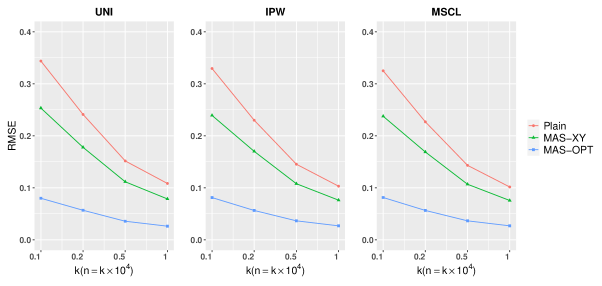
Figure 1: RMSE of different estimators under the logistic model with $N=10^{6}$ and $n=k\times 10^{4}$. Plain: subsampling estimator without integrating sample moments; MAS-XY: moment-assisted subsampling estimator with $\bm{h}(\bm{x},y)=\bm{x}y$; MAS-OPT: moment-assisted subsampling estimator with $\bm{h}(\bm{x},y)=\check{\bm{h}}^{\rm opt}(\bm{x},y)$.

Figure 1 shows that the moment-assisted subsampling estimators outperform the corresponding plain estimators for all three subsampling methods and all subsample sizes in terms of RMSE. This phenomenon is consistent with our theory that the estimation efficiency of subsampling methods can be improved by incorporating whole data sample moments. In addition, it can be seen that the moment-assisted estimators with $\bm{h}(\bm{x},y)=\check{\bm{h}}^{\rm opt}(\bm{x},y)$ have significantly smaller RMSEs than the moment-assisted estimators with $\bm{h}(\bm{x},y)=\bm{x}y$, which demonstrates the superiority of the optimal whole data sample moment.

We further calculated the bias and Monte Carlo standard deviation (MSD) of the above nine estimators. Due to space limitation, only the results of $n=2000$ and $n=10000$ are presented here for illustration, as shown in Table 1.

Table 1: Bias and MSD of different estimators for the $j$-th dimension of $\text{\boldmath{$\theta$}}_{0}$ under the logistic model with $N=10^{6}$. Plain: subsampling estimator without integrating sample moments; MAS-XY: moment-assisted subsampling estimator with $\bm{h}(\bm{x},y)=\bm{x}y$; MAS-OPT: moment-assisted subsampling estimator with $\bm{h}(\bm{x},y)=\check{\bm{h}}^{\rm opt}(\bm{x},y)$. The numbers in the Table are the results multiplied by 10.

$j$	UNI						IPW						MSCL
	Plain		MAS-XY		MAS-OPT		Plain		MAS-XY		MAS-OPT		Plain		MAS-XY		MAS-OPT
	Bias	MSD	Bias	MSD	Bias	MSD	Bias	MSD	Bias	MSD	Bias	MSD	Bias	MSD	Bias	MSD	Bias	MSD
$n=2000$
1	0.00	0.46	0.00	0.46	0.00	0.10	0.00	0.43	0.01	0.43	0.00	0.10	0.00	0.43	0.00	0.42	0.00	0.10
2	-0.03	0.77	0.00	0.56	-0.01	0.19	0.00	0.77	0.01	0.56	0.01	0.19	-0.01	0.76	0.00	0.55	0.01	0.19
3	-0.03	0.79	0.02	0.56	-0.01	0.19	0.00	0.75	0.02	0.53	0.00	0.18	0.00	0.74	0.02	0.52	0.00	0.18
4	0.01	0.79	0.00	0.57	0.00	0.19	0.00	0.76	0.01	0.55	0.00	0.19	-0.01	0.75	0.00	0.54	0.00	0.19
5	0.05	0.75	0.04	0.57	0.00	0.18	-0.01	0.74	0.01	0.54	0.00	0.18	0.00	0.73	0.01	0.54	0.00	0.18
6	-0.01	0.80	0.02	0.58	-0.02	0.19	-0.02	0.74	0.00	0.54	0.00	0.18	-0.02	0.73	0.00	0.53	0.00	0.18
7	0.01	0.79	0.02	0.57	0.00	0.18	0.01	0.74	0.02	0.54	0.00	0.19	0.01	0.73	0.02	0.54	0.00	0.19
8	0.01	0.82	0.00	0.58	-0.01	0.19	0.00	0.76	-0.01	0.58	0.01	0.18	0.00	0.74	-0.01	0.57	0.01	0.18
9	-0.02	0.79	-0.01	0.58	-0.01	0.18	-0.03	0.75	0.01	0.56	0.00	0.19	-0.03	0.74	0.01	0.55	0.00	0.19
10	0.03	0.79	0.03	0.58	0.00	0.19	-0.05	0.76	-0.02	0.55	-0.01	0.19	-0.05	0.76	-0.02	0.55	-0.01	0.19
$n=10000$
1	0.01	0.20	0.01	0.20	0.00	0.05	0.00	0.19	0.00	0.19	0.00	0.05	0.00	0.19	0.00	0.18	0.00	0.05
2	-0.01	0.34	0.00	0.24	0.00	0.08	0.00	0.34	0.00	0.24	0.00	0.09	0.00	0.33	0.00	0.24	0.00	0.09
3	0.00	0.35	0.00	0.25	0.00	0.09	0.00	0.36	0.01	0.25	0.00	0.08	0.00	0.35	0.01	0.25	0.00	0.08
4	0.01	0.35	0.00	0.26	0.00	0.09	0.01	0.35	0.01	0.24	0.00	0.09	0.01	0.34	0.01	0.24	0.00	0.09
5	0.00	0.36	0.01	0.26	0.00	0.08	-0.02	0.33	-0.01	0.24	0.00	0.09	-0.01	0.32	-0.01	0.24	0.00	0.09
6	0.00	0.35	0.01	0.25	0.00	0.09	0.00	0.33	0.01	0.25	0.00	0.09	0.00	0.33	0.01	0.25	0.00	0.09
7	0.00	0.35	0.00	0.25	0.00	0.08	-0.01	0.32	0.00	0.24	0.00	0.08	0.00	0.32	0.00	0.24	0.00	0.08
8	-0.01	0.36	-0.01	0.25	0.00	0.09	0.01	0.34	0.00	0.25	0.00	0.09	0.00	0.34	0.00	0.25	0.00	0.09
9	-0.01	0.36	-0.01	0.26	0.00	0.09	-0.02	0.34	0.00	0.25	0.00	0.09	-0.02	0.33	0.00	0.24	0.00	0.09
10	0.01	0.36	0.01	0.25	0.00	0.09	0.00	0.34	0.00	0.25	0.00	0.09	0.00	0.33	0.00	0.25	0.00	0.09

Table 1 shows that all the nine subsampling estimators have small biases for each dimension of the parameter, and the SDs decrease as the subsample size increases. The plain IPW and MSCL estimators perform better than the plain UNI estimator in terms of SD. However, the reduction of SD brought by the nonuniform subsampling probability is not substantial. In contrast, the moment-assisted subsampling estimators have far smaller SD than the corresponding plain estimators, especially when $\bm{h}(\bm{x},y)=\check{\bm{h}}^{\rm opt}(\bm{x},y)$.

Next, we evaluate the computational performance of the proposed estimators. We compare the CPU times of the above subsampling estimators and the whole data-based estimator. All calculations are implemented in the R programming (Team, 2016). The computer platform on which calculations are performed is a Windows server with a 24-core processor and 128GB RAM. Table 2 presents the CPU times under the logistic model.

Table 2: CPU times (second) of different estimators under the logistic model with $N=10^{6}$ and $n=k\times 10^{4}$.

$k$	UNI			IPW			MSCL
	Plain	MAS-XY	MAS-OPT	Plain	MAS-XY	MAS-OPT	Plain	MAS-XY	MAS-OPT
0.1	0.17	0.70	1.06	1.89	2.26	2.67	2.07	2.46	2.90
0.2	0.23	0.71	1.09	1.87	2.24	2.64	2.16	2.53	2.97
0.5	0.45	0.97	1.31	2.01	2.38	2.76	2.64	2.99	3.39
1	0.64	1.14	1.47	2.05	2.41	2.79	3.04	3.41	3.78
Whole-data based estimator: 123.63

From Table 2, it can be seen that the computing times of all nine subsampling estimators are significantly shorter than that of the whole data-based estimator. The computing times of the moment-assisted estimators are close to that of the corresponding plain estimators. This together with the results in Figure 1 and Table 1 shows that the proposed MAS strategy can significantly improve the estimation efficiency of the subsampling estimator with a little extra computational burden.

We consider the logistic model in this section, while similar results can be observed under other models. Further simulation results under the Weibull model can be found in Appendix D.

4 Real Data Application

In this section, we apply the MAS method to analyze the primary factors that affect aircraft delays using the large-scale flight data Airline on-time performance, which contains nearly 120 million records and takes up 1.6 GB of compressed space and 12 GB when uncompressed. The data includes flight arrival and departure details for all commercial flights within the United States from October 1987 through April 2008, and it is available at http://stat-computing.org/dataexpo/2009/the-data.html. We simply delete the records with missing variables without adjustment since the missing rate is low (no more than $2.5\%$), and then the resulting whole data size is $N=116,212,331$. The Federal Aviation Administration states that a flight is considered delay if it is fifteen minutes later than scheduled. Therefore we use the delay indicator ($1$: if the arrival delay is fifteen minutes or more; $0$: otherwise) as response $Y$ and build a logistic model to describe the relationship between the delay indicator and the following six variables: day/night ($X_{1}$, $1$: if the departure time is between $7$am and $6$pm; $0$: otherwise), weekend/weekday ($X_{2}$, $1$: if departure occurred in the weekend; $0$: otherwise), the departure delay ($X_{3}$, $1$: if departure delay is 15 minutes or more; $0$: otherwise), and pairwise interaction terms of the three variables ($X_{1}X_{2}$, $X_{1}X_{3}$, $X_{2}X_{3}$). We denote $\text{\boldmath{$X$}}=(X_{1},X_{2},X_{3},X_{1}X_{2},X_{1}X_{3},X_{2}X_{3})$ as a $6$-dimensional vector of covariates. Then the logistic model has the form

$$P(Y=1\mid\text{\boldmath{$X$}}=\bm{x})=\frac{\exp(\alpha_{0}+\bm{x}^{{\mathrm{\scriptscriptstyle T}}}\bm{\beta}_{0})}{1+\exp(\alpha_{0}+\bm{x}^{{\mathrm{\scriptscriptstyle T}}}\bm{\beta}_{0})},$$

where $\text{\boldmath{$\theta$}}_{0}=(\alpha_{0},\bm{\beta}_{0})$ is the parameter of interest.

In practice, many researchers do not possess powerful computational resources, e.g., server clusters or distributional systems. Therefore, it is important to provide an estimator that can be carried out on handy computational resources. For the considered data set, the whole data-based estimator of $\text{\boldmath{$\theta$}}_{0}$ is computationally infeasible for many commonly available devices such as laptops and personal computers. To mimic the situation with limited computational resources, we conducted the analysis on a laptop with a 4-core processor and 16GB RAM. The program runs out of memory when implementing the whole data-based estimator on the laptop. The subsampling strategy can be adopted to tackle the problem. We apply the proposed method to estimate $\text{\boldmath{$\theta$}}_{0}$. For comparison, we calculate the nine subsampling estimators listed at the beginning of Section 3. We take the subsample size $n$ to be $50000$. In addition, a pilot subsample of size $2000$ is drawn to calculate the nonuniform subsampling probability and $\check{\bm{h}}^{\rm opt}(\bm{x},y)$. Table 3 presents the estimation results and the estimated SD. The estimated SDs are close to the Mote Carlo SDs for the nine subsampling estimators, which have been illustrated in Appendix D. In addition, Table 4 presents the CPU times of the nine subsampling estimators.

Table 3: Estimation (Est) and estimated standard deviation (ESD) of subsampling estimators for the $j$-th dimension of $\text{\boldmath{$\theta$}}_{0}$ in the airline data with $N=116,212,331$ and $n=50000$. The numbers of ESD in the Table are the results multiplied by 10.

$j$	UNI						IPW						MSCL
	Plain		MAS-XY		MAS-OPT		Plain		MAS-XY		MAS-OPT		Plain		MAS-XY		MAS-OPT
	Est	ESD	Est	ESD	Est	ESD	Est	ESD	Est	ESD	Est	ESD	Est	ESD	Est	ESD	Est	ESD
1	-2.76	0.68	-2.76	0.68	-2.73	0.04	-2.73	0.22	-2.73	0.21	-2.72	0.03	-2.73	0.21	-2.73	0.21	-2.72	0.03
2	0.15	0.76	0.14	0.67	0.12	0.05	0.12	0.29	0.13	0.23	0.12	0.03	0.12	0.29	0.13	0.23	0.12	0.03
3	0.26	0.75	0.26	0.67	0.24	0.05	0.25	0.30	0.26	0.23	0.24	0.04	0.25	0.28	0.26	0.23	0.24	0.04
4	4.35	0.88	4.43	0.83	4.38	0.09	4.40	0.37	4.39	0.30	4.40	0.07	4.40	0.35	4.40	0.30	4.40	0.07
5	-0.07	0.82	-0.01	0.71	-0.02	0.06	-0.05	0.37	-0.05	0.29	-0.01	0.04	-0.05	0.37	-0.05	0.29	-0.01	0.04
6	-0.44	0.78	-0.47	0.67	-0.44	0.10	-0.46	0.39	-0.44	0.27	-0.46	0.08	-0.46	0.38	-0.45	0.27	-0.46	0.08
7	0.09	0.82	0.03	0.71	0.03	0.06	0.04	0.39	0.02	0.29	0.03	0.05	0.04	0.38	0.02	0.29	0.03	0.05

Table 4: CPU times (second) of different estimators in the airline data with $N=116,212,331$ and $n=50000$.

UNI			IPW			MSCL
Plain	MAS-XY	MAS-OPT	Plain	MAS-XY	MAS-OPT	Plain	MAS-XY	MAS-OPT
32.11	33.53	76.21	90.81	93.02	109.12	92.75	95.00	111.12

As shown in Table 3, the estimated coefficients given by the nine subsampling estimators are similar to each other and come to the same conclusion that $X_{1}$, $X_{2}$, $X_{3}$ and the interaction terms $X_{2}X_{3}$ have positive effects and the interaction terms $X_{1}X_{2}$ and $X_{1}X_{3}$ have negative effects on the aircraft delay. However, the moment-assisted subsampling estimators have smaller estimated standard deviations than the plain subsampling estimators in all coefficient estimates. According to the numerical results in Appendix D, the estimated standard deviations are very close to the true standard deviations. Table 4 shows that the subsampling methods can be implemented quickly. The plain UNI estimator takes the shortest computing time, but its efficiency is notably lower than other estimators. The computing times of the moment-assisted estimators with $\bm{h}(\bm{x},y)=\bm{x}y$ are very close to those of the corresponding plain estimators. The computing times of the moment-assisted estimators with $\bm{h}(\bm{x},y)=\check{\bm{h}}^{\rm opt}(\bm{x},y)$ are slightly longer than those of the corresponding plain estimators. Such an increase in computing time is acceptable, given the substantial efficiency improvement of the moment-assisted method. Additional results and discussion of the proposed method can be found in Appendix D.

In Appendices A–C, we provide proofs and technical details of the theoretical results in the main text. Throughout the proof, let $A_{ij}$ denote the $i$-th row and $j$-th column element of the generic matrix $\mathbf{A}$ and let $c$ be a generic positive constant that may be different in different places. Further numerical results can be found in in Appendix D.

Appendix A Proof of Theorem 1

Recalling the definition of $\tilde{\bm{g}}(\text{\boldmath{$\theta$}})$ and by Taylor’s expansion, we have $\tilde{g}(\tilde{\text{\boldmath{$\theta$}}})=\tilde{g}(\text{\boldmath{$\theta$}}_{0})+\bar{\mathbf{G}}(\tilde{\text{\boldmath{$\theta$}}}-\text{\boldmath{$\theta$}}_{0})$, where $\bar{\mathbf{G}}=\partial\tilde{\bm{g}}(\text{\boldmath{$\theta$}})/\partial\text{\boldmath{$\theta$}}\mid_{\text{\boldmath{$\theta$}}=\bar{\text{\boldmath{$\theta$}}}}$ and $\bar{\text{\boldmath{$\theta$}}}$ is between $\text{\boldmath{$\theta$}}_{0}$ and $\tilde{\text{\boldmath{$\theta$}}}$. By the definition of $\tilde{\text{\boldmath{$\theta$}}}_{\rm MAS}$ and straightforward algebras, we have

$$\begin{split}&n^{1/2}\mathbf{V}_{\bm{h}}^{-1/2}(\tilde{\text{\boldmath{$\theta$}}}_{\rm MAS}-\text{\boldmath{$\theta$}}_{0})\\ &=-n^{1/2}\mathbf{V}_{\bm{h}}^{-1/2}\left(\mathbf{G}^{{\mathrm{\scriptscriptstyle T}}}\mathbf{\Omega}^{-1}\mathbf{G}\right)^{-1}\mathbf{G}^{{\mathrm{\scriptscriptstyle T}}}\mathbf{\Omega}^{-1}\tilde{\bm{g}}(\text{\boldmath{$\theta$}}_{0})\\ &\quad+n^{1/2}\mathbf{V}_{\bm{h}}^{-1/2}\left(\mathbf{G}^{{\mathrm{\scriptscriptstyle T}}}\mathbf{\Omega}^{-1}\mathbf{G}\right)^{-1}\mathbf{G}^{{\mathrm{\scriptscriptstyle T}}}\mathbf{\Omega}^{-1}\left(\widetilde{\mathbf{G}}-\bar{\mathbf{G}}\right)(\tilde{\text{\boldmath{$\theta$}}}-\text{\boldmath{$\theta$}}_{0})\\ &\quad+n^{1/2}\mathbf{V}_{\bm{h}}^{-1/2}\left(\left(\widetilde{\mathbf{G}}^{{\mathrm{\scriptscriptstyle T}}}\widetilde{\mathbf{\Omega}}^{-1}\widetilde{\mathbf{G}}\right)^{-1}\widetilde{\mathbf{G}}^{{\mathrm{\scriptscriptstyle T}}}\widetilde{\mathbf{\Omega}}^{-1}-\left(\mathbf{G}^{{\mathrm{\scriptscriptstyle T}}}\mathbf{\Omega}^{-1}\mathbf{G}\right)^{-1}\mathbf{G}^{{\mathrm{\scriptscriptstyle T}}}\mathbf{\Omega}^{-1}\right)\left(\widetilde{\mathbf{G}}-\bar{\mathbf{G}}\right)(\tilde{\text{\boldmath{$\theta$}}}-\text{\boldmath{$\theta$}}_{0})\\ &\quad-n^{1/2}\mathbf{V}_{\bm{h}}^{-1/2}\left(\left(\widetilde{\mathbf{G}}^{{\mathrm{\scriptscriptstyle T}}}\widetilde{\mathbf{\Omega}}^{-1}\widetilde{\mathbf{G}}\right)^{-1}\widetilde{\mathbf{G}}^{{\mathrm{\scriptscriptstyle T}}}\widetilde{\mathbf{\Omega}}^{-1}-\left(\mathbf{G}^{{\mathrm{\scriptscriptstyle T}}}\mathbf{\Omega}^{-1}\mathbf{G}\right)^{-1}\mathbf{G}^{{\mathrm{\scriptscriptstyle T}}}\mathbf{\Omega}^{-1}\right)\tilde{\bm{g}}(\text{\boldmath{$\theta$}}_{0})\\ &\triangleq U_{1}+U_{2}+U_{3}+U_{4}.\end{split}$$

To prove the asymptotic normality in Theorem 1, it suffices to prove $U_{1}\stackrel{{\scriptstyle d}}{{\to}}N(0,\mathbf{I})$ and $U_{i}=o_{P}(1)$ for $i=2,3,4$.

We first prove $U_{1}\stackrel{{\scriptstyle d}}{{\to}}N(0,\mathbf{I})$. By the definition of $\tilde{\bm{g}}(\text{\boldmath{$\theta$}}_{0})$, it is easy to observe that

$$n^{1/2}\mathbf{V}_{\bm{h}}^{-1/2}(\mathbf{G}^{{\mathrm{\scriptscriptstyle T}}}\mathbf{\Omega}^{-1}\mathbf{G})^{-1}\mathbf{G}^{{\mathrm{\scriptscriptstyle T}}}\mathbf{\Omega}^{-1}\tilde{\bm{g}}(\text{\boldmath{$\theta$}}_{0})$$

$$=n^{1/2}\mathbf{V}_{\bm{h}}^{-1/2}(\mathbf{G}^{{\mathrm{\scriptscriptstyle T}}}\mathbf{\Omega}^{-1}\mathbf{G})^{-1}\mathbf{G}^{{\mathrm{\scriptscriptstyle T}}}\mathbf{\Omega}^{-1}\sum_{i=1}^{N}\begin{pmatrix}n^{-1}\delta_{i}\bm{u}(\text{\boldmath{$X$}}_{i},Y_{i};\text{\boldmath{$\theta$}})\\ n^{-1}\delta_{i}\bm{v}(\text{\boldmath{$X$}}_{i};\text{\boldmath{$\theta$}},\bm{\mu}_{0})-N^{-1}\left(\bm{h}(\text{\boldmath{$X$}}_{i},Y_{i})-\bm{\mu}_{0}\right)\end{pmatrix}$$

$$\quad-n^{1/2}\mathbf{V}_{\bm{h}}^{-1/2}(\mathbf{G}^{{\mathrm{\scriptscriptstyle T}}}\mathbf{\Omega}^{-1}\mathbf{G})^{-1}\mathbf{G}^{{\mathrm{\scriptscriptstyle T}}}\mathbf{\Omega}^{-1}\begin{pmatrix}0\\ \left(N^{-1}\sum_{i=1}^{N}\delta_{i}p(\text{\boldmath{$X$}}_{i},Y_{i})^{-1}-1\right)(\hat{\bm{\mu}}-\bm{\mu}_{0})\end{pmatrix}.$$

Note that $E[N^{-1}\sum_{i=1}^{N}\delta_{i}p(\text{\boldmath{$X$}}_{i},Y_{i})^{-1}-1]=0$. In addition, by Condition (C4),

$${\rm var}\left(N^{-1}\sum_{i=1}^{N}\delta_{i}p(\text{\boldmath{$X$}}_{i},Y_{i})^{-1}\right)\leq N^{-1}E[p(\text{\boldmath{$X$}},Y)^{-1}]=O(n^{-1}).$$

By Chebyshev’s inequality, we have $N^{-1}\sum_{i=1}^{N}\delta_{i}p(\text{\boldmath{$X$}}_{i},Y_{i})^{-1}-1=O_{P}(n^{-1/2})$. By the definition of $\hat{\bm{\mu}}$ and Condition (C2)(i), we have $\|\hat{\bm{\mu}}-\bm{\mu}_{0}\|=O_{P}(N^{-1/2})$. By the definition of $\mathbf{V}_{\bm{h}}$, we have

$$\|n^{1/2}\mathbf{V}_{\bm{h}}^{-1/2}(\mathbf{G}^{{\mathrm{\scriptscriptstyle T}}}\mathbf{\Omega}^{-1}\mathbf{G})^{-1}\mathbf{G}^{{\mathrm{\scriptscriptstyle T}}}\mathbf{\Omega}^{-1}\|\leq n^{1/2}\|(\mathbf{G}^{{\mathrm{\scriptscriptstyle T}}}\mathbf{\Omega}^{-1}\mathbf{G})^{-1/2}\mathbf{G}^{{\mathrm{\scriptscriptstyle T}}}\mathbf{\Omega}^{-1/2}\|\|\mathbf{\Omega}^{-1/2}\|=O(n^{1/2}\lambda_{\min,\mathbf{\Omega}}^{-1/2}).$$

Combing these results and the condition $n^{1/2}\lambda_{\rm min,\mathbf{\Omega}}\to\infty$ in Condition (C5), we have

$$\|n^{1/2}\mathbf{V}_{\bm{h}}^{-1/2}(\mathbf{G}^{{\mathrm{\scriptscriptstyle T}}}\mathbf{\Omega}^{-1}\mathbf{G})^{-1}\mathbf{G}^{{\mathrm{\scriptscriptstyle T}}}\mathbf{\Omega}^{-1}\|\Big{|}N^{-1}\sum_{i=1}^{N}\delta_{i}p(\text{\boldmath{$X$}}_{i},Y_{i})^{-1}-1\Big{|}\|\hat{\bm{\mu}}-\bm{\mu}_{0}\|=o_{P}(1)$$

and hence

$$n^{1/2}\mathbf{V}_{\bm{h}}^{-1/2}(\mathbf{G}^{{\mathrm{\scriptscriptstyle T}}}\mathbf{\Omega}^{-1}\mathbf{G})^{-1}\mathbf{G}^{{\mathrm{\scriptscriptstyle T}}}\mathbf{\Omega}^{-1}\tilde{\bm{g}}(\text{\boldmath{$\theta$}}_{0})=\sum_{i=1}^{N}K_{i}+o_{P}(1),$$

where

$$K_{i}=n^{1/2}\mathbf{V}_{\bm{h}}^{-1/2}(\mathbf{G}^{{\mathrm{\scriptscriptstyle T}}}\mathbf{\Omega}^{-1}\mathbf{G})^{-1}\mathbf{G}^{{\mathrm{\scriptscriptstyle T}}}\mathbf{\Omega}^{-1}\begin{pmatrix}n^{-1}\delta_{i}\bm{u}(\text{\boldmath{$X$}}_{i},Y_{i};\text{\boldmath{$\theta$}}_{0})\\ n^{-1}\delta_{i}\bm{v}(\text{\boldmath{$X$}}_{i};\text{\boldmath{$\theta$}}_{0},\bm{\mu}_{0})-N^{-1}\left(\bm{h}(\text{\boldmath{$X$}}_{i},Y_{i})-\bm{\mu}_{0}\right)\end{pmatrix}.$$

To prove $U_{1}\stackrel{{\scriptstyle d}}{{\to}}N(0,\mathbf{I})$, it suffices to prove $\sum_{i=1}^{N}K_{i}\stackrel{{\scriptstyle d}}{{\to}}N(0,\mathbf{I})$. It is easy to verify that $\sum_{i=1}^{N}{\rm cov}(K_{i})\to\mathbf{I}$. By Lindeberg-Feller central limit theorem in van der Vaart (2000), to prove $\sum_{i=1}^{N}K_{i}\stackrel{{\scriptstyle d}}{{\to}}N(0,\mathbf{I})$, it suffices to verify that for any given $\epsilon>0$,

$$\sum_{i=1}^{N}E[\|K_{i}\|^{2}1(\|K_{i}\|>\epsilon)]\to 0,$$

where $1(\cdot)$ is an indicator function. Since for any given $\tau>0$, we have $E[\|K_{1}\|^{2}1(\|K_{1}\|>\epsilon)]\leq E[\|K_{1}\|^{2+\tau}/\epsilon^{\tau}]$. Then it suffices to prove that $NE[\|K_{1}\|^{2+\tau}]=o(1)$ for some $\tau>0$. Let $B=n^{-1/2}\mathbf{V}_{\bm{h}}^{-1/2}(\mathbf{G}^{{\mathrm{\scriptscriptstyle T}}}\mathbf{\Omega}^{-1}\mathbf{G})^{-1}\mathbf{G}^{{\mathrm{\scriptscriptstyle T}}}\mathbf{\Omega}^{-1}$ and $\bm{b}_{j}^{{\mathrm{\scriptscriptstyle T}}}$ be the $j$-row of $B$ for $j=1,\dots,d$. Then we can rewrite $K_{1}=(\bm{b}_{1}^{{\mathrm{\scriptscriptstyle T}}}\bm{m}_{1},\dots,\bm{b}_{d}^{{\mathrm{\scriptscriptstyle T}}}\bm{m}_{1})^{{\mathrm{\scriptscriptstyle T}}}$ where $\bm{m}_{1}=(\delta_{1}\bm{u}(\text{\boldmath{$X$}}_{1},Y_{1};\text{\boldmath{$\theta$}}_{0})^{{\mathrm{\scriptscriptstyle T}}},\delta_{1}\bm{v}(\text{\boldmath{$X$}}_{1};\text{\boldmath{$\theta$}}_{0},\bm{\mu}_{0})^{{\mathrm{\scriptscriptstyle T}}}-\rho\left(\bm{h}(\text{\boldmath{$X$}}_{1},Y_{1})-\bm{\mu}_{0}\right)^{{\mathrm{\scriptscriptstyle T}}})^{{\mathrm{\scriptscriptstyle T}}}$. By the inequality $(t_{1}+t_{2})^{p}\leq 2^{p-1}(|t_{1}|^{p}+|t_{2}|^{p})$ and Condition (C3), we have

$$\begin{split}NE[\|K_{1}\|^{2+\tau}]&\leq cNE[|b_{1}^{{\mathrm{\scriptscriptstyle T}}}\bm{m}_{1}|^{2+\tau}+\dots+|b_{d}^{{\mathrm{\scriptscriptstyle T}}}\bm{m}_{1}|^{2+\tau}]\\ &\leq cN({\rm var}(b_{1}^{{\mathrm{\scriptscriptstyle T}}}\bm{m}_{1})^{1+\tau/2}+\dots+{\rm var}(b_{d}^{{\mathrm{\scriptscriptstyle T}}}\bm{m}_{1})^{1+\tau/2})\\ &=cN\|\left(\mathsf{diag}(E[K_{1}K_{1}^{{\mathrm{\scriptscriptstyle T}}}])\right)^{1+\tau/2}\|_{1},\end{split}$$

where $\|\cdot\|_{1}$ denotes the $1$-norm for a vector. Then it is proved that $NE[\|K_{1}\|^{2+\tau}]=o(1)$ since $E[K_{1}K_{1}^{{\mathrm{\scriptscriptstyle T}}}]=N^{-1}\mathbf{I}$.

Now it remains to prove $U_{i}=o_{P}(1)$ for $i=2,3,4$

We first prove $\|U_{2}\|=o_{P}(1)$. Note that

$$\|U_{2}\| \leq n^{1/2}\|\left(\mathbf{G}^{{\mathrm{\scriptscriptstyle T}}}\mathbf{\Omega}^{-1}\mathbf{G}\right)^{-1/2}\mathbf{G}^{{\mathrm{\scriptscriptstyle T}}}\mathbf{\Omega}^{-1/2}\|\|\mathbf{\Omega}^{-1/2}\|\|\widetilde{\mathbf{G}}-\bar{\mathbf{G}}\|\|\tilde{\text{\boldmath{$\theta$}}}-\text{\boldmath{$\theta$}}_{0}\|.$$

Lemma 1 behind this proof shows that $\widetilde{G}_{jl}-G_{jl}=O_{P}(n^{-1/2})$ and $\widetilde{\Omega}_{jk}-\Omega_{jk}=O_{P}(n^{-1/2})$ for $j,k=1,\dots,d+q$ and $l=1,\dots,d$. Then by the W-H theorem in Hoffman and Wielandt (1953), we have

$$\|\widetilde{\mathbf{G}}-\mathbf{G}\|=O_{P}(n^{-1/2})$$ (16)

and

$$\|\widetilde{\mathbf{\Omega}}-\mathbf{\Omega}\|=O_{P}(n^{-1/2}).$$ (17)

Similar techniques can be used to prove

$$\|\bar{\mathbf{G}}-\mathbf{G}\|=O_{P}(n^{-1/2})$$ (18)

and hence

$$\|\widetilde{\mathbf{G}}-\bar{\mathbf{G}}\|=O_{P}(n^{-1/2}).$$ (19)

In addition, we have

$$\|\left(\mathbf{G}^{{\mathrm{\scriptscriptstyle T}}}\mathbf{\Omega}^{-1}\mathbf{G}\right)^{-1/2}\mathbf{G}^{{\mathrm{\scriptscriptstyle T}}}\mathbf{\Omega}^{-1/2}\|=1$$ (20)

and $\|\mathbf{\Omega}^{-1/2}\|=\lambda_{\min,\mathbf{\Omega}}^{-1/2}$. Then by Condition (C6) and $n^{1/2}\lambda_{\min,\mathbf{\Omega}}\to\infty$ in Condition (C5), we have $\|U_{2}\|=O_{P}(n^{-1/2}\lambda_{\min,\mathbf{\Omega}}^{-1/2})=o_{P}(1)$.

For $U_{3}$ and $U_{4}$, by some algebras, we have

$$\begin{split}&n^{1/2}\mathbf{V}_{\bm{h}}^{-1/2}\left(\left(\widetilde{\mathbf{G}}^{{\mathrm{\scriptscriptstyle T}}}\widetilde{\mathbf{\Omega}}^{-1}\widetilde{\mathbf{G}}\right)^{-1}\widetilde{\mathbf{G}}^{{\mathrm{\scriptscriptstyle T}}}\widetilde{\mathbf{\Omega}}^{-1}-\left(\mathbf{G}^{{\mathrm{\scriptscriptstyle T}}}\mathbf{\Omega}^{-1}\mathbf{G}\right)^{-1}\mathbf{G}^{{\mathrm{\scriptscriptstyle T}}}\mathbf{\Omega}^{-1}\right)\\ &=n^{1/2}\left(\mathbf{G}^{{\mathrm{\scriptscriptstyle T}}}\mathbf{\Omega}^{-1}\mathbf{G}\right)^{-1/2}(\widetilde{\mathbf{G}}-\mathbf{G})^{{\mathrm{\scriptscriptstyle T}}}(\widetilde{\mathbf{\Omega}}^{-1}-\mathbf{\Omega}^{-1})\\ &\quad+n^{1/2}\left(\mathbf{G}^{{\mathrm{\scriptscriptstyle T}}}\mathbf{\Omega}^{-1}\mathbf{G}\right)^{-1/2}\mathbf{G}^{{\mathrm{\scriptscriptstyle T}}}\mathbf{\Omega}^{-1}(\mathbf{\Omega}-\widetilde{\mathbf{\Omega}})\widetilde{\mathbf{\Omega}}^{-1}\\ &\quad+n^{1/2}\left(\mathbf{G}^{{\mathrm{\scriptscriptstyle T}}}\mathbf{\Omega}^{-1}\mathbf{G}\right)^{-1/2}\left[\mathbf{G}^{{\mathrm{\scriptscriptstyle T}}}\mathbf{\Omega}^{-1}\mathbf{G}-\widetilde{\mathbf{G}}^{{\mathrm{\scriptscriptstyle T}}}\widetilde{\mathbf{\Omega}}^{-1}\widetilde{\mathbf{G}}\right]\left(\widetilde{\mathbf{G}}^{{\mathrm{\scriptscriptstyle T}}}\widetilde{\mathbf{\Omega}}^{-1}\widetilde{\mathbf{G}}\right)^{-1}\widetilde{\mathbf{G}}^{{\mathrm{\scriptscriptstyle T}}}\widetilde{\mathbf{\Omega}}^{-1}\\ &\quad+n^{1/2}\left(\mathbf{G}^{{\mathrm{\scriptscriptstyle T}}}\mathbf{\Omega}^{-1}\mathbf{G}\right)^{-1/2}(\widetilde{\mathbf{G}}-\mathbf{G})^{{\mathrm{\scriptscriptstyle T}}}\mathbf{\Omega}^{-1}\\ &\triangleq T_{1}+T_{2}+T_{3}+T_{4}.\end{split}$$ (21)

To prove $U_{3}=o_{P}(1)$, it suffices to prove

$$\|T_{i}(\widetilde{\mathbf{G}}-\bar{\mathbf{G}})(\tilde{\text{\boldmath{$\theta$}}}-\text{\boldmath{$\theta$}}_{0})\|=o_{P}(1),\quad{\rm for}\quad i=1,2,3,4$$

Note that

$$\|T_{1}(\widetilde{\mathbf{G}}-\bar{\mathbf{G}})(\tilde{\text{\boldmath{$\theta$}}}-\text{\boldmath{$\theta$}}_{0})\|$$

$$\leq n^{1/2}\|\left(\mathbf{G}^{{\mathrm{\scriptscriptstyle T}}}\mathbf{\Omega}^{-1}\mathbf{G}\right)^{-1/2}\|\|\widetilde{\mathbf{G}}-\mathbf{G}\|\|\mathbf{\Omega}^{-1}\|\|\widetilde{\mathbf{\Omega}}-\mathbf{\Omega}\|\|\widetilde{\mathbf{\Omega}}^{-1}\|\|\widetilde{\mathbf{G}}-\bar{\mathbf{G}}\|\|\tilde{\text{\boldmath{$\theta$}}}-\text{\boldmath{$\theta$}}_{0}\|.$$

By Condition (C5), we have

$$\|\left(\mathbf{G}^{{\mathrm{\scriptscriptstyle T}}}\mathbf{\Omega}^{-1}\mathbf{G}\right)^{-1/2}\|=O(1).$$ (22)

Denote $\lambda_{\min,\widetilde{\mathbf{\Omega}}}$ as the minimum eigenvalue of $\widetilde{\mathbf{\Omega}}$. By Lemma 1 and the W-H theorem in Hoffman and Wielandt (1953), we have

$$\lambda_{\min,\widetilde{\mathbf{\Omega}}}=\lambda_{\min,\mathbf{\Omega}}+O_{P}(n^{-1/2})=\lambda_{\min,\mathbf{\Omega}}(1+O_{P}(\lambda_{\min,\mathbf{\Omega}}^{-1}n^{-1/2}))=\lambda_{\min,\mathbf{\Omega}}(1+o_{P}(1))$$ (23)

Then we have

$$\|\widetilde{\mathbf{\Omega}}^{-1}\|=\lambda_{\min,\widetilde{\mathbf{\Omega}}}^{-1}=\lambda_{\min,\mathbf{\Omega}}^{-1}(1+o_{P}(1)).$$ (24)

These results together with (16), (17), (19), and Condition (C6) prove

$$\|T_{1}(\widetilde{\mathbf{G}}-\bar{\mathbf{G}})^{{\mathrm{\scriptscriptstyle T}}}(\tilde{\text{\boldmath{$\theta$}}}-\text{\boldmath{$\theta$}}_{0})\|=O_{P}(\lambda_{\min,\mathbf{\Omega}}^{-2}n^{-3/2})=o_{P}(1).$$ (25)

Further, note that

$$\|T_{2}(\widetilde{\mathbf{G}}-\bar{\mathbf{G}})(\tilde{\text{\boldmath{$\theta$}}}-\text{\boldmath{$\theta$}}_{0})\|$$

$$\leq n^{1/2}\|\left(\mathbf{G}^{{\mathrm{\scriptscriptstyle T}}}\mathbf{\Omega}^{-1}\mathbf{G}\right)^{-1/2}\mathbf{G}\mathbf{\Omega}^{-1/2}\|\|\mathbf{\Omega}^{-1/2}(\mathbf{\Omega}-\widetilde{\mathbf{\Omega}})\widetilde{\mathbf{\Omega}}^{-1/2}\|\|\widetilde{\mathbf{\Omega}}^{-1/2}\|\|\widetilde{\mathbf{G}}-\bar{\mathbf{G}}\|\|\tilde{\text{\boldmath{$\theta$}}}-\text{\boldmath{$\theta$}}_{0}\|$$

and

$$\|T_{4}(\widetilde{\mathbf{G}}-\bar{\mathbf{G}})(\tilde{\text{\boldmath{$\theta$}}}-\text{\boldmath{$\theta$}}_{0})\| \leq n^{1/2}\|\left(\mathbf{G}^{{\mathrm{\scriptscriptstyle T}}}\mathbf{\Omega}^{-1}\mathbf{G}\right)^{-1/2}\|\|\widetilde{\mathbf{G}}-\mathbf{G}\|\|\|\mathbf{\Omega}^{-1}\|\|\widetilde{\mathbf{G}}-\bar{\mathbf{G}}\|\|\tilde{\text{\boldmath{$\theta$}}}-\text{\boldmath{$\theta$}}_{0}\|.$$

By (23), we have

$$\|\widetilde{\mathbf{\Omega}}^{-1/2}\|=\lambda_{\min,\widetilde{\mathbf{\Omega}}}^{-1/2}=\lambda_{\min,\mathbf{\Omega}}^{-1/2}(1+o_{P}(1)).$$ (26)

In addition, by (17) and Condition (C5), we have

$$\|\mathbf{\Omega}^{-1/2}(\mathbf{\Omega}-\widetilde{\mathbf{\Omega}})\widetilde{\mathbf{\Omega}}^{-1/2}\|\leq\|\mathbf{\Omega}^{-1/2}\|\|\mathbf{\Omega}-\widetilde{\mathbf{\Omega}}\|\|\widetilde{\mathbf{\Omega}}^{-1/2}\|=O_{P}(\lambda_{\min,\mathbf{\Omega}}^{-1}n^{-1/2})$$ (27)

These together with (16), (20), (22), (24), (26), (19), and Condition (C6) prove

$$\|T_{2}(\widetilde{\mathbf{G}}-\bar{\mathbf{G}})(\tilde{\text{\boldmath{$\theta$}}}-\text{\boldmath{$\theta$}}_{0})\|=O_{P}(\lambda_{\min,\mathbf{\Omega}}^{-3/2}n^{-1})=o_{P}(1)$$ (28)

and

$$\|T_{4}(\widetilde{\mathbf{G}}-\bar{\mathbf{G}})(\tilde{\text{\boldmath{$\theta$}}}-\text{\boldmath{$\theta$}}_{0})\|=O_{P}(\lambda_{\min,\mathbf{\Omega}}^{-1}n^{-1})=o_{P}(1).$$ (29)

Now to prove $U_{3}=o_{P}(1)$, it remains to prove $\|T_{3}(\widetilde{\mathbf{G}}-\bar{\mathbf{G}})(\tilde{\text{\boldmath{$\theta$}}}-\text{\boldmath{$\theta$}}_{0})\|=o_{P}(1)$. Note that

$$\begin{split}&\widetilde{\mathbf{G}}^{{\mathrm{\scriptscriptstyle T}}}\widetilde{\mathbf{\Omega}}^{-1}\widetilde{\mathbf{G}}-\mathbf{G}^{{\mathrm{\scriptscriptstyle T}}}\mathbf{\Omega}^{-1}\mathbf{G}\\ &=\left\{(\widetilde{\mathbf{G}}-\mathbf{G})^{{\mathrm{\scriptscriptstyle T}}}\mathbf{\Omega}^{-1}(\widetilde{\mathbf{G}}-\mathbf{G})+\mathbf{G}^{{\mathrm{\scriptscriptstyle T}}}\mathbf{\Omega}^{-1}(\widetilde{\mathbf{G}}-\mathbf{G})+(\widetilde{\mathbf{G}}-\mathbf{G})^{{\mathrm{\scriptscriptstyle T}}}\mathbf{\Omega}^{-1}\mathbf{G}+(\widetilde{\mathbf{G}}-\mathbf{G})^{{\mathrm{\scriptscriptstyle T}}}(\widetilde{\mathbf{\Omega}}^{-1}-\mathbf{\Omega}^{-1})\widetilde{\mathbf{G}}\right\}\\ &\quad+\mathbf{G}^{{\mathrm{\scriptscriptstyle T}}}\mathbf{\Omega}^{-1}(\mathbf{\Omega}-\widetilde{\mathbf{\Omega}})\widetilde{\mathbf{\Omega}}^{-1}\widetilde{\mathbf{G}}\\ &\triangleq W+\mathbf{G}^{{\mathrm{\scriptscriptstyle T}}}\mathbf{\Omega}^{-1}(\mathbf{\Omega}-\widetilde{\mathbf{\Omega}})\widetilde{\mathbf{\Omega}}^{-1}\widetilde{\mathbf{G}}.\end{split}$$

Then we have

$$\|T_{3}(\widetilde{\mathbf{G}}-\bar{\mathbf{G}})^{{\mathrm{\scriptscriptstyle T}}}(\tilde{\text{\boldmath{$\theta$}}}-\text{\boldmath{$\theta$}}_{0})\|$$

$$\leq n^{1/2}\|\left(\mathbf{G}^{{\mathrm{\scriptscriptstyle T}}}\mathbf{\Omega}^{-1}\mathbf{G}\right)^{-1/2}W\left(\widetilde{\mathbf{G}}^{{\mathrm{\scriptscriptstyle T}}}\widetilde{\mathbf{\Omega}}^{-1}\widetilde{\mathbf{G}}\right)^{-1}\widetilde{\mathbf{G}}^{{\mathrm{\scriptscriptstyle T}}}\widetilde{\mathbf{\Omega}}^{-1}(\widetilde{\mathbf{G}}-\bar{\mathbf{G}})(\tilde{\text{\boldmath{$\theta$}}}-\text{\boldmath{$\theta$}}_{0})\|$$

$$\quad+n^{1/2}\|\left(\mathbf{G}^{{\mathrm{\scriptscriptstyle T}}}\mathbf{\Omega}^{-1}\mathbf{G}\right)^{-1/2}\mathbf{G}^{{\mathrm{\scriptscriptstyle T}}}\mathbf{\Omega}^{-1}(\mathbf{\Omega}-\widetilde{\mathbf{\Omega}})\widetilde{\mathbf{\Omega}}^{-1}\widetilde{\mathbf{G}}\left(\widetilde{\mathbf{G}}^{{\mathrm{\scriptscriptstyle T}}}\widetilde{\mathbf{\Omega}}^{-1}\widetilde{\mathbf{G}}\right)^{-1}\widetilde{\mathbf{G}}^{{\mathrm{\scriptscriptstyle T}}}\widetilde{\mathbf{\Omega}}^{-1}(\widetilde{\mathbf{G}}-\bar{\mathbf{G}})(\tilde{\text{\boldmath{$\theta$}}}-\text{\boldmath{$\theta$}}_{0})\|$$

$$\leq n^{1/2}\|\left(\mathbf{G}^{{\mathrm{\scriptscriptstyle T}}}\mathbf{\Omega}^{-1}\mathbf{G}\right)^{-1/2}\|\|W\|\|\left(\widetilde{\mathbf{G}}^{{\mathrm{\scriptscriptstyle T}}}\widetilde{\mathbf{\Omega}}^{-1}\widetilde{\mathbf{G}}\right)^{-1}\widetilde{\mathbf{G}}^{{\mathrm{\scriptscriptstyle T}}}\widetilde{\mathbf{\Omega}}^{-1/2}\|\|\widetilde{\mathbf{\Omega}}^{-1/2}\|\|\widetilde{\mathbf{G}}-\bar{\mathbf{G}}\|\|\tilde{\text{\boldmath{$\theta$}}}-\text{\boldmath{$\theta$}}_{0}\|$$

$$\quad+n^{1/2}\|\left(\mathbf{G}^{{\mathrm{\scriptscriptstyle T}}}\mathbf{\Omega}^{-1}\mathbf{G}\right)^{-1/2}\mathbf{G}^{{\mathrm{\scriptscriptstyle T}}}\mathbf{\Omega}^{-1/2}\|\|\mathbf{\Omega}^{-1/2}(\mathbf{\Omega}-\widetilde{\mathbf{\Omega}})\widetilde{\mathbf{\Omega}}^{-1/2}\|\|\widetilde{\mathbf{\Omega}}^{-1/2}\widetilde{\mathbf{G}}\left(\widetilde{\mathbf{G}}^{{\mathrm{\scriptscriptstyle T}}}\widetilde{\mathbf{\Omega}}^{-1}\widetilde{\mathbf{G}}\right)^{-1/2}\|$$

$$\quad\quad\quad\times\|\left(\widetilde{\mathbf{G}}^{{\mathrm{\scriptscriptstyle T}}}\widetilde{\mathbf{\Omega}}^{-1}\widetilde{\mathbf{G}}\right)^{-1/2}\widetilde{\mathbf{G}}^{{\mathrm{\scriptscriptstyle T}}}\widetilde{\mathbf{\Omega}}^{-1/2}\|\|\widetilde{\mathbf{\Omega}}^{-1/2}\|\|\widetilde{\mathbf{G}}-\bar{\mathbf{G}}\|\|\tilde{\text{\boldmath{$\theta$}}}-\text{\boldmath{$\theta$}}_{0}\|.$$

By (26) and (27), we have

$$\|\widetilde{\mathbf{\Omega}}^{-1}-\mathbf{\Omega}^{-1}\|=O_{P}(\lambda_{\min,\mathbf{\Omega}}^{-2}n^{-1/2}).$$ (30)

This together with (16) and Condition (C5) proves $\|W\|=O_{P}(\lambda_{\min,\mathbf{\Omega}}^{-1}n^{-1/2})=o_{P}(1)$. In addition, $\|\left(\widetilde{\mathbf{G}}^{{\mathrm{\scriptscriptstyle T}}}\widetilde{\mathbf{\Omega}}^{-1}\widetilde{\mathbf{G}}\right)^{-1}\widetilde{\mathbf{G}}^{{\mathrm{\scriptscriptstyle T}}}\widetilde{\mathbf{\Omega}}^{-1/2}\|=1$. These together with (16), (17), (19), (20), (22), (26), (27) and Conditions (C5) and (C6) prove

$$\|T_{3}(\widetilde{\mathbf{G}}-\bar{\mathbf{G}})^{{\mathrm{\scriptscriptstyle T}}}(\tilde{\text{\boldmath{$\theta$}}}-\text{\boldmath{$\theta$}}_{0})\|=o_{P}(\lambda_{\min,\mathbf{\Omega}}^{-1/2}n^{-1/2})=o_{P}(1).$$ (31)

Then by (25), (28), (29), and (31), we have $U_{3}=o_{P}(1)$.

Finally, we prove $U_{4}=o_{P}(1)$. By the decomposition in (21), this problem reduces to prove $\|T_{i}\tilde{\bm{g}}(\text{\boldmath{$\theta$}}_{0})\|=o_{P}(1)$ for $i=1,2,3,4$. Note that

$$\begin{split}\|T_{1}\tilde{\bm{g}}(\text{\boldmath{$\theta$}}_{0})\|&\leq n^{1/2}\|\left(\mathbf{G}^{{\mathrm{\scriptscriptstyle T}}}\mathbf{\Omega}^{-1}\mathbf{G}\right)^{-1/2}\|\|\widetilde{\mathbf{G}}-\mathbf{G}\|\|\mathbf{\Omega}^{-1}\|\|\widetilde{\mathbf{\Omega}}-\mathbf{\Omega}\|\|\widetilde{\mathbf{\Omega}}^{-1}\|\|\tilde{\bm{g}}(\text{\boldmath{$\theta$}}_{0})\|\end{split}$$ (32)

and

$$\begin{split}\|T_{2}\tilde{\bm{g}}(\text{\boldmath{$\theta$}}_{0})\|&\leq n^{1/2}\|\left(\mathbf{G}^{{\mathrm{\scriptscriptstyle T}}}\mathbf{\Omega}^{-1}\mathbf{G}\right)^{-1/2}\mathbf{G}\mathbf{\Omega}^{-1/2}\|\|\mathbf{\Omega}^{-1/2}(\mathbf{\Omega}-\widetilde{\mathbf{\Omega}})\widetilde{\mathbf{\Omega}}^{-1/2}\|\\ &\quad\quad\times\left[\|\widetilde{\mathbf{\Omega}}^{-1/2}\|\|\widetilde{\mathbf{\Omega}}^{1/2}-\mathbf{\Omega}^{1/2}\|\|\mathbf{\Omega}^{-1/2}\tilde{\bm{g}}(\text{\boldmath{$\theta$}}_{0})\|+\|\mathbf{\Omega}^{-1/2}\tilde{\bm{g}}(\text{\boldmath{$\theta$}}_{0})\|\right].\end{split}$$ (33)

In addition,

$$\tilde{\bm{g}}(\text{\boldmath{$\theta$}}_{0}) =\sum_{i=1}^{N}\begin{pmatrix}n^{-1}\delta_{i}\bm{u}(\text{\boldmath{$X$}}_{i},Y_{i};\text{\boldmath{$\theta$}})\\ n^{-1}\delta_{i}\bm{v}(\text{\boldmath{$X$}}_{i};\text{\boldmath{$\theta$}},\bm{\mu}_{0})-N^{-1}\left(\bm{h}(\text{\boldmath{$X$}}_{i},Y_{i})-\bm{\mu}_{0}\right)\end{pmatrix}$$

$$\quad-\begin{pmatrix}0\\ \left(N^{-1}\sum_{i=1}^{N}\delta_{i}p(\text{\boldmath{$X$}}_{i},Y_{i})^{-1}-1\right)(\hat{\bm{\mu}}-\bm{\mu}_{0})\end{pmatrix}$$

$$\triangleq Q_{1}-Q_{2}.$$

Since $E[Q_{1}]=0$ and ${\rm cov}(Q_{1})=n^{-1}\mathbf{\Omega}$, then $\|Q_{1}\|=O_{P}(n^{-1/2})$ by Chebyshev’s inequality. Similarly, we can prove that $Q_{2}=O_{P}((nN)^{-1/2})$ and hence $\|\mathbf{\Omega}^{-1/2}\|\|Q_{2}\|=o_{P}(n^{-1/2})$. Then we have

$$\|\tilde{\bm{g}}(\text{\boldmath{$\theta$}}_{0})\|=O_{P}(n^{-1/2}).$$ (34)

Then (32) together with (22), (16), (17), (24), (34), and Condition (C5) proves

$$\|T_{1}\tilde{\bm{g}}(\text{\boldmath{$\theta$}}_{0})\|=O_{P}(n^{-1}\lambda_{\min,\mathbf{\Omega}}^{2})=o_{P}(1).$$ (35)

Note that ${\rm cov}(\mathbf{\Omega}^{-1/2}Q_{1})=n^{-1}\mathbf{I}$. Then we have $\|\mathbf{\Omega}^{-1/2}Q_{1}\|=O_{P}(n^{-1/2})$. In addition, by Condition (C5), we have $\|\mathbf{\Omega}^{-1/2}Q_{2}\|=o_{P}(n^{-1/2})$. Then we have

$$\|\mathbf{\Omega}^{-1/2}\tilde{\bm{g}}(\text{\boldmath{$\theta$}}_{0})\|=O_{P}(n^{-1/2}).$$ (36)

Moreover, Lemma 2 behind this proof proves

$$\|\widetilde{\mathbf{\Omega}}^{1/2}-\mathbf{\Omega}^{1/2}\|\leq\lambda_{\min,\mathbf{\Omega}}^{-1/2}\|\widetilde{\mathbf{\Omega}}-\mathbf{\Omega}\|.$$ (37)

Then (33) together with (20), (27), (26), (36), and (37) proves

$$\|T_{2}\tilde{\bm{g}}(\text{\boldmath{$\theta$}}_{0})\|=o_{P}(1).$$ (38)

Based on these results, we further have

$$\begin{split}&\|T_{3}\tilde{\bm{g}}(\text{\boldmath{$\theta$}}_{0})\|\\ &=n^{1/2}\|\left(\mathbf{G}^{{\mathrm{\scriptscriptstyle T}}}\mathbf{\Omega}^{-1}\mathbf{G}\right)^{-1/2}W\left(\widetilde{\mathbf{G}}^{{\mathrm{\scriptscriptstyle T}}}\widetilde{\mathbf{\Omega}}^{-1}\widetilde{\mathbf{G}}\right)^{-1}\widetilde{\mathbf{G}}^{{\mathrm{\scriptscriptstyle T}}}\widetilde{\mathbf{\Omega}}^{-1}\tilde{\bm{g}}(\text{\boldmath{$\theta$}}_{0})\|\\ &\quad+n^{1/2}\|\left(\mathbf{G}^{{\mathrm{\scriptscriptstyle T}}}\mathbf{\Omega}^{-1}\mathbf{G}\right)^{-1/2}\mathbf{G}^{{\mathrm{\scriptscriptstyle T}}}\mathbf{\Omega}^{-1}(\mathbf{\Omega}-\widetilde{\mathbf{\Omega}})\widetilde{\mathbf{\Omega}}^{-1}\widetilde{\mathbf{G}}\left(\widetilde{\mathbf{G}}^{{\mathrm{\scriptscriptstyle T}}}\widetilde{\mathbf{\Omega}}^{-1}\widetilde{\mathbf{G}}\right)^{-1}\widetilde{\mathbf{G}}^{{\mathrm{\scriptscriptstyle T}}}\widetilde{\mathbf{\Omega}}^{-1}\tilde{\bm{g}}(\text{\boldmath{$\theta$}}_{0})\|\\ &\leq n^{1/2}\|\left(\mathbf{G}^{{\mathrm{\scriptscriptstyle T}}}\mathbf{\Omega}^{-1}\mathbf{G}\right)^{-1/2}\|\|W\|\|\left(\widetilde{\mathbf{G}}^{{\mathrm{\scriptscriptstyle T}}}\widetilde{\mathbf{\Omega}}^{-1}\widetilde{\mathbf{G}}\right)^{-1}\widetilde{\mathbf{G}}^{{\mathrm{\scriptscriptstyle T}}}\widetilde{\mathbf{\Omega}}^{-1/2}\|\\ &\quad\quad\times\left[\|\widetilde{\mathbf{\Omega}}^{-1/2}\|\|\widetilde{\mathbf{\Omega}}^{1/2}-\mathbf{\Omega}^{1/2}\|\|\mathbf{\Omega}^{-1/2}\tilde{\bm{g}}(\text{\boldmath{$\theta$}}_{0})\|+\|\mathbf{\Omega}^{-1/2}\tilde{\bm{g}}(\text{\boldmath{$\theta$}}_{0})\|\right]\\ &\quad+n^{1/2}\|\left(\mathbf{G}^{{\mathrm{\scriptscriptstyle T}}}\mathbf{\Omega}^{-1}\mathbf{G}\right)^{-1/2}\mathbf{G}^{{\mathrm{\scriptscriptstyle T}}}\mathbf{\Omega}^{-1/2}\|\|\mathbf{\Omega}^{-1/2}(\mathbf{\Omega}-\widetilde{\mathbf{\Omega}})\widetilde{\mathbf{\Omega}}^{-1/2}\|\|\widetilde{\mathbf{\Omega}}^{-1/2}\widetilde{\mathbf{G}}\left(\widetilde{\mathbf{G}}^{{\mathrm{\scriptscriptstyle T}}}\widetilde{\mathbf{\Omega}}^{-1}\widetilde{\mathbf{G}}\right)^{-1/2}\|\\ &\quad\quad\times\|\left(\widetilde{\mathbf{G}}^{{\mathrm{\scriptscriptstyle T}}}\widetilde{\mathbf{\Omega}}^{-1}\widetilde{\mathbf{G}}\right)^{-1/2}\widetilde{\mathbf{G}}^{{\mathrm{\scriptscriptstyle T}}}\widetilde{\mathbf{\Omega}}^{-1/2}\|\left[\|\widetilde{\mathbf{\Omega}}^{-1/2}\|\|\widetilde{\mathbf{\Omega}}^{1/2}-\mathbf{\Omega}^{1/2}\|\|\mathbf{\Omega}^{-1/2}\tilde{\bm{g}}(\text{\boldmath{$\theta$}}_{0})\|+\|\mathbf{\Omega}^{-1/2}\tilde{\bm{g}}(\text{\boldmath{$\theta$}}_{0})\|\right]\\ &=o_{P}(1),\end{split}$$

and

$$\begin{split}\|T_{4}\tilde{\bm{g}}(\text{\boldmath{$\theta$}}_{0})\|&\leq n^{1/2}\|\left(\mathbf{G}^{{\mathrm{\scriptscriptstyle T}}}\mathbf{\Omega}^{-1}\mathbf{G}\right)^{-1/2}\|\|\widetilde{\mathbf{G}}-\mathbf{G}\|\|\mathbf{\Omega}^{-1/2}\|\|\mathbf{\Omega}^{-1/2}\tilde{\bm{g}}(\text{\boldmath{$\theta$}}_{0})\|=o_{P}(1).\end{split}$$

These results together with (35) and (38) prove $U_{4}=o_{P}(1)$.

Lemma 1.

Under Conditions (C1), (C2), (C4) and (C6), $\widetilde{G}_{jl}-G_{jl}=O_{P}(n^{-1/2})$ and $\widetilde{\Omega}_{jk}-\Omega_{jk}=O_{P}(n^{-1/2})$ for $j,k=1,\dots,d+q$ and $l=1,\dots,d$.

Proof.

Note that

$$\begin{split}\widetilde{\mathbf{G}}-\mathbf{G}=&\rho^{-1}N^{-1}\sum_{i=1}^{N}\delta_{i}\left[\begin{pmatrix}\dot{\bm{u}}(\text{\boldmath{$X$}}_{i},Y_{i};\tilde{\text{\boldmath{$\theta$}}})\\ \dot{\bm{v}}(\text{\boldmath{$X$}}_{i};\tilde{\text{\boldmath{$\theta$}}},\hat{\bm{\mu}})\end{pmatrix}-\begin{pmatrix}\dot{\bm{u}}(\text{\boldmath{$X$}}_{i},Y_{i};\text{\boldmath{$\theta$}}_{0})\\ \dot{\bm{v}}(\text{\boldmath{$X$}}_{i};\text{\boldmath{$\theta$}}_{0},\bm{\mu}_{0})\end{pmatrix}\right]\\ &\quad+\left[\rho^{-1}N^{-1}\sum_{i=1}^{N}\delta_{i}\begin{pmatrix}\dot{\bm{u}}(\text{\boldmath{$X$}}_{i},Y_{i};\text{\boldmath{$\theta$}}_{0})\\ \dot{\bm{v}}(\text{\boldmath{$X$}}_{i};\text{\boldmath{$\theta$}}_{0},\bm{\mu}_{0})\end{pmatrix}-\rho^{-1}\begin{pmatrix}E[p(\text{\boldmath{$X$}},Y)\dot{\bm{u}}(\text{\boldmath{$X$}},Y;\text{\boldmath{$\theta$}}_{0})]\\ E[p(\text{\boldmath{$X$}},Y)\dot{\bm{v}}(\text{\boldmath{$X$}};\text{\boldmath{$\theta$}}_{0},\bm{\mu}_{0})]\end{pmatrix}\right].\end{split}$$

For $j=1,\dots,d;l=1,\dots,d$, we have

$$\begin{split}|\widetilde{G}_{jl}-G_{jl}|&\leq\big{|}\rho^{-1}N^{-1}\sum_{i=1}^{N}\delta_{i}\left(\dot{\bm{u}}_{jl}(\text{\boldmath{$X$}}_{i},Y_{i};\tilde{\text{\boldmath{$\theta$}}})-\dot{\bm{u}}_{jl}(\text{\boldmath{$X$}}_{i},Y_{i};\text{\boldmath{$\theta$}}_{0})\right)\big{|}\\ &\quad+\big{|}\rho^{-1}N^{-1}\sum_{i=1}^{N}\delta_{i}\dot{\bm{u}}_{jl}(\text{\boldmath{$X$}}_{i},Y_{i};\text{\boldmath{$\theta$}}_{0})-\rho^{-1}E[p(\text{\boldmath{$X$}},Y)\dot{\bm{u}}_{jl}(\text{\boldmath{$X$}},Y;\text{\boldmath{$\theta$}}_{0})]\big{|}\\ &\triangleq R_{1}+R_{2}.\end{split}$$

By Condition (C1), we have $R_{1}\leq\rho^{-1}N^{-1}\sum_{i=1}^{N}\delta_{i}L_{1}(\text{\boldmath{$X$}}_{i},Y_{i})\|\tilde{\text{\boldmath{$\theta$}}}-\text{\boldmath{$\theta$}}_{0}\|.$ By Conditions (C1) and (C4), we have $E[\rho^{-1}N^{-1}\sum_{i=1}^{N}\delta_{i}L_{1}(\text{\boldmath{$X$}}_{i},Y_{i})]=\rho^{-1}E[p(\text{\boldmath{$X$}},Y)L_{1}(\text{\boldmath{$X$}},Y)]=O(1)$ and ${\rm var}(\rho^{-1}N^{-1}\sum_{i=1}^{N}\delta_{i}L_{1}(\text{\boldmath{$X$}}_{i},Y_{i}))\leq(N/n^{2})E[p(\text{\boldmath{$X$}},Y)L_{1}^{2}(\text{\boldmath{$X$}},Y)]=O(n^{-1})$. Then we have $\rho^{-1}N^{-1}\sum_{i=1}^{N}\delta_{i}L_{1}(\text{\boldmath{$X$}}_{i},Y_{i})=O_{P}(1)$ and hence $R_{1}=O_{P}(n^{-1/2})$ by Condition (C6).

In addition, by Conditions (C2) and (C4), we have

$$E[\rho^{-1}N^{-1}\sum_{i=1}^{N}\delta_{i}\dot{\bm{u}}_{jl}(\text{\boldmath{$X$}}_{i},Y_{i};\text{\boldmath{$\theta$}}_{0})]=\rho^{-1}E[p(\text{\boldmath{$X$}},Y)\dot{\bm{u}}_{jl}(\text{\boldmath{$X$}},Y;\text{\boldmath{$\theta$}}_{0})]$$

and

$${\rm var}(\rho^{-1}N^{-1}\sum_{i=1}^{N}\delta_{i}\dot{\bm{u}}_{jl}(\text{\boldmath{$X$}}_{i},Y_{i};\text{\boldmath{$\theta$}}_{0}))\leq(N/n^{2})E[p(\text{\boldmath{$X$}},Y)\dot{\bm{u}}_{jl}^{2}(\text{\boldmath{$X$}},Y;\text{\boldmath{$\theta$}}_{0})]=O(n^{-1}).$$

Then we have $R_{2}=O_{P}(n^{-1/2})$ by Chebyshev’s inequality. Then $|\widetilde{G}_{jl}-G_{jl}|=O_{P}(n^{-1/2})$ is proved.

Similar techniques and proof processes can be used to prove that $\widetilde{G}_{jl}-G_{jl}=o_{P}(1)$ for $j=d+1,\dots,d+q;l=1,\dots,d$, and $\widetilde{\Omega}_{jk}-\Omega_{jk}=o_{P}(1)$ for $j,k=1,\dots,d+q$. Hence the details are omitted.

∎

Lemma 2.

$\|\widetilde{\mathbf{\Omega}}^{1/2}-\mathbf{\Omega}^{1/2}\|\leq\lambda_{\min,\mathbf{\Omega}}^{-1/2}\|\widetilde{\mathbf{\Omega}}-\mathbf{\Omega}\|$.

Proof.

Note that $\|\widetilde{\mathbf{\Omega}}^{1/2}-\mathbf{\Omega}^{1/2}\|$ is the maximum eigenvalue of $\widetilde{\mathbf{\Omega}}^{1/2}-\mathbf{\Omega}^{1/2}$. Denote $w$ as the corresponding eigenvector satisfying $\|\text{\boldmath{$w$}}\|=1$. By some algebras, we have

$$\begin{split}\|\widetilde{\mathbf{\Omega}}-\mathbf{\Omega}\|&\geq\text{\boldmath{$w$}}^{{\mathrm{\scriptscriptstyle T}}}(\widetilde{\mathbf{\Omega}}-\mathbf{\Omega})\text{\boldmath{$w$}}\\ &=\text{\boldmath{$w$}}^{{\mathrm{\scriptscriptstyle T}}}(\widetilde{\mathbf{\Omega}}^{1/2}-\mathbf{\Omega}^{1/2})\widetilde{\mathbf{\Omega}}^{1/2}\text{\boldmath{$w$}}+\text{\boldmath{$w$}}^{{\mathrm{\scriptscriptstyle T}}}\mathbf{\Omega}^{1/2}(\widetilde{\mathbf{\Omega}}^{1/2}-\mathbf{\Omega}^{1/2})\text{\boldmath{$w$}}\\ &=\|\widetilde{\mathbf{\Omega}}^{1/2}-\mathbf{\Omega}^{1/2}\|(\text{\boldmath{$w$}}^{{\mathrm{\scriptscriptstyle T}}}\widetilde{\mathbf{\Omega}}^{1/2}\text{\boldmath{$w$}}+\text{\boldmath{$w$}}^{{\mathrm{\scriptscriptstyle T}}}\mathbf{\Omega}^{1/2}\text{\boldmath{$w$}})\\ &\geq\|\widetilde{\mathbf{\Omega}}^{1/2}-\mathbf{\Omega}^{1/2}\|(\text{\boldmath{$w$}}^{{\mathrm{\scriptscriptstyle T}}}\mathbf{\Omega}^{1/2}\text{\boldmath{$w$}})\\ &\geq\|\widetilde{\mathbf{\Omega}}^{1/2}-\mathbf{\Omega}^{1/2}\|\lambda_{\min,\mathbf{\Omega}}^{1/2}.\end{split}$$ (39)

Then we have $\|\widetilde{\mathbf{\Omega}}^{1/2}-\mathbf{\Omega}^{1/2}\|\leq\lambda_{\min,\mathbf{\Omega}}^{-1/2}\|\widetilde{\mathbf{\Omega}}-\mathbf{\Omega}\|$. ∎

Appendix B Variance Estimation

Proposition 1.

Under Conditions (C1), (C2) and (C4)–(C6), $\|\widetilde{\mathbf{V}}_{\bm{h}}^{-1}\mathbf{V}_{\bm{h}}-\mathbf{I}\|=o_{P}(1)$.

Proof.

Note that

$$\begin{split}\|\widetilde{\mathbf{V}}_{\bm{h}}^{-1}\mathbf{V}_{\bm{h}}-\mathbf{I}\|&=\|(\widetilde{\mathbf{G}}^{{\mathrm{\scriptscriptstyle T}}}\widetilde{\mathbf{\Omega}}^{-1}\widetilde{\mathbf{G}}-\mathbf{G}^{{\mathrm{\scriptscriptstyle T}}}\mathbf{\Omega}^{-1}\mathbf{G})(\mathbf{G}^{{\mathrm{\scriptscriptstyle T}}}\mathbf{\Omega}^{-1}\mathbf{G})^{-1}\|\\ &=\|(\mathbf{G}^{{\mathrm{\scriptscriptstyle T}}}\mathbf{\Omega}^{-1}\mathbf{G})^{-1/2}(\widetilde{\mathbf{G}}^{{\mathrm{\scriptscriptstyle T}}}\widetilde{\mathbf{\Omega}}^{-1}\widetilde{\mathbf{G}}-\mathbf{G}^{{\mathrm{\scriptscriptstyle T}}}\mathbf{\Omega}^{-1}\mathbf{G})(\mathbf{G}^{{\mathrm{\scriptscriptstyle T}}}\mathbf{\Omega}^{-1}\mathbf{G})^{-1/2}\|.\end{split}$$

By some algebras, we have

$$\begin{split}&\widetilde{\mathbf{G}}^{{\mathrm{\scriptscriptstyle T}}}\widetilde{\mathbf{\Omega}}^{-1}\widetilde{\mathbf{G}}-\mathbf{G}^{{\mathrm{\scriptscriptstyle T}}}\mathbf{\Omega}^{-1}\mathbf{G}\\ &=\left\{(\widetilde{\mathbf{G}}-\mathbf{G})^{{\mathrm{\scriptscriptstyle T}}}\mathbf{\Omega}^{-1}(\widetilde{\mathbf{G}}-\mathbf{G})+\mathbf{G}^{{\mathrm{\scriptscriptstyle T}}}\mathbf{\Omega}^{-1}(\widetilde{\mathbf{G}}-\mathbf{G})+(\widetilde{\mathbf{G}}-\mathbf{G})^{{\mathrm{\scriptscriptstyle T}}}\mathbf{\Omega}^{-1}\mathbf{G}+(\widetilde{\mathbf{G}}-\mathbf{G})^{{\mathrm{\scriptscriptstyle T}}}(\widetilde{\mathbf{\Omega}}^{-1}-\mathbf{\Omega}^{-1})\widetilde{\mathbf{G}}\right\}\\ &\quad+\mathbf{G}^{{\mathrm{\scriptscriptstyle T}}}\mathbf{\Omega}^{-1}(\mathbf{\Omega}-\widetilde{\mathbf{\Omega}})\widetilde{\mathbf{\Omega}}^{-1}\widetilde{\mathbf{G}}\\ &\triangleq W+\mathbf{G}^{{\mathrm{\scriptscriptstyle T}}}\mathbf{\Omega}^{-1}(\mathbf{\Omega}-\widetilde{\mathbf{\Omega}})\widetilde{\mathbf{\Omega}}^{-1}\widetilde{\mathbf{G}}.\end{split}$$

Then we have

$$\begin{split}\|\widetilde{\mathbf{V}}_{\bm{h}}^{-1}\mathbf{V}_{\bm{h}}-\mathbf{I}\|&\leq\|(\mathbf{G}^{{\mathrm{\scriptscriptstyle T}}}\mathbf{\Omega}^{-1}\mathbf{G})^{-1}\|\|W\|\\ &\quad+\|(\mathbf{G}^{{\mathrm{\scriptscriptstyle T}}}\mathbf{\Omega}\mathbf{G})^{-1/2}\mathbf{G}^{{\mathrm{\scriptscriptstyle T}}}\mathbf{\Omega}^{-1/2}\|\|\mathbf{\Omega}^{-1/2}(\mathbf{\Omega}-\widetilde{\mathbf{\Omega}})\widetilde{\mathbf{\Omega}}^{-1/2}\|\|\widetilde{\mathbf{\Omega}}^{-1/2}\widetilde{\mathbf{G}}(\mathbf{G}^{{\mathrm{\scriptscriptstyle T}}}\mathbf{\Omega}\mathbf{G})^{-1/2}\|.\end{split}$$

Note $\|(\mathbf{G}^{{\mathrm{\scriptscriptstyle T}}}\mathbf{\Omega}^{-1}\mathbf{G})^{-1/2}\mathbf{G}^{{\mathrm{\scriptscriptstyle T}}}\mathbf{\Omega}^{-1/2}\|=1$. Using some arguments similar to those used in the proof of Theorem 1, we can prove $\|W\|=o_{P}(1)$, $\|\mathbf{\Omega}^{-1/2}(\mathbf{\Omega}-\widetilde{\mathbf{\Omega}})\widetilde{\mathbf{\Omega}}^{-1/2}\|=O_{P}(\lambda_{\min,\mathbf{\Omega}}^{-1}n^{-1/2})$. These together with Condition (C5) prove

$$\|\widetilde{\mathbf{V}}_{\bm{h}}^{-1}\mathbf{V}_{\bm{h}}-\mathbf{I}\|=o_{P}(\|\widetilde{\mathbf{\Omega}}^{-1/2}\widetilde{\mathbf{G}}(\mathbf{G}^{{\mathrm{\scriptscriptstyle T}}}\mathbf{\Omega}^{-1}\mathbf{G})^{-1/2}\|).$$ (40)

Now it suffices to prove $\|\widetilde{\mathbf{\Omega}}^{-1/2}\widetilde{\mathbf{G}}(\mathbf{G}^{{\mathrm{\scriptscriptstyle T}}}\mathbf{\Omega}^{-1}\mathbf{G})^{-1/2}\|=O_{P}(1)$. Since

$$\begin{split}&\|\widetilde{\mathbf{\Omega}}^{-1/2}\widetilde{\mathbf{G}}(\mathbf{G}^{{\mathrm{\scriptscriptstyle T}}}\mathbf{\Omega}^{-1}\mathbf{G})^{-1/2}\|\\ &\leq\|(\widetilde{\mathbf{\Omega}}^{-1/2}\widetilde{\mathbf{G}}-\mathbf{\Omega}^{-1/2}\mathbf{G})(\mathbf{G}^{{\mathrm{\scriptscriptstyle T}}}\mathbf{\Omega}^{-1}\mathbf{G})^{-1/2}\|+\|\mathbf{\Omega}^{-1/2}\mathbf{G}(\mathbf{G}^{{\mathrm{\scriptscriptstyle T}}}\mathbf{\Omega}^{-1}\mathbf{G})^{-1/2}\|\end{split}$$

and

$$\|(\widetilde{\mathbf{\Omega}}^{-1/2}\widetilde{\mathbf{G}}-\mathbf{\Omega}^{-1/2}\mathbf{G})(\mathbf{G}^{{\mathrm{\scriptscriptstyle T}}}\mathbf{\Omega}^{-1}\mathbf{G})^{-1/2}\|$$

$$\leq\|\widetilde{\mathbf{\Omega}}^{-1/2}(\widetilde{\mathbf{G}}-\mathbf{G})(\mathbf{G}^{{\mathrm{\scriptscriptstyle T}}}\mathbf{\Omega}^{-1}\mathbf{G})^{-1/2}\|+\|(\widetilde{\mathbf{\Omega}}^{-1/2}-\mathbf{\Omega}^{-1/2})\mathbf{G}(\mathbf{G}^{{\mathrm{\scriptscriptstyle T}}}\mathbf{\Omega}^{-1}\mathbf{G})^{-1/2}\|$$

$$\leq\|\widetilde{\mathbf{\Omega}}^{-1/2}(\mathbf{\Omega}^{1/2}-\widetilde{\mathbf{\Omega}}^{1/2})\mathbf{\Omega}^{-1/2}(\widetilde{\mathbf{G}}-\mathbf{G})(\mathbf{G}^{{\mathrm{\scriptscriptstyle T}}}\mathbf{\Omega}^{-1}\mathbf{G})^{-1/2}\|$$

$$\quad+\|\mathbf{\Omega}^{-1/2}(\widetilde{\mathbf{G}}-\mathbf{G})(\mathbf{G}^{{\mathrm{\scriptscriptstyle T}}}\mathbf{\Omega}^{-1}\mathbf{G})^{-1/2}\|$$

$$\quad+\|\widetilde{\mathbf{\Omega}}^{-1/2}(\mathbf{\Omega}^{1/2}-\widetilde{\mathbf{\Omega}}^{1/2})\mathbf{\Omega}^{-1/2}\mathbf{G}(\mathbf{G}^{{\mathrm{\scriptscriptstyle T}}}\mathbf{\Omega}^{-1}\mathbf{G})^{-1/2}\|$$

$$\leq\|\widetilde{\mathbf{\Omega}}^{-1/2}(\mathbf{\Omega}^{1/2}-\widetilde{\mathbf{\Omega}}^{1/2})\mathbf{\Omega}^{-1/2}\|\|\widetilde{\mathbf{G}}-\mathbf{G}\|\|(\mathbf{G}^{{\mathrm{\scriptscriptstyle T}}}\mathbf{\Omega}^{-1}\mathbf{G})^{-1/2}\|$$

$$\quad+\|\mathbf{\Omega}^{-1/2}\|\|\widetilde{\mathbf{G}}-\mathbf{G}\|\|(\mathbf{G}^{{\mathrm{\scriptscriptstyle T}}}\mathbf{\Omega}^{-1}\mathbf{G})^{-1/2}\|$$

$$\quad+\|\widetilde{\mathbf{\Omega}}^{-1/2}\|\|\mathbf{\Omega}^{1/2}-\widetilde{\mathbf{\Omega}}^{1/2}\|\|\mathbf{\Omega}^{-1/2}\mathbf{G}(\mathbf{G}^{{\mathrm{\scriptscriptstyle T}}}\mathbf{\Omega}^{-1}\mathbf{G})^{-1/2}\|.$$

Note that $\|\mathbf{\Omega}^{-1/2}\mathbf{G}(\mathbf{G}^{{\mathrm{\scriptscriptstyle T}}}\mathbf{\Omega}^{-1}\mathbf{G})^{-1/2}\|=1$, $\|\widetilde{\mathbf{G}}-\mathbf{G}\|=O_{P}(n^{-1/2})$, $\|(\mathbf{G}^{{\mathrm{\scriptscriptstyle T}}}\mathbf{\Omega}^{-1}\mathbf{G})^{-1/2}\|=O(1)$ and $\|\widetilde{\mathbf{\Omega}}^{-1/2}\|=O_{P}(\lambda_{\min,\mathbf{\Omega}}^{-1/2})$. By Lemmas 1 and 2, we have $\|\widetilde{\mathbf{\Omega}}^{1/2}-\mathbf{\Omega}^{1/2}\|=O_{P}(n^{-1/2}\lambda_{\min,\mathbf{\Omega}}^{-1/2})$. These results together with Condition (C5) prove $\|\widetilde{\mathbf{\Omega}}^{-1/2}\widetilde{\mathbf{G}}(\mathbf{G}^{{\mathrm{\scriptscriptstyle T}}}\mathbf{\Omega}^{-1}\mathbf{G})^{-1/2}\|=O_{P}(1)$, which together with (40) proves $\|\widetilde{\mathbf{V}}_{\bm{h}}^{-1}\mathbf{V}_{\bm{h}}-\mathbf{I}\|=o_{P}(1)$. ∎

Appendix C Proof of Theorem 2

Recalling the definition of $\mathbf{V}_{\bm{h}}$, to prove that $\mathbf{V}_{\bm{h}}\geq\mathbf{V}_{\bm{\psi}}$ for any $\bm{h}(\bm{x},y)$, it suffices to prove that $\mathbf{G}^{{\mathrm{\scriptscriptstyle T}}}\mathbf{\Omega}^{-1}\mathbf{G}$ attains the maximum in the sense of Loewner ordering when $\bm{h}(\bm{x},y)$ is taken to be $\bm{\psi}(\bm{x},y;\text{\boldmath{$\theta$}}_{0})$. When $p(\bm{x},y)=n/N$, we have $\bm{u}(\text{\boldmath{$X$}},Y;\text{\boldmath{$\theta$}})=\bm{\psi}(\text{\boldmath{$X$}},Y;\text{\boldmath{$\theta$}})$. By the definition of $\mathbf{G}$ and $\mathbf{\Omega}$, we have $\mathbf{G}=(\mathbf{G}_{1}^{{\mathrm{\scriptscriptstyle T}}},\mathbf{G}_{2}^{{\mathrm{\scriptscriptstyle T}}})^{{\mathrm{\scriptscriptstyle T}}}$, where $\mathbf{G}_{1}=-E[\bm{\psi}(\text{\boldmath{$X$}},Y;\text{\boldmath{$\theta$}}_{0})\bm{\psi}(\text{\boldmath{$X$}},Y;\text{\boldmath{$\theta$}}_{0})^{{\mathrm{\scriptscriptstyle T}}}]$ and $\mathbf{G}_{2}=E[\bm{h}(\text{\boldmath{$X$}},Y)\bm{\psi}(\text{\boldmath{$X$}},Y;\text{\boldmath{$\theta$}}_{0})^{{\mathrm{\scriptscriptstyle T}}}],$ and

$$\begin{split}\mathbf{\Omega}&=\begin{pmatrix}\mathbf{\Omega}_{11}&\mathbf{\Omega}_{12}\\ \mathbf{\Omega}_{21}&\mathbf{\Omega}_{22}\end{pmatrix},\end{split}$$

where $\mathbf{\Omega}_{11}=E[\bm{\psi}(\text{\boldmath{$X$}},Y;\text{\boldmath{$\theta$}}_{0})\bm{\psi}(\text{\boldmath{$X$}},Y;\text{\boldmath{$\theta$}}_{0})^{{\mathrm{\scriptscriptstyle T}}}]$, $\mathbf{\Omega}_{12}=-\rho E[\bm{\psi}(\text{\boldmath{$X$}},Y;\text{\boldmath{$\theta$}}_{0})\bm{h}(\text{\boldmath{$X$}},Y)^{{\mathrm{\scriptscriptstyle T}}}]=\mathbf{\Omega}_{21}^{{\mathrm{\scriptscriptstyle T}}}$ and

$$\mathbf{\Omega}_{22}=(1-2\rho)E[\bm{a}(\text{\boldmath{$X$}};\text{\boldmath{$\theta$}},\bm{\mu}_{0})\bm{a}(\text{\boldmath{$X$}};\text{\boldmath{$\theta$}},\bm{\mu}_{0})^{{\mathrm{\scriptscriptstyle T}}}]+\rho(E[\bm{h}(\text{\boldmath{$X$}},Y)\bm{h}(\text{\boldmath{$X$}},Y)^{{\mathrm{\scriptscriptstyle T}}}]-\bm{\mu}_{0}\bm{\mu}_{0}^{{\mathrm{\scriptscriptstyle T}}}).$$

Then we have

$$\begin{split}&\mathbf{G}^{{\mathrm{\scriptscriptstyle T}}}\mathbf{\Omega}^{-1}\mathbf{G}\\ &=\mathbf{\Omega}_{11}+(1-\rho)^{2}E[\bm{\psi}(\text{\boldmath{$X$}},Y;\text{\boldmath{$\theta$}}_{0})\bm{h}(\text{\boldmath{$X$}},Y)^{{\mathrm{\scriptscriptstyle T}}}](\mathbf{\Omega}_{22}-\mathbf{\Omega}_{21}\mathbf{\Omega}_{11}^{-1}\mathbf{\Omega}_{12})^{-1}E[\bm{h}(\text{\boldmath{$X$}},Y)\bm{\psi}(\text{\boldmath{$X$}},Y;\text{\boldmath{$\theta$}}_{0})^{{\mathrm{\scriptscriptstyle T}}}].\end{split}$$

Since $\mathbf{G}^{{\mathrm{\scriptscriptstyle T}}}\mathbf{\Omega}^{-1}\mathbf{G}$ is invariant if $\bm{h}(\bm{x},y)$ is replaced by $\bm{h}(\bm{x},y)-\bm{b}$ for any $q$ dimensional constant vector $\bm{b}$, we assume $\bm{\mu}_{0}=0$. For any $q$-dimensional function vector $\bm{h}(\bm{x},y)$, there exists $\mathbf{A}_{0}\in\mathbb{R}^{q\times d}$ and $q$ dimensional function vector $\bm{h}_{2}(\bm{x},y)$ satisfying $E[\bm{h}_{2}(\text{\boldmath{$X$}},Y)\bm{\psi}(\text{\boldmath{$X$}},Y;\text{\boldmath{$\theta$}}_{0})^{{\mathrm{\scriptscriptstyle T}}}]=0$ such that $\bm{h}(\bm{x},y)=\mathbf{A}_{0}\bm{\psi}(\bm{x},y;\text{\boldmath{$\theta$}}_{0})+\bm{h}_{2}(\bm{x},y)$. Then we have

$$\begin{split}\mathbf{G}^{{\mathrm{\scriptscriptstyle T}}}\mathbf{\Omega}^{-1}\mathbf{G}&=\mathbf{\Omega}_{11}+(1-\rho)^{2}\mathbf{\Omega}_{11}\mathbf{A}_{0}^{{\mathrm{\scriptscriptstyle T}}}(\mathbf{A}_{0}\mathbf{\Omega}_{11}\mathbf{A}_{0}^{{\mathrm{\scriptscriptstyle T}}}+P(\bm{h}_{2}))^{-1}\mathbf{A}_{0}\mathbf{\Omega}_{11},\end{split}$$

where $P(\bm{h}_{2})=\frac{1-2\rho}{\rho-\rho^{2}}E[E[\bm{h}_{2}(\text{\boldmath{$X$}},Y)\mid\text{\boldmath{$X$}}]E[\bm{h}_{2}(\text{\boldmath{$X$}},Y)^{{\mathrm{\scriptscriptstyle T}}}\mid\text{\boldmath{$X$}}]]+\frac{1}{1-\rho}E[\bm{h}_{2}(\text{\boldmath{$X$}},Y)\bm{h}_{2}(\text{\boldmath{$X$}},Y)^{{\mathrm{\scriptscriptstyle T}}}]$. Denote $\Upsilon_{\bm{h}}=\mathbf{A}_{0}^{{\mathrm{\scriptscriptstyle T}}}(\mathbf{A}_{0}\mathbf{\Omega}_{11}\mathbf{A}_{0}^{{\mathrm{\scriptscriptstyle T}}}+P(\bm{h}_{2}))^{-1}\mathbf{A}_{0}$. When $\bm{h}(\bm{x},y)$ is taken to be $\bm{\psi}(\bm{x},y;\text{\boldmath{$\theta$}}_{0})$, we have $\Upsilon_{\bm{h}}=\mathbf{\Omega}_{11}^{-1}$. Then the problem reduces to prove that $\Upsilon_{\bm{h}}\leq\mathbf{\Omega}_{11}^{-1}$ for any $\bm{h}(\bm{x},y)$.

Denote $B_{0}=\mathbf{A}_{0}\mathbf{\Omega}_{11}\mathbf{A}_{0}^{{\mathrm{\scriptscriptstyle T}}}$ and $B_{1}=P(\bm{h}_{2})$. Then we have $\Upsilon_{\bm{h}}=\mathbf{A}_{0}^{{\mathrm{\scriptscriptstyle T}}}(B_{0}+B_{1})^{-1}\mathbf{A}_{0}$. According to the result of Theorem 5 in Wu (1980), we have $(B_{0}+B_{1})^{-1}\leq B_{0}^{-}$ where $B_{0}^{-}$ means the generalized inverse of $B_{0}$. Then we have $\mathbf{A}_{0}^{{\mathrm{\scriptscriptstyle T}}}(B_{0}+B_{1})^{-1}\mathbf{A}_{0}\leq\mathbf{A}_{0}^{{\mathrm{\scriptscriptstyle T}}}B_{0}^{-}\mathbf{A}_{0}$. Note that $\mathbf{A}_{0}$ can be represents as $B_{0}C$ where $C$ is a $q\times d$ matrix since the column space of $\mathbf{A}_{0}$ belongs to column space of $B_{0}$. Then we have $\mathbf{A}_{0}^{{\mathrm{\scriptscriptstyle T}}}B_{0}^{-}\mathbf{A}_{0}=C^{{\mathrm{\scriptscriptstyle T}}}B_{0}B_{0}^{-}B_{0}C=C^{{\mathrm{\scriptscriptstyle T}}}B_{0}B_{0}^{+}B_{0}C=\mathbf{A}_{0}^{{\mathrm{\scriptscriptstyle T}}}B_{0}^{+}\mathbf{A}_{0}$ where $B_{0}^{+}$ represents the Moore-Penrose inverse of $B_{0}$. Combing these results, we have

$$\Upsilon_{\bm{h}}\leq\mathbf{A}_{0}^{{\mathrm{\scriptscriptstyle T}}}(\mathbf{A}_{0}\mathbf{\Omega}_{11}\mathbf{A}_{0}^{{\mathrm{\scriptscriptstyle T}}})^{+}\mathbf{A}_{0}.$$ (41)

In addition, we can show that there exists a full row rank matrix $\mathbf{A}_{1}\in\mathbb{R}^{q_{1}\times d}$ such that

$$\mathbf{A}_{0}^{{\mathrm{\scriptscriptstyle T}}}(\mathbf{A}_{0}\mathbf{\Omega}_{11}\mathbf{A}_{0}^{{\mathrm{\scriptscriptstyle T}}})^{+}\mathbf{A}_{0}=\mathbf{A}_{1}^{{\mathrm{\scriptscriptstyle T}}}(\mathbf{A}_{1}\mathbf{\Omega}_{11}\mathbf{A}_{1}^{{\mathrm{\scriptscriptstyle T}}})^{-1}\mathbf{A}_{1},$$ (42)

If $\mathbf{A}_{0}$ is full row rank, then $\mathbf{A}_{1}=\mathbf{A}_{0}$. If $\mathbf{A}_{0}$ is not full row rank, there exists an invertible matrix $\mathbf{U}\in\mathbb{R}^{q\times q}$ such that $\mathbf{U}\mathbf{A}_{0}=(\mathbf{A}_{1}^{{\mathrm{\scriptscriptstyle T}}},0^{{\mathrm{\scriptscriptstyle T}}})^{{\mathrm{\scriptscriptstyle T}}}$, and hence

$$\mathbf{A}_{0}^{{\mathrm{\scriptscriptstyle T}}}(\mathbf{A}_{0}\mathbf{\Omega}_{11}\mathbf{A}_{0}^{{\mathrm{\scriptscriptstyle T}}})^{+}\mathbf{A}_{0}=(\mathbf{U}\mathbf{A}_{0})^{{\mathrm{\scriptscriptstyle T}}}(\mathbf{U}\mathbf{A}_{0}\mathbf{\Omega}_{11}(\mathbf{U}\mathbf{A}_{0})^{{\mathrm{\scriptscriptstyle T}}})^{+}\mathbf{U}\mathbf{A}_{0}=\mathbf{A}_{1}^{{\mathrm{\scriptscriptstyle T}}}(\mathbf{A}_{1}\mathbf{\Omega}_{11}\mathbf{A}_{1}^{{\mathrm{\scriptscriptstyle T}}})^{-1}\mathbf{A}_{1}.$$

If $\mathbf{A}_{1}$ is invertible, we have $\mathbf{A}_{1}^{{\mathrm{\scriptscriptstyle T}}}(\mathbf{A}_{1}\mathbf{\Omega}_{11}\mathbf{A}_{1}^{{\mathrm{\scriptscriptstyle T}}})^{-1}\mathbf{A}_{1}=\mathbf{\Omega}_{11}^{-1}$ which together (41) and (42) proves $\Upsilon_{\bm{h}}\leq\mathbf{\Omega}_{11}^{-1}$ for any $\bm{h}(\bm{x},y)$. If $\mathbf{A}_{1}$ is not invertible, since $\mathbf{A}_{1}$ is full row rank, then we have $q_{1}\leq d$. In addition, since the row vectors of $\mathbf{A}_{1}$ are linearly independent, then we can complement row vectors of $\mathbf{A}_{1}$ as a group of bases of $\mathbb{R}^{d}$. Specifically, we can choose $\mathbf{A}_{2}$ such that $A=(\mathbf{A}_{1}^{{\mathrm{\scriptscriptstyle T}}},\mathbf{A}_{2}^{{\mathrm{\scriptscriptstyle T}}})^{{\mathrm{\scriptscriptstyle T}}}$ is an invertible matrix where $\mathbf{A}_{2}\in\mathbb{R}^{(d-q_{1})\times d}$ satisfying $\mathbf{A}_{2}\mathbf{\Omega}_{11}\mathbf{A}_{1}^{{\mathrm{\scriptscriptstyle T}}}=0$. Then we have

$$\mathbf{A}_{1}^{{\mathrm{\scriptscriptstyle T}}}(\mathbf{A}_{1}\mathbf{\Omega}_{11}\mathbf{A}_{1}^{{\mathrm{\scriptscriptstyle T}}})^{-1}\mathbf{A}_{1}+\mathbf{A}_{2}^{{\mathrm{\scriptscriptstyle T}}}(\mathbf{A}_{2}\mathbf{\Omega}_{11}\mathbf{A}_{2}^{{\mathrm{\scriptscriptstyle T}}})^{-1}\mathbf{A}_{2}=A^{{\mathrm{\scriptscriptstyle T}}}(A\mathbf{\Omega}_{11}A^{{\mathrm{\scriptscriptstyle T}}})^{-1}A=\mathbf{\Omega}_{11}^{-1}.$$ (43)

Combining (41)–(43), we have $\Upsilon_{\bm{h}}\leq\mathbf{\Omega}_{11}^{-1}$ for any $\bm{h}(\bm{x},y)$.

Next, we show that the $\Upsilon_{\bm{h}}=\mathbf{\Omega}_{11}^{-1}$ holds if and only if $\bm{h}_{2}(\bm{x},y)=0$ and $\mathbf{A}_{0}$ is full column rank. If $\bm{h}_{2}(\bm{x},y)=0$ and $\mathbf{A}_{0}$ is full column rank, following the above arguments, we have $\mathbf{A}_{1}$ is invertible and then $\Upsilon_{\bm{h}}=\mathbf{\Omega}_{11}^{-1}$. If $\bm{h}_{2}\neq 0$, $P(\bm{h}_{2})$ is positive. Then we have $\mathbf{A}_{0}^{{\mathrm{\scriptscriptstyle T}}}(B_{0}+B_{1})^{-1}\mathbf{A}_{0}<\mathbf{A}_{0}^{{\mathrm{\scriptscriptstyle T}}}B_{0}^{-}\mathbf{A}_{0}$ and hence $\Upsilon_{\bm{h}}<\mathbf{\Omega}_{11}^{-1}$ following above arguments. If $\mathbf{A}_{0}$ is not full column rank, then $\mathbf{A}_{1}$ is not invertible and hence $\Upsilon_{\bm{h}}<\mathbf{\Omega}_{11}^{-1}$ according to (43).

Appendix D Additional Numerical Results

D.1 Simulation Results under Weibull Model

In this section, we evaluate the finite sample performance of the proposed method under the Weibull model. Let $\text{\boldmath{$X$}}=(X_{1},X_{2},\dots,X_{9})$, where $X_{j}$ for $j=1,2,\dots,9$ are independently and identically distributed from $U(-1,1)$. Conditional on $X$, we generate the response by the Weibull model $Y=W\exp(-(1,\text{\boldmath{$X$}}^{{\mathrm{\scriptscriptstyle T}}})\bm{\beta}_{0}/\alpha_{0})$ where $W$ is distributed from the Weibull distribution with shape parameter $\alpha_{0}=0.5$ and scale parameter $1$, $\bm{\beta}_{0}$ is a $10\times 1$ vector with the first element being $0$ and the remaining elements being $0.2$, and $\text{\boldmath{$\theta$}}_{0}=(\alpha_{0},\bm{\beta}_{0})$ is the parameter of interest. The rest of simulation settings are the same as those used in the main text. Here we provide the explicit expression of $\int\check{\bm{h}}^{\rm opt}(\bm{x},y)f(y\mid\bm{x};\text{\boldmath{$\theta$}})dy$ such that the MAS estimator with $\bm{h}(\bm{x},y)=\check{\bm{h}}^{\rm opt}(\bm{x},y)$ can be calculated quickly. Under the Weibull model, we have

$$\check{\bm{h}}^{\rm opt}(\bm{x},y)=\begin{pmatrix}\frac{1}{\check{\alpha}}+\log(y)-y^{\check{\alpha}}\log(y)\exp((1,\bm{x}^{{\mathrm{\scriptscriptstyle T}}})\check{\bm{\beta}})\\ (1-y^{\check{\alpha}}\exp((1,\bm{x}^{{\mathrm{\scriptscriptstyle T}}})\check{\bm{\beta}}))(1,\bm{x}^{{\mathrm{\scriptscriptstyle T}}})^{{\mathrm{\scriptscriptstyle T}}}\end{pmatrix},$$

where $\check{\text{\boldmath{$\theta$}}}=(\check{\alpha},\check{\bm{\beta}})$ is the pilot estimator for $\text{\boldmath{$\theta$}}_{0}$. With Mathematica,

$$\begin{split}&\int\check{\bm{h}}^{\rm opt}(\bm{x},y)f(y\mid\bm{x};\text{\boldmath{$\theta$}})dy\\ &=\begin{pmatrix}\frac{1}{\check{\alpha}}-\frac{\gamma}{\alpha}-\frac{(1,\bm{x}^{{\mathrm{\scriptscriptstyle T}}})\bm{\beta}}{\alpha}-[\frac{\Gamma(1+\check{\alpha}/\alpha){\rm Psi}(1+\check{\alpha}/\alpha)}{\alpha}-\frac{(1,\bm{x}^{{\mathrm{\scriptscriptstyle T}}})\bm{\beta}}{\alpha}]\exp(-\frac{(1,\bm{x}^{{\mathrm{\scriptscriptstyle T}}})\bm{\beta}}{\alpha}\check{\alpha}+(1,\bm{x}^{{\mathrm{\scriptscriptstyle T}}})\check{\bm{\beta}})\\ (1-\Gamma(1+\check{\alpha}/\alpha)\exp(-\frac{(1,\bm{x}^{{\mathrm{\scriptscriptstyle T}}})\bm{\beta}}{\alpha}\check{\alpha}+(1,\bm{x}^{{\mathrm{\scriptscriptstyle T}}})\check{\bm{\beta}}))(1,\bm{x}^{{\mathrm{\scriptscriptstyle T}}})^{{\mathrm{\scriptscriptstyle T}}}\end{pmatrix},\end{split}$$

where $\gamma$ is Euler-Mascheroni constant, $\Gamma(\cdot)$ is Gamma function, and ${\rm Psi}(\cdot)$ is Psi function.

Figure 2 plots the RMSE of the UNI and the IPW estimators. In the simulation, we do not present the results of MSCL estimators since the computing time to calculate MSCL estimators under the Weibull model is even longer than that of the whole data-based estimator. This is because the MSCL method involves the integral operation and it is difficult to express the integral operation in a closed form under the Weibull model. In addition, table 5 presents the bias and SD of above estimators with $n=2000$ and $n=10000$ under Weibull model. Further, Table 6 presents the CPU times of above estimators under Weibull model.

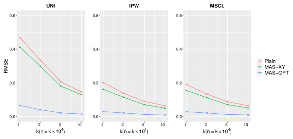
Figure 2: RMSE of different estimators under the Weibull model with $N=10^{6}$ and $n=k\times 10^{4}$.

Table 5: Bias and MSD of different estimators for the $j$-th dimension of $\text{\boldmath{$\theta$}}_{0}$ under the Weibull model with $N=10^{6}$. Plain: subsampling estimator without integrating sample moments; MAS-XY: moment-assisted subsampling estimator with $\bm{h}(\bm{x},y)=\bm{x}y$; MAS-OPT: moment-assisted subsampling estimator with $\bm{h}(\bm{x},y)=\check{\bm{h}}^{\rm opt}(\bm{x},y)$. The numbers in the Table are the results multiplied by 10.

$j$	UNI						IPW
	Plain		MAS-XY		MAS-OPT		Plain		MAS-XY		MAS-OPT
	Bias	MSD	Bias	MSD	Bias	MSD	Bias	MSD	Bias	MSD	Bias	MSD
$n=2000$
1	0.02	0.09	0.02	0.09	-0.02	0.01	0.01	0.09	-0.01	0.09	-0.01	0.01
2	0.01	0.24	0.02	0.23	-0.01	0.05	0.00	0.20	-0.02	0.19	0.00	0.06
3	0.02	0.38	0.06	0.21	-0.01	0.10	0.01	0.30	0.01	0.23	0.00	0.12
4	0.03	0.39	0.04	0.22	-0.01	0.10	0.01	0.30	0.01	0.23	0.00	0.11
5	-0.01	0.40	0.05	0.22	-0.01	0.10	0.01	0.28	0.02	0.22	0.00	0.11
6	-0.02	0.39	0.03	0.22	-0.01	0.10	-0.01	0.28	0.01	0.23	-0.01	0.12
7	0.02	0.40	0.05	0.22	-0.01	0.10	0.01	0.28	0.02	0.23	-0.01	0.12
8	0.01	0.39	0.04	0.22	-0.01	0.10	-0.02	0.28	0.00	0.22	-0.01	0.12
9	0.01	0.40	0.05	0.22	0.00	0.10	0.00	0.28	0.02	0.24	0.00	0.12
10	0.02	0.41	0.05	0.23	-0.01	0.09	0.01	0.29	0.01	0.23	0.00	0.12
11	0.00	0.40	0.05	0.21	-0.01	0.10	0.02	0.29	0.03	0.23	0.00	0.12
$n=10000$
1	0.00	0.04	0.00	0.04	0.00	0.00	0.00	0.04	0.00	0.04	0.00	0.01
2	0.00	0.11	0.00	0.10	0.00	0.02	0.00	0.08	0.00	0.08	0.00	0.03
3	0.01	0.17	0.01	0.09	0.00	0.04	0.00	0.13	0.00	0.10	0.00	0.06
4	0.00	0.17	0.01	0.09	0.00	0.04	0.00	0.13	0.00	0.11	0.00	0.05
5	-0.01	0.17	0.01	0.10	0.00	0.04	0.00	0.13	0.00	0.10	0.00	0.05
6	0.00	0.18	0.01	0.10	0.00	0.04	0.00	0.12	0.00	0.10	0.00	0.05
7	0.01	0.17	0.01	0.10	0.00	0.04	0.00	0.13	0.00	0.10	0.00	0.05
8	0.00	0.17	0.01	0.10	0.00	0.04	0.00	0.13	0.00	0.11	0.00	0.05
9	0.00	0.17	0.01	0.10	0.00	0.04	0.00	0.12	0.00	0.10	0.00	0.06
10	0.01	0.17	0.01	0.10	0.00	0.04	0.00	0.13	0.00	0.10	0.00	0.06
11	0.00	0.18	0.01	0.10	0.00	0.04	0.00	0.13	0.00	0.10	0.00	0.06

Table 6: CPU times (second) of different estimators under the logistic model with $N=10^{6}$ and $n=k\times 10^{4}$.

$k$	UNI			IPW
	Plain	MAS-XY	MAS-OPT	Plain	MAS-XY	MAS-OPT
0.1	0.30	0.82	1.64	2.51	2.86	3.74
0.2	0.54	1.02	1.82	2.74	3.09	3.89
0.5	1.06	1.51	2.17	3.11	3.38	4.16
1	1.90	2.31	2.93	3.90	4.16	4.88
Whole-data based estimator: 419.887

Similar observations are obtained from the simulation results here, demonstrating the effectiveness of MAS method in improving the estimation efficiency of subsampling methods under the Weibull model. Table 6 shows that the computing time of the six subsampling estimators is significantly shorter than that of the whole data based estimator. Compared with the logistic model, the whole data based estimator under the Weibull model takes longer to calculate, which further illustrates the necessity of the proposed method.

D.2 Numerical Evaluation of Variance Estimation

We compared the Monte Carlo standard deviation (MSD) and the estimated standard deviation (ESD) of the nine subsampling estimators listed in the main text to evaluate the performance of variance estimation. The results of $n=2000$ and $n=10000$ under the logistic and the Weibull models are presented in Tables 7 and 8, respectively.

Table 7: MSD and ESD of different estimators for the $j$-th dimension of $\text{\boldmath{$\theta$}}_{0}$ under the logistic model with $N=10^{6}$. Plain: subsampling estimator without integrating sample moments; MAS-XY: moment-assisted subsampling estimator with $\bm{h}(\bm{x},y)=\bm{x}y$; MAS-OPT: moment-assisted subsampling estimator with $\bm{h}(\bm{x},y)=\check{\bm{h}}^{\rm opt}(\bm{x},y)$. The numbers in the Table are the results multiplied by 10.

$j$	UNI						IPW						MSCL
	Plain		MAS-XY		MAS-OPT		Plain		MAS-XY		MAS-OPT		Plain		MAS-XY		MAS-OPT
	MSD	ESD	MSD	ESD	MSD	ESD	MSD	ESD	MSD	ESD	MSD	ESD	MSD	ESD	MSD	ESD	MSD	ESD
$n=2000$
1	0.46	0.46	0.46	0.46	0.10	0.10	0.43	0.45	0.43	0.44	0.10	0.10	0.43	0.45	0.42	0.44	0.10	0.10
2	0.77	0.79	0.56	0.57	0.19	0.18	0.77	0.76	0.56	0.54	0.19	0.18	0.76	0.76	0.55	0.54	0.19	0.18
3	0.79	0.79	0.56	0.57	0.19	0.18	0.75	0.76	0.53	0.54	0.18	0.18	0.74	0.76	0.52	0.54	0.18	0.18
4	0.79	0.79	0.57	0.57	0.19	0.18	0.76	0.76	0.55	0.54	0.19	0.18	0.75	0.76	0.54	0.54	0.19	0.18
5	0.75	0.79	0.57	0.57	0.18	0.18	0.74	0.76	0.54	0.54	0.18	0.18	0.73	0.76	0.54	0.54	0.18	0.18
6	0.80	0.79	0.58	0.57	0.19	0.18	0.74	0.76	0.54	0.54	0.18	0.18	0.73	0.76	0.53	0.54	0.18	0.18
7	0.79	0.79	0.57	0.57	0.18	0.18	0.74	0.76	0.54	0.54	0.19	0.18	0.73	0.76	0.54	0.54	0.19	0.18
8	0.82	0.79	0.58	0.57	0.19	0.18	0.76	0.76	0.58	0.54	0.18	0.18	0.74	0.76	0.57	0.54	0.18	0.18
9	0.79	0.79	0.58	0.57	0.18	0.18	0.75	0.76	0.56	0.54	0.19	0.18	0.74	0.76	0.55	0.54	0.19	0.18
10	0.79	0.79	0.58	0.57	0.19	0.18	0.76	0.76	0.55	0.54	0.19	0.18	0.76	0.76	0.55	0.54	0.19	0.18
$n=10000$
1	0.20	0.20	0.20	0.20	0.05	0.05	0.19	0.20	0.19	0.20	0.05	0.05	0.19	0.20	0.18	0.20	0.05	0.05
2	0.34	0.35	0.24	0.25	0.08	0.08	0.34	0.34	0.24	0.24	0.09	0.09	0.33	0.34	0.24	0.24	0.09	0.09
3	0.35	0.35	0.25	0.25	0.09	0.08	0.36	0.34	0.25	0.24	0.08	0.09	0.35	0.34	0.25	0.24	0.08	0.09
4	0.35	0.35	0.26	0.25	0.09	0.08	0.35	0.34	0.24	0.24	0.09	0.09	0.34	0.34	0.24	0.24	0.09	0.09
5	0.36	0.35	0.26	0.25	0.08	0.08	0.33	0.34	0.24	0.24	0.09	0.09	0.32	0.34	0.24	0.24	0.09	0.09
6	0.35	0.35	0.25	0.25	0.09	0.08	0.33	0.34	0.25	0.24	0.09	0.09	0.33	0.34	0.25	0.24	0.09	0.09
7	0.35	0.35	0.25	0.25	0.08	0.08	0.32	0.34	0.24	0.24	0.08	0.09	0.32	0.34	0.24	0.24	0.08	0.09
8	0.36	0.35	0.25	0.25	0.09	0.08	0.34	0.34	0.25	0.24	0.09	0.09	0.34	0.34	0.25	0.24	0.09	0.09
9	0.36	0.35	0.26	0.25	0.09	0.08	0.34	0.34	0.25	0.24	0.09	0.09	0.33	0.34	0.24	0.24	0.09	0.09
10	0.36	0.35	0.25	0.25	0.09	0.08	0.34	0.34	0.25	0.24	0.09	0.09	0.33	0.34	0.25	0.24	0.09	0.09

Table 8: MSD and ESD of different estimators for the $j$-th dimension of $\text{\boldmath{$\theta$}}_{0}$ under the Weibull model with $N=10^{6}$. Plain: subsampling estimator without integrating sample moments; MAS-XY: moment-assisted subsampling estimator with $\bm{h}(\bm{x},y)=\bm{x}y$; MAS-OPT: moment-assisted subsampling estimator with $\bm{h}(\bm{x},y)=\check{\bm{h}}^{\rm opt}(\bm{x},y)$. The numbers in the Table are the results multiplied by 10.

$j$	UNI						IPW
	Plain		MAS-XY		MAS-OPT		Plain		MAS-XY		MAS-OPT
	MSD	ESD	MSD	ESD	MSD	ESD	MSD	ESD	MSD	ESD	MSD	ESD
$n=2000$
1	0.09	0.09	0.09	0.08	0.01	0.01	0.09	0.09	0.09	0.09	0.01	0.01
2	0.24	0.24	0.23	0.22	0.05	0.05	0.20	0.20	0.19	0.19	0.06	0.06
3	0.38	0.39	0.21	0.21	0.10	0.09	0.30	0.29	0.23	0.22	0.12	0.11
4	0.39	0.39	0.22	0.21	0.10	0.09	0.30	0.29	0.23	0.22	0.11	0.11
5	0.40	0.39	0.22	0.21	0.10	0.09	0.28	0.29	0.22	0.22	0.11	0.11
6	0.39	0.39	0.22	0.21	0.10	0.09	0.28	0.29	0.23	0.22	0.12	0.11
7	0.40	0.39	0.22	0.21	0.10	0.09	0.28	0.29	0.23	0.22	0.12	0.11
8	0.39	0.39	0.22	0.21	0.10	0.09	0.28	0.29	0.22	0.22	0.12	0.11
9	0.40	0.39	0.22	0.21	0.10	0.09	0.28	0.29	0.24	0.22	0.12	0.11
10	0.41	0.39	0.23	0.21	0.09	0.09	0.29	0.29	0.23	0.22	0.12	0.11
11	0.40	0.39	0.21	0.21	0.10	0.09	0.29	0.29	0.23	0.22	0.12	0.11
$n=10000$
1	0.04	0.04	0.04	0.04	0.00	0.00	0.04	0.04	0.04	0.04	0.01	0.00
2	0.11	0.11	0.10	0.10	0.02	0.02	0.08	0.09	0.08	0.08	0.03	0.03
3	0.17	0.17	0.09	0.10	0.04	0.04	0.13	0.13	0.10	0.10	0.06	0.05
4	0.17	0.17	0.09	0.10	0.04	0.04	0.13	0.13	0.11	0.10	0.05	0.05
5	0.17	0.17	0.10	0.10	0.04	0.04	0.13	0.13	0.10	0.10	0.05	0.05
6	0.18	0.17	0.10	0.10	0.04	0.04	0.12	0.13	0.10	0.10	0.05	0.05
7	0.17	0.17	0.10	0.10	0.04	0.04	0.13	0.13	0.10	0.10	0.05	0.05
8	0.17	0.17	0.10	0.10	0.04	0.04	0.13	0.13	0.11	0.10	0.05	0.05
9	0.17	0.17	0.10	0.10	0.04	0.04	0.12	0.13	0.10	0.10	0.06	0.05
10	0.17	0.17	0.10	0.10	0.04	0.04	0.13	0.13	0.10	0.10	0.06	0.05
11	0.18	0.17	0.10	0.10	0.04	0.04	0.13	0.13	0.10	0.10	0.06	0.05

Tables 7 and 8 show that the estimated standard deviations are close to the Monte Carlo standard deviations for the proposed MAS estimator under both the logistic and the Weibull models and become closer as $n$ increases, which suggests that the proposed variance estimation is a reasonable estimator for the asymptotic variance.

D.3 Additional Application Results

In this section, we further explore the application of the proposed approach to airline data on a Windows server with a 24-core processor and 128GB RAM. The whole data-based estimator can be calculated on the server. We calculate the whole data-based estimator and treat it as the true parameter to calculate the bias of different subsampling estimators since the true parameter is unknown. The whole data-based estimate is $(-2.72,0.12,0.24,4.40,-0.01,-0.46,0.03)$. The computing time of the whole data-based estimator is $7662.96$ seconds. We repeat the subsampling process 200 times. The averaged CPU times of the nine subsampling estimators are presented in Table 9. From Table 9, it can be seen that even if the whole data-based estimator can be implemented with the available computational resources, the subsample estimators still have significant computational advantages over the whole data-based estimator. Moreover, we present the biases and MSDs of the nine subsampling estimators based on 200 replications in Table 10.

From Table 10, it can be seen that the biases of all the nine subsampling estimators are small. The Monte Carlo SDs of moment-assisted subsampling estimators are close to the corresponding estimated SDs in Table 3 of the main text. The SDs of the estimators moment-assisted estimators, especially with $\check{\bm{h}}^{\rm opt}(\bm{x},y)$, are much smaller than those of the corresponding plain estimators. These phenomena agree with the theoretical results in Theorem 1.

Table 9: The averaged CPU times (second) of different estimators in the airline data with $N=116,212,331$ and $n=50000$.

UNI			IPW			MSCL
Plain	MAS-XY	MAS-OPT	Plain	MAS-XY	MAS-OPT	Plain	MAS-XY	MAS-OPT
11.21	25.61	34.24	52.88	57.05	67.71	52.84	57.13	69.19

Table 10: Bias and MSD of different estimators for the $j$-th dimension of $\text{\boldmath{$\theta$}}_{0}$ in the airline data with $N=116,212,331$ and $n=50000$. The numbers in the Table are the results multiplied by 10.

$j$	UNI						IPW						MSCL
	Plain		MAS-XY		MAS-OPT		Plain		MAS-XY		MAS-OPT		Plain		MAS-XY		MAS-OPT
	Bias	MSD	Bias	MSD	Bias	MSD	Bias	MSD	Bias	MSD	Bias	MSD	Bias	MSD	Bias	MSD	Bias	MSD
1	-0.02	0.69	-0.02	0.69	0.02	0.06	-0.01	0.22	-0.01	0.21	0.00	0.04	0.02	0.22	0.02	0.22	0.00	0.04
2	-0.05	0.78	0.00	0.66	-0.02	0.07	0.02	0.29	0.03	0.23	0.00	0.05	0.01	0.28	0.02	0.24	-0.01	0.04
3	-0.01	0.73	0.00	0.64	-0.02	0.06	0.00	0.31	0.02	0.24	0.00	0.05	-0.01	0.32	0.00	0.26	0.00	0.05
4	0.07	0.82	0.05	0.78	-0.03	0.11	0.01	0.35	-0.01	0.30	0.00	0.05	-0.08	0.32	-0.07	0.26	0.00	0.05
5	0.09	0.78	0.03	0.66	0.01	0.08	-0.02	0.41	-0.04	0.30	0.00	0.05	-0.06	0.40	-0.05	0.30	0.00	0.05
6	0.04	0.79	0.02	0.64	0.01	0.08	-0.04	0.39	-0.02	0.28	0.00	0.05	0.04	0.37	0.03	0.27	0.00	0.05
7	-0.11	0.81	-0.08	0.68	0.01	0.09	0.02	0.37	0.02	0.28	0.00	0.05	0.08	0.37	0.06	0.26	0.00	0.05

References

• Ai et al. (2021a) Ai, M., Yu, J., Zhang, H., and Wang, H. (2021a), “Optimal Subsampling Algorithms for Big Data Regressions,” Statistica Sinica, 31, 749–772.
• Ai et al. (2021b) — (2021b), “Optimal subsampling for large-scale quantile regression,” Journal of Complexity, 62, 101512.
• Drineas et al. (2006) Drineas, P., Mahoney, M. W., and Muthukrishnan, S. (2006), “Sampling algorithms for $l_{2}$ regression and applications,” Proceedings of the seventeenth annual ACM-SIAM symposium on Discrete algorithm, 1127–1136.
• Fan et al. (2022) Fan, Y., Liu, Y., Liu, Y., and Qin, J. (2022), “Nearly optimal capture-recapture sampling and empirical likelihood weighting estimation for M-estimation with big data,” arXiv.
• Fithian and Hastie (2014) Fithian, W. and Hastie, T. (2014), “Local case-control sampling: Efficient subsampling in imbalanced data sets,” The Annals of Statistics, 42, 1693 – 1724.
• Han et al. (2020) Han, L., Tan, K. M., Yang, T., and Zhang, T. (2020), “Local uncertainty sampling for large-scale multiclass logistic regression,” The Annals of Statistics, 48, 1770 – 1788.
• Hansen (1982) Hansen, L. P. (1982), “Large Sample Properties of Generalized Method of Moments Estimators,” Econometrica, 50, 1029–1054.
• Hoffman and Wielandt (1953) Hoffman, A. J. and Wielandt, H. W. (1953), “The variation of the spectrum of a normal matrix,” Duke Mathematical Journal, 20, 37 – 39.
• Kushilevitz and Nisan (1996) Kushilevitz, E. and Nisan, N. (1996), Communication Complexity, Cambridge University Press.
• Newey (1994) Newey, W. K. (1994), “The asymptotic variance of semiparametric estimators,” Econometrica: Journal of the Econometric Society, 1349–1382.
• Team (2016) Team, R. C. (2016), “A Language and Environment for Statistical Computing,” R Foundation for Statistical Computing, Vienna, Austria. URL https://www.R-project.org.
• van der Vaart (2000) van der Vaart, A. W. (2000), Asymptotic Statistics, Cambridge University Press, New York.
• Wang (2019) Wang, H. (2019), “More Efficient Estimation for Logistic Regression with Optimal Subsamples,” Journal of Machine Learning Research, 20, 1–59.
• Wang and Kim (2022) Wang, H. and Kim, J. K. (2022), “Maximum sampled conditional likelihood for informative subsampling,” Journal of Machine Learning Research, 23, 1–50.
• Wang and Ma (2021) Wang, H. and Ma, Y. (2021), “Optimal subsampling for quantile regression in big data,” Biometrika, 108, 1–14.
• Wang et al. (2019) Wang, H., Yang, M., and Stufken, J. (2019), “Information-Based Optimal Subdata Selection for Big Data Linear Regression,” Journal of the American Statistical Association, 114, 393–405.
• Wang et al. (2018) Wang, H., Zhu, R., and Ma, P. (2018), “Optimal Subsampling for Large Sample Logistic Regression,” Journal of the American Statistical Association, 113, 829–844.
• Wu (1980) Wu, C.-F. (1980), “On Some Ordering Properties of the Generalized Inverses of Nonnegative Definite Matrices,” Linear Algebra and its Applications, 32, 49 – 60.
• Yao and Wang (2019) Yao, Y. and Wang, H. (2019), “Optimal subsampling for softmax regression,” Statistical Papers, 60, 585–599.
• Yu et al. (2022) Yu, J., Wang, H., Ai, M., and Zhang, H. (2022), “Optimal Distributed Subsampling for Maximum Quasi-Likelihood Estimators With Massive Data,” Journal of the American Statistical Association, 117, 1–12.