Learning Inertial Parameter Identification of Unknown Object with Humanoid Robot using Sim-to-Real Adaptation

Abstract

Understanding the dynamics of unknown object is crucial for collaborative robots including humanoids to more safely and accurately interact with humans. Most relevant literature leverage a force/torque sensor, prior knowledge of object, vision system, and a long-horizon trajectory which are often impractical. Moreover, these methods often entail solving non-linear optimization problem, sometimes yielding physically inconsistent results. In this work, we propose a fast learning-based inertial parameter estimation as more practical manner. We acquire a reliable dataset in a high-fidelity simulation and train a time-series data-driven regression model (e.g., LSTM) to estimate the inertial parameter of unknown objects. We also introduce a novel sim-to-real adaptation method combining Robot System Identification and Gaussian Processes to directly transfer the trained model to real-world application. We demonstrate our method with a 4-DOF single manipulator of physical wheeled humanoid robot, SATYRR. Results show that our method can identify the inertial parameters of various unknown objects faster and more accurately than conventional methods.

I INTRODUCTION

Humanoid robots have become increasingly prevalent with great potential in various fields where they are expected to interact and collaborate with humans in dynamics and unstructured environments such as manufacturing, healthcare, and even disaster response [1, 2]. To facilitate seamless and safe human-robot collaboration, humanoid robots need to possess an accurate understanding of the physical properties of objects they interact with. Leveraging the physical properties of an object, commonly referred to as the inertial parameter, including mass, center of mass (COM), and moment of inertia, can enable robots to robustly and adaptively interact in the real world. For instance, an accurate understanding of an object’s physical property could aid robots in carrying an object or throwing it into a precise location more accurately and safely, while insufficient information may lead robots to apply excessive or insufficient forces during manipulation tasks, resulting in unintended slipping and damage to the object.

Identifying the physical parameters of an unknown object with a humanoid robot is nontrivial and sometimes practically limited in certain situations due to several inherent challenges: (1) the presence of noisy signals from force-torque sensors, (2) reliance on assumed knowledge of object geometry using CAD files, (3) the necessity of visual or perception sensors to discern object pose and shape, and (4) the requirement for long excitation trajectories to collect sufficient data. Considering the interaction with a wide variety of objects in an uncontrolled situation, prior knowledge of objects is not always accessible, and a fast identification method is necessary for the stability and task efficiency of a robot.

In this paper, a fast learning-based approach to identify the full set of inertial parameters of an unknown object is proposed. The key ideas are two holds: (1) discerning an object’s dynamic properties in a non-direct manner by employing the history of the robot’s proprioceptive states influenced by the different object dynamics (2) utilizing a simulation to accurately calculate the true inertial parameters of unidentified objects. A data-driven regression model is trained in the simulation and is transferred to the real world via the proposed sim-to-real adaptation method. To the best of our knowledge, this is the first work in which a fast inertial parameter estimation for unknown objects is achieved through the sim-to-real adaptation method, thereby bringing our main contribution. Unlike previous works, our method doesn’t need to use a prior knowledge of an object, and even a camera system. We also propose a novel sim-to-real adaptation method combining Robot System Identification (SysID) and Gaussian Processes (GPs).

Figure 1: Conceptual overview of the proposed method. Thousands of wheeled humanoid robots, SATYRR, in IssacGym Simulator. Consecutive shaking motion ((A) to (D)) to estimate the inertial parameter of an unknown object with SATYRR. A physical SATYRR robot with shaking an object.

II RELATED WORK

Research on inertial parameter identification of rigid bodies has a rich history [3]. Given that the dynamics model of a multi-body system (e.g., humanoid robot or manipulator) is linear with respect to the inertial parameter, a linear least squares method has been widely used as a popular choice for identifying this parameter, whether through offline or adaptive means. However, this traditional approach has several limitation that has to be further considered.

Without including constraints in the optimization process, not all combinations of parameters correspond to the physical system. Some literature has explored incorporating physical consistency as part of constraints to obtain more realistic inertial parameters [4, 5, 6, 7]. They propose the custom manifold optimization [4], the use of linear matrix inequalities (LMI) in convex constraints [5], and Reimmannian metrics [7], respectively, and enable physical consistency of the identified parameters. However, their method takes more than 6 seconds and requires prior knowledge of an object (e.g., the shape of each rigid body, bounding box estimated from CAD) which is not always accessible. In this work, dynamic consistency of inertial parameters is implicitly enforced using regularization. Moreover, the parameter estimation including a trajectory generation takes within 0.6 seconds.

Force-torque sensors (FT) are commonly leveraged to determine the inertial parameter of an object [8, 9, 10]. They are required to be positioned at the joints or wrist of a manipulator. However, commercial FT sensors are heavy and expensive, and are very noisy with an unknown drifting bias [11]. A force/torque estimation is another relevant approach [12, 13]. They employ the neural network to estimate joint torque, though this still necessitates the use of motor torque sensors. In [14], author propose learning-based inertial parameter estimator using encoder discrepancies and attention mechanism, while they identify only the mass and COM of an object. Unlike these approaches, our method can directly estimate the full set of inertial parameters of unknown object without using a torque/force sensor and the estimation technique.

With the rapid growth of deep learning techniques, learning-based inertial parameter estimation has been actively studied [15, 16, 17, 18]. Most of them utilized extensive visual datasets comprised of elements like images and video sequences. While accessing a visual dataset is not challenging, interacting with the object remains an inevitable process in estimating its dynamics, due to the limited information such as density. Our approach only relies on interacting with an object and doesn’t require to use camera. Moreover, to get a large amount of dataset efficiently, we used a simulation environment and proposed domain adaptation method to reduce the reality gap.

In recent years, research on sim-to-real adaptation has garnered considerable attention. Under a high-level idea of Domain randomization [19], privileged learning [20, 21], system identification [22], bayesian optimization [23, 24], and deep neural network [25]. While these approaches have shown promising result in robotics, a perfect match between two trajectories obtained from two domain are still very challenging.

III BACKGROUND

The inertial parameters of $i$’th rigid-body are collected as $\mathbf{\bm{\phi}}_{i}=[m_{i},\mathbf{c}_{i}^{\top},I^{xx}_{i},I^{yy}_{i},I^{zz}_{i},I^{xy}_{i},I^{yz}_{i},I^{zx}_{i}]^{\top}\in\mathbb{R}^{10}$, where $m\in\mathbb{R}$ is the mass, $\mathbf{c}=[c_{x},c_{y},c_{z}]^{\top}\in\mathbb{R}^{3}$ is the the center of mass (COM) position, and $I^{(\cdot)}$ are the moments and the products of inertia. In the classical way, the inertial parameters of $n_{s}$-rigid-body system can be estimated by classical linear regression model $\mathbf{\bm{Y}}(\mathbf{\bm{a}},\mathbf{\bm{\omega}},\dot{\mathbf{\bm{\omega}}})$ using the rigid body dynamics,

$$\begin{bmatrix}\mathbf{\bm{f}}\\ \mathbf{\bm{\tau}}\end{bmatrix}=\begin{bmatrix}m\mathbf{\bm{a}}\\ [\mathbf{\bm{\omega}}]\mathbf{\bm{I}}\mathbf{\bm{\omega}}+\mathbf{\bm{I}}\dot{\mathbf{\bm{\omega}}}\end{bmatrix}=\mathbf{\bm{Y}}\phi.$$ (1)

where the symbolic $\mathbf{\bm{f}}\in\mathbb{R}^{3}$ and $\mathbf{\bm{\tau}}\in\mathbb{R}^{3}$ denote forces and torques, respectively. The term $m\in\mathbb{R}^{+}$ denotes the mass, $\mathbf{\bm{a}}\in\mathbb{R}^{3}$ is the linear acceleration, $\mathbf{\bm{\omega}}\in\mathbb{R}^{3}$ is the angular velocity, $\dot{\mathbf{\bm{\omega}}}\in\mathbb{R}^{3}$ is the angular acceleration, and the bracket denotes $[\,\cdot\,]$ the skew-symmetric representation of a vector.

A simplistic estimation of inertial parameters with least-square regression may result in physically invalid parameters [5]. Hence, the regression could be enforced with positive-semi definiteness of mass and inertia tensor as follows, —s— ϕ∑_j=1^n_s ∥ Y_j ϕ_j - τ_j ∥ ^2 m≥0, σ_k≥0, k=1,2,3 σ_1 + σ_2 + σ_3≥2σ_k, k=1,2,3 to enforce the positive-semidefinitene of mass and inertia tensor $\eqref{opti:mass}$ and a triangular inequality$\eqref{opti:tri}$, where $\sigma_{(\cdot)}$ denotes the eigenvalues of the inertia tensor of a rigid body. In our case, we implicitly consider dynamic consistency by using the regularization (see Eq. 11).

IV METHODOLOGY

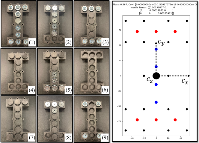
Figure 2: Left Side: Design of different objects. Depending on the location of the weights, the object can be represented as a barbell(3), hammer(8), etc. Right Side: Visual sample of an object(3) with ground truth inertial parameters. The CoM is defined based on a central fixed coordinate system.

Our framework consists of two distinct steps: 1) Sim-to-Real Adaptation aimed at enhancing the fidelity of the simulation via Robot System Identification (SysID) for a SATYRR robot and Gaussian Processes (GPs); and 2) Learning the full set of inertial parameters for an unknown object via time-series data-driven regression model. Our estimator trained in the simulator can be directly applied to a physical SATYRR robot without requiring further manual tuning. The overview of the proposed method is described in Algorithm 1.

IV-A Target System Description and Unknown Object Design

In this work, we utilize a four degrees-of-freedom (DoF) manipulator of a wheeled humanoid, SATYRR [26], to hold and shake an object. As a preliminary step, to simplify the problem by minimizing the effect of the dynamics of whole-body SATYRR, we fix its torso and lower body. Inspired by the previous work [27], our object is designed to easily and precisely calculate the ground truth inertial parameter of various objects. This object consists of a combination of three cuboids, ten-cylinder holes, and steel weights. These weights can be placed in ten different locations as depicted in Fig.2. The ground truth of inertial parameters can be calculated based on the moment of inertia, the density of each weight, and the size of each cuboid.

IV-B High-Fidelity Simulator and Sim-to-Real Adaptation

Samples drawn from the source (simulation) and target (real-world) distribution, $\mathcal{D}^{s}\sim p_{s}(\bm{X}_{S},\mathbf{\bm{y}}_{S})$ and $\mathcal{D}^{t}\sim p_{t}(\bm{X}_{T},\mathbf{\bm{y}}_{T})$ typically differ ($\mathcal{D}^{s}\in\mathcal{D}_{S}$ and $\mathcal{D}^{t}\in\mathcal{D}_{T}$). In terms of dynamics, reality gap (sim-to-real gap) $\delta$ is caused by the combination of inaccurate parameters of the parametric model, non-parametric uncertainties, etc. The reality gap regarding nonlinear dynamics of a multi-body system can be represented as follows:

$$\delta_{t}=f_{t}^{\text{real}}(\mathbf{\bm{x_{t}}},\mathbf{\bm{u_{t}}})-\hat{f}_{t}^{\text{sim}}(\mathbf{\bm{\hat{x}_{t}}},\mathbf{\bm{\hat{u}_{t}}})+w_{t}^{\text{real}}-w_{t}^{\text{sim}}$$ (2)

Here, $f_{t}^{\text{real}}$ and $\hat{f}_{t}^{\text{sim}}$ represent the nonlinear functions dictating real-world and simulated dynamics at time $t$, respectively ($x_{t+1}=f(x_{t},u_{t})$). The variables $w_{\text{real}}$ and $w_{\text{sim}}$ denote process noise, while $\mathbf{\bm{x}}$ and $\mathbf{\bm{\hat{x}}}$ indicate states, and $\mathbf{\bm{u}}$ and $\mathbf{\bm{\hat{u}}}$ are the control efforts in the real and simulated environments, respectively. The error $\delta$ can be further decomposed into a parametric model $\delta\hat{f}$ and non-parametric model $\delta\hat{g}$ as follows:

$$\delta_{t}=\delta\hat{f}(\mathbf{\bm{\hat{x}_{t}}},\mathbf{\bm{\hat{u}_{t}}}|\bm{\zeta})+\delta\hat{g}(\mathbf{\bm{\hat{x}_{t}}},\mathbf{\bm{\hat{u}_{t}}})$$ (3)

where the system parameters $\bm{\zeta}$, the estimated states $\mathbf{\bm{\hat{x}}}$ , the control effort $\mathbf{\bm{\hat{u}}}$, and time $t$. To compensate for the error caused by $\delta\hat{f}$ and $\delta\hat{g}$, we leverage the SysID and GPs. Note that both methods are employed to account for the dynamics discrepancy in the robot itself, arising due to the reality gap. Ensuring that this adjusted model is generalizable is essential, especially when the robot handles unfamiliar objects. This concept is closer to domain adaptation than that of domain randomization [21, 28] because the goal is to match two different trajectories obtained from disparate domains rather than building a robust controller.

Algorithm 1 Procedure of Learning Inertial Parameter Estimation of unknown Object via Sim-to-Real Adaptation

Phase 1 Robot System Identification

Input: $\mathcal{D_{T}}=\{D^{1}_{T},D^{2}_{T},\dots,D^{m}_{T}\},m=5$

Initialize: $\zeta\in\mathbb{R}^{k}$, $\mathcal{L}\in\mathbb{R},k=8$

while until $(\mathcal{L}\text{ converges})$ do

     $({\bm{X}^{i}_{T},\mathbf{\bm{y}}^{i}_{T})}^{m}_{i=1}\leftarrow\mathcal{D_{T}}$

     $({\bm{X}^{i}_{S},\mathbf{\bm{y}}^{i}_{S})}\leftarrow\hat{f}(\cdot|\zeta)_{sim}$ $\triangleright$ Run IssacGym Simulator

     Calculate the Loss function $\mathcal{L}$ $\triangleright$ Eq. (4)

     Update parameter $\zeta$ via particle swarm optimization

     Return: $\zeta^{*}$

end while

Phase 2 Gaussian Processes

Input: Gaussian Processes $\mathcal{GP}$, Simulation with SysID applied $\hat{f}(\cdot|\zeta^{*})_{sim}$, and $\mathcal{D_{T}}$

do

    $({\bm{X}^{i}_{T},\mathbf{\bm{y}}^{i}_{T})}^{m}_{i=1}\leftarrow\mathcal{D_{T}}$

    $({\bm{X}^{i}_{S},\mathbf{\bm{y}}^{i}_{S})}\leftarrow\hat{f}(\cdot|\zeta^{*})_{sim}$

    Calculate non-parametric modeling error $\hat{g}(\mathbf{\bm{\hat{x}}},\mathbf{\bm{\hat{u}}},t)$

    Optimize a GP regression model using GPy. $\triangleright$ Eq. (5)

    Save a GP model $\mathcal{GP}(\mu,k)$

    Apply the $\mathcal{GP}(\mu,k)$ to the simulation $\hat{f}(\cdot|\zeta^{*})_{sim}$

    Return: $\hat{f}(\cdot|\zeta^{*},\mathcal{GP})_{sim}$

end

Phase 3 Learning Inertial Parameter of an Object

Input: $\mathcal{D_{S}}\leftarrow\hat{f}(\cdot|\zeta^{*},\mathcal{GP})_{sim},\mathcal{L_{NN}}$

while until $(\mathcal{L_{NN}}\text{ converges})$ do

         Training a time-series data-driven model IV-C3

         to minimize the loss $\mathcal{L_{NN}}$ $\triangleright$ Eq. (11)

end while

IV-B1 Offline Robot System Identification

The goal of SysID is to minimize the discrepancy between $\bm{X}^{t}_{S}$ and $\bm{X}^{t}_{T}$ by searching for more realistic system parameter $\bm{\zeta}$. The cost function can be some distance function $d(\cdot|\cdot)$ over a dataset of $m$ samples where $T$ is the length of each sample (Eq. (4)). We chose the mean square error (MSE) as a $d$ function to match the different trajectories.

$$\mathcal{L}=\operatorname*{arg\,min}_{\bm{\zeta}}\dfrac{1}{m}\sum_{i=1}^{m}\sum_{t=1}^{T}d(\bm{X}^{t}_{S},\bm{X}^{t}_{T}).$$ (4)

The optimal parameter $\bm{\zeta}^{*}$ can be chosen by solving the Eq. 4 and we utilized the PSO algorithm due to its global search ability and fast convergence speed. In this work, the parameters $\zeta\in\mathbb{R}^{8}$ to be optimized contain joint damping $d_{j}\in\mathbb{R}^{4}$ and link mass $m_{l}\in\mathbb{R}^{4}$. To make a more realistic simulation environment, we chose the PD controller gain ($K_{p}\in\mathbb{R}^{4},K_{d}\in\mathbb{R}^{4}$) considering the real-world gain applied to SATYRR.

IV-B2 Non-Parametric Dynamics Modeling via Gaussian Processes

To model non-parametric dynamics, we leverage the GPs considering its benefit of sample efficiency and potential to construct a wide range of functions without assuming a specific functional form [29]. The non-parametric dynamics model $\hat{g}$ can be formulated with GPs as follows:

$$\hat{g}(\mathbf{\bm{\hat{x}_{t}}},\mathbf{\bm{\hat{u}_{t}}})=\mathcal{GP}(\mu(\mathbf{\bm{\hat{x}_{t}}},\mathbf{\bm{\hat{u}_{t}}}),k(\mathbf{\bm{\hat{x}_{t}}},\mathbf{\bm{\hat{u}_{t}}},\mathbf{\bm{\hat{x}_{t^{\prime}}}}^{\prime},\mathbf{\bm{\hat{u}_{t^{\prime}}}}^{\prime})).$$ (5)

here, the individual terms represent the state $\mathbf{\bm{\hat{x}}}$, control effort $\mathbf{\bm{\hat{u}}}$, and time $t$. The GPs $\mathcal{GP}(\mu,k)$ is expressed with a mean function $\mu$ and covariance function $k$ where the mean $\mu(\mathbf{\bm{\hat{x}_{t}}},\mathbf{\bm{\hat{u}_{t}}})$ represents the expected value of the process at each point in the input space and the covariance function $k(\mathbf{\bm{\hat{x}_{t}}},\mathbf{\bm{\hat{u}_{t}}},\mathbf{\bm{\hat{x}_{t^{\prime}}}}^{\prime},\mathbf{\bm{\hat{u}_{t^{\prime}}}}^{\prime})$ describes the correlation between outputs for two distinct sets of inputs in the function $\hat{g}$. We constructed and optimized the GP regression model using the GPy library. Radial Basis Function (RBF) kernel (both variance and length scale set to 1) is utilized.

IV-C Learning Inertial Parameter of unknown object

IV-C1 Dynamic Trajectory Planning and Manipulation Control

periodic excitation trajectories are widely used to generate data for dynamic model identification [5, 27, 30]. These are typically based on the Fourier series and a combination of trigonometric functions [31]. Although they showed quite sufficient performance to identify a full set of inertial parameters, the total operation time is quite long (e.g., 35 seconds in [27]). Inspired by how humans identify and guess an unknown object by shaking it (e.g., amplitude and frequency of behavior decreases over time), we designed the dynamic trajectory as follows.

$$f(t)=h_{\text{freq}}-(h_{\text{freq}}-l_{\text{freq}})t\hskip 14.22636pt\phi(T)=\Delta t\sum_{\tau=0}^{T}f(\tau)$$ (6)

$$w(t)=\frac{1}{2}\left(1-\cos\left(\frac{2\pi t}{T_{\text{total}}}\right)\right)$$ (7)

$$X(t)=\alpha\sin(2\pi\phi(T))w(t)$$ (8)

where the frequency is defined by $f(t)$, which starts at $h_{\text{freq}}$ and linearly decreases to $l_{\text{freq}}$. The phase of the signal, $\phi$ is then computed as the cumulative sum of the frequency, scaled by the time step. The sinusoidal trajectory is given by $X(t)$ where the amplitude is scaled by a factor $\alpha$ and further modulated by a Hann window, $w(t)$, to ensure smooth transitions at the start and end of the trajectory. The trajectory $X(t)$ is applied to the end-effector in $x$ and $y$ axis ($T_{total}=0.5$, x-axis: $h_{freq}=5,l_{freq}=1,\alpha=-5$, y-axis: $h_{freq}=3,l_{freq}=1,\alpha=80$).

The numerical inverse kinematics using a pseudo-inverse Jacobian of the 4-DoF manipulator is employed to control the manipulator of SATYYR, which is defined as

$$J^{+} =(J^{T}J+\lambda^{2}I)^{-1}J^{T},$$ (9)

$$\theta_{des} =\theta+\alpha J^{+}e.$$

where $J^{+}$ represents a pseudo-inverse Jacobian leveraging a Damped Least Squares method, aiding to improve stability near a singular configuration and dealing with noisy data or slight modeling errors by utilizing regularization. The symbol $\lambda$ is damping, $\alpha$ is a hyperparameter, and $e=x_{des}-x$ is task-space position error.

IV-C2 Database Construction

To build a learning-based object dynamics estimator, we constructed the $M$ number of source dataset $\mathcal{D}_{S}={(\bm{X}^{i}_{S},\bm{y}^{i}_{S})}^{M}_{i=1}(M=5000)$ in IssacGym simulator [32] (5,000 environments are utilized at the same time). To directly apply the pre-trained estimation model to the SATYRR without further manual tuning, we employed a more realistic simulator IV-B to acquire the dataset $\mathcal{D}_{S}$. All agents in the simulator track the desired trajectory (Eq. 8) while holding different objects. The estimator takes as input the concatenated vector $\bm{X}$ and outputs estimated inertial parameter $\bm{y}$ as:

$$\bm{X}=[q^{1}_{t:T},q^{2}_{t:T},q^{3}_{t:T},q^{4}_{t:T},\dot{q}^{1}_{t:T},\dot{q}^{2}_{t:T},\dot{q}^{3}_{t:T},\dot{q}^{4}_{t:T}]^{\top}$$ (10)

$$\bm{y}=[m,c_{x},c_{y},c_{z},I_{xx},I_{yy},I_{zz}]^{\top}$$

where $q^{i}_{t:T}$ and $\dot{q}^{i}_{t:T}$ are the history of joint position and velocity of each joint, respectively. The term $\bm{y}$ denotes the vector of inertial parameters. We simplify the problem by focusing on estimating the diagonal terms in the inertia matrix considering a more tractable analysis while retaining the essential physics of the problem. To collect the database in the world, a wheeled humanoid robot, SAYTRR [26] tracked the pre-recorded shaking motion created in simulation (see Eq. (10). A total of ten different objects were involved, along with a free case where no object was held. For each object case, the trajectory was applied to the SATYRR five times (i.e., a total of 50 real-world dataset were obtained for the validation in the experiment).

IV-C3 Training Time-Series Data-Driven Model with Constrained Dynamic Consistency

To learn the inertial parameter $\phi$, we developed a data-driven estimator by training a time-series data-driven regression model (e.g., LSTM) using 4000 samples of the training set in dataset $\mathcal{D}_{S}$ (500 for validation set and 500 for test set). Dynamic consistency is implicitly taken into account by applying the regularization term in the loss function to estimate more physically reliable parameters. The total loss function considering dynamic consistency is defined as

$$\mathcal{L_{NN}}=w_{1}\frac{1}{n}\sum_{i=1}^{n}(y_{i}-\hat{y}_{i})^{2}+w_{2}\mathcal{L_{\text{tri}}}+w_{3}\mathcal{L_{\text{pos}}}\hat{y}$$ (11)

$$\mathcal{L_{\text{tri}}}(I_{xx},I_{yy},I_{zz})=\sum_{\alpha\neq\beta\neq\gamma}^{1,2,3}\log\big{(}1+\exp(I_{\alpha}-I_{\beta}-I_{\gamma})\big{)}$$

$$\mathcal{L_{\text{pos}}}\hat{y}=\log(\lambda)\sum_{i=1}^{N}\left|\min\left(\text{output}_{i,k},0\right)\right|,\ k=[0,4,5,6]$$

where the total loss $\mathcal{L_{NN}}$ combines mean square error, triangular inequality loss $\mathcal{L_{\text{tri}}}(I_{xx},I_{yy},I_{zz})$, and negative output penalization loss $\mathcal{L_{\text{pos}}}\hat{y}$. The term $w_{1},w_{2}$, and $w_{3}$ are the weight of each term and are decided by manual tuning ($w_{1}=0.5,w_{2}=0.3,w_{3}=0.2$) considering the importance of each parameter. We trained and tested a LSTM for 2,000 epochs, using a batch size of 512 and a learning rate of 1e-3, with a weight decay of 1e-5. The hidden size of LSTM is 1024 and four layers are utilized.

V EXPERIMENT

The proposed learning-based inertial parameter identification method is verified with a 4-DOF manipulator of SATYRR [26] in both a simulation and the real world. The experimental setup is illustrated in Fig. 1 and Fig. 2. The purpose of experiments is to address the following questions: (1) How advantage our real-to-sim method help reduce a reality gap? (2) How fast and accurate is our framework compared to the previous works in estimating the inertial parameters of an unknown object? (3) Ablation Studies: How much does the inclusion of torque information enhance estimation accuracy? What data-driven regression model shows the best estimation performance?

V-A Experimental Plan

V-A1 Sim-to-Real Adaptation

We evaluate the sim-to-real adaptation ability by comparing five separate baselines: (a) PureSim: simulation using default physics parameters and PD controller with almost perfect tracking performance (b) Sim+ActuatorNet: using Actuator Network [21] instead of PD controller. We collected a dataset from SAYTRR and trained the Actuator Network defined as

$$\tau_{j}=jR(q^{*}_{j},q_{j},\dot{q}^{*}_{j},\dot{q}_{j},K_{p},K_{d}),\hskip 14.22636ptj=1,2,3,4$$ (12)

where desired joint position and velocity $q^{*}$ and $\dot{q}^{*}$, actual joint position and velocity $q$ and $\dot{q}$, and controller gain $K_{p}$ and $K_{d}$. (c) Sim+GPs: applying the GPs into PureSim (d) Sim+SysID: applying the SysID into PureSim (e) Sim+SysID+GPs (Ours): Applying the GPs to (d). To verify the performance of sim-to-real adaptation, the mean sqaure error (MSE, Eq. 4) is used as an evaluation index. Note that the GP model is trained only with training data that does not contain an object to demonstrate the generalizability against various unknown objects.

V-A2 Inertial Parameter Estimation

We compared the performance of our framework against the following baselines: (1) Ordinary Least Squares (OLS) [3] and (2) Weighted Least Squares (WLS) [30]. Since these traditional methods require to use of a force/torque sensor, we utilized 500 samples of the test dataset obtained from the simulation (Ours) to directly assess a force and a torque value. For a fair comparison, we used the open-source (MATLAB) provided by the authors [3, 30]. The mean absolute error (MAE=$|\hat{y}_{k}-y_{k}|$) and the normalized MAE (NMAE= $\frac{1}{n}\sum_{k=1}^{n}\frac{|\hat{y}_{k}-y_{k}|}{y_{\text{scale}}}$ ) are leveraged as evaluation indexes.

V-A3 Ablation Studies

We examine (1) how joint torque usage affects inertial parameter estimation performance, and (2) the performance of various deep learning models that are developed for a similar purpose (e.g., targeting the time-series data). All models are trained and tested with the same dataset (Sim+SysID+GPs (Ours)). The first ablation study is notable for exploring the trade-off between estimator accuracy and sim-to-real adaptation. This stems from the fact that while utilizing torque information typically enhances estimation accuracy, it can also increase the reality gap. Here, the Actuator Network is employed to estimate a realistic joint torque per actuator.

TABLE I: Results of Real to Sim Transfer. SysID and GPs are developed with only training data, which means that they have no knowledge of the dynamics of different objects in the evaluation process.

		PureSim	Sim +ActuatorNet	Sim+GP	Sim +SysID	Sim+SysID +GP(Ours)
	Training Data (Free)	0.5503	0.4145	0.0	0.0846	0.0
	Full Steel	0.9622	0.8636	0.28	0.3635	0.2638
	Full ABS	0.5644	0.4879	0.0026	0.0762	0.0031
	Full ABS Half	0.5975	0.5507	0.0056	0.091	0.0041
	Half and Half	0.4778	0.4624	0.102	0.0512	0.0223
	Barbell	0.6079	0.5025	0.0089	0.0813	0.0062
	Corner	0.7085	0.5971	0.0932	0.1808	0.091
	Hammer	0.5873	0.652	0.0063	0.0085	0.0052
	Tee	0.4882	0.598	0.0091	0.055	0.0199
	Empty	0.5993	0.5408	0.0053	0.0942	0.0041
MSE (rad)	Average	0.6143	0.5669	0.0513	0.10863	0.04197

TABLE II: Results of Inertial Parameter Estimation of Unknown Objects Both In a Simulation and the Real-World. In each column, results show mean and standard deviation (in parentheses), respectively. Inertia Matrix is expressed with I-Mat. Same applies to TableIII. Parameters are mass ($m$), CoM ($\mathbf{\bm{c}}$), and Inertia Matrix ($I^{(\cdot)}$). Units are kg, m, and $kgm^{2}$.

	Simulation										Real-World
	PureSim		Sim +ActuatorNet		Sim+GP		Sim +SysID		Sim+SysID +GP(Ours)		PureSim		Sim +ActuatorNet		Sim+GP		Sim +SysID		Sim+SysID +GP(Ours)
	MAE	NMAE	MAE	NMAE	MAE	NMAE	MAE	NMAE	MAE	NMAE	MAE	NMAE	MAE	NMAE	MAE	NMAE	MAE	NMAE	MAE	NMAE
$m$	0.031 (0.031)	0.054 (0.074)	0.013 (0.015)	0.033 (0.173)	0.021 (0.023)	0.035 (0.046)	0.026 (0.026)	0.044 (0.055)	0.038 (0.033)	0.076 (0.133)	0.49 (0.222)	1.323 (0.908)	0.26 (0.147)	0.522 (0.202)	0.798 (0.201)	2.134 (1.19)	0.437 (0.147)	1.215 (0.773)	0.084 (0.054)	0.208 (0.149)
$\mathbf{\bm{c}}$	0.009 (0.006)	8.415 (6.683)	0.009 (0.006)	9.255 (6.353)	0.009 (0.006)	8.256 (6.779)	0.009 (0.007)	9.117 (7.098)	0.01 (0.007)	9.923 (7.47)	0.009 (0.006)	7.429 (5.645)	0.004 (0.003)	2.791 (2.241)	0.011 (0.005)	9.438 (3.331)	0.004 (0.004)	2.958 (3.761)	0.007 (0.005)	7.36 (5.639)
$I^{(\cdot)}$	0.017 (0.005)	32.37 (72.02)	0.014 (0.002)	31.57 (83.53)	0.016 (0.003)	25.062 (31.53)	0.016 (0.007)	34.074 (76.3)	0.014 (0.002)	30.57 (62.89)	0.014 (0.009)	14.00 (13.99)	0.016 (0.001)	32.02 (11.15)	0.034 (0.006)	71.55 (22.33)	0.015 (0.0015)	23.93 (6.911)	0.016 (0.0023)	31.96 (13.65)

VI RESULTS AND DISCUSSION

VI-A Sim-to-Real Adaptation Experiments

The results of sim-to-real adaptation are summarized in Table I. Applying SysID to PureSim can substantially reduce the reality gap across all object cases, and further application of GPs on the SysID results can decrease the gap even more. This suggests that each method is efficient in narrowing the reality gap resulting from the error of the parametric model and non-parametric model, individually. The Sim+SysID+GP shows a better performance than the Sim+GP even though the Sim+GP can also perfectly represent the error in the training dataset. This is because the parametric model can be more generalizable than the GP model. This may give us insight and motivation that employing a more accurate dynamics model with its identified parameter has the potential to further reduce the reality gap. Interestingly, we also empirically observed that if the residual error is too small, the performance of GPs decreases. Our method underperforms in the full steel case, indicating potential degradation with larger objects.

We also examine how the sim-to-real adaptation affects the estimation performance (see Table II). We observed that the Sim+SysID+GP significantly improves the estimation performance regarding mass, whereas exhibiting a similar performance in other properties in the real world. This may be because only mass is not influenced by the measurement error of ground-truth value as well and the scale of other properties is very small, resulting in the high sensitivity of accuracy. However, this still suggests that the results of the estimator are consistent with the results of the sim-to-real adaptation. With the simulation dataset, all methods show similar estimation performance.

VI-B Inertial Parameter Estimation

We compare the inertial parameter estimation performance against conventional methods in terms of accuracy, speed, and dynamic consistency. The proposed learning-based estimator achieved the best performance in estimating the inertial parameter of unknown objects with SATYRR. (see Ours in Table II, and OLS and WLS in Table III). The WLS shows a slightly better estimation performance than the OLS. Since we utilize the trajectory data recorded for 0.5 seconds, the total estimation time is almost 0.5 seconds (inference time for a learning-based estimator is less than 0.01 seconds). To the best of our knowledge, as considering the overall time for the estimation ranging from trajectory generation to the optimization process in a classical approach, our method is the fastest inertial parameter estimation compared to other previous methods. In addition, all outcomes from 500 samples satisfy the physical consistency.

VI-C Ablation Studies

As shown in Table II and Table III, feeding additional joint torque information into a time-series data-driven model is beneficial in improving the estimation performance in a simulation. However, its performance in the real-world is much worse than the models without using the joint torque information. This is because additional information results in a larger reality gap. This raises the interesting research question: How can additional information be used efficiently without increasing the reality gap? As shown in Fig. 3, LSTM achieves the best performance among four different time-series data-driven models. We observed that our method is not very sensitive to using different types of data-driven regression models.

VI-D Limitations

Our research has several limitations to be further improved. Firstly, we approximate the inertia matrix as a diagonal matrix, assuming that the off-diagonal elements are negligible. To make our method more generalizable, We will consider the full elements of inertia tensor in future work. Secondly, our method is dependent on the defined trajectory. Real-time sim-to-real adaptation method and trajectory optimization are interesting future works. Thirdly, considering applying our method to humanoid robots (e.g., SATYRR), the incorporation of the full-body dynamics of the humanoid is necessary. Combining the robot dynamics and a neural network (e.g., a physics-informed neural network) can be a potential solution.

TABLE III: Results of Inertial Parameter Estimation and Ablation Studies.

	Experiment 2					Ablation Studies
	OLS (Sim)		WLS (Sim)			Ours (Sim) (W/Torque)		Ours (Real) (W/Torque)
	MAE	NMAE	MAE	NMAE		MAE	NMAE	MAE	NMAE
Mass (kg)	0.07 (0.058)	0.097 (0.048)	0.066 (0.058)	0.097 (0.062)		0.014 (0.014)	0.026 (0.037)	0.47 (0.28)	1.359 (1.055)
CoM (m)	0.094 (0.022)	88.35 (23.23)	0.082 (0.028)	77.09 (29.80)		0.009 (0.007)	8.833 (6.613)	0.006 (0.004)	6.493 (5.00)
I-Mat ($kgm^{2}$)	0.024 (0.014)	33.95 (18.39)	0.022 (0.017)	25.01 (14.38)		0.014 (0.003)	24.73 (39.5)	0.172 (0.06)	245.3 (99.49)
Triangular Inequality	24		92			0		0

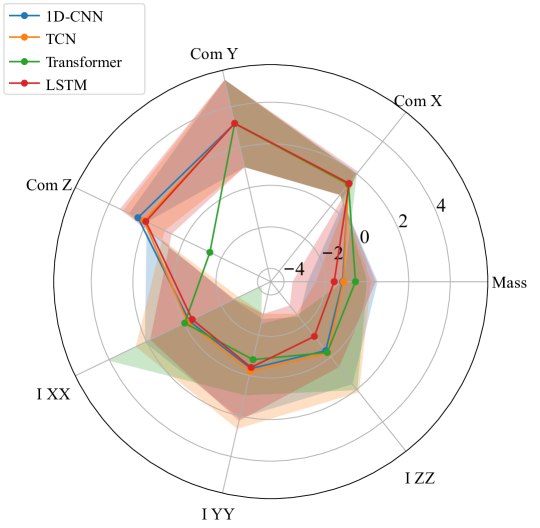
Figure 3: Estimation performance comparison between different time-series data-driven models.

VII CONCLUSION

In this paper, a learning-based estimation for identifying the inertial parameter of an unknown object is proposed. A novel sim-to-real adaptation method combining the Robot System Identification and the Gaussian Processes is introduced to facilitate the seamless transition of a trained learning-based estimator from a simulation to the real world. Our method doesn’t need an additional torque/force sensor, a vision system, and even prior knowledge of the object (e.g., shape). We anticipate our method will boost the performance of collaborative robots, such as manipulators and humanoids, by enabling real-time object dynamics estimation in uncontrolled environments.

VIII Acknowledgements

The authors are grateful to Amartya Purushottam, Youngwoo Sim, and Guillermo Colin for their collaboration through out this work.

References

- [1] A. Purushottam, Y. Jung, K. Murphy, D. Baek, and J. Ramos, “Hands-free telelocomotion of a wheeled humanoid,” in 2022 IEEE/RSJ International Conference on Intelligent Robots and Systems (IROS). IEEE, 2022, pp. 8313–8320.
- [2] A. Wang, J. Ramos, J. Mayo, W. Ubellacker, J. Cheung, and S. Kim, “The hermes humanoid system: A platform for full-body teleoperation with balance feedback,” in 2015 IEEE-RAS 15th International Conference on Humanoid Robots (Humanoids). IEEE, 2015, pp. 730–737.
- [3] C. G. Atkeson, C. H. An, and J. M. Hollerbach, “Estimation of inertial parameters of manipulator loads and links,” The International Journal of Robotics Research, vol. 5, no. 3, pp. 101–119, 1986.
- [4] S. Traversaro, S. Brossette, A. Escande, and F. Nori, “Identification of fully physical consistent inertial parameters using optimization on manifolds,” in 2016 IEEE/RSJ International Conference on Intelligent Robots and Systems (IROS). IEEE, 2016, pp. 5446–5451.
- [5] P. M. Wensing, S. Kim, and J.-J. E. Slotine, “Linear matrix inequalities for physically consistent inertial parameter identification: A statistical perspective on the mass distribution,” IEEE Robotics and Automation Letters, vol. 3, no. 1, pp. 60–67, 2017.
- [6] C. Rucker and P. M. Wensing, “Smooth parameterization of rigid-body inertia,” IEEE Robotics and Automation Letters, vol. 7, no. 2, pp. 2771–2778, 2022.
- [7] T. Lee and F. C. Park, “A geometric algorithm for robust multibody inertial parameter identification,” IEEE Robotics and Automation Letters, vol. 3, no. 3, pp. 2455–2462, 2018.
- [8] C. G. Atkeson, C. H. An, and J. M. Hollerbach, “Rigid body load identification for manipulators,” in 1985 24th IEEE Conference on Decision and Control. IEEE, 1985, pp. 996–1002.
- [9] B. Sundaralingam and T. Hermans, “In-hand object-dynamics inference using tactile fingertips,” IEEE Transactions on Robotics, vol. 37, no. 4, pp. 1115–1126, 2021.
- [10] Y. Yu, K. Fukuda, and S. Tsujio, “Estimation of mass and center of mass of graspless and shape-unknown object,” in Proceedings 1999 IEEE International Conference on Robotics and Automation (Cat. No. 99CH36288C), vol. 4. IEEE, 1999, pp. 2893–2898.
- [11] T. Kroger, D. Kubus, and F. M. Wahl, “12d force and acceleration sensing: A helpful experience report on sensor characteristics,” in 2008 IEEE International Conference on Robotics and Automation. IEEE, 2008, pp. 3455–3462.
- [12] A. C. Smith and K. Hashtrudi-Zaad, “Application of neural networks in inverse dynamics based contact force estimation,” in Proceedings of 2005 IEEE Conference on Control Applications, 2005. CCA 2005. IEEE, 2005, pp. 1021–1026.
- [13] N. Yilmaz, J. Y. Wu, P. Kazanzides, and U. Tumerdem, “Neural network based inverse dynamics identification and external force estimation on the da vinci research kit,” in 2020 IEEE International Conference on Robotics and Automation (ICRA). IEEE, 2020, pp. 1387–1393.
- [14] Z. Lao, Y. Han, Y. Ma, and G. S. Chirikjian, “A learning-based approach for estimating inertial properties of unknown objects from encoder discrepancies,” IEEE Robotics and Automation Letters, 2023.
- [15] T. Standley, O. Sener, D. Chen, and S. Savarese, “image2mass: Estimating the mass of an object from its image,” in Conference on Robot Learning. PMLR, 2017, pp. 324–333.
- [16] C. Diuk, A. Cohen, and M. L. Littman, “An object-oriented representation for efficient reinforcement learning,” in Proceedings of the 25th international conference on Machine learning, 2008, pp. 240–247.
- [17] J. Scholz, M. Levihn, C. Isbell, and D. Wingate, “A physics-based model prior for object-oriented mdps,” in International Conference on Machine Learning. PMLR, 2014, pp. 1089–1097.
- [18] J. Wu, I. Yildirim, J. J. Lim, B. Freeman, and J. Tenenbaum, “Galileo: Perceiving physical object properties by integrating a physics engine with deep learning,” Advances in neural information processing systems, vol. 28, 2015.
- [19] J. Tobin, R. Fong, A. Ray, J. Schneider, W. Zaremba, and P. Abbeel, “Domain randomization for transferring deep neural networks from simulation to the real world,” in 2017 IEEE/RSJ international conference on intelligent robots and systems (IROS). IEEE, 2017, pp. 23–30.
- [20] A. Kumar, Z. Li, J. Zeng, D. Pathak, K. Sreenath, and J. Malik, “Adapting rapid motor adaptation for bipedal robots,” in 2022 IEEE/RSJ International Conference on Intelligent Robots and Systems (IROS). IEEE, 2022, pp. 1161–1168.
- [21] J. Hwangbo, J. Lee, A. Dosovitskiy, D. Bellicoso, V. Tsounis, V. Koltun, and M. Hutter, “Learning agile and dynamic motor skills for legged robots,” Science Robotics, vol. 4, no. 26, p. eaau5872, 2019.
- [22] A. Allevato, E. S. Short, M. Pryor, and A. Thomaz, “Tunenet: One-shot residual tuning for system identification and sim-to-real robot task transfer,” in Conference on Robot Learning. PMLR, 2020, pp. 445–455.
- [23] F. Muratore, C. Eilers, M. Gienger, and J. Peters, “Data-efficient domain randomization with bayesian optimization,” IEEE Robotics and Automation Letters, vol. 6, no. 2, pp. 911–918, 2021.
- [24] Y. Chebotar, A. Handa, V. Makoviychuk, M. Macklin, J. Issac, N. Ratliff, and D. Fox, “Closing the sim-to-real loop: Adapting simulation randomization with real world experience,” in 2019 International Conference on Robotics and Automation (ICRA). IEEE, 2019, pp. 8973–8979.
- [25] Y. Jiang, T. Zhang, D. Ho, Y. Bai, C. K. Liu, S. Levine, and J. Tan, “Simgan: Hybrid simulator identification for domain adaptation via adversarial reinforcement learning,” in 2021 IEEE International Conference on Robotics and Automation (ICRA). IEEE, 2021, pp. 2884–2890.
- [26] A. Purushottam, Y. Jung, C. Xu, and J. Ramos, “Dynamic mobile manipulation via whole-body bilateral teleoperation of a wheeled humanoid,” arXiv preprint arXiv:2307.01350, 2023.
- [27] P. Nadeau, M. Giamou, and J. Kelly, “Fast object inertial parameter identification for collaborative robots,” in 2022 International Conference on Robotics and Automation (ICRA). IEEE, 2022, pp. 3560–3566.
- [28] A. Kumar, Z. Fu, D. Pathak, and J. Malik, “Rma: Rapid motor adaptation for legged robots,” arXiv preprint arXiv:2107.04034, 2021.
- [29] C. E. Rasmussen and C. K. Williams, “Gaussian processes for machine learning, ser. adaptive computation and machine learning,” Cambridge, MA, UsA: MIT Press, vol. 38, pp. 715–719, 2006.
- [30] Y. Wang, R. Gondokaryono, A. Munawar, and G. S. Fischer, “A convex optimization-based dynamic model identification package for the da vinci research kit,” IEEE Robotics and Automation Letters, vol. 4, no. 4, pp. 3657–3664, 2019.
- [31] J. Swevers, C. Ganseman, D. B. Tukel, J. De Schutter, and H. Van Brussel, “Optimal robot excitation and identification,” IEEE transactions on robotics and automation, vol. 13, no. 5, pp. 730–740, 1997.
- [32] V. Makoviychuk, L. Wawrzyniak, Y. Guo, M. Lu, K. Storey, M. Macklin, D. Hoeller, N. Rudin, A. Allshire, A. Handa et al., “Isaac gym: High performance gpu-based physics simulation for robot learning,” arXiv preprint arXiv:2108.10470, 2021.