Energy Management of Hydrogen Hybrid Electric Vehicles - A Potential Study

Abstract

The hydrogen combustion engine (H₂ICE) is known to be able to burn H₂ under ultra-lean conditions, while producing no CO₂ emissions and extremely low engine-out NO${}_{x}^{\mathrm{eo}}$ emissions. This makes the H₂ICE a promising technology for two reasons: Firstly, mid-term goals such as net-zero CO₂ emissions of passenger cars in Europe by 2035 can be achieved. Secondly, immediate goals, as for instance the upcoming EURO 7 NO_x limitations, can be reached more easily as extremely low engine-out NO${}_{x}^{\mathrm{eo}}$ emissions facilitate the reduction of the overall tailpipe NO${}_{x}^{\mathrm{tp}}$ emissions. However, one drawback of the H₂ICE is that for high engine loads, ultra-lean combustion is no longer possible, which partly nullifies its advantage over conventional combustion engines. In this work, the feasibility of achieving consistent reductions in NO${}_{x}^{\mathrm{eo}}$ emissions through the implementation of electric hybridization of an H₂ICE-equipped passenger car (H₂-HEV), combined with a dedicated energy management strategy (EMS) is discussed. In particular, the mixed H₂-HEV architecture is investigated and compared to a series H₂-HEV, a parallel H₂-HEV, and a base H₂-vehicle, which is only equipped with an H₂ICE. For hybrid vehicles, a low H₂ consumption and low NO${}_{x}^{\mathrm{eo}}$ emissions are conflicting objectives, the trade-off of which depends on the EMS and can be represented as a Pareto front. The dynamic programming algorithm is used to calculate the Pareto-optimal EMS calibrations, to display the H₂-NO${}_{x}^{\mathrm{eo}}$ trade-off for various different driving missions. Overall, through the utilization of a dedicated energy management calibration, the mixed H₂-HEV demonstrates the capability to consistently achieve extremely low engine-out NO${}_{x}^{\mathrm{eo}}$ emissions across all investigated driving scenarios. For a broad range of driving missions, the mixed H₂-HEV is able to decrease the engine-out NO${}_{\mathrm{x}}^{\mathrm{eo}}$ emissions by more than 90%, while, at the same time, the H₂ consumption is decreased by over 16%, compared to a comparable non-hybridized H₂-vehicle. These significant emission reductions are possible without having to modify the exhaust-gas aftertreatment system, or the optimization of any of the individual drivetrain components, but solely by setting the EMS calibration accordingly.

organization=Institute for Dynamic Systems and Control,addressline=Sonneggstrasse 3, city=Zürich, postcode=8092, country=Switzerland organization=Robert Bosch GmbH,city=Stuttgard, postcode=70442, country=Germany

1 Introduction

A major challenge of today’s society is to decrease the world-wide CO₂ emissions. In order to support this transition to a cleaner and more sustainable energy future, renewable energies play a critical role [1]. However, with an increasing share of renewable energies, fluctuations in power generation can lead to grid instabilities as energy production does not always align with the current demand. One possibility to cope with the intermittent nature of renewable energies is the use of an energy storage system, which is a carrier that can convert the stored energy back to electric power at any time. Hydrogen energy storage systems are perceived as a relatively inexpensive way of storing, transporting, and trading renewable energies [2], [3].

One major part of the world-wide CO₂ emissions stems from the transportation sector. As in 2022, it was accountable for almost one fourth of the global CO₂ emissions [4], a major part of the global decarbonization politics includes ever more stringent emissions legislations in this sector. In December 2021, the united states environmental protection agency released the final rule [5], setting CO₂ emissions standards to 82.5 g/km for passenger cars until 2026. The European Union has legally regulated the CO₂ emissions of new vehicles to 95 g/km until 2025, to 60 g/km until 2030, and to 0 g/km until 2035 [6]. This signifies the end of the Diesel and gasoline engines’ roles as the dominant technological choices for the light duty market in the EU. However, currently, the traditional combustion engine is still the predominant propulsion technology. In 2019 the global electric-light-vehicles sales accounted for only 2.5% [7]. Therefore, the need to find a replacement for the traditional combustion engine incentivices investments into alternative propulsion technologies that can comply with the net-zero CO₂ goal.

Hydrogen, which results from renewable energies, has long been known to be used as a CO₂-free energy carrier for vehicles. It can be utilized in two ways: Firstly, hydrogen can be used in fuel cells to generate an electric current, which is used to power an electric motor, or stored in a battery. One particular drawback of fuel cells is that they are still rather costly at the moment and require a very high degree of hydrogen purity, since even a low amount of impurity may decrease the fuel cell’s performance and irreversibly shorten its lifespan [8]. Secondly, hydrogen can be directly burned in a hydrogen combustion engine (H₂ICE). The following sections present a literature review that discusses the possibility of H₂ICEs to meet future emission regulations, and explores the options to fill the gap, which will be left by conventional combustion engines.

1.1 Literature Review on H₂ICE

With the increasing focus on hydrogen as a clean and sustainable energy source, coupled with the necessity to explore alternatives to conventional combustion engines, the H₂ICE has emerged as a promising technology for the future. Authors like Shinde et. al. [9], or Falfari et. al. [10] even propose the H₂ICE as the most immediate solution for the near future, as one of its main attractivenesses is that it takes advantage of the current advanced state of ICE technologies. This includes for instance the reliability and durability of combustion engines. Onorati et. al. [11] argue that the H₂ICE can serve, not only as a temporary fast-transition solution, but also as a long-term solution: They emphasize that already existing supply chains and manufactures, plus the already present recycling infrastructure, make the H₂ICE a widespread solution to accelerate the large-scale introduction of H₂ICEs into the transportation market. The transferability of knowledge from conventional combustion engines was demonstrated in multiple publications: The authors of [12] review the applicability of H₂ as a fuel for traditional internal combustion engines and conclude that it can be used in both spark ignition as well as compression ignition engines without any major modifications to the system. Additionally, in [13] the adaption of a single cylinder gasoline engine is described for hydrogen combustion and a peak efficiency of up to 47% could be achieved, highlighting the technology’s excellent combustion efficiency.

For H₂ICEs to be considered a viable future propulsion system, they must also demonstrate compliance with forthcoming greenhouse gas emissions regulations. The new EURO 7 norm for light-duty vehicles is to be expected to become effective in 2025 and includes a fuel-neutral limit for tailpipe NO_x emissions (from now on abbreviated with NO${}_{\mathrm{x}}^{\mathrm{tp}}$) of 60 mg/km [14]. Hydrogen internal combustion engines have long been known for the ability to burn hydrogen with extremely low engine-out NO_x emissions (from now on abbreviated with NO${}_{x}^{\mathrm{eo}}$) [15]. Different strategies are known to achieve such low NO${}_{x}^{\mathrm{eo}}$ emissions during the combustion process of hydrogen. One way is to decrease the combustion temperature, which can be achieved for instance by exhaust gas recirculation (EGR) where already burnt gases are fed back and used in the next combustion. Heffel presents in [16], [17] the use of EGR to reduce the NO${}_{x}^{\mathrm{eo}}$ formation of an H₂ICE. Although he could show that the NO${}_{x}^{\mathrm{eo}}$ formation can be pushed below 10 ppm under stoichiometric conditions, most new publications discuss to exploit the wide flammability range of H₂ to reduce NO${}_{x}^{\mathrm{eo}}$ emissions. This characteristic allows to burn hydrogen using a large surplus of air to decrease the combustion temperature, which is known as ultra-lean combustion. Multiple groups have reported extremely low NO${}_{x}^{\mathrm{eo}}$ emissions using air-to-fuel ratios up to $\lambda\approx 3$. Bao et. al. [18] show that the utilization of a turbocharger and improved injection pressure increase the H₂ICE’s power and efficiency simultaneously. This way they show that extremely low NO${}_{x}^{\mathrm{eo}}$ emissions can be reached with a maximum brake thermal efficiency of 40.4%; Sementa et. al. [19] investigated different H₂ dilutions in experiments and achieved stable combustion up to $\lambda=3.4$, presenting no CO emissions, very low HC emissions, originating from the lubricant oil, and extremely low NO${}_{x}^{\mathrm{eo}}$ emissions.

Whereas ultra-lean combustion can result in excellent emission characteristics, it also has the major drawback of a limited power density compared to stoichiometric or rich combustion conditions. To achieve a high engine power output, increasingly more H₂ has to be injected, which ultimately leads to a lower air-to-fuel ratio. Two issues are to be expected in this situation: Firstly, since ultra-lean combustion is not possible anymore, increasing NO${}_{x}^{\mathrm{eo}}$ emissions will occur, partly nullifying the H₂ICE’s advantage over conventional combustion engines. Secondly, at lower air-to-fuel ratios, H₂ICEs are known to exhibit combustion irregularities such as spontaneous ignition, or knocking [10]. This can be challenging for day-to-day applications in a car, as high engine-load operations are commonly encountered, e.g., acceleration in urban areas, or high-speed driving on the highway. However, if such a vehicle would additionally be equipped with a secondary torque source, e.g., an electric motor, theoretically, both issues could be tackled by assisting the H₂ICE during high engine-loads. In the following, the so-called energy management system (EMS) for hybrid electric vehicles (HEVs) is explained and (if handled properly) its positive effect on reducing the emissions is outlined. Additionally, a summary of the existing literature on HEVs that use an H₂ICE is presented.

1.2 Hybrid Electric Vehicles

The EMS is a necessary control algorithm for every HEV and stems from the fact that any HEV has more than one source to produce power. The EMS is concerned about the provision of the so-called driver’s power request, which is (given the vehicle speed and road inclination) a consequence of the driver’s desired vehicle acceleration. Assuming for instance that the driver demands 20 kW, it remains ambiguous whether this power should originate from the combustive part, the electric part, or a combination of both. This decision of the power allocation is referred to as the power split. Sciaretta et. al have shown in [20] the importance of an elaborate EMS algorithm. The authors compared nine different EMS algorithms for the same vehicle and reported that the best algorithm decreased the overall CO₂ emissions by 28%.
Early approaches for the EMS were of heuristic nature, i.e., they consist of rules which are based on expert’s experience to decide the power split. State-of-the-art algorithms often are based on solving an optimization problem, which results of a mathematical description of the power allocation problem. Such optimization problems are called optimal control problems (OCPs) and include the formulation of mathematical constraint functions, which describe the HEV powertrain sufficiently well, and one (or possibly more) quality criterion for each realizable distribution of the power request. Typical quality criteria would be to achieve minimal CO₂ emissions (e.g. [21]), or the prolongation of battery life (e.g. [22]). The goal of optimization-based EMS algorithms is to find the optimal power split by solving such an OCP using dedicated mathematical solvers.
Overall, EMS control algorithms can be divided into two distinctively different categories, i.e., online controllers, and offline algorithms. Online controllers are designed such that they can be implemented on the vehicle’s embedded control unit. They are causal, meaning that all signals necessary for calculating the controller outputs are accessible at the instance of the computation process. Here, the main challenges are to achieve a good trade-off between computing a power split, which leads to acceptable CO₂ emissions, and complying with the restrictions of the embedded hardware on the vehicle. Offline EMS algorithms, however, are simulative investigations of the potential of the HEV’s fuel saving capabilities. They are often described as non-causal, meaning that they have access to all constraints and disturbances of the OCP at each point in time. Here, the goal is to find the theoretically best possible solution to the OCP, which describes finding the HEVs optimal power split at every point in time for a predefined driving mission. Although such investigations cannot capture all effects that occur during real-world driving, they are a valuable tool to investigate the impact of different powertrain topologies on the achievable performance in simulation before building the physical system.

One well-known extension of the energy management problem includes the NO_x emissions. As a result, a typical multi-objective optimization problem is obtained, which means that the OCP includes two competing objectives, namely: the minimization of CO₂ emissions, and the minimization of NO_x emissions. Since these objectives are in conflict, such OCPs do not have one single optimal solution anymore, but a multitude of solutions that lie on the so-called Pareto front. Each solution on this Pareto front is a different optimal realization of the fuel-NO_x trade-off, i.e., reducing CO₂ always comes at the expense of increasing NO_x, and vice-versa. Using offline algorithms, Ritzmann et. al. have investigated the fuel-NO_x trade-off potential of a parallel HEV that is equipped with a Diesel engine, and compared it to a non-electrified vehicle [23]. They have shown that for a comparable fuel consumption, the NO${}_{\mathrm{x}}^{\mathrm{tp}}$ can roughly be halved by using the hybrid propulsion technology. Moreover, the fuel-NO_x trade-off that results from different choices of the EMS controller design, spans a wide range.

Although the literature is rich in examples for experiments addressing HEVs that are equipped with either a Diesel engine or a gasoline engine, there are only few reports on vehicles that use hydrogen combustion as part of their HEV architecture (from herein on referred to as H₂-HEV). The only two test vehicles presented in the literature are as follows: In [24], a standard sport utility vehicle has been converted into a hydrogen-powered H₂-HEV. In [25], a hydrogen engine propelled hybrid electric concept vehicle, called Ford’s H₂RV, is described. In both studies, the authors state excellent NO${}_{\mathrm{x}}^{\mathrm{tp}}$ emissions while achieving low H₂ consumption. However, the achieved results would not satisfy the future legislation limitations that are expected with the introduction of, e.g., EURO 7. Two reasons can be identified for the relatively high NO${}_{\mathrm{x}}^{\mathrm{tp}}$ emissions: Firstly, both studies are based on old examples of vehicles (2006 and 2004). Secondly, both vehicles were equipped with EMS algorithms that are inferior to todays state-of-the-art methods, which can have a substantial influence on the fuel-NO_x trade-off (from now on referred to as the H₂-NO_x trade-off).

Only two publications are found in the literature regarding the simulative performance of an H₂-HEV that is equipped with a modern turbocharged H₂ICE. The first publication, written by Beccari et. al. [26], compares the CO₂ emissions of a standard HEV with a Diesel engine to an H₂-HEV. Although not elaborated in detail, the authors simply describe to operate the combustion engine in its optimal operating point at each point in time. However, this does neither explain how the electrical components are operated, nor are any effects on the battery energy content shown and discussed. Additionally, the NO_x emissions are not taken into consideration and the investigations are limited to one driving cycle.
The second publication, written by Kyjovský et. al. [27], compares the CO₂ and NO_x emissions of parallel H₂-HEVs from different weight classes on the WLTC in simulation. They report good fuel consumption, while the lighter vehicles show NO_x emissions below the limits imposed by EURO 6, without the use of an aftertreatment system. As the main focus of this publication lies in the investigation of turbocharging and engine downsizing, the EMS plays a subordinated role. Therefore, instead of computing the entire realizable Pareto front, a standard EMS algorithm is implemented, which results in a sub-optimal vehicle performance. As a result, the approach presented has two major shortcomings: Firstly, no measure is given of how much CO₂ (or NO_x, respectively) can be saved using a theoretically optimal EMS controller. Secondly, without the full Pareto front, it is impossible to know how much either of these two quantities could have been reduced at the expense of the other.

1.3 Contribution

In this publication, a simulative comparison between three different H₂-HEV architectures and a base H₂-vehicle, which is only equipped with an H₂ICE, is conducted. The different hybrid propulsion architectures feature a series H₂-HEV, a parallel H₂-HEV, and a mixed H₂-HEV. The contribution of this publication is twofold.

1. To the authors’ best knowledge, for the first time, this publication presents the full performance potential that is achievable by an optimal EMS calibration on different H₂-HEVs. This includes the entire achievable trade-off between H₂ consumption and engine-out NO${}_{\mathrm{x}}^{\mathrm{eo}}$ emissions. These H₂-NO${}_{\mathrm{x}}^{\mathrm{eo}}$ Pareto fronts are obtained with the dynamic programming algorithm (DP), which guarantees global optimality for a predefined driving mission. A comparison on the WLTC reveals that all hybrid propulsion architectures outperform the non-hybridized H₂ICE, whereas the mixed H₂-HEV is superior over the series and the parallel configuration.

2. To solidify the findings, the achievable trade-off between H₂ consumption and engine-out NO${}_{\mathrm{x}}^{\mathrm{eo}}$ emissions of the mixed H₂-HEV is presented for a wide variety of driving missions. An in-depth analysis of different realizations of H₂-NO${}_{\mathrm{x}}^{\mathrm{eo}}$-optimal solutions provides insight into how the mixed H₂-HEV architecture can be exploited to operate the H₂ICE solely under ultra-lean conditions, resulting in extremely low NO${}_{\mathrm{x}}^{\mathrm{eo}}$ emissions. Consequently, two worst-case driving scenarios are analyzed to highlight the technical limitations of the mixed H₂-HEV. In conclusion, to the authors’ best knowledge, this study provides the first complete overview of the potential of H₂-HEVs to satisfy future emission legislations, solely via the optimal calibration of the EMS algorithm.

The remainder of this paper is organized as follows: In Section 2, the different H₂-HEV models are outlined and the energy management problem including NO${}_{\mathrm{x}}^{\mathrm{eo}}$ emissions is formulated as an OCP. In Section 3, a comparison between the performance of the different H₂-HEVs and the base H₂-vehicle is presented on the WLTC. Furthermore, with regards to the H₂-NO${}_{\mathrm{x}}^{\mathrm{eo}}$ trade-off, the benefits of hybridization over only using an H₂ICE are discussed and the superiority of the mixed H₂-HEV is explained. In Section 4, the achievable H₂-NO${}_{\mathrm{x}}^{\mathrm{eo}}$ trade-off of the mixed H₂-HEV is presented for four additional driving missions, including two worst-case driving scenarios, highlighting the technology’s limitations. In Section 5, an outlook on future research is presented.

2 Problem Description

In this section, the four investigated drivetrain configurations are introduced. Firstly, the base H₂-vehicle is explained, then the three hybridized H₂-HEVs are presented. Subsequently the energy management problem including NO${}_{\mathrm{x}}^{\mathrm{eo}}$ emissions is outlined.

2.1 Drivetrain Configurations

For the sake of comparison, the investigated H₂-HEVs are built upon the base H₂-vehicle, but with additional electrical components. This ensures uniformity across the analyzed vehicles with respect to the H₂ICE, aerodynamic drag and rolling resistance, and the base H₂-vehicle’s mass $m_{\mathrm{base}}$. The H₂-HEVs have additional weight, according to their individual electrical equipment. Table 1 summarizes the individual vehicle parameters. Note that the vehicle components are additive, meaning that, if, e.g., the series H₂-HEV is considered, then it also includes the components of the base H₂-vehicle and the parallel H₂-HEV.

For all investigated propulsion architectures, the engine ON/OFF state is described by the binary variable $e_{0}$ and the clutch state (if a clutch is included) is described by the binary variable $c_{0}$. While a value of $e_{0}=1$ indicates that the engine is running, $e_{0}=0$ indicates that it is turned off. Regarding the clutch, $c_{0}=1$ indicates that the clutch is engaged, while $c_{0}=0$ indicates that the clutch is open.

Base vehicle:
Figure 1 shows a schematic of the powertrain architecture of the base H₂-vehicle and electric parts in gray. The electric parts are only used in the parallel H₂-HEV drivetrain and are introduced in a section further down.

Figure 1: Schematic of the base H₂-vehicle and the parallel H₂-HEV. The components that are grayed out are only part of the parallel H₂-HEV.

The H₂ICE is connected to the front axle through a seven speed gearbox, the clutch, and a differential. The seven speed gearbox’s transmission ratios are denoted by $\gamma_{\mathrm{e,1-7}}$. As for this vehicle the only power source is the H₂ICE, any positive torque request of the driver has to be supplied by the H₂ICE. If the torque request is negative, or zero, then the clutch is opened ($c_{0}=0$), the engine is shut-off ($e_{0}=0$), and the friction brakes are used. As a result, engine idling is prevented. Engine braking is not considered in this work.

Parallel H₂-HEV:
The parallel H₂-HEV propulsion architecture results from adding the electrical parts that are grayed out in Figure 1. A torque split device, which is denoted by $q$, is used before the gearbox, resulting in a P3 hybrid. The additional electric motor uses the fixed-gear transmission $\gamma_{\mathrm{mot}}$ and can draw power from or feed power to the battery. In addition to the base weight of the vehicle, the electric devices account for $m_{\mathrm{e,par}}=160$ kg, which includes the battery, an electric motor, and power electronics.

Series H₂-HEV:
Figure 2 shows a schematic of the powertrain architecture of the series H₂-HEV and grayed out parts. The grayed out clutch, fixed gearbox, and torque split device are used in the mixed H₂-HEV drivetrain and are introduced in a section further down. The H₂ICE is not physically connected to the wheels, but is only used to produce electric energy via the generator. This electric energy is either directly used by the motor, fed to the battery, or employed in both ways simultaneously. The motor and the generator are the same make and model, whereas the motor has the same fixed transmission ratio as in the parallel H₂-HEV, and the generator has a different fixed transmission ratio $\gamma_{\mathrm{gen}}$. In addition to the base weight of the vehicle, the electric devices account for $m_{\mathrm{e,ser}}=200$ kg, which includes the battery, the electric motor, the generator, and power electronics.

Figure 2: Schematic of the base series H₂-HEV and the mixed H₂-HEV. The components grayed out are only part of the mixed H₂-HEV.

Mixed H₂-HEV:
The mixed H₂-HEV propulsion architecture results from adding the parts in Figure 2 that are grayed out. The clutch can be used to connect the H₂ICE to the wheels via a fixed transmission $\gamma_{\mathrm{e,mix}}$ and the torque split device $q$. This drivetrain architecture is called mixed H₂-HEV, since it combines a series H₂-HEV and a parallel H₂-HEV architecture. In addition to the base weight of the vehicle, the electric devices account for $m_{\mathrm{e,mix}}=200$ kg, which includes the battery, the electric motor, the generator, and power electronics.

Driving modes:
Hybrid electric vehicles encompass various driving modes that arise from the flexibility to either use multiple power sources simultaneously, or to rely on only one power source and to decouple, or switch off, the other one(s). The different driving modes are denoted by $M\in\{1,2,3\}$ in this work, and are listed in Table 2. In series mode, the H₂ICE is running, but it is decoupled from the wheels, i.e., any requested power is fully delivered by the motor. In parallel mode, the H₂ICE is running and physically coupled to the wheels. In this mode, both propulsion systems (H₂ICE and motor) can provide power to the wheels. It also enables load-point shifting, where the combustion engine produces more power than is required at the wheels and the access power is stored in the battery. In EV mode, the combustion engine is off and decoupled from the wheels. The entire torque request is met by the motor.

Table 1: Vehicle parameters of the four propulsion architectures.

base H2-vehicle	weight	1300 kg
	H2ICE	4-cyl
		163 kW
parallel H2-HEV	motor	173 kW
		40 kg
	battery	230 V
		11 kWh
		120 kg
series- & mixed H2-HEV	generator	173 kW
		40 kg

Table 2: Driving modes of the different propulsion architectures.

Series mode	$c_{0}=0$, $e_{0}=1$	$M=1$
Parallel mode	$c_{0}=1$, $e_{0}=1$	$M=2$
EV mode	$c_{0}=0$, $e_{0}=0$	$M=3$

2.2 Drivetrain Model

The modeling approach used in this work is based on [28] and is outlined in the following.

Propulsion systems:
The engine’s fuel consumption and the NO${}_{\mathrm{x}}^{\mathrm{eo}}$ emissions are obtained using steady-state mappings that were evaluated on a test bench and depend on the engine speed $\omega_{e}$ and the engine torque $T_{e}$:

$$\dot{m}_{f} =f(\omega_{e},T_{e})$$ (1)

$$\dot{m}_{\mathrm{NO}_{\mathrm{x}}} =f(\omega_{e},T_{e}).$$ (2)

The obtained maps are depicted in Figure 3. Extremely low NO${}_{\mathrm{x}}^{\mathrm{eo}}$ can be reached under low-load conditions. This is possible as the turbocharged H₂ICE is calibrated to operate under ultra-lean combustion conditions in this region, leading to NO${}_{\mathrm{x}}^{\mathrm{eo}}$ emissions below 2 mg/s.

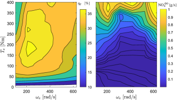
Figure 3: Left: H₂ICE efficiency map. Right: NO${}_{\mathrm{x}}^{\mathrm{eo}}$ map.

The electric motor and generator losses are stored in maps that are derived from high-fidelity component models:

$$P_{\mathrm{l}_{\mathrm{mot}}}=f(T_{\mathrm{mot}},\omega_{\mathrm{mot}}),$$ (3)

$$P_{\mathrm{l}_{\mathrm{gen}}}=f(T_{\mathrm{gen}},\omega_{\mathrm{gen}}).$$ (4)

They depend on the torque and the rotational speed of the corresponding component. Their efficiency maps are depicted in Figure 4.

Figure 4: Left: Generator efficiency map. Right: Motor efficiency map. Motor and generator are of the same make and model.

Torque request:
The requested force at the wheels is a function of the aerodynamic drag force and rolling resistance $F_{d}$, the gravitational force $F_{g}$, and the inertial force $F_{i}$ to accelerate the vehicle:

$$F_{\mathrm{req}}=F_{d}(v)+F_{g}(\Gamma)+F_{i}(a),$$ (5)

where $\Gamma$ denotes the road gradient, $v$ the velocity, and $a$ the vehicle acceleration. The resistive force $F_{d}$ is approximated using a quadratic dependency on $v$. The inertial force $F_{i}$ is calculated by accelerating the total mass of the vehicle $m_{\mathrm{tot}}$:

$$F_{i} =m_{\mathrm{tot}}\cdot a,$$ (6)

$$m_{\mathrm{tot}} =\begin{cases}m_{\mathrm{base}}+m_{\mathrm{e,par}}&\text{,if parallel H${}_{2}$-HEV},\\ m_{\mathrm{base}}+m_{\mathrm{e,ser}}&\text{,if series H${}_{2}$-HEV},\\ m_{\mathrm{base}}+m_{\mathrm{e,mix}}&\text{,if mixed H${}_{2}$-HEV},\end{cases}$$

where $m_{\mathrm{e,}j},j\in\{\mathrm{par},\mathrm{ser},\mathrm{mix}\}$ accounts for the sum of all additional electric devices that make up the hybridized versions of the base H₂-vehicle. The resulting torque request is calculated using the wheel’s radius $r_{w}$:

$$T_{\mathrm{req}}=F_{\mathrm{req}}\cdot r_{w}.$$ (7)

The torque request has to be provided by the vehicle’s combined drivetrain. For the case of the base H₂-vehicle, the entire torque is delivered by the H₂ICE, which means that the H₂ consumption and NO${}_{\mathrm{x}}^{\mathrm{eo}}$ emissions can directly be calculated using (1) and (2). For the case of the H₂-HEVs, the torque request can be divided between multiple power sources at each point in time. This power distribution is explained in the following for the mixed H₂-HEV. However, the torque splits for the parallel H₂-HEV and the series H₂-HEV can directly be obtained from the same description.

Rotational Speeds:
Before the torque split is introduced, the description of the rotational speeds of the mixed H₂-HEV components are explained. From the vehicle speed, the wheel speed calculates as:

$$\omega_{w}=\frac{v}{r_{w}}.$$ (8)

As the motor is always physically coupled to the wheels, its speed is directly defined by:

$$\omega_{\mathrm{mot}}=\omega_{w}\cdot\gamma_{\mathrm{fd}}\cdot\gamma_{\mathrm{mot}},$$ (9)

whereas $\gamma_{\mathrm{fd}}$ and $\gamma_{\mathrm{mot}}$ are the fixed gear ratios of the final drive, and the motor, respectively. The engine is not always physically coupled to the wheels, as this connection depends on the driving mode. If the vehicle is in parallel mode, $\omega_{\mathrm{e}}$ is defined by the wheel speed and the respective engine transmission ratio $\gamma_{e,i}$. The engine transmission is different for the individual vehicles, which is here denoted by the subscript $i\in\{\mathrm{mix},\mathrm{1-7}\}$. The mixed H₂-HEV’s gear ratio $\gamma_{\mathrm{e,mix}}$ is fixed, whereas for the base H₂-vehicle and for the parallel H₂-HEV, $\gamma_{\mathrm{e,1-7}}$ is defined by the seven-speed gearbox, which again is encoded via the vehicle speed. However, if the vehicle is in series mode, or in EV mode, then the clutch is open and $\omega_{\mathrm{e}}$ is defined by the generator speed $\omega_{\mathrm{gen}}$:

$$\omega_{\mathrm{e}}=\begin{cases}\omega_{w}\cdot\gamma_{\mathrm{fd}}\cdot\gamma_{\mathrm{e,i}}&\text{,if $M=2$},\\ \frac{\omega_{\mathrm{gen}}}{\gamma_{\mathrm{gen}}}&\text{,if $M\in\{1,3\}$},\end{cases}$$ (10)

whereas $\gamma_{\mathrm{gen}}$ is the fixed gear ratio of the generator.

Similar to the engine speed, the generator speed depends on the driving mode. In parallel mode, $\omega_{\mathrm{gen}}$ is fixed by the vehicle speed. In EV mode, the generator is switched off by design and its rotational speed is zero. In series mode, the generator speed can be chosen freely and does not depend on the vehicle speed.

$$\omega_{\mathrm{gen}}=\begin{cases}\in[\omega_{\mathrm{gen}}^{\mathrm{min}},\,\omega_{\mathrm{gen}}^{\mathrm{max}}]&\text{,if $M=1$},\\ \omega_{w}\cdot\gamma_{\mathrm{fd}}\cdot\gamma_{\mathrm{gen}}&\text{,if $M=2$},\\ 0&\text{,if $M=3$}.\end{cases}$$ (11)

Here, $\omega_{\mathrm{gen}}^{\mathrm{min}}$ and $\omega_{\mathrm{gen}}^{\mathrm{max}}$ represent physical limits implied by the engine idle speed and the engine max speed.

Torque Split:
After all rotational speeds are defined, the torque split for the mixed H₂-HEV can be formulated. Including the efficiency of the final drive $\eta_{\mathrm{fd}}$, the torque request is calculated before the torque split device as:

$$T_{\mathrm{req}_{\mathrm{fd}}}=\begin{cases}\nicefrac{{T_{\mathrm{req}}}}{{\gamma_{\mathrm{fd}}}}\div\eta_{\mathrm{fd}}&\text{,if $T_{\mathrm{req}}\geq 0$},\\ \nicefrac{{T_{\mathrm{req}}}}{{\gamma_{\mathrm{fd}}}}\,\cdot\,\eta_{\mathrm{fd}}&\text{,if $T_{\mathrm{req}}<0$}.\end{cases}$$ (12)

Considering the motor gearbox efficiency $\eta_{\mathrm{GB}_{\mathrm{mot}}}$, the torque split device $q$ is used to distribute $T_{\mathrm{req}_{\mathrm{fd}}}$ between the electric motor torque:

$$T_{\mathrm{mot}_{\mathrm{req}}} =T_{\mathrm{req}_{\mathrm{fd}}}\cdot q,$$ (13)

$$T_{\mathrm{mot}} =\begin{cases}\frac{T_{\mathrm{mot}_{\mathrm{req}}}}{\gamma_{\mathrm{mot}}}\div\eta_{\mathrm{GB}_{\mathrm{mot}}}&\text{,if $T_{\mathrm{req}_{\mathrm{fd}}}\geq 0$},\\ \frac{T_{\mathrm{mot}_{\mathrm{req}}}}{\gamma_{\mathrm{mot}}}\,\cdot\,\eta_{\mathrm{GB}_{\mathrm{mot}}}&\text{,if $T_{\mathrm{req}_{\mathrm{fd}}}<0$},\end{cases}$$

and the torque that is requested from the combined engine-generator-unit:

$$T_{e_{\mathrm{req}}}=T_{\mathrm{req}_{\mathrm{fd}}}\cdot(1-q).$$ (14)

In series mode and in EV mode, the full power is delivered by the motor. But in parallel mode, the torque split can be chosen arbitrarily as long as the torque distribution can be delivered by the corresponding components. Therefore, the possible choice of torque splits is defined as:

$$q=\begin{cases}1&\text{,if $M\in\{1,\,3\}$}\\ ]-\infty,\infty[&\text{,if $M=2$}.\end{cases}$$ (15)

As the generator and the engine are physically coupled, the final torque, which the engine has to deliver, is defined by the generator gearbox efficiency $\eta_{\mathrm{GB}\mathrm{gen}}$ and the generator torque:

$$T_{e}=T_{e_{\mathrm{req}}}-\frac{T_{\mathrm{gen}}\cdot\gamma_{\mathrm{gen}}}{\eta_{\mathrm{GB}\mathrm{gen}}}.$$ (16)

Similar to the torque split, the choice of obtainable generator torques depends on the driving mode:

$$T_{\mathrm{gen}}=\begin{cases}[T^{\mathrm{min}},\,T^{\mathrm{max}}]&\text{$M\in\{1,\,2\}$}\\ 0&\text{$M=3$}.\end{cases}$$ (17)

The torque bounds $T^{\mathrm{min}}$ and $T^{\mathrm{max}}$ represent the torque limits of the combined engine-generator unit. Finally, to calculate the electric power that is drawn from the battery, the source power that is provided by the motor and generator calculates as:

$$P_{\mathrm{mot}_{\mathrm{s}}}=T_{\mathrm{mot}}\cdot\omega_{\mathrm{mot}}+P_{\mathrm{l}_{\mathrm{mot}}},$$ (18)

and

$$P_{\mathrm{gen}_{\mathrm{s}}}=T_{\mathrm{gen}}\cdot\omega_{\mathrm{gen}}+P_{\mathrm{l}_{\mathrm{gen}}}.$$ (19)

The battery is modeled using a Thévenin equivalent model [28]. The current $I_{b}$ and that results from a requested battery power $P_{b}$ calculates as

$$I_{b} =\frac{V_{oc}-\sqrt{V_{oc}^{2}-4R_{i}P_{b}}}{2R_{i}},$$ (20)

$$P_{b} =P_{\mathrm{mot}_{\mathrm{s}}}+P_{\mathrm{gen}_{\mathrm{s}}}+P_{\mathrm{aux}},$$

where the inner resistance $R_{i}$ and the auxiliary losses $P_{\mathrm{aux}}$ are assumed to be constant. The battery source power calculates as

$$P_{s_{b}} =P_{b}+P_{l_{b}},$$ (21)

$$P_{l_{b}} =R_{i}\cdot I_{b}^{2},$$

where the battery internal losses are denoted by $P_{\mathrm{l}_{b}}$. The high-voltage battery open circuit voltage $V_{\mathrm{oc}}$ can be approximated to depend linearly on the state of charge (SoC) [29] and is described in this work as:

$$V_{\mathrm{oc}}=\alpha_{\mathrm{bat}}\cdot\mathrm{SoC}+\beta_{\mathrm{bat}},$$ (22)

where $\alpha_{\mathrm{bat}}$, $\beta_{\mathrm{bat}}$ are fitted parameters. The battery SoC dynamics are described by:

$$\dot{\mathrm{SoC}} =\frac{-P_{s_{b}}}{Q_{\mathrm{max}}\cdot V_{\mathrm{oc}}},$$ (23)

where $Q_{\mathrm{max}}$ is the full battery capacity.

Overall, the above introduced torque split description is valid for the mixed H₂-HEV architecture. However, the torque splits for the series H₂-HEV and the parallel H₂-HEV are obtained by choosing the corresponding parts of (10), (11), (15), and (17).

2.3 Energy Management Including NO${}_{\mathrm{x}}^{\mathrm{eo}}$:

To formulate the optimal control problem of the energy management including NO${}_{\mathrm{x}}^{\mathrm{eo}}$, the vector of dynamic state variables and its derivative are defined as:

$$\mathbf{x} =[\mathrm{SoC},\,m^{\mathrm{eo}}_{\mathrm{NO}_{\mathrm{x}}}]^{T},$$ (24)

$$\mathbf{\dot{x}} =[\dot{\mathrm{SoC}},\,\dot{m}^{\mathrm{eo}}_{\mathrm{NO}_{\mathrm{x}}}]^{T}=\mathbf{f}(\mathbf{x},\mathbf{u}).$$

Here, the accumulated and instantaneous NO${}_{\mathrm{x}}^{\mathrm{eo}}$ emissions are denoted by $m^{\mathrm{eo}}_{\mathrm{NO}_{\mathrm{x}}}$, and $\dot{m}^{\mathrm{eo}}_{\mathrm{NO}_{\mathrm{x}}}$, respectively. The variable $\mathbf{u}$ represents the vector of control inputs, which depends on the investigated vehicle. The most general case is for the mixed H₂-HEV, as this architecture offers all degrees of freedom to manipulate the torque split. It is defined as:

$$\mathbf{u}=[T_{\mathrm{gen}},\,\omega_{\mathrm{gen}},\,q,\,M]^{T}.$$ (25)

The base H₂-vehicle and the remaining H₂-HEVs use a subset of $\mathbf{u}$. Table 3 lists an overview of the sets of control inputs for all investigated vehicles.

Table 3: Overview of the degrees of freedom of the investigated propulsion architectures.

	$T_{\mathrm{gen}}$	$\omega_{\mathrm{gen}}$	$q$	$M$
Base H2-vehicle	$\times$	$\times$	$\times$	$\times$
Parallel H2-HEV	$\times$	$\times$	$\checkmark$	$\{2,\,3\}$
Series H2-HEV	$\checkmark$	$\checkmark$	$\times$	$\{1,\,3\}$
Mixed H2-HEV	$\checkmark$	$\checkmark$	$\checkmark$	$\{1,\,2,\,3\}$

The goal of solving the optimal control problem of the energy management including NO${}_{\mathrm{x}}^{\mathrm{eo}}$ emissions (from here on referred to as OCP) is to find the optimal power distribution for a predefined driving mission, such that the H₂ consumption is as low as possible, while the NO${}_{\mathrm{x}}^{\mathrm{eo}}$ emissions are kept below an upper limit $\bar{m}^{\mathrm{eo}}_{\mathrm{NO}_{\mathrm{x}}}$. The OCP is written in time domain, i.e., the driving mission starts at the time instance $t_{0}$ and ends at time instance $t_{f}$. The vehicle has to be operated in charge-sustaining mode, i.e., the SoC must be the same at the end and at the start of the driving mission. Using the definitions for $\mathbf{x}$, $\mathbf{u}$, and equations $(\ref{eq:omega_w})$ – $(\ref{eq:Voc})$ as constraints, the OCP is written as follows:

$$\underset{\mathbf{u}}{\text{min}}\quad\quad\, \int_{t_{0}}^{t_{\text{f}}}\dot{m}_{f}\,dt$$ (26a)

$$\text{ \qquad s.t.}\quad T_{\mathrm{req}_{\mathrm{fd}}} =T_{e_{\mathrm{req}}}+T_{\mathrm{mot}_{\mathrm{req}}}$$ (26b)

$$\dot{\mathrm{SoC}} =f(\mathbf{x},\mathbf{u})$$ (26c)

$$\dot{m}^{\mathrm{eo}}_{\mathrm{NO}_{\mathrm{x}}} =f(\mathbf{u})$$ (26d)

$$\mathrm{SoC}(t_{0}) =0.7$$ (26e)

$$\mathrm{SoC}(t_{f}) =0.7$$ (26f)

$$m^{\mathrm{eo}}_{\mathrm{NO}_{\mathrm{x}}}(t_{0}) =0$$ (26g)

$$m^{\mathrm{eo}}_{\mathrm{NO}_{\mathrm{x}}}(t_{f}) \leq\bar{m}^{\mathrm{eo}}_{\mathrm{NO}_{\mathrm{x}}}$$ (26h)

$$\mathbf{u} \in\mathcal{U}$$ (26i)

$$\mathbf{x} \in\mathcal{X}.$$ (26j)

Equation (26b) is called the driveability constraint and ensures that the driver’s torque request is fulfilled. The set of feasible inputs (26i) encompasses the constraints that are defined by (11), (15), (17), as well as, the physical limitations of the drivetrain’s components. The set of feasible state variables (26j) encompasses constant bounds on SoC $\in[0.3,\,0.9]$ and constant bounds on $m^{\mathrm{eo}}_{\mathrm{NO}_{\mathrm{x}}}\in[0,\bar{m}^{\mathrm{eo}}_{\mathrm{NO}_{\mathrm{x}}}]$.

The OCP at hand is a nonlinear mixed-integer optimal control problem. Although, the dynamic programming algorithm (DP) could directly be used to solve the problem with optimality guarantees, the so-called curse of dimensionality [30] hinders its effective applicability. Therefore, a shooting algorithm is exploited to reduce the problem’s dimensionality by eliminating the $m^{\mathrm{eo}}_{\mathrm{NO}_{\mathrm{x}}}$ state without jeopardizing the solution’s global optimality. A slight adaption of the PMP-DP-algorithm that was proposed in [31] is used. A sketch of the idea is outlined in the following: Instead of solving the OCP (26) only for one upper bound $\bar{m}^{\mathrm{eo}}_{\mathrm{NO}_{\mathrm{x}}}$, the cost function (26a) is adjoined with an equivalent fuel consumption weight for the $\dot{m}^{\mathrm{eo}}_{\mathrm{NO}_{\mathrm{x}}}$ emissions, and this resulting adapted optimal control problem is solved multiple times for different weights. On the one hand, adjoining the $\dot{m}_{\mathrm{NO}_{\mathrm{x}}}$ dynamics allows to omit the constraint (26h), which can be leveraged to greatly decrease the computational burden, compared to solving the original OCP with the DP algorithm. On the other hand, this shooting method results in a Pareto front for the H₂-NO${}_{\mathrm{x}}^{\mathrm{eo}}$ trade-off, which will be discussed in the following.

3 Results: WLTC

The performance of the investigated propulsion architectures is analyzed using the results obtained with the adapted PMP-DP algorithm. Depending on the choice of the upper limit $\bar{m}^{\mathrm{eo}}_{\mathrm{NO_{\mathrm{x}}}}$ in (26h), different optimal EMS calibrations are realized for the same driving mission, which results in a Pareto front. All Pareto fronts in this paper are normalized using H_2,0 and NO${}_{\mathrm{x},0}^{\mathrm{eo}}$, which are the H₂ consumption and NO${}_{\mathrm{x}}^{\mathrm{eo}}$ emissions of the base H₂-vehicle, respectively. As for the base H₂-vehicle, no torque split can be optimized, these values are fixed to a corresponding driving mission.

Figure 5 shows the trade-off between the H₂ consumption and the NO${}_{\mathrm{x}}^{\mathrm{eo}}$ emissions for the WLTC. The different hybridized propulsion configurations are shown in yellow, red, and blue for the parallel, series, and mixed H₂-HEV, respectively. Depending on the torque distribution, different H₂ consumptions and NO${}_{\mathrm{x}}^{\mathrm{eo}}$ emissions ensue. From here on, the H₂-optimal EMS calibration of the mixed H₂-HEV will be indicated by $\mathcal{S}^{\star}$ and is depicted by the point farthest to the right of the corresponding Pareto front. The NO${}_{\mathrm{x}}^{\mathrm{eo}}$-optimal EMS calibration of the mixed H₂-HEV will be indicated by $\mathcal{S}^{\blacksquare}$ and is depicted by the point the farthest to the left of the corresponding Pareto front. Each point on the corresponding Pareto front represents a realizable EMS calibration which results in a unique combination of NO${}_{\mathrm{x}}^{\mathrm{eo}}$ emissions and H₂ consumption, demonstrating that a hybridized powertrain architecture opens a large range of realizable trade-offs. To enable a comparative assessment of the individual vehicles, a specific level of accumulated NO${}_{\mathrm{x}}^{\mathrm{eo}}$ emissions is established, and the corresponding hydrogen consumptions of each vehicle are then compared. This concept is graphically represented by the black dashed line. To facilitate below analysis, the intersection of the mixed H₂ HEV’s Pareto front and black dashed line is the EMS calibration denoted by $\mathcal{S}^{--}$.

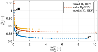
Figure 5: Achievable H₂-NO${}_{\mathrm{x}}^{\mathrm{eo}}$ trade-off for the mixed H₂-HEV, the series H₂-HEV, and the parallel H₂-HEV. The results are normalized using H_2,0 and NO${}_{\mathrm{x},0}^{\mathrm{eo}}$, both of which are obtained by simulations of the base H₂-vehicle. The black, dotted line represents an arbitrary accumulated NO${}_{\mathrm{x},0}^{\mathrm{eo}}$ value and is used for comparison.

3.1 Base vehicle vs mixed H₂-HEV

The blue line depicts the Pareto front, which can be achieved using the mixed H₂-HEV. The EMS calibration, which emits the same NO${}_{\mathrm{x}}^{\mathrm{eo}}$ emissions as the base H₂-vehicle, is located where its x-value equals to one. As a result, this simulation study reveals that for the same NO${}_{\mathrm{x}}^{\mathrm{eo}}$ emissions, an H₂ reduction potential of 16.8% is possible with the use of the mixed H₂-HEV. Even more remarkable is that the realizable NO${}_{\mathrm{x}}^{\mathrm{eo}}$ emissions by the mixed H₂-HEV can be more than one order of magnitude lower than what is achieved by the base H₂-vehicle. This suggests that the base H₂-vehicle cannot be operated under ultra-lean combustion conditions throughout the entire drive mission.

To investigate the base H₂-vehicle’s NO${}_{\mathrm{x}}^{\mathrm{eo}}$ emissions in detail, the operating conditions of its H₂ICE are analyzed below. Figure 6 shows in the upper plot all operating points of the base vehicle in the engine efficiency map and the NO${}_{\mathrm{x}}^{\mathrm{eo}}$ map. Two things can be noted here: Firstly, many operating points lie in the low-load region, which is a well-known issue resulting in a low mean engine efficiency compared to hybrid powertrain configurations. Secondly, the NO${}_{\mathrm{x}}^{\mathrm{eo}}$ map predicts a steep increase in NO${}_{\mathrm{x}}^{\mathrm{eo}}$ production for increased engine torques. Although, most of the engine operating points are located in a region where very low NO${}_{\mathrm{x}}^{\mathrm{eo}}$ emissions occur, some operating points of the base H₂-vehicle lie critically close to the steep region.
To investigate these critical points in detail, the middle plot shows a time-resolved graph of the NO${}_{x,0}^{\mathrm{eo}}$ emitted by the base H₂-vehicle normalized by the NO${}_{\mathrm{x}}^{\mathrm{eo}}$ emitted by $\mathcal{S}^{--}$ of the mixed H₂-HEV. It shows that, most of the time, both vehicles have NO${}_{\mathrm{x}}^{\mathrm{eo}}$ emissions, which have the same order of magnitude. However, the spikes in this signal reveal where the base H₂-vehicle emits substantially more NO${}_{\mathrm{x}}^{\mathrm{eo}}$.
The lowest plot shows the velocity profile of the investigated WLTC. The driving scenarios leading to the NO${}_{\mathrm{x}}^{\mathrm{eo}}$-spikes are highlighted by red dots. They occur at high vehicle speed, i.e., highway driving, or when accelerating with more than 1 m/s² during urban driving. Since such driving patterns are common in daily road traffic it can be concluded that the base H₂-vehicle cannot be operated under extremely low NO${}_{\mathrm{x}}^{\mathrm{eo}}$ emissions conditions in normal driving.

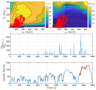
Figure 6: Base H₂-vehicle operating conditions on the WLTC. Top: Engine operating points superimposed on the engine efficiency map and the NO${}_{\mathrm{x}}^{\mathrm{eo}}$ map. Middle: Time-resolved and normalized NO${}_{\mathrm{x,0}}^{\mathrm{eo}}$ emissions. Bottom: Velocity profile of the WLTC with NO${}_{\mathrm{x,0}}^{\mathrm{eo}}$ peaks marked by red dots.

3.2 Hybridized drivetrains

As the base H₂-vehicle cannot reliably ensure extremely low NO${}_{\mathrm{x,0}}^{\mathrm{eo}}$ emissions, an investigation is conducted below about how the mixed H₂-HEV is able to reach lower NO${}_{\mathrm{x}}^{\mathrm{eo}}$ emissions. Comparing the red and the yellow lines in Figure 5 shows that the H₂ saving potential of the series H₂-HEV and the parallel H₂-HEV are comparable on the WLTC. The EMS calibrations, which are indicated by the intersections of the Pareto fronts with the black, dotted line reveal that the series H₂-HEV is able to obtain a 0.8% lower H₂ consumption compared to the parallel H₂-HEV. With the mixed H₂-HEV architecture however, the H₂ saving potential is 5%, compared to the parallel H₂-HEV. To understand how the mixed H₂-HEV’s EMS is able to reduce the accumulated NO${}_{\mathrm{x}}^{\mathrm{eo}}$ emissions, the solutions $\mathcal{S}^{\star}$ and $\mathcal{S}^{--}$ of this drivetrain architecture are compared below.

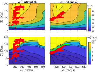
Figure 7: Left: Engine operating points superimposed on the engine efficiency map and the NO${}_{\mathrm{x}}^{\mathrm{eo}}$ map resulting of the EMS calibration $\mathcal{S}^{\star}$. Right: Engine operating points superimposed on the engine efficiency map and the NO${}_{\mathrm{x}}^{\mathrm{eo}}$ map resulting of the EMS calibration $\mathcal{S}^{--}$.

Figure 7 depicts the engine operating points of these two solutions, superimposed on the engine efficiency map and the NO${}_{\mathrm{x}}^{\mathrm{eo}}$ map. Two things can be noticed here: Firstly, it is optimal in both scenarios to omit low-load engine operating points, i.e., $T_{e}\lessapprox 45$ Nm. This is a well-known result and usually one of the main drivers to reduce the overall fuel consumption of any HEV equipped with a combustion engine. Secondly, the optimal EMS calibration $\mathcal{S}^{--}$ is achieved by omitting too high-load engine operating points. The maximum engine torque does not surpass the NO${}_{\mathrm{x}}^{\mathrm{eo}}$-isoline, which is highlighted by the green line. Above this line, the emitted NO${}_{\mathrm{x}}^{\mathrm{eo}}$ increase rapidly, as ultra-lean operation of the H₂ICE is no longer possible.

4 Different Driving Missions

So far, it was shown that the mixed H₂-HEV has superior performance compared to the other H₂-HEVs and the base H₂-vehicle. In the following, to further highlight the potential for reducing the NO${}_{\mathrm{x}}^{\mathrm{eo}}$ of this drivetrain structure, a specific EMS calibration is selected, which achieves 90% less NO${}_{\mathrm{x}}^{\mathrm{eo}}$ than the base H₂ vehicle. It is denoted by $\mathcal{S}^{\blacktriangle}$.

The remainder of this publication is used to investigate whether the potential of the mixed H₂-HEV to reduce the NO${}_{\mathrm{x}}^{\mathrm{eo}}$ emissions can be generalized to other driving missions. Consequently, four additional driving missions are introduced and their corresponding Pareto fronts are presented. The first two represent more realistic driving scenarios. The third and the fourth driving mission are used to show the limitations of the mixed H₂-HEV powertrain architecture to reduce NO${}_{\mathrm{x}}^{\mathrm{eo}}$.

Finally, most state-of-the-art EMS algorithms (e.g., [26], [27]) only pay attention to minimizing the H₂ consumption resulting (in the best case) in $\mathcal{S}^{\star}$. As in this work, the possibility to decrease the NO${}_{\mathrm{x}}^{\mathrm{eo}}$ at the expense of an increased H₂ consumption is discussed, three additional key parameters are introduced below. On the one hand, they serve the purpose of facilitating a contrast between different realizations of the H₂-NO${}_{\mathrm{x}}^{\mathrm{eo}}$ trade-off, and on the other hand, they emphasize the advantages of the hybridization of the base H₂-vehicle. In particular, the EMS calibration $\mathcal{S}^{\blacktriangle}$ is investigated, as it provides a substantial decrease in NO${}_{\mathrm{x}}^{\mathrm{eo}}$ at a marginally increased H₂ consumption. For convenience, and to enable a comparison among the individual driving missions, all key parameters are summarized in Table 4.

Key performance parameters:
Firstly, if not the H₂-optimal EMS calibration is chosen, but instead the EMS calibration $\mathcal{S}^{\blacktriangle}$, the following increase in H₂ consumption occurs:

$$\Delta\mathrm{H}_{2}^{\mathrm{add}}=1-\frac{\mathrm{H}_{2}^{\mathcal{S}^{\star}}}{\mathrm{H}_{2}^{\mathcal{S}^{\blacktriangle}}}.$$ (27)

Secondly, the highest possible NO${}_{\mathrm{x}}^{\mathrm{eo}}$ emissions reduction of the mixed H₂-HEV compared to the base H₂-vehicle calculates as:

$$f_{\mathrm{x}}^{\mathrm{eo,}\mathcal{S}^{\blacksquare}}=\frac{\mathrm{NO}_{\mathrm{x}}^{\mathrm{eo,}\mathcal{S}^{\blacksquare}}}{\mathrm{NO}_{\mathrm{x,0}}^{\mathrm{eo}}}.$$ (28)

It is achieved by the EMS calibration $\mathcal{S}^{\blacksquare}$ and it describes the mixed H₂-HEV’s limit to reduce NO${}_{\mathrm{x}}^{\mathrm{eo}}$.

Thirdly, the last key parameter describes how much H₂ the mixed H₂-HEV saves, while aiming for a reduction of 90% NO${}_{\mathrm{x}}^{\mathrm{eo}}$ emissions, compared to the base H₂-vehicle:

$$\Delta\mathrm{H}_{2}=1-\frac{\mathrm{H}_{2}^{\mathcal{S}^{\blacktriangle}}}{\mathrm{H}_{2,0}}.$$ (29)

It is mainly used to showcase how powerful the hybridization of a vehicle with an H₂ICE can be.

4.1 Realistic Driving Scenarios

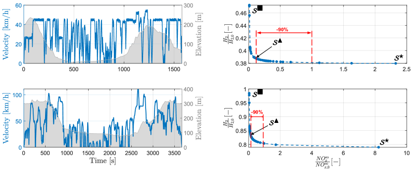
Figure 8: Left: Driving missions: ”urban cycle” and ”real driving cycle”. Right: H₂-NO${}_{\mathrm{x}}^{\mathrm{eo}}$ Pareto-optimal operations of the mixed H₂-HEV for the corresponding driving missions. The results are normalized using H_2,0 and NO${}_{x,0}^{\mathrm{eo}}$ of the base H₂-vehicle. Three EMS calibrations, i.e., $\mathcal{S}^{\star}$, $\mathcal{S}^{\blacktriangle}$, and $\mathcal{S}^{\blacksquare}$ are highlighted for the mixed H₂-HEV and both driving cycles.

On the left hand side of Figure 8, two additional realistic driving scenarios are depicted. The first driving mission is extracted from the open-source software SUMO [32] and is referred to as urban cycle. The second driving mission is based on recorded sensor data of a real vehicle and features a mix of urban driving, rural driving, and highway driving. It is referred to as real driving cycle. Both missions feature an extensive elevation profile.

On the right hand side of Figure 8, the corresponding H₂-NO${}_{\mathrm{x}}^{\mathrm{eo}}$ Pareto fronts are depicted for both driving missions. For both driving missions, there exist EMS calibrations $\mathcal{S}^{\blacktriangle}$ achieving the intended significant NO${}_{\mathrm{x}}^{\mathrm{eo}}$ reductions. The factor $\Delta\mathrm{H}_{2}^{\mathrm{add}}$ shows that these large reductions in NO${}_{\mathrm{x}}^{\mathrm{eo}}$ come at an increased hydrogen consumption of only 2.2% (urban cycle), or 5.8% (real driving cycle). The factor $\Delta\mathrm{H}_{2}$ shows that it is possible to reduce the base H₂-vehicle’s NO${}_{\mathrm{x}}^{\mathrm{eo}}$ emissions by 90%, while still saving 61.2% (urban cycle), or 16.1% (real driving cycle), respectively. Finally, an even lower NO${}_{\mathrm{x}}^{\mathrm{eo}}$ emission level can be achieved, i.e., $f_{\mathrm{x}}^{\mathrm{eo,}\mathcal{S}^{\blacksquare}}=$ 99% and $f_{\mathrm{x}}^{\mathrm{eo,}\mathcal{S}^{\blacksquare}}=$ 96.6% on the urban cycle, and the real driving cycle, respectively.

4.2 Worst-case driving scenarios

The analysis of the Pareto fronts obtained for the urban cycle and the real driving cycle show that for driving patterns that are likely to occur during day-to-day driving, the mixed H₂-HEV provides a large range of H$2$-NO${}_{\mathrm{x}}^{\mathrm{eo}}$ trade-offs to choose from. This section now focuses on extreme driving scenarios, which are chosen to show the limitations of the mixed H₂-HEV. The main tool to decrease the NO${}_{\mathrm{x}}^{\mathrm{eo}}$ emissions via hybridization of the propulsion architecture bases on omitting too high engine-load operating points. So far, the investigated driving missions all include a broad range of different torque requests, and, for these missions, the results obtained by DP show that the mixed H₂-HEV is a promising topology to enable a large range of realizable H₂-NO${}_{\mathrm{x}}^{\mathrm{eo}}$ trade-offs. Therefore, two additional driving missions are presented in the following, which mainly consist of high torque requests.

Mountain Cycle:
The left hand side of Figure 9 depicts the mountain cycle, which is inspired by a mountain pass in the Swiss alps, and represents a trip including a continuous climb of over 1270 m. It is assumed that no other road users are present, i.e., other than in the hairpin turns, the vehicle speed is constant at 70 km/h.

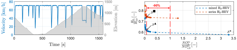
Figure 9: Left: Driving missions: ”mountain cycle”. Right: H₂-NO${}_{\mathrm{x}}^{\mathrm{eo}}$ Pareto-optimal operations of the mixed H₂-HEV for the ”mountain cycle”. The results are normalized using H_2,0 and NO${}_{x,0}^{\mathrm{eo}}$ of the base H₂-vehicle. Three EMS calibrations, i.e., $\mathcal{S}^{\star}$, $\mathcal{S}^{\blacktriangle}$, and $\mathcal{S}^{\blacksquare}$ are highlighted for the mixed H₂-HEV.

The right hand side of Figure 9 depicts in blue the achievable Pareto-optimal H₂-NO${}_{\mathrm{x}}^{\mathrm{eo}}$ trade-off for the mixed H₂-HEV on the mountain cycle. To highlight the importance of the parallel mode for this kind of driving missions below, the series H₂-HEV’s Pareto front is shown in red. There exists an EMS calibration $\mathcal{S}^{\blacktriangle}$, which achieves the intended significant NO${}_{\mathrm{x}}^{\mathrm{eo}}$ reductions. It results in an increase of hydrogen consumption of $\Delta H_{2}^{\mathrm{add}}=5.9\%$. The factor $\Delta\mathrm{H}_{2}$ shows that it is possible to reduce the base H₂-vehicle’s emissions by 90%, while saving 38.9% H₂. Finally, an even lower NO${}_{\mathrm{x}}^{\mathrm{eo}}$ emission level can be achieved, i.e., $f_{\mathrm{x}}^{\mathrm{eo,}\mathcal{S}^{\blacksquare}}=$ 98.6%, showing that despite the considerable power demand required for ascending the elevation, the mixed H₂-HEV is able to decrease the NO${}_{\mathrm{x}}^{\mathrm{eo}}$ emissions with a proper EMS calibration.

Comparing the blue and red Pareto fronts shows that the mixed H₂-HEV is able to utilize the parallel mode to effectively decrease the H₂ consumption. How the parallel mode is used, is outlined in the following: Figure 10 displays the optimal distribution of the torque request between the engine and the motor, evaluated at the differential. The torque distribution is only shown for the parallel mode of the two Pareto-optimal EMS calibrations $\mathcal{S}^{\blacktriangle}$ and $\mathcal{S}^{\star}$. First of all, the optimal engine usage (depicted by the circles) is analyzed for both EMS calibrations: For torque requests below 100 Nm it is optimal to use load-point shifting (,i.e., increasing the produced engine power above what is required at the wheel to store excess power via the motor in the battery) to additionally recharge the battery. This is depicted by $T_{e}$ above the dashed 45^∘-line. This allows to simultaneously operate the H₂ICE in a higher efficiency operating point (without getting into the high-NO${}_{\mathrm{x}}^{\mathrm{eo}}$ region) and to further charge the battery with electric energy that can be spent later on. The total positive electric energy throughput in EV mode is decreased by roughly 65% (from 4.1 MJ in $\mathcal{S}^{\star}$ to 2.6 MJ in $\mathcal{S}^{\blacktriangle}$). This shows that, over the entire driving mission, the usage of EV mode is decreased, and the battery electric energy is increasingly used in parallel mode. While driving in parallel mode, the electric energy is used to relieve the engine of too high load-points that occur during uphill driving. Focusing on the blue circles, the H₂-optimal EMS calibration is obtained by respecting a (slightly scattered,) preferred maximum engine torque, which is achieved by additionally boosting with the electric motor (indicated by the red crosses). The electric motor is used such that the H₂ICE is run in its highest speed-dependent fuel-efficiency operating points (compare to Figure 3).

The yellow circles and purple crosses represent the engine torque and the motor torque for the EMS calibration $\mathcal{S}^{\blacktriangle}$. Again, there exists an upper engine torque limit at around 100 Nm, until which the entire torque request is supplied solely by the engine, and beyond which any additional torque request is supplied by boosting with the motor. However, here this bound is more distinct and lower than in $\mathcal{S}^{\star}$, revealing that the electric motor is used to prevent high engine torques.

Comparing the blue and red Pareto fronts in Figure 9, the importance of the parallel mode for this driving missions is demonstrated. Although, extremely low NO${}_{\mathrm{x}}^{\mathrm{eo}}$ emissions can be achieved by the series H₂-HEV, these EMS calibrations can come at a relatively high H₂ consumption, when compared to the mixed H₂-HEV. In conclusion, electric boosting in parallel mode is utilized by the mixed H₂-HEV to operate the H₂ICE under extremely low NO${}_{\mathrm{x}}^{\mathrm{eo}}$ conditions, while still keeping the H₂ consumption at a low level. However, this torque distribution strategy is only viable, if the driving missions offers enough potential for circulating energy, i.e., energy that is stored temporarily in the vehicle body as kinetic and potential energy and used to recharge the battery.

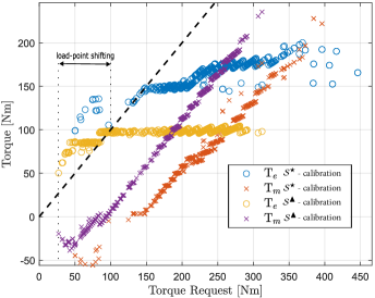
Figure 10: Distribution of the torque request of two optimal EMS calibrations (i.e., $\mathcal{S}^{\blacktriangle}$, $\mathcal{S}^{\blacksquare}$) of the mixed H₂-HEV on the mountain cycle. Only the parallel mode is displayed. The black dashed line represents the 45^∘-line.

Highway Cycle:

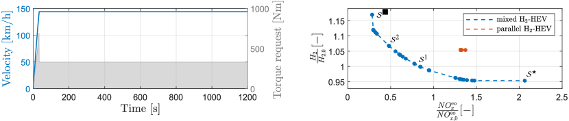
Figure 11: Left: Driving missions: ”highway cycle”. Right: H₂-NO${}_{\mathrm{x}}^{\mathrm{eo}}$ Pareto-optimal operations of the mixed H₂-HEV for the ”highway cycle”. The results are normalized using H_2,0 and NO${}_{x,0}^{\mathrm{eo}}$ of the base H₂-vehicle. Four EMS calibrations, i.e., $\mathcal{S}^{\star}$, $\mathcal{S}^{1}$, $\mathcal{S}^{2}$, and $\mathcal{S}^{\blacksquare}$ are highlighted for the mixed H₂-HEV.

As was shown for the mountain cycle, circulating energy is leveraged by the mixed H₂-HEV to achieve a broad range of H₂-NO${}_{\mathrm{x}}^{\mathrm{eo}}$ trade-offs. The following cycle is constructed such that it offers no circulating energy at all. The left hand side of Figure 11 depicts the highway cycle. Similar to the mountain cycle, high torque requests occur in this scenario. The difference is that the highway cycle is an artificial scenario, which is constructed to solely consist of high, positive torque requests: After a short acceleration phase, the vehicle reaches a constant speed of 142 km/h, which requires a torque request of 372 Nm at the wheel to maintain the speed level for the rest of the driving mission. In parallel mode, this requirement translates to an engine speed of $\omega_{e}$ = 352 rad/s. If the engine was to provide the full torque request on its own, it would need to provide a torque of $T_{e}=$ 153 Nm, which results in a good fuel efficiency, but cannot be sustained under ultra-lean combustion conditions and therefore results in high NO${}_{\mathrm{x}}^{\mathrm{eo}}$ emissions. Decreasing the engine load via electric boosting and thereby lowering the NO${}_{\mathrm{x}}^{\mathrm{eo}}$ is infeasible: On the one hand, the EMS is required to satisfy the charge-sustainability constraint (26f) over the entire driving mission. On the other hand, this driving mission offers no opportunities to recuperate braking energy or to use load point shifting, as the goal is to reduce the engine load.
The right hand side of Figure 11 depicts the achievable Pareto-optimal H₂-NO${}_{\mathrm{x}}^{\mathrm{eo}}$ trade-offs for the the parallel H₂-HEV and the mixed H₂-HEV in red and blue, respectively. Most notably is that the EMS calibration $\mathcal{S}^{\blacktriangle}$ cannot be reached, given that the reduction of NO${}_{\mathrm{x}}^{\mathrm{eo}}$ emissions to that extent is unattainable. The lowest possible cumulated NO${}_{\mathrm{x}}^{\mathrm{eo}}$ emissions are $f_{\mathrm{x}}^{\mathrm{eo,}\mathcal{S}^{\blacksquare}}$ = 71.6% lower than what is achieved by the base H₂-vehicle. But, this reduction of NO${}_{\mathrm{x}}^{\mathrm{eo}}$ comes at the cost of a greatly increased H₂ consumption, which is 17% higher than the base H₂-vehicle, and 18.5% higher than the H₂-optimal EMS calibration $\mathcal{S}^{\star}$. This significant rise in H₂ consumption is primarily due to the fact that the base H₂-vehicle can almost exclusively operate its H₂ICE at a highly efficient operating point, meaning that a hybridized drivetrain can not increase its mean efficiency by any significant amount. However, the mixed H₂-HEV is still able to offer great flexibility to adjust the H₂-NO${}_{\mathrm{x}}^{\mathrm{eo}}$ trade-off, which heavily depends on the usage of the series mode.

Figure 12 provides further insight into how four different optimal EMS calibrations, i.e., $\mathcal{S}^{\star}$, $\mathcal{S}^{1}$, $\mathcal{S}^{2}$, and $\mathcal{S}^{\blacksquare}$, use the series mode to achieve the corresponding values for the cumulated NO${}_{\mathrm{x}}^{\mathrm{eo}}$ emissions. For each EMS calibration, the complete set of engine operating points is shown in the NO${}_{\mathrm{x}}^{\mathrm{eo}}$-emissions map. Following the graphs from the top left towards the bottom right, the individual strategies depicted reduce the cumulated NO${}_{\mathrm{x}}^{\mathrm{eo}}$ step by step. Green circles indicate parallel mode with additional support of the electric motor, blue circles indicate parallel mode where only the H₂ICE produces power (comparable to a conventional vehicle), and red circles indicate series mode. The size of the circles indicates the amount of times that the corresponding operating point is chosen. For the H₂-optimal EMS calibration $\mathcal{S}^{\star}$, most of the cycle is driven solely using the H₂ICE. The parallel mode is used at the beginning to assist in the acceleration of the vehicle with the electric motor, before the H₂ICE takes over shortly before reaching 142 km/h.
When gradually decreasing the cumulated NO${}_{\mathrm{x}}^{\mathrm{eo}}$, three changes in the optimal EMS calibration can be identified. Firstly, pure conventional driving is substituted by an electrically assisted use of the H₂ICE, which is indicated by replacing the blue circle with a green one. The electric energy needed to ensure charge-sustainability is generated via the series mode. Secondly, when transitioning from $\mathcal{S}^{1}$ to $\mathcal{S}^{2}$, a shift from parallel mode to series mode is observed, which is indicated by the growing size of the red circles and a shrinking size of the green circle. This ultimately leads to solely operating the vehicle in series mode. Thirdly, in series mode, the H₂ICE operating points are shifted to ever higher engine speeds the lower the cumulated NO${}_{\mathrm{x}}^{\mathrm{eo}}$ emissions get. The reason for this transition is given by the fact that it allows to sustain the engine power output, while decreasing the engine torque. This enables the engine-generator unit to deliver electric power to the motor or the battery, without increasing (or even decreasing) the NO${}_{\mathrm{x}}^{\mathrm{eo}}$ emissions. However, this shift comes at the price of an increased H₂ consumption, as the engine efficiency drops above approximately 230 rad/s. In conclusion, the series mode is utilized by the mixed H₂-HEV to achieve extremely low cumulated NO${}_{\mathrm{x}}^{\mathrm{eo}}$ emissions, even if not enough circulated energy can be recuperated. However, there is a limit to the maximum torque request that can be provided under ultra-lean combustion conditions. At some point, the torque request is too large and the engine-generator unit cannot shift to ever higher engine speeds. As a result, $T_{e}$ has to be increased, which directly leads to increased NO${}_{\mathrm{x}}^{\mathrm{eo}}$ emissions.

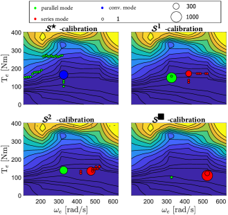
Figure 12: Engine operating points on the highway cycle. The size of the dots represents how often that the corresponding operating point has been chosen.

Table 4: Summary of key performance indicators of the mixed H₂-HEV for various investigated driving missions. As $\mathcal{S}^{\blacktriangle}$ cannot be realized on the highway cycle, the metrics ”$\Delta H_{2}^{\mathrm{add}}$” and ”$\Delta H_{2}$” are calculated with respect to $\mathcal{S}^{\blacksquare}$, which is denoted with the superscript ”^■” in the corresponding columns.

	$\Delta\mathrm{H}_{2}^{\mathrm{add}}$	$\Delta\mathrm{H}_{2}$	$f_{\mathrm{x}}^{\mathrm{eo,\mathcal{S}^{\blacksquare}}}$
Urban cycle	2.2%	61.2%	99%
Real driving cycle	5.8%	16.1%	96.6%
Mountain cycle	5.9%	38.9%	98.6%
Highway cycle	18.5%■	-17%■	71.6%

5 Conclusion

To the authors’ best knowledge, this paper provides the first full potential analysis of electrically hybridized vehicles equipped with an H₂ICE. A wide flexibility for choosing a Pareto-optimal trade-off between H₂ consumption and NO${}_{\mathrm{x}}^{\mathrm{eo}}$ emissions can be achieved, solely by changing the distribution of the torque request between the vehicle’s power sources. Overall, the performance of three different hybridized powertrain solutions, i.e., a series H₂-HEV, a parallel H₂-HEV, and a mixed H₂-HEV, are compared to a base H₂-vehicle on the WLTC. The resulting Pareto-optimal H₂-NO${}_{\mathrm{x}}^{\mathrm{eo}}$ trade-offs show two things: Firstly, all investigated H₂-HEVs greatly outperform the base H₂-vehicle. Secondly, the mixed H₂-HEV is the superior H₂-HEV architecture in both regards: H₂ consumption and NO${}_{\mathrm{x}}^{\mathrm{eo}}$ emissions.

To solidify the findings obtained on the WLTC, the performance potential of the mixed H₂-HEV is further investigated on a variety of different realistic driving missions. The mixed H₂-HEV effectively leverages both the parallel mode and the series mode to lower the H₂ consumption and reach extremely low NO${}_{\mathrm{x}}^{\mathrm{eo}}$ emissions, respectively: To reduce the H₂ consumption by increasing the drivetrain’s overall efficiency, the parallel mode is used. To achieve extremely low NO${}_{\mathrm{x}}^{\mathrm{eo}}$ emissions by decoupling the H₂ICE, which allows to run it in its most suitable operating point, the series mode is used. For a broad range of driving missions, the mixed H₂-HEV is able to decrease the engine-out NO${}_{\mathrm{x}}^{\mathrm{eo}}$ emissions by 90%, while, at the same time, decreasing the H₂ consumption by over 16%, compared to the base H₂-vehicle. These significant emission reductions are possible without having to modify the exhaust-gas aftertreatment system, or the optimization of any of the individual drivetrain components, but solely by setting the EMS calibration accordingly.

Further research could focus on the development of an online-capable control algorithm for the energy management of the investigated mixed H₂-HEV. The goal would be to reach close-to-optimal H₂ consumption, while satisfying a NO${}_{\mathrm{x}}^{\mathrm{eo}}$ emission target. The technique of model predictive control could be used to calculate the optimal torque split in real-time. Another direction of research could be the development and inclusion of an additional dynamic NO${}_{\mathrm{x}}^{\mathrm{eo}}$ emissions model and the analysis of its influence on the H₂-NO${}_{\mathrm{x}}^{\mathrm{eo}}$ Pareto front of the mixed H₂-HEV. Also, the reduced NO${}_{\mathrm{x}}^{\mathrm{eo}}$ emissions lead to changed requirements for the exhaust-gas aftertreatment system, creating an avenue for exploring the optimization of EMS calibration in conjunction with the design and operation of the exhaust gas aftertreatment system.

References

- Parra et al. [2019] D. Parra, L. Valverde, F. J. Pino, M. K. Patel, A review on the role, cost and value of hydrogen energy systems for deep decarbonisation, Renewable and Sustainable Energy Reviews 101 (2019) 279–294.
- Abe et al. [2019] J. O. Abe, A. Popoola, E. Ajenifuja, O. M. Popoola, Hydrogen energy, economy and storage: Review and recommendation, International journal of hydrogen energy 44 (2019) 15072–15086.
- Colbertaldo et al. [2019] P. Colbertaldo, S. B. Agustin, S. Campanari, J. Brouwer, Impact of hydrogen energy storage on California electric power system: Towards 100% renewable electricity, International Journal of Hydrogen Energy 44 (2019) 9558–9576.
- [4] I. E. A. (IEA), CO2 emissions in 2022, International Energy Agency (2022).
- EPA [2021] EPA, epa.gov, https://www.epa.gov/regulations-emissions-vehicles-and-engines/final-rule-revise-existing-national-ghg-emissions (2021). Accessed on June 08, 2023.
- EU Regulation [2019] EU Regulation, Regulation (EU) 2019/631 of the European parliament and of the council of 17 April 2019 setting CO2 emission performance standards for new passenger cars and for new light commercial vehicles, and repealing Regulations (EC) no 443/2009 and (eu) no 510/2011, URL https://eur-lex. europa. eu/legalcontent/EN/TXT (2019).
- Gersdorf et al. [2020] T. Gersdorf, P. Hertzke, P. Schaufuss, S. Schenk, McKinsey electric vehicle index: Europe cushions a global plunge in EV sales, 2020.
- Du et al. [2021] Z. Du, C. Liu, J. Zhai, X. Guo, Y. Xiong, W. Su, G. He, A review of hydrogen purification technologies for fuel cell vehicles, Catalysts 11 (2021) 393.
- Shinde and Karunamurthy [2022] B. J. Shinde, K. Karunamurthy, Recent progress in hydrogen fuelled internal combustion engine (H2ICE)–a comprehensive outlook, Materials Today: Proceedings 51 (2022) 1568–1579.
- Falfari et al. [2023] S. Falfari, G. Cazzoli, V. Mariani, G. M. Bianchi, Hydrogen application as a fuel in internal combustion engines, Energies 16 (2023) 2545.
- Onorati et al. [2022] A. Onorati, R. Payri, B. Vaglieco, A. Agarwal, C. Bae, G. Bruneaux, M. Canakci, M. Gavaises, M. Günthner, C. Hasse, et al., The role of hydrogen for future internal combustion engines, 2022.
- Stkepień [2021] Z. Stkepień, A comprehensive overview of hydrogen-fueled internal combustion engines: achievements and future challenges, Energies 14 (2021) 6504.
- Rouleau et al. [2021] L. Rouleau, F. Duffour, B. Walter, R. Kumar, L. Nowak, Experimental and numerical investigation on hydrogen internal combustion engine, Technical Report, SAE Technical Paper, 2021.
- EU Regulation [2022] EU Regulation, Proposal for a regulation of the european parliament and of the council on type-approval of motor vehicles and engines and of systems, components and separate technical units intended for such vehicles, with respect to their emissions and battery durability (Euro 7) and repealing Regulations (EC) No 715/2007 and (EC) No 595/2009, URL https://ec.europa.eu/transparency/documents-register/detail?ref=COM(2022)586&lang=en (2022).
- White et al. [2006] C. White, R. Steeper, A. Lutz, The hydrogen-fueled internal combustion engine: a technical review, International journal of hydrogen energy (2006).
- Heffel [2003a] J. W. Heffel, NOx emission reduction in a hydrogen fueled internal combustion engine at 3000 rpm using exhaust gas recirculation, International Journal of Hydrogen Energy 28 (2003a) 1285–1292.
- Heffel [2003b] J. W. Heffel, NOx emission and performance data for a hydrogen fueled internal combustion engine at 1500rpm using exhaust gas recirculation, International Journal of Hydrogen Energy 28 (2003b) 901–908.
- Bao et al. [2022] L.-z. Bao, B.-g. Sun, Q.-h. Luo, Experimental investigation of the achieving methods and the working characteristics of a near-zero NOx emission turbocharged direct-injection hydrogen engine, Fuel 319 (2022) 123746.
- Sementa et al. [2022] P. Sementa, J. B. de Vargas Antolini, C. Tornatore, F. Catapano, B. M. Vaglieco, J. J. L. Sánchez, Exploring the potentials of lean-burn hydrogen SI engine compared to methane operation, International Journal of Hydrogen Energy 47 (2022) 25044–25056.
- Sciarretta et al. [2014] A. Sciarretta, L. Serrao, P. Dewangan, P. Tona, E. Bergshoeff, C. Bordons, L. Charmpa, P. Elbert, L. Eriksson, T. Hofman, et al., A control benchmark on the energy management of a plug-in hybrid electric vehicle, Control engineering practice 29 (2014) 287–298.
- Ritzmann et al. [2019] J. Ritzmann, A. Christon, M. Salazar, C. Onder, Fuel-optimal power split and gear selection strategies for a hybrid electric vehicle, Technical Report, SAE Technical Paper, 2019.
- Serrao et al. [2011] L. Serrao, S. Onori, A. Sciarretta, Y. Guezennec, G. Rizzoni, Optimal energy management of hybrid electric vehicles including battery aging, in: Proceedings of the 2011 American control conference, IEEE, 2011, pp. 2125–2130.
- Ritzmann et al. [2021] J. Ritzmann, O. Chinellato, R. Hutter, C. Onder, Optimal integrated emission management through variable engine calibration, Energies 14 (2021) 7606.
- He et al. [2006] X. He, T. Maxwell, M. E. Parten, Development of a hybrid electric vehicle with a hydrogen-fueled IC engine, IEEE transactions on vehicular technology 55 (2006) 1693–1703.
- Jaura et al. [2004] A. K. Jaura, W. Ortmann, R. Stuntz, B. Natkin, T. Grabowski, Ford’s H2RV: An Industry First HEV Propelled with a H2 Fueled Engine-A Fuel Efficient and Clean Solution for Sustainable Mobility, Technical Report, SAE Technical Paper, 2004.
- Beccari [2022] S. Beccari, On the use of a hydrogen-fueled engine in a hybrid electric vehicle, Applied Sciences 12 (2022) 12749.
- Kyjovskỳ et al. [2023] Š. Kyjovskỳ, J. Vávra, I. Bortel, R. Toman, Drive cycle simulation of light duty mild hybrid vehicles powered by hydrogen engine, International Journal of Hydrogen Energy 48 (2023) 16885–16896.
- Guzzella et al. [2013] L. Guzzella, A. Sciarretta, et al., Vehicle propulsion systems, volume 3, Springer, 2013.
- Widmer et al. [2022] F. Widmer, A. Ritter, P. Duhr, C. H. Onder, Battery lifetime extension through optimal design and control of traction and heating systems in hybrid drivetrains, ETransportation 14 (2022) 100196.
- Powell [2007] W. B. Powell, Approximate Dynamic Programming: Solving the curses of dimensionality, volume 703, John Wiley & Sons, 2007.
- Uebel et al. [2017] S. Uebel, N. Murgovski, C. Tempelhahn, B. Bäker, Optimal energy management and velocity control of hybrid electric vehicles, IEEE Transactions on Vehicular Technology 67 (2017) 327–337.
- Behrisch et al. [2011] M. Behrisch, L. Bieker, J. Erdmann, D. Krajzewicz, Sumo–simulation of urban mobility: an overview, in: Proceedings of SIMUL 2011, The Third International Conference on Advances in System Simulation, ThinkMind, 2011.