DFL-TORO: A One-Shot Demonstration Framework for Learning Time-Optimal Robotic Manufacturing Tasks

Abstract

This paper presents DFL-TORO, a novel Demonstration Framework for Learning Time-Optimal Robotic tasks via One-shot kinesthetic demonstration. It aims at optimizing the process of Learning from Demonstration (LfD), applied in the manufacturing sector. As the effectiveness of LfD is challenged by the quality and efficiency of human demonstrations, our approach offers a streamlined method to intuitively capture task requirements from human teachers, by reducing the need for multiple demonstrations. Furthermore, we propose an optimization-based smoothing algorithm that ensures time-optimal and jerk-regulated demonstration trajectories, while also adhering to the robot’s kinematic constraints. The result is a significant reduction in noise, thereby boosting the robot’s operation efficiency. Evaluations using a Franka Emika Research 3 (FR3) robot for a reaching task further substantiate the efficacy of our framework, highlighting its potential to transform kinesthetic demonstrations in contemporary manufacturing environments.

I Introduction

In the manufacturing industry, the transition from mass production to mass customization [1] necessitates flexible robot programming adaptable to frequently changing tasks[2]. Traditional programming, with its reliance on robot experts, increases costs and downtime [3]. As a solution, Learning from Demonstration (LfD) [4] allows robots to learn tasks flexibly from non-experts [5]. However, deploying LfD in practical manufacturing settings poses performance challenges [6, 4], which motivates the current work.

In robotic manufacturing, the performance can be evaluated based on “Implementation Efficiency” and “Operation Efficiency” metrics [4]. Implementation efficiency pertains to the resources required for teaching a task, while operation efficiency considers production speed against ongoing costs such as maintenance and robot wear and tear. Often, the quality and the procedure of acquiring demonstrations are sub-optimal with respect to the mentioned metrics [7]. Our focus in this paper is to address the challenges faced when attempting to acquire information-rich demonstrations in an efficient manner, in order to enable LfD algorithms to optimally learn and generalize tasks.

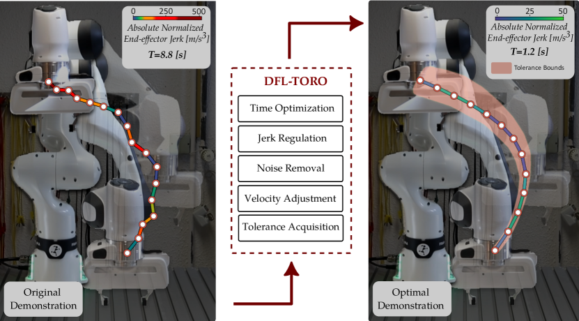
Figure 1: Advantages of DFL-TORO

Human demonstrations inherently dictate the requirements of a “correct” execution of a task. While LfD’s aim is not to mirror the demonstration but to grasp the core recipe, it is vital to assign significance to each segment of the demonstration. This highlights how much variation the robot can tolerate while still fulfilling the task reliably. For instance, in a Reaching task, high precision is required while approaching a target, but the initial motion can vary without undermining reliability. This variation can be encoded as a set of tolerance values, capturing the task’s pivotal points and providing flexibility. However, providing such detailed demonstrations is challenging. Existing methods rely on multiple demonstration statistics to deduce these tolerances, which reduces implementation efficiency.

Humans demonstrate tasks slowly due to the cognitive complexity of illustrating various aspects simultaneously [8]. As minimizing the execution time is a crucial factor, it is essential to obtain the most optimal timing law. Most existing LfD methods address this by letting humans speed up initial demonstrations [9]. However, the robot’s kinematic limits are often overlooked, with no guarantee of achieving the optimal time in practice. Complicating this, human demonstrations can be noisy from hand trembling or sensor errors, resulting in jerky trajectories. Speeding up such demonstrations can amplify the irregularities, causing erratic motions, raising maintenance costs, and wasting energy. Moreover, LfD algorithms are likely to overfit and mimic this noise. These issues collectively diminish operation efficiency, underscoring the importance of smooth and time-optimal demonstrations.

Given the outlined challenges, this paper introduces DFL-TORO, a novel Demonstration Framework for Learning Time-Optimal Robotic tasks via One-shot kinesthetic demonstration. DFL-TORO intuitively captures human demonstrations and obtains task tolerances, yielding smooth, jerk-regulated, timely, and noise-free trajectories, as illustrated in Fig. 1. Our main contributions are as follows:

• An optimization-based smoothing algorithm, considering the robot’s kinematic limits and task tolerances, which delivers time-and-jerk optimal trajectories and filters out the noise, enhancing operation efficiency.

• A method for intuitive refinement of velocities and acquisition of tolerances, reducing the need for repetitive demonstrations and boosting operational efficiency.

• Evaluation of DFL-TORO for a Reaching task via Franka Emika Research 3 (FR3) robot, highlighting its superiority over conventional kinesthetic demonstrations, using Dynamic Movement Primitives (DMPs) [10].

II Background and Related Work

Recent literature has shifted from focusing on robustness against sub-optimal demonstrations [11] towards assessing the information gain and quality of demonstrations [7, 12]. To do so, several studies have employed incremental learning to simplify the demonstration process, enabling humans to teach task components in phases. Authors in [13] let humans demonstrate path and timing separately, by allowing them to adjust the speed of their initial demonstration. The proposed framework in [9] enables path and speed refinement through kinesthetic guidance, while the one in [8] uses teleoperated feedback for efficient task execution. Building on these, our approach incorporates the robot’s kinematic limits into an optimization problem, solving for the best feasible timing law for the demonstrated path. Then, instead of merely speeding up, we permit users to “slow down” demonstrations until reliable execution, and hence ensure the optimal timing.

Task variability tolerances are primarily used to adjust a robot’s impedance, e.g., low impedance when there is high variability [14], but they are also pivotal for noise removal. Given that demonstrations do not have a set ground truth, distinguishing signals from noise is challenging. Using tolerances as trajectory guidelines ensures the trajectory is with the desired accuracy, preserving the demonstration’s authenticity [15]. The study in [16] offers a detailed comparison of various smoothing algorithms, and the noise-removing effect of RBF-based methods like DMPs. However, without careful hyperparameter tuning, they risk overfitting and noise replication. The study concludes that optimization-based smoothing is more effective in preserving demonstration features and improving information gain. Within this context, some works have omitted tolerances [17] or used fixed user-defined tolerances [18]. However, our approach extracts these tolerances directly from human demonstrations and incorporates them into the optimization.

To deduce tolerances from human demonstrations, it is common to consider the variance of multiple demonstrations, as an indicator of variability tolerance [19, 20, 15]. To enhance implementation efficiency, we propose a novel approach to discern tolerances from a single demonstration. Grounded in the psychological observation that humans naturally slow down when aiming for precision [21], our method captures tolerances during periods where the demonstrator slows down. Although demonstrations are presented in joint space, we extract tolerances in the Cartesian space, emphasizing the end-effector pose as the task’s crucial point.

It has remained a challenge to simultaneously optimize for time and jerk, as might create an infeasible problem. This stems from the fact that applying path constraints requires knowing the relative time when each part of the path is reached. On the other hand, such timings cannot be considered as decision variables, since the underlying trajectory representation is a piece-wise polynomial [22]. Also, the original timing of the demonstration is not optimal. We address these challenges by solving the problem in two steps, where first the timing is optimized and then the jerk profile is regulated by removing the noise.

III DFL-TORO Methodology

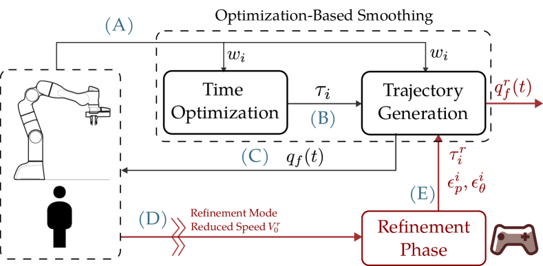
Figure 2: DFL-TORO workflow. Red arrows indicate interactive procedures with the human-robot in the loop.

DFL-TORO workflow (Fig. 2) is detailed as follows:

• The human teacher provides an inherently noisy demonstration $q_{o}(t)$ to a $n$ DoF manipulator via kinesthetic guidance, where the underlying path is extracted and represented as $m$ waypoints, denoted by $w_{i}$ for $\forall i=1,\cdots,m$. The waypoints encode the joint configuration $Q_{w_{i}}\in\mathbb{R}^{n}$, as well as the end-effector’s position $p_{w_{i}}=[x_{w_{i}},y_{w_{i}},z_{w_{i}}]^{T}\in\mathbb{R}^{3}$ and orientation $\theta_{w_{i}}\in\mathbb{S}^{3}$.

• “Time Optimization” module computes the ideal timing $\tau_{i}\in[0,1]$ for $\forall i=1,\cdots,m$ for each waypoint.

• “Trajectory Generation” module solves a comprehensive optimization problem to minimize the jerk. Given that specific task tolerances are not extracted yet, default tolerance values $\epsilon^{d}_{p}\in\mathbb{R}^{3}$ and $\epsilon^{d}_{\theta}\in\mathbb{R}$ are incorporated to generate an initial trajectory. $\epsilon^{d}_{p}$ represents the tolerance in Cartesian position, while $\epsilon^{d}_{\theta}$ signifies the angular difference tolerance. Consequently, the outcome of this hierarchical optimization procedure is a minimum-time, smooth trajectory $q_{f}(t)$.

• “Refinement Phase” allows the teacher to interactively slow down and correct the timing law. The robot replays the trajectory, allowing the human teacher to visually assess the execution speed. The teacher can pinpoint areas where the speed is either unreliable or unsafe and determine which segments require slowing down. Since the current trajectory $q_{f}(t)$ executes very rapidly, it leaves no time for humans to observe the motion and provide feedback. Therefore, the Refinement Phase operates at a reduced speed $V_{0}^{r}\in\mathbb{R}_{+}$, giving humans enough reaction time to make changes.

• Refinement Phase provides revised timings for the trajectory, denoted as $\tau_{i}^{r}\in[0,1]$, as well as the task tolerances $\epsilon_{p}^{i}\in\mathbb{R}^{3}$ and $\epsilon_{\theta}^{i}\in\mathbb{R}$ extracted from human feedback. These updated values are subsequently fed to Trajectory Generation module which leads to a fine-tuned trajectory $q_{f}^{r}(t)$ in accordance with the new timings and tolerances.

The steps of the proposed demonstration framework is provided in Algorithm 1, and elaborated in the following.

III-A Optimization-based Smoothing

We employ B-Splines to represent trajectories in our approach. B-Splines are ideal for robot manipulator trajectory optimization due to their smoothness, local control, and efficient computation [23]. Their piecewise polynomial nature ensures smooth motion paths, making them highly suitable for complex motion planning. A B-spline curve is defined as a linear combination of control points $P_{i^{*}},{i^{*}}=1,\cdots,\bar{n}$ and B-spline basis functions $N_{{i^{*}},k}(s)$. Control points $P_{i^{*}}$ determine the shape of the curve. A B-Spline $\xi(s)$ of $k^{th}$ order with $\bar{n}$ control points $P_{1},P_{2},...,P_{\bar{n}}$ is expressed as:

$$\xi(s)=\sum_{{i^{*}}=1}^{\bar{n}}N_{{i^{*}},k}(s)P_{i^{*}},$$ (1)

where $s\in[0,1]$ is the normalized time. Let $u_{1}\leq u_{2}\leq\ldots\leq u_{\bar{m}}$ be the knots and $\bar{m}=\bar{n}+k$, with

$$N_{{i^{*}},1}(s) =\begin{cases}1&\text{if }u_{i^{*}}\leq s<u_{{i^{*}}+1}\\ 0&\text{otherwise}\end{cases},$$

$$N_{{i^{*}},k}(s) =\frac{s-u_{i^{*}}}{u_{{i^{*}}+k-1}-u_{i^{*}}}N_{{i^{*}},k-1}(s)$$

$$+\frac{u_{{i^{*}+k}}-s}{u_{{i^{*}+k}}-u_{{i^{*}+1}}}N_{{i^{*}+1},k-1}(s).$$

$\xi(s)$ is associated with a duration parameter $T$, which maps the normalized time $s$ into actual time $t$ [23]. $P_{i^{*}}$ and $T$ are the optimization variables. In the following, we describe two modules of optimization-based smoothing.

III-A1 Time Optimization Module

The objective of this optimizer is to find the minimum-time trajectory $q_{t}(t)$ that strictly passes through all the waypoints $Q_{w_{i}}$. At this stage, we ignore constraints related to acceleration and jerk since the noise is still present in the path. Adding such constraints would prevent the optimizer from finding the ideal timings. B-Spline sub-trajectories $\xi_{j}$ for $\forall j=1,\cdots,m-1$ are used to represent the trajectory between every two adjacent waypoints $w_{j}$ and $w_{j+1}$, with control points $P_{{i^{*}},j}$ and durations $T_{j}$. Then, the time optimization problem is formulated as:

$$(P^{*}_{{i^{*}},j},T^{*}_{j}) =\underset{P_{{i^{*}},j},T_{j}}{\mathrm{arg\,min}}\sum_{j=1}^{m-1}T_{j},$$ (2a)

$$q_{j}(t_{j}) =\xi_{j}(\frac{t_{j}}{T_{j}}),$$ (2b)

$$q_{\text{min}} \leq q_{j}(t_{j})\leq q_{\text{max}},$$ (2c)

$$v_{\text{min}} \leq\dot{q}_{j}(t_{j})\leq v_{\text{max}},$$ (2d)

$$\xi_{j}(0) =Q_{w_{j}},$$ (2e)

$$\xi_{j}(1) =Q_{w_{j+1}},$$ (2f)

$$\dot{\xi}_{1}(0) =\dot{\xi}_{m-1}(1)=0,$$ (2g)

for $\forall t_{j}\in[0,T_{j}]$. (2b) relates the normalized and actual trajectories. We set bounds $q_{\text{min}}$, $q_{\text{max}}$, $v_{\text{min}}$ and $v_{\text{max}}\in\mathbb{R}^{n}$ for joint position and velocity as (2c) and (2d), respectively. Note that “$\leq$” represents element-wise inequality of vectors. Continuity constraints (2e) and (2f) are applied at the intersection of these sub-trajectories. (2g) enforces the trajectory to start and rest with zero velocity. The optimization yields an unrealistic trajectory due to the existing noise, with high acceleration and jerk values. (2a) determines the ideal timings $T^{*}_{j}$ to move through all waypoints with highest velocity, which provides normalized time $\tau_{i}$ defined as

$$\tau_{i} =\begin{cases}\frac{\sum_{j=1}^{i-1}T^{*}_{j}}{T^{*}_{m-1}}&i\geq 2\\ 0&i=1\end{cases},$$ (3)

which sets the groundwork for Trajectory Generation module, that addresses the full optimization problem.

III-A2 Trajectory Generation Module

Given $\tau_{i}$, we fit one B-Spline across all the waypoints, denoted as $\xi_{f}$ with control points $P_{i,f}$ and duration variable $T_{f}$. We match the number of control points with the waypoints, i.e., $\bar{n}=m$, giving flexibility to the optimizer to locally adjust the trajectory around each waypoint. The cost function is formulated as:

$$J_{f}=\alpha T_{f}+\beta\int_{0}^{1}||\dddot{\xi}_{f}||^{2}ds+\gamma\sum_{i=1}^{m}||P_{i,f}-Q_{w_{i}}||^{2},$$ (4)

where $\alpha,\beta$ and $\gamma$ are positive weights. The term $\int_{0}^{1}||\dddot{\xi}_{f}||^{2}ds$ attempts to minimize the normalized jerk profile, exploiting the tolerances of waypoints. This strategy is crucial for eliminating noise while respecting the tolerances. The term $\sum_{i=1}^{m}||P_{i,f}-Q_{w_{i}}||^{2}$ ensures that control points align closely with the original joint configurations at the waypoints. Given the robot manipulator’s kinematic redundancy, an end-effector pose can correspond to multiple configurations. This term limits the robot’s configuration null space, prompting the optimizer to remain near the initial configuration. The trajectory generation problem is formulated as follows:

$$(P^{*}_{i,f},T^{*}_{f}) =\underset{P_{i,f},T_{f}}{\mathrm{arg\,min}}\,J_{f},$$ (5a)

$$q_{f}(t) =\xi_{f}(\frac{t}{T_{f}}),$$ (5b)

$$q_{\text{min}} \leq q_{f}(t)\leq q_{\text{max}},$$ (5c)

$$v_{\text{min}} \leq\dot{q}_{f}(t)\leq v_{\text{max}},$$ (5d)

$$a_{\text{min}} \leq\ddot{q}_{f}(t)\leq a_{\text{max}},$$ (5e)

$$J_{\text{min}} \leq\dddot{q}_{f}(t)\leq J_{\text{max}},$$ (5f)

$$\xi_{f}(0) =Q_{w_{1}},$$ (5g)

$$\xi_{f}(1) =Q_{w_{m}},$$ (5h)

$$\dot{\xi}_{f}(0) =\dot{\xi}_{f}(1)=0,$$ (5i)

$$(p_{f}(t),\theta_{f}(t)) =F_{K}(q_{f}(t)),$$ (5j)

$$-\epsilon_{p}^{i}\leq p_{f}( \tau_{i}T_{f})-p_{w_{i}}\leq\epsilon_{p}^{i},$$ (5k)

$$\mathsf{QuatDiff} (\theta_{f}(\tau_{i}T_{f}),\theta_{w_{i}})\in[0,\epsilon_{\theta}^{i}],$$ (5l)

for $\forall t\in[0,T_{f}]$. We have introduced acceleration and jerk bounds $a_{\text{min}}$, $a_{\text{max}}$, $J_{\text{min}}$ and $J_{\text{max}}\in\mathbb{R}^{n}$ in (5e) and (5f), respectively, to ensure the trajectory’s feasibility. Constraints (5g)-(5i) enforce the trajectory to start at $Q_{w_{1}}$ and rest at $Q_{w_{m}}$ with zero velocity. (5j) represents the forward kinematic function $F_{K}$, which is used to assign the tolerance in the end-effector’s Cartesian space with $p_{f}(t)=[x_{f}(t),y_{f}(t),z_{f}(t)]\in\mathbb{R}^{3}$ and $\theta_{f}(t)\in\mathbb{S}^{3}$. The goal is to limit the position and angle deviation of the end-effector at each waypoint $w_{i}$ to $\epsilon_{p}^{i}$ and $\epsilon_{\theta}^{i}$, via (5k) and (5l), respectively, at normalized time $\tau_{i}$. In (5k), “$\leq$” represents element-wise inequality of vectors. $\mathsf{QuatDiff}(.,.)\in[0,\pi]$ is a conventional function to compute the absolute angle difference of two quaternions [24]. Solving (5a) yields $P^{*}_{i,f}$, with which $q_{f}(t)$ is computed using (1) and (5b).

(A): Kinesthetic Guidance

Input: Noisy human demonstration $q_{o}(t)$

Output: Path waypoints $W_{i}=\left(Q_{w_{i}},p_{w_{i}},\theta_{w_{i}}\right)$

(B): Time Optimization

Input: $W_{i}$

Find ideal timings using (2a)-(2g) and (3)

Output: Initial timings $\tau_{i}$

(C): Trajectory Generation

Input: $W_{i}$, $\tau_{i}$, default tolerances $\epsilon_{p}^{d},\epsilon_{\theta}^{d}$

Solve for smooth trajectory using (5a)-(5l)

Output: Trajectory $q_{f}(t)$

(D): Refinement Phase

Input: $q_{f}(t)$, human command $C(t),\eta$

Initialize $v(0)=V_{0}^{r},s_{r}(0)=V_{0}^{r}\cdot t$

while Replaying Trajectory do

       Compute $R(t)$ using (6)

       Compute $s_{r}(t)$ using (7)

       Send $\xi(s_{r}(t))$ to robot for interactive feedback

end while

Compute new timings $\tau_{i}^{r}$ using (8)

for each $w_{i}$ do

       $\epsilon_{p}^{i}\leftarrow\Gamma_{p}(\tau_{i})$ using (9)

       $\epsilon_{\theta}^{i}\leftarrow\Gamma_{\theta}(\tau_{i})$ using (9)

end for

Output: New timings $\tau_{i}^{r}$, new tolerances $\epsilon_{p}^{i},\epsilon_{\theta}^{i}$

(E): Trajectory Fine-Tuning

Input: $W_{i},\tau_{i}^{r},\epsilon_{p}^{i},\epsilon_{\theta}^{i}$

Re-optimize $q_{f}(t)$ via updated timings and tolerances using (5a)-(5l)

Output: Optimal Demonstration $q_{f}^{r}(t)$

Algorithm 1 DFL-TORO Architecture

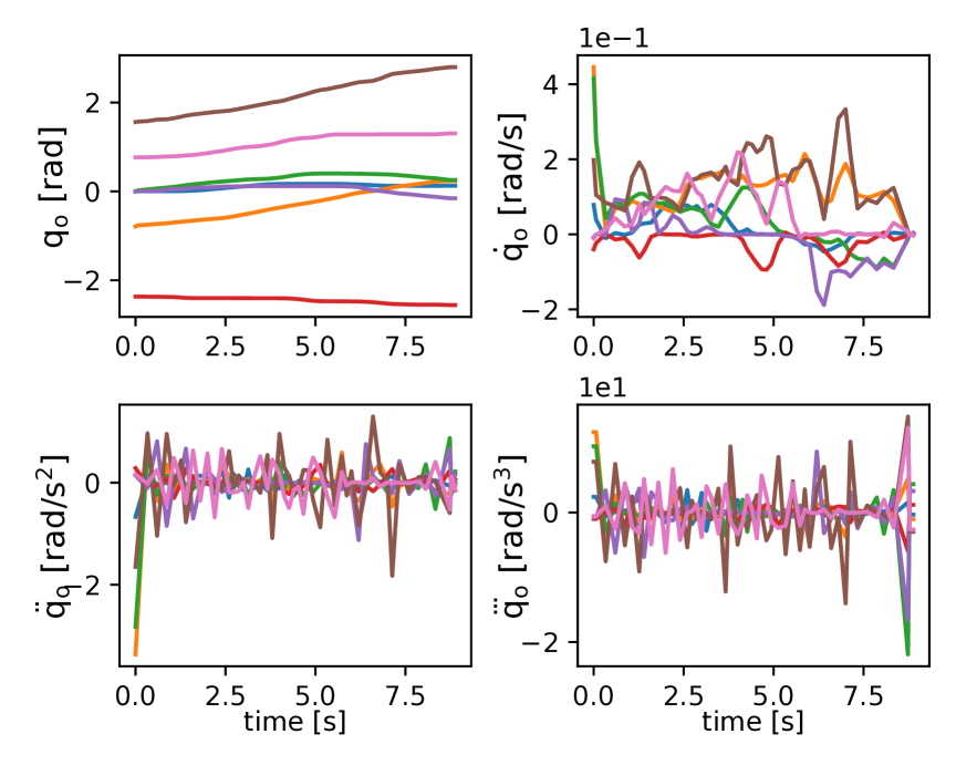
(a) Original Demonstration $q_{o}(t)$

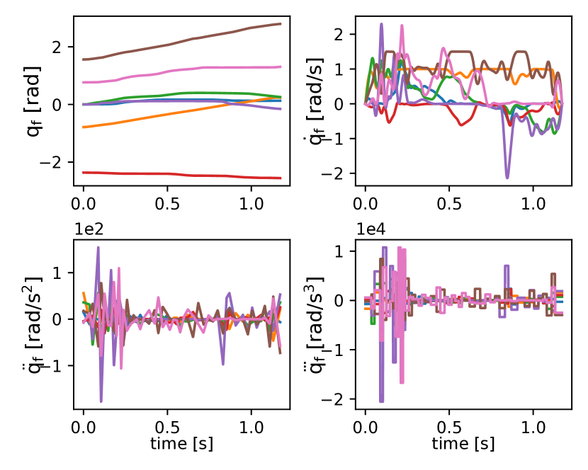
(b) Time Optimization Output $q_{t}(t)$

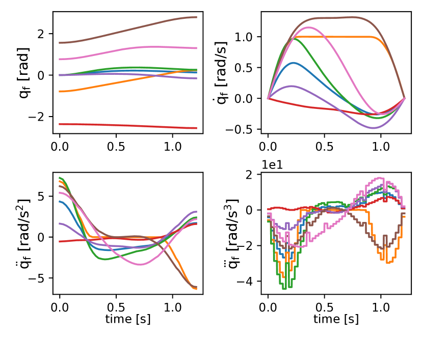
(c) Trajectory Generation Output $q_{f}(t)$

Figure 3: Evolution of RT1 from original to smooth time-optimal joint trajectory. Each color represents a distinct DoF.

III-B Refinement Phase

During Refinement Phase, the teacher can practically slow down the time progression and hence the trajectory velocity. To do so, the trajectory $q_{f}(t)$ with duration $T_{f}$ is replayed with a reduced speed $V_{0}^{r}=\frac{1}{\eta T_{f}}$ for $\eta>1$, letting the human teacher observe and provide interactive feedback in the loop. This is achieved through a teleoperated command, $C(t)\in[-1,0]$, which functions like a brake pedal. It allows the teacher to safely and intuitively interact with the robot in real-time, controlling its velocity during execution. To attenuate noise or abrupt changes in $C(t)$, we pass it as the attractor point of a virtual spring-damper system:

$$\tau\ddot{R}(t)=K(C(t)-R(t))-D\dot{R}(t).$$ (6)

By carefully setting the values of $\tau$, $K$, and $D$, we can configure (6) to be critically damped, as well as adjust its settling time which, in turn, influences the delay in response to human command. The output $R(t)\in[-1,0]$ is used as a deceleration term to adjust the trajectory velocity, as follows.

III-B1 Velocity Adjustment

Since $q_{f}(t)=\xi_{f}(s(t))$ where $s(t)=V_{0}^{r}\cdot t$, by adjusting $s(t)$ we can directly modify the timing law of the trajectory $q_{f}(t)$. Slowing down specific portions of $\xi_{f}(s(t))$ locally can be done by incorporating $R(t)$ as a notion of time deceleration, which leads to a modified mapping $s_{r}(t)$. We compute this new mapping throughout the refinement phase via a straightforward kinematic model:

$$\left\{\begin{matrix}\dot{v}(t)=R(t)\\ \dot{s}_{r}(t)=v(t)\end{matrix}\right.,\quad\begin{matrix}v(t)\in[V_{min}^{r},V^{r}_{0}],\\ s_{r}(t)\in[0,1]\end{matrix}$$ (7)

To prevent the robot from completely stopping, we bound $v(t)$ to a minimum execution speed $V_{min}^{r}\in\mathbb{R}_{+}$. $s_{r}(t)$ and $\tau_{i}$ are used to determine the updated timing $\tau_{i}^{r}$ as

$$\tau_{i}^{r}=\frac{s_{r}^{-1}(\tau_{i})}{s_{r}^{-1}(\tau_{m})},$$ (8)

where $s_{r}^{-1}$ is the inverse of $s_{r}$ obtained via interpolation. It is worth mentioning that refinement at the reduced speed $V_{0}^{r}$ applies the same proportional adjustment on the real speed of execution, as $\tau_{i}^{r}$ are in normalized time.

III-B2 Tolerance Extraction

To extract the tolerances, we posit a direct correlation between the value of $R(t)$ and the desired level of accuracy at a given point on the trajectory. This means, the more intensively the brake pedal is pressed, the greater the criticality of that trajectory portion, necessitating increased precision. This is captured by introducing the functions $\Gamma_{p}(t)$ and $\Gamma_{\theta}(t)$, defined as:

$$\Gamma_{\kappa}(t)=(\epsilon_{\kappa}^{max}-\epsilon_{\kappa}^{min})(1-(-R(t))^{n+\zeta})+\epsilon_{\kappa}^{min},$$ (9)

where $\kappa\in\{p,\theta\}$. In (9), $R(t)=0$ is associated with maximum tolerances $\epsilon_{p}^{max}$ and $\epsilon_{\theta}^{max}$, whereas a $R(t)=-1$ corresponds to the minimum tolerances $\epsilon_{p}^{min}$ and $\epsilon_{\theta}^{min}$. The parameters $\zeta$ and $n$ determine the shape and curve of $\Gamma_{\kappa}$. By computing $\Gamma_{\kappa}(\tau_{i})$ for each waypoint, we extract the requisite tolerances and pass it along with $\tau_{i}^{r}$ for re-optimization.

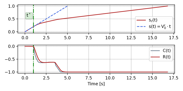
Figure 4: $s(t)$ and $s_{r}(t)$ during the Refinement Phase of RT1. $t^{*}$ marks the moment the teacher starts giving command $C(t)$.

IV Validation Experiments

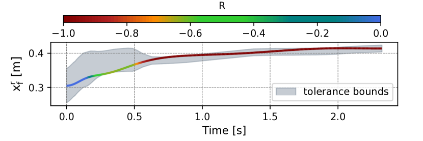
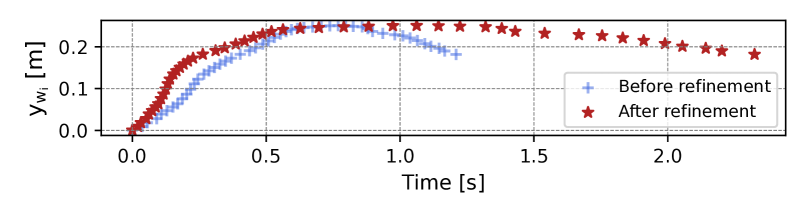
Figure 5: RT1 fine tuning. Upper: $x_{f}^{r}(t)$, with the extracted tolerance ranges via $R(t)$. Lower: waypoints timing law before and after refinement.

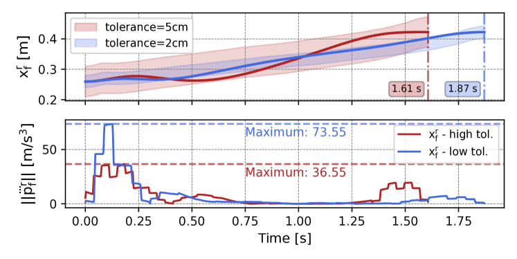
Figure 6: $x_{f}^{r}(t)$ with low and high tolerance ranges, for RT2.

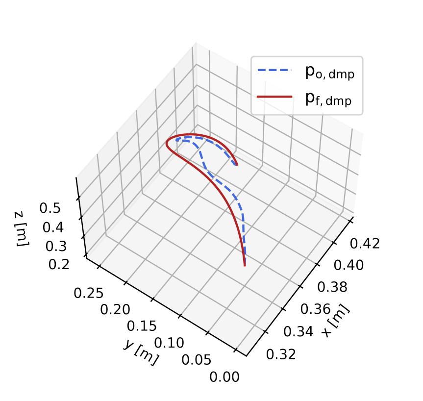
(a) 3D path

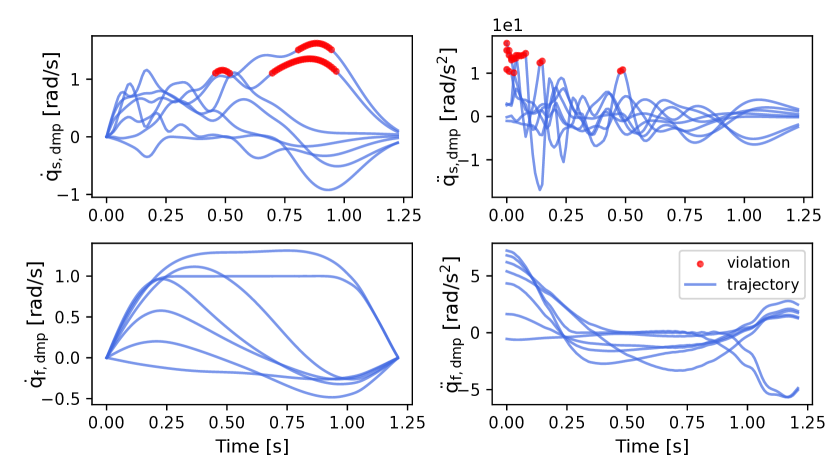
(b) Kinematic violations

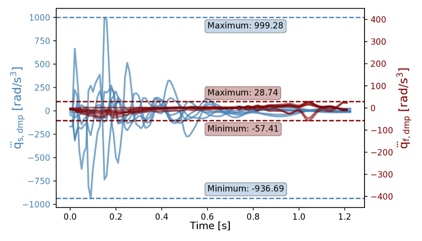
(c) Jerk profiles

Figure 7: Performance comparison of ${\mathrm{DMP}}_{o}$ and ${\mathrm{DMP}}_{f}$ with respect to kinematic feasibility and jerk profiles.

The effectiveness of DFL-TORO is assessed on a 7 DoF FR3 robot in two reaching task scenarios. The performance of Optimization-based Smoothing is analyzed in Sec. IV-B, covering stages (B) and (C) of Algorithm 1. In Sec. IV-C, we examine Refinement Phase (stages (D) and (E)). Using DMP as the learning method, a baseline comparison to the state-of-the-art kinesthetic demonstration is conducted in Sec. IV-D. The choice of DMP is due to the fact that it requires only one demonstration to train. Nevertheless, our proposed method is generic and can be applied to any LfD approach. Note that in order to meaningfully evaluate trajectories with different durations, Maximum Absolute Normalized Jerk (MANJ) in normalized time $s\in[0,1]$ is used. Furthermore, we only illustrate one axis of position trajectory for brevity.

IV-A Experimental Setup

Demonstrations are recorded through kinesthetic guidance using a ROS interface at a frequency of 10 Hz. For teleoperation, we utilize a PS5 wireless controller, receiving continuous brake commands. Waypoints are automatically selected based on an end-effector movement threshold, requiring a shift of at least 1 cm or 0.1 radians for Reaching Task #1 (RT1) and Reaching Task #2 (RT2). The kinematic limits of FR3 are obtained from the robot’s datasheet [25]. B-Splines of order $k=4$ are selected for smoothness up to the velocity level. $u_{1},\cdots,u_{\bar{m}}$ are distributed in a clamped uniform manner [23] to create basis functions in (1). Time Optimization and Trajectory Generation modules are implemented using the Drake toolbox [26]. The weights in (4) are set as $\alpha=1$, $\beta=0.04$, and $\gamma=1$. Finally, default tolerance values are chosen as $\epsilon^{d}_{p}=[2,2,2]$ cm and $\epsilon^{d}_{\theta}=0.1$ radians. In Refinement Phase, we select $\eta=5$, $V_{min}^{r}=0.2V_{0}^{r}$, $\tau=0.1$, $D=20$, and $K=100$. Also, we choose $\epsilon_{p}^{max}=[5,5,5]$ cm, $\epsilon_{p}^{min}=[1,1,1]$ cm, $\epsilon_{\theta}^{max}=0.3$ radians, and $\epsilon_{\theta}^{min}=0.1$ radians. For illustration, $p_{f}^{r}(t)=[x_{f}^{r}(t),y_{f}^{r}(t),z_{f}^{r}(t)]$, representing the Cartesian position trajectory associated with $q_{f}^{r}(t)$, is considered. Besides lowering tolerances in the precise portions, we assign maximum tolerance for $C(t)=0$, providing more freedom for Trajectory Generation to adapt the motion. This is best shown via RT2, where higher tolerances allow the optimizer to find better solutions. We implement DMP in the joint space via [27], to study the effectiveness of DFL-TORO on RT1 in terms of kinematic feasibility and jerk regulation.

IV-B Performance of Optimization-based Smoothing

The original demonstration’s joint trajectory $q_{o}(t)$ is depicted in Fig. 3(a). The original demonstration’s velocity, acceleration, and jerk are differentiated in a non-casual manner [27]. Notably, the demonstration trajectory is slow, while noise reflects itself in the jerk profile. Fig. 3(b) shows the output of the Time Optimization module, stage (B), yielding $q_{t}(t)$ with $\tau_{i}$ extracted via (3). Using $\tau_{i}$ along with $\epsilon^{d}_{p}$ and $\epsilon^{d}_{\theta}$ in stage (C) leads to $q_{f}(t)$, a smooth, noise-free, and time-optimal trajectory shown in Fig. 3(c). $q_{o}(t)$ and $q_{f}(t)$ are compared in Table I considering the metrics of execution time and MANJ. Evidently, DFL-TORO has significantly improved the demonstration quality.

IV-C Demonstration Refinement

Given $C(t)$, the progression of $s(t)$, $s_{r}(t)$ and $R(t)$ (using (6)) are depicted in Fig. 4 (stage (D)). Initially, without any command, $s(t)$ and $s_{r}(t)$ overlap, leaving the timing law unchanged. Upon receiving the command at $t^{*}$, $s_{r}(t)$ progression changes to slow down the motion and thus extend execution time. This revised mapping leads to the derivation of $\tau_{i}^{r}$ using (8). Also, we extract $\epsilon_{p}^{i}$ and $\epsilon_{\theta}^{i}$ via (9). Fig. 5 shows $x_{f}^{r}(t)\in p_{f}^{r}(t)$, the fine-tuned trajectory (stage (E)). The tolerance range is adjusted to be more precise towards the end of reaching, where slow speed was commanded, shown in Fig. 4. Moreover, to showcase the velocity adjustment effect on the trajectory’s timing law, we present the distribution of $y_{w_{i}}$ over the trajectory before and after refinement. Evidently, the waypoints are stretched towards the end of the task. It is also noticeable that while the timing law of the beginning of the trajectory is left unchanged during refinement, the waypoint distribution does not overlap. This is due to the fact that since the tolerance values are increased from $\epsilon_{p}^{d}$ to $\epsilon_{p}^{max}$, as in (9), the optimizer has managed to find a faster trajectory to traverse these waypoints. Fig. 6 shows the effect of increasing tolerance values in RT2, which leads to a 15% reduction in cycle time and a 50% improvement in reducing the maximum jerk.

IV-D Baseline Comparison

For the same start and goal configuration, we train ${\mathrm{DMP}}_{o}$ via $q_{o}(t)$, and ${\mathrm{DMP}}_{f}$ via $q_{f}(t)$, reproducing $q_{o,dmp}(t)$ and $q_{f,dmp}(t)$, respectively. Since $q_{o}(t)$ is slower than $q_{f}(t)$, we leverage the inherent scaling factor in ${\mathrm{DMP}}_{o}$ to produce $q_{s,dmp}(t)$ [10], to have the same duration as $q_{f,dmp}(t)$ for meaningful comparison. Notation-wise, $p_{f,dmp}(t)$ , $p_{o,dmp}(t)$ and $p_{s,dmp}(t)$ represent the associated Cartesian position trajectories. Fig. 7(a) shows the path of $p_{o,dmp}(t)$ and $p_{f,dmp}(t)$. As shown, $p_{o,dmp}(t)$ has produced unnecessary curves at the beginning of the motion, replicating the existing noise. The noise causes $q_{s,dmp}(t)$ to become an infeasible trajectory. The kinematic violations are highlighted in Fig. 7(b), illustrating the infeasibility of $q_{s,dmp}(t)$ while $q_{f,dmp}(t)$ remains feasible for the same execution time. Furthermore, a comparison of the jerk values for $q_{s,dmp}(t)$ and $q_{f,dmp}(t)$ is shown in Fig. 7(c), showcasing that $q_{f,dmp}(t)$ creates significantly lower jerk values. Table I summarizes the time and jerk values for different trajectories associated with RT1. Obviously, the execution time and MANJ metrics are significantly reduced by DFL-TORO. This is further verified by comparing ${\mathrm{DMP}}_{o}$ and ${\mathrm{DMP}}_{f}$. Even though DMP naturally smoothens the original demonstration, $q_{f,dmp}(t)$ still outperforms $q_{o,dmp}(t)$ by a significant margin. Furthermore, although $q_{s,dmp}(t)$ is scaled to the optimal time, it yields an infeasible trajectory with high jerk values, comparing $q_{s,dmp}(t)$ and $q_{f,dmp}(t)$.

TABLE I: Comparison of time and Maximum Absolute Normalized Jerk (MANJ) for RT1.

	Trajectory	Time [$s$]	MANJ [$rad/s^{3}$]
Demonstration	$q_{o}(t)$	$8.88$	$15\,358$
	$q_{f}(t)$	1.2	78.3
DMP	$q_{o,dmp}(t)$	$8.88$	$2305.9$
	$q_{s,dmp}(t)$	$1.2$	$1837$
	$q_{f,dmp}(t)$	1.2	101.5

V Conclusion

In this paper, we presented DFL-TORO, a novel demonstration framework within the LfD process, addressing the poor quality and efficiency of human demonstrations. The framework captures task requirements intuitively with no need for multiple demonstrations, as well as locally adjusting the velocity profile. The obtained trajectory was ensured to be time-optimal, noise-free, and jerk-regulated while satisfying the robot’s kinematic constraints. The effectiveness of DFL-TORO was experimentally evaluated using a FR3 in a reaching task scenario. Future research can explore the richness of information in tolerance values and integrate the task’s semantic nuances. Additionally, by tailoring the learning algorithm, we can improve DMP performance, ensuring optimal output trajectories and more effective motion generalization. Reinforcement Learning is a suitable option for improving DMP generalization in manufacturing contexts.

References

- [1] M. R. Pedersen, L. Nalpantidis, R. S. Andersen, C. Schou, S. Bøgh, V. Krüger, and O. Madsen, “Robot skills for manufacturing: From concept to industrial deployment,” Robot. Comput. Integr. Manuf., vol. 37, pp. 282–291, 2016.
- [2] Y. Cohen, H. Naseraldin, A. Chaudhuri, and F. Pilati, “Assembly systems in industry 4.0 era: a road map to understand assembly 4.0,” Int. J. Adv. Manuf. Technol., vol. 105, pp. 4037–4054, 2019.
- [3] C. Sloth, A. Kramberger, and I. Iturrate, “Towards easy setup of robotic assembly tasks,” Adv. Robot, vol. 34, no. 7-8, pp. 499–513, 2020.
- [4] Z. Liu, Q. Liu, W. Xu, L. Wang, and Z. Zhou, “Robot learning towards smart robotic manufacturing: A review,” Robot. Comput. Integr. Manuf., vol. 77, p. 102360, 2022.
- [5] P. Pastor, M. Kalakrishnan, S. Chitta, E. Theodorou, and S. Schaal, “Skill learning and task outcome prediction for manipulation,” in 2011 IEEE Int. Conf. Robot. Autom. (ICRA), pp. 3828–3834, IEEE, 2011.
- [6] H. Ravichandar, A. S. Polydoros, S. Chernova, and A. Billard, “Recent advances in robot learning from demonstration,” Annu. Rev. Control Robot. Auton. Syst., vol. 3, pp. 297–330, 2020.
- [7] H. Wu, W. Yan, Z. Xu, and X. Zhou, “A framework of improving human demonstration efficiency for goal-directed robot skill learning,” IEEE Trans. Cogn. Develop. Syst., vol. 14, no. 4, pp. 1743–1754, 2021.
- [8] A. Mészáros, G. Franzese, and J. Kober, “Learning to pick at non-zero-velocity from interactive demonstrations,” IEEE Robot. Autom. Lett., vol. 7, no. 3, pp. 6052–6059, 2022.
- [9] M. Simonič, T. Petrič, A. Ude, and B. Nemec, “Analysis of methods for incremental policy refinement by kinesthetic guidance,” J. Intell. Robot. Syst., vol. 102, no. 1, p. 5, 2021.
- [10] A. J. Ijspeert, J. Nakanishi, H. Hoffmann, P. Pastor, and S. Schaal, “Dynamical movement primitives: learning attractor models for motor behaviors,” Neural Comput., vol. 25, no. 2, pp. 328–373, 2013.
- [11] Z. Cao, Z. Wang, and D. Sadigh, “Learning from imperfect demonstrations via adversarial confidence transfer,” in 2022 Int. Conf. Robot. Autom. (ICRA), pp. 441–447, IEEE, 2022.
- [12] A. Kalinowska, A. Prabhakar, K. Fitzsimons, and T. Murphey, “Ergodic imitation: Learning from what to do and what not to do,” in 2021 IEEE Int. Conf. Robot. Autom. (ICRA), pp. 3648–3654, IEEE, 2021.
- [13] B. Nemec, L. Žlajpah, S. Šlajpa, J. Piškur, and A. Ude, “An efficient pbd framework for fast deployment of bi-manual assembly tasks,” in 2018 IEEE-RAS 18th Int. Conf. Humanoid Robots (Humanoids), pp. 166–173, IEEE, 2018.
- [14] S. Calinon, “A tutorial on task-parameterized movement learning and retrieval,” Intell. Serv. Robot., vol. 9, pp. 1–29, 2016.
- [15] Y.-Y. Tsai, B. Xiao, E. Johns, and G.-Z. Yang, “Constrained-space optimization and reinforcement learning for complex tasks,” IEEE Robot. Autom. Lett., vol. 5, no. 2, pp. 683–690, 2020.
- [16] Y. Chen, Q. Feng, and J. Guo, “The playback trajectory optimization algorithm for collaborative robot,” in 2018 IEEE Int. Conf. Robot. Biomimetics (ROBIO), pp. 1671–1676, IEEE, 2018.
- [17] R. A. Shyam, P. Lightbody, G. Das, P. Liu, S. Gomez-Gonzalez, and G. Neumann, “Improving local trajectory optimisation using probabilistic movement primitives,” in 2019 IEEE/RSJ Int. Conf. Intel. Robots Syst. (IROS), pp. 2666–2671, IEEE, 2019.
- [18] D. Müller, C. Veil, M. Seidel, and O. Sawodny, “One-shot kinesthetic programming by demonstration for soft collaborative robots,” Mechatronics, vol. 70, p. 102418, 2020.
- [19] H. Hu, X. Yang, and Y. Lou, “A robot learning from demonstration framework for skillful small parts assembly,” Int. J. Adv. Manuf. Technol., vol. 119, no. 9-10, pp. 6775–6787, 2022.
- [20] L. Roveda, M. Magni, M. Cantoni, D. Piga, and G. Bucca, “Assembly task learning and optimization through human’s demonstration and machine learning,” in 2020 IEEE Int. Conf. Syst. Man Cyber. (SMC), pp. 1852–1859, IEEE, 2020.
- [21] P. M. Fitts, “The information capacity of the human motor system in controlling the amplitude of movement.,” J. Exp. Psychol., vol. 47, no. 6, p. 381, 1954.
- [22] H. Yang, J. Qi, Y. Miao, H. Sun, and J. Li, “A new robot navigation algorithm based on a double-layer ant algorithm and trajectory optimization,” IEEE Trans. Indust. Elect., vol. 66, no. 11, pp. 8557–8566, 2018.
- [23] C. De Boor, “On calculating with b-splines,” J. Approx. Theory, vol. 6, no. 1, pp. 50–62, 1972.
- [24] J. M. McCarthy, Introduction to theoretical kinematics. MIT press, 1990.
- [25] F. Emika, “Robot and interface specifications — franka control interface (fci) documentation,” 2023.
- [26] R. Tedrake and the Drake Development Team, “Drake: Model-based design and verification for robotics,” 2019.
- [27] F. Stulp and G. Raiola, “Dmpbbo: A versatile python/c++ library for function approximation, dynamical movement primitives, and black-box optimization,” J. Open Source Softw., 2019.